Performance Analysis of Matlab Code and PCT Technology Services LSU HPC Training Series, Fall 2017...
45
Information Technology Services LSU HPC Training Series, Fall 2017 p. 1/45 Performance Analysis of Matlab Code and PCT Xiaoxu Guan High Performance Computing, LSU September 27, 2017 1 tic; 2 nsize = 10000; 3 for k = 1:nsize 4 B(k) = sum( A(:,k) ); 5 end 6 toc;
Transcript of Performance Analysis of Matlab Code and PCT Technology Services LSU HPC Training Series, Fall 2017...

Information Technology ServicesLSU HPC Training Series, Fall 2017 p. 1/45
Performance Analysis ofMatlab Code and PCT
Xiaoxu Guan
High Performance Computing, LSU
September 27, 20171 tic;2 nsize = 10000;3 for k = 1:nsize4 B(k) = sum( A(:,k) );5 end6 toc;

Information Technology ServicesLSU HPC Training Series, Fall 2017 p. 2/45
Overview
• Why should we optimize the Matlab code?
• When should we optimize Matlab code?
• What can we do with the optimization of the Matlab
code?
• Profiling and benchmark Matlab applications
• General techniques for performance tuning
• Some Matlab-specific optimization techniques
• Remarks on using Matlab on LSU HPC and LONI
clusters
• Further reading

Information Technology ServicesLSU HPC Training Series, Fall 2017 p. 3/45
Why should we optimize the Matlab code?
• Matlab has broad applications in a variety of disciplines:
engineering, science, applied maths, and economics;
• Matlab makes programming easier compared to others;
• It supports plenty of builtin functions (math functions, matrix
operations, FFT, etc);
• Matlab is both a scripting and programming language;
• Newer version focuses on Just-In-Time (JIT) engine for
compilation;
• Interfacing with other languages: Fortran, C, Perl, Java, etc;
• In some case, Matlab code may suffer more performance
penalties than other languages;
• Optimization means (1) increase FLOPs per second.
(2) make those that are impossible possible;

Information Technology ServicesLSU HPC Training Series, Fall 2017 p. 4/45
When should we optimize Matlab code?
• The first thing is to make your code work to some extent;
• Debug and test your code to produce correct results, even it
runs slowly;
• While the correct results are maintained, if necessary, try to
optimize it and improve the performance;
• Optimization includes (1) adopting a better algorithm, (2) to
implement the algorithm, data and loop structures, array
operations, function calls, etc, (3) how to parallelize it;
• Write the code in an optimized way at the beginning;
• Optimization may or may not be a post-processing
procedure;
• In some cases, we won’t be able to get anywhere if we don’t
do it right: make impossible possible;

Information Technology ServicesLSU HPC Training Series, Fall 2017 p. 5/45
What to do with optimization of Matlab code?
• Most general optimization techniques applied;
• In addition, there are some techniques that are unique to
Matlab code;
• Identify where the bottlenecks are (hot spots);
◦ Data structure;
◦ CPU usage;
◦ Memory and cache efficiency;
◦ Input/Output (I/O);
◦ Builtin functions;
• Though we cannot directly control the performance ofbuiltin functions, we have different options to choose abetter one;
• Let Matlab use JIT engine as much as possible;

Information Technology ServicesLSU HPC Training Series, Fall 2017 p. 6/45
Profiling and benchmark Matlab applications
• Overall wall-clock time can be obtained from the job log, but
this might not be what we want;
• Matlab 5.2 (R10) or higher versions provide a builtin profiler:
$ matlab
$ matlab -nosplash % don’t display logo$ matlab -nodesktop -nosplash % turn desktop off$ matlab -nodesktop -nosplash -nojvm % java engine off
• On a matlab terminal, let’s run
>> profile on # turn the profiler on>> nsize = 10000;
>> myfunction(nsize); # call a function>> profile off # turn the profiler off>> profile viewer # A GUI report

Information Technology ServicesLSU HPC Training Series, Fall 2017 p. 7/45
Profiling and benchmark Matlab applications
• The profiler sorts time elapsed for all functions, and reports
the number of calls, the time-consuming lines and block;
• Time is reported in both percentage and absolute value;
• It is not required to modify your code;
• A simple and efficient way to use the builtin functions:
tic and toc (elapsed time in seconds);
. . . . . . ; % initialize the arraytic; % start timer at 0nsize = . . . . . .;for k = 1:nsize
vectora(k,1) = matrix_b(k,5) + matrix_c(k,3);
end
toc; % stop timerElapsed time is 18.309452 seconds.

Information Technology ServicesLSU HPC Training Series, Fall 2017 p. 8/45
Profiling and benchmark Matlab applications
• tic/toc can be used to measure elapsed time in a morecomplicated way;
• Let’s consider two nested loops: how to measure the outer
and inner loops separately:
nsize = 3235;
A=rand(nsize); b=rand(nsize,1); c=zeros(nsize,1);
tic;
for i = 1:nsize % outer loopA(i,i) = A(i,i) - sum(sum(A));
for j = 1:nsize % inner loopc(i,1) = c(i,1) + A(i,j)*b(j,1);
end
end
toc; tictoc_loops_v0.m

Information Technology ServicesLSU HPC Training Series, Fall 2017 p. 9/45
Profiling and benchmark Matlab applications
• tic/toc can be used to measure elapsed time in a morecomplicated way:
timer_inner = 0; timer_outer = 0;
for i = 1:nsize % outer looptic;
A(i,i) = A(i,i) - sum(sum(A));
timer_outer = timer_outer + toc;
tic; tictoc_loops_v1.mfor j = 1:nsize % inner loop
c(i,1) = c(i,1) + A(i,j)*b(j,1);
end
timer_inner = timer_inner + toc;
end
fprintf(’Inner loop % f seconds\n’, timer_inner);
fprintf(’Outer loop % f seconds\n’, timer_outer);

Information Technology ServicesLSU HPC Training Series, Fall 2017 p. 10/45
General techniques for performance tuning
• We discuss some general aspects of optimization techniques
that are applied to Matlab and other codes;
• It is mostly about loop-level optimization:
◦ Hoist index-invariant code segments outsideof loops.
◦ Avoid unnecessary computation.
◦ Nested loops and change loop orders.
◦ Optimize the data structure if necessary.
◦ Loop merging/split (unrolling).
◦ Optimize branches in loops.
◦ Use inline functions.
◦ Spatial and temporal data locality.

Information Technology ServicesLSU HPC Training Series, Fall 2017 p. 11/45
General techniques for performance tuning
• Hoist index-invariant code segments outside of loops;
• Consider the same code tictoc_loops_v1.m and then _v2.m:
timer_inner = 0; timer_outer = 0;
for i = 1:nsize % outer looptic;
A(i,i) = A(i,i) - sum(sum(A));
timer_outer = timer_outer + toc;
tic; tictoc_loops_v1.mfor j = 1:nsize % inner loop
c(i,1) = c(i,1) + A(i,j)*b(j,1);
end
timer_inner = timer_inner + toc;
end
fprintf(’Inner loop % f seconds\n’, timer_inner);
fprintf(’Outer loop % f seconds\n’, timer_outer);

Information Technology ServicesLSU HPC Training Series, Fall 2017 p. 12/45
General techniques for performance tuning
• Hoist index-invariant code segments outside of loops;
• Consider the same code tictoc_loops_v1.m and then _v2.m:
timer_inner = 0; timer_outer = 0;
for i = 1:nsize % outer looptic;
A(i,i) = A(i,i) - sum(sum(A)) ; % out of the looptimer_outer = timer_outer + toc;
tic; tictoc_loops_v2.mfor j = 1:nsize % inner loop
c(i,1) = c(i,1) + A(i,j)*b(j,1);
end
timer_inner = timer_inner + toc;
end
fprintf(’Inner loop % f seconds\n’, timer_inner);
fprintf(’Outer loop % f seconds\n’, timer_outer);

Information Technology ServicesLSU HPC Training Series, Fall 2017 p. 13/45
General techniques for performance tuning
• Hoist index-invariant code segments outside of loops;
• Consider the same code tictoc_loops_v1.m and then _v2.m:
• tictoc_loops_v1.m:
>> The time elapsed for inner loop is 0.926248 s.
>> The time elapsed for outer loop is 5.810867 s.
>> The total time is 6.769521 s.
• tictoc_loops_v2.m:
>> The time elapsed for inner loop is 0.488543 s.
>> The time elapsed for outer loop is 0.002263 s.
>> The total time is 0.521508 s.
• The overall speedup is 13×: we only touched the outer loop;
• Why does it affect the inner loop in a positive way?
• How can we optimize the inner loop?

Information Technology ServicesLSU HPC Training Series, Fall 2017 p. 14/45
Avoid unnecessary computation
• This might be attributed to reengineering your algorithms:
• Let’s consider a vector operation: vout = exp (iz1)exp (iz2)
nsize = 8e+6;
. . . . . .;cvector_inp_1 = complex(vector_zero,vector_inp_1);
cvector_inp_2 = complex(vector_zero,vector_inp_2);
for i = 1:nsize
cvector_out_1(i,1) = exp( cvector_inp_1(i,1) ) ;
end
for i = 1:nsize
cvector_out_2(i,1) = exp( cvector_inp_2(i,1) ) ;
end avoid_unness_v0.mcvectort_out_3 = cvector_out_1 .* cvector_out_2 ;
>> Elapsed time is 2.303156 s.
Information Technology ServicesLSU HPC Training Series, Fall 2017 p. 15/45
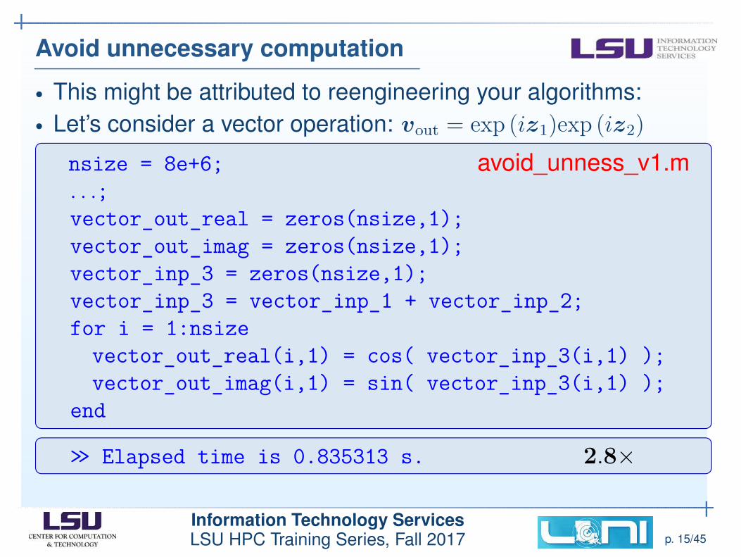
Avoid unnecessary computation
• This might be attributed to reengineering your algorithms:
• Let’s consider a vector operation: vout = exp (iz1)exp (iz2)
nsize = 8e+6; avoid_unness_v1.m. . .;vector_out_real = zeros(nsize,1);
vector_out_imag = zeros(nsize,1);
vector_inp_3 = zeros(nsize,1);
vector_inp_3 = vector_inp_1 + vector_inp_2;
for i = 1:nsize
vector_out_real(i,1) = cos( vector_inp_3(i,1) );
vector_out_imag(i,1) = sin( vector_inp_3(i,1) );
end
>> Elapsed time is 0.835313 s. 2.8×

Information Technology ServicesLSU HPC Training Series, Fall 2017 p. 16/45
Nested loops and change loop orders
• Consider a very simple case: sum over all matrix elements:
a = rand(4000,6000); loop_order_v0.mn = size(a,1);
m = size(a,2);
tic;
total = 0.0;
for inrow = 1:n
for incol = 1:m
total = total + a(inrow,incol); % row-wise sumend
end
>> Elapsed time is 0.700789 s.

Information Technology ServicesLSU HPC Training Series, Fall 2017 p. 17/45
Nested loops and change loop orders
• Consider a very simple case: sum over all matrix elements:
a = rand(4000,6000); loop_order_v1.mn = size(a,1);
m = size(a,2);
tic;
total = 0.0;
for incol = 1:m
for inrow = 1:n % two loops were swappedtotal = total + a(inrow,incol); % column-wise sum
end
end
>> Elapsed time is 0.317501 s. 2.2×
• In matlab, multi-dimensional arrays are stored in column
wise (same as Fortran); What happens to sum(sum(a))?

Information Technology ServicesLSU HPC Training Series, Fall 2017 p. 18/45
Nested loops and change loop orders
• Let’s consider the problem of string vibration with the fixed
ends: ∂2u/∂t2 = c2 ∂2u/∂x2, x ∈ [0, a] and t ∈ [0, T ];
• Initial conditions: u(x, 0) = sin(πx), ∂u(x, 0)/∂t = 0;
• Boundary conditions: u(0, t) = u(a, t) = 0.
• Finite differences in both spatial and temporal coordinates;
• xi = i∆x and tk = k∆t lead to u(xi, tk) = uik;
∂2u(xi, tk)
∂x2≃
1
∆x2[ui+1,k − 2ui,k + ui−1,k], (1)
∂2u(xi, tk)
∂t2≃
1
∆t2[ui,k+1 − 2ui,k + ui,k−1], (2)
ui,k+1 = fui+1,k + 2(1 − f)ui,k + fui−1,k − ui,k−1, (3)
and f = (c∆t/∆x)2.

Information Technology ServicesLSU HPC Training Series, Fall 2017 p. 19/45
Nested loops and change loop orders
• Let’s consider the problem of string vibration with the fixed
ends: ∂2u/∂t2 = c2 ∂2u/∂x2, x ∈ [0, a] and t ∈ [0, T ];
• Initial conditions: u(x, 0) = sin(πx), ∂u(x, 0)/∂t = 0;
• Boundary conditions: u(0, t) = u(a, t) = 0.
• Finite differences in both spatial and temporal coordinates;
• xi = i∆x and tk = k∆t lead to u(xi, tk) = uik;
x
t
u(xi, tk)
x
t
u(xi, tk)
u(xi+1, tk−1)
u(xi, tk−1)
u(xi, tk−2)
u(xi−1, tk−1)

Information Technology ServicesLSU HPC Training Series, Fall 2017 p. 20/45
Nested loops and change loop orders
for jt = 1:Ntime; string_vib_v0.mu(jt,1) = 0.0; u(jt,Nx) = 0.0;
end
for ix = 2:Nx-1
u(1,ix) = sin(pi*x_step);
u(2,ix) = 0.5*const*( u(1,ix+1) + u(1,ix-1) ) . . .+ (1.0-const)*u(1,ix);
end
for jt = 2:Ntime-1
for ix = 2:Nx-1
u(jt+1,ix) = 2.0*(1.0-const)*u(jt,ix) . . .+ const*(u(jt,ix+1) + u(jt,ix-1)) - u(jt-1,ix);
end
end How can we optimize it?
>> Elapsed time is 19.222726 s.

Information Technology ServicesLSU HPC Training Series, Fall 2017 p. 21/45
Nested loops and change loop orders
for jt = 1:Ntime; string_vib_v1.mu(1,jt) = 0.0; u(Nx,jt) = 0.0;
end
for ix = 2:Nx-1
u(ix,1) = sin(pi*x_step);
u(ix,2) = 0.5*const*( u(ix+1,1) + u(ix-1,1) ) . . .+ (1.0-const)*u(ix,1);
end
for jt = 2:Ntime-1
for ix = 2:Nx-1
u(ix,jt+1) = 2.0*(1.0-const)*u(ix,jt) . . .+ const*(u(ix+1,jt) + u(ix-1,jt)) - u(ix,jt-1);
end
end
>> Elapsed time is 0.291292 s. 66×

Information Technology ServicesLSU HPC Training Series, Fall 2017 p. 22/45
Optimize branches in loops
• Loop merging/split (unrolling). Optimize branches in loops;
• Consider a summation: π = 4(1 − 1
3+ 1
5− 1
7+ 1
9−. . . ).
n = 500000; pi_v0.mtotal = 0.0; k= 0;
for id =1:2:n
k = k + 1;
if mod(k,2)==0 tmp = -1.0/double(id);
else tmp = 1.0/double(id);
end
total = total + tmp;
end
total = 4.0 * total;
fprintf(’%15.12f’, total);
>> Elapsed time is 0.043757 s.

Information Technology ServicesLSU HPC Training Series, Fall 2017 p. 23/45
Optimize branches in loops
• Loop merging/split (unrolling). Optimize branches in loops;
• Consider a summation: π = 4(1 − 1
3+ 1
5− 1
7+ 1
9−. . . ).
n = 500000; pi_v1.mtotal = 0.0;
for id =1:4:n
tmp = 1.0/double(id);
total = total + tmp;
end
for id =3:4:n
tmp = -1.0/double(id);
total = total + tmp;
end
total = 4.0 * total;
fprintf(’%15.12f’, total); loop split
>> Elapsed time is 0.023158 s. 1.9×

Information Technology ServicesLSU HPC Training Series, Fall 2017 p. 24/45
Optimize branches in loops
• Loop merging/split (unrolling). Optimize branches in loops;
• Consider a summation: π = 4(1 − 1
3+ 1
5− 1
7+ 1
9−. . . ).
n = 500000; pi_v2.mtotal = 0.0;
fac = 1.0;
for id =1:2:n
tmp = fac/double(id);
total = total + tmp;
fac = -fac;
end
total = 4.0 * total;
fprintf(’%15.12f’, total);
>> Elapsed time is 0.020947 s. 2.0×
• In the last two versions, the branches were removed from the
loops.

Information Technology ServicesLSU HPC Training Series, Fall 2017 p. 25/45
Use inline functions
• Consider the computation of distances between any two
points a(3, ncol) and b(3, ncol) in 3D space:
ncol = 2000; norm_v0.ma = rand(3,ncol);
b = rand(3,ncol);
tic;
for i = 1:ncol
for j = 1:ncol
c(i,j) = norm( a(:,j)-b(:,i) );
end
end
toc;
>> Elapsed time is 15.803001 s.

Information Technology ServicesLSU HPC Training Series, Fall 2017 p. 26/45
Use inline functions
• Consider the computation of distances between any two
points a(3, ncol) and b(3, ncol) in 3D space:
ncol = 2000; norm_v1.ma = rand(3,ncol);
b = rand(3,ncol);
tic;
c = zeros(ncol,ncol); % allocate c array firstfor i = 1:ncol
for j = 1:ncol
c(i,j) = norm( a(:,j)-b(:,i) );
end
end
toc;
>> Elapsed time is 13.185580 s. 1.2×

Information Technology ServicesLSU HPC Training Series, Fall 2017 p. 27/45
Use inline functions
• Consider the computation of distances between any two
points a(3, ncol) and b(3, ncol) in 3D space:
ncol = 2000; norm_v2.ma = rand(3,ncol);
b = rand(3,ncol);
tic;
c = zeros(ncol,ncol); % allocate c array firstfor j = 1:ncol
for i = 1:ncol
c(i,j) = norm( a(:,j)-b(:,i) );
end
end
toc;
>> Elapsed time is 13.153847 s. 1.2×

Information Technology ServicesLSU HPC Training Series, Fall 2017 p. 28/45
Use inline functions
• Consider the computation of distances between any two
points a(3, ncol) and b(3, ncol) in 3D space:
tic; norm_v3.mc = zeros(ncol,ncol); % allocate c array firstfor j = 1:ncol
for i = 1:ncol
x = a(1,j) - b(1,i);
y = a(2,j) - b(2,i);
z = a(3,j) - b(3,i);
c(i,j) = sqrt(x*x + y*y + z*z); % replace normend
end
toc;
>> Elapsed time is 0.472565 s. 33×

Information Technology ServicesLSU HPC Training Series, Fall 2017 p. 29/45
Exercise: solving a set of linear equations
• Let’s consider using the iterative Gauss-Seidel method to
solve a linear system Ax =b (assume that aii 6= 0,
i = 1, 2,. . . ,n);
x(k+1)i =
1
aii
(
bi −∑
j<i
aijx(k+1)j −
∑
j>i
aijx(k)j
)
. (4)

Information Technology ServicesLSU HPC Training Series, Fall 2017 p. 30/45
Exercise: solving a set of linear equations
• Let’s consider using iterative Gauss-Seidel method to solve
a linear system Ax =b (assume that aii 6= 0, i = 1, 2,. . . ,n);
function x = GaussSeidel(A,b,es,maxit)
. . . . . .while (1) GaussSeidel_v0.mxold = x; adapted from Chapra’s Appliced Numerical
for i = 1:n; Methods with MATLAB (2nd ed. p.269)x(i) = d(i) - C(i,:)*x;
if x(i) ∼= 0;
ea(i) = abs((x(i) -xold(i))/x(i)) * 100;
end
end
iter = iter + 1; How can we optimize it?if max(ea) <= es | iter >= maxit, break, end
end

Information Technology ServicesLSU HPC Training Series, Fall 2017 p. 31/45
Exercise: solving a set of linear equations
• Let’s consider using iterative Gauss-Seidel method to solve
a linear system Ax =b (assume that aii 6= 0, i = 1, 2,. . . ,n);
nsize = 6000;
A = zeros(nsize); b = zeros(nsize,1);
es = 0.00001; maxit = 100; driver_GaussSeidel.mfor i = 1:nsize
b(i) = 3.0 - 2.0*sin(double(i)*15.0);
for j = 1:nsize
A(j,i) = cos(double(i-j)*123.0);
end
end
tic;
xsolution = GaussSeidel_v0(A,b,es,maxit);
toc;
>> Elapsed time is 18.823522 s (. . . _v0.m).

Information Technology ServicesLSU HPC Training Series, Fall 2017 p. 32/45
Optimization techniques specific to Matlab
• In addition to understanding general tuning techniques, there
are techniques unique to Matlab programming;
• There are always multiple ways to solve the same problem;
◦ Fast Fourier transform (FFT).
◦ Convert numbers to strings.
◦ Dynamic allocation of arrays.
◦ Construct a sparse matrix.
◦ . . .

Information Technology ServicesLSU HPC Training Series, Fall 2017 p. 33/45
FFT
• Let’s consider the FFT of a series signal:
tic; fft_v0.mnsize = 3e6; nsizet = nsize + 202;
a = rand(1,nsize);
b = fft(a,nsizet);
toc;
>> Elapsed time is 0.650933 s.
tic; fft_v1.mnsize = 3e6;
n = nextpow2(nsize); nsizet = 2ˆn;
a = rand(1,nsize);
b = fft(a,nsizet);
toc;
>> Elapsed time is 0.293406 s. 2.2×

Information Technology ServicesLSU HPC Training Series, Fall 2017 p. 34/45
Preallocation of arrays
• Matlab supports dynamical allocation of arrays;
• It is both good and bad in terms of easy coding and
performance:
My_data=importdata(’input.dat’); array_alloc_v0.mtic;
Sortx=zeros(1,1);
k=0; s=1;
while k<=My_data(1,1)
Sortx(s,1)=My_data(s,4);
s=s+1;
k=My_data(s,1);
end
toc;
>> Elapsed time is 0.056778 s.

Information Technology ServicesLSU HPC Training Series, Fall 2017 p. 35/45
Preallocation of arrays
• It is always a good idea to preallocate arrays:
tic; array_alloc_v1.mk=0; s=1;
while k<=My_data(1,1)
s=s+1; k=My_data(s,1);
end
Sortx=zeros(s-1,1);
k=0; s=1;
while k<=My_data(1,1)
Sortx(s,1)=My_data(s,4);
s=s+1;
k=My_data(s,1);
end
toc;
>> Elapsed time is 0.027005 s. 2.1×

Information Technology ServicesLSU HPC Training Series, Fall 2017 p. 36/45
Convert numbers to strings
• Matlab provides a builtin function num2str:
tic; num2str_v0.mi = 12345.6;
A = num2str(sin(i+i),’%f’);
toc;
>> Elapsed time is 0.019238 s.
tic; num2str_v1.mi = 12345.6;
A = sprintf(’%f’,sin(i+i));
toc;
>> Elapsed time is 0.005372 s. 3.6×
• In this case, sprintf is much better than num2str;

Information Technology ServicesLSU HPC Training Series, Fall 2017 p. 37/45
What we haven’t covered
• There are other Matlab techniques that are not covered here:
◦ Matlab vectorization.
◦ File I/O.
◦ Matlab indexing techniques.
◦ Object oriented programming in Matlab.
◦ Binary MEX code.
◦ Matlab programming on GPUs.
◦ Graphics.
◦ . . .

Information Technology ServicesLSU HPC Training Series, Fall 2017 p. 38/45
MATLAB Parallel Computing Toolbox(PCT)
collin
Text Box

Information Technology ServicesLSU HPC Training Series, Fall 2017 p. 39/45
Parallel computing
• Why do we need parallel computing?
• Solves large problems and save wall-clock time.
◦ Splits large problems into smaller ones anddistribute data across multiple cores and multiplenodes (strong scaling).
◦ Uses the same number of cores or nodes, butincreases the size of problem (weak scaling).
◦ Communication overhead.
◦ Acceleration Matlab apps on Nvidia GPU cards;
• Matlab supports the PCT (on a single node) and Matlab
distributed computing server (MDCS on multiple nodes);
• Matlab supports implicit and explicit multi-processing
(since R2011a);

Information Technology ServicesLSU HPC Training Series, Fall 2017 p. 40/45
Parallel computing
• Note that Matlab has achieved explicit parallelism through a
very different mechanism;
• Matlab supports MDCS on multiple nodes and servers;
• Third-party attempts: PMatlab (MatlabMPI from MIT) to
address the issue on multiple nodes;
• However, LSU HPC only supports PCT (on Xeon and GPU);
• The PCT is available in R2017a and R2015b on Mike-II,
SuperMIC, and Philip;

Information Technology ServicesLSU HPC Training Series, Fall 2017 p. 41/45
PCT: parfor
• Reserve a pool of workers: parpool(poolsize)
• Delete the current pool: delete(gcp)
• Loop-level parallelism: parfor
parpool(16); parfor_loop.mtic; % . . . skip the array initialization.
nsize = 10000000;
parfor k = 1:nsize
a(k) = k - cos(k);
b(k) = k + sin(k);
end
toc;
delete(gcp)
Elapsed time (for) is 2.8075 s.
Elapsed time (parfor, 2 workers) is 1.8576 s.
Elapsed time (parfor, 16 workers) is 0.8224 s. 3.4×

Information Technology ServicesLSU HPC Training Series, Fall 2017 p. 42/45
PCT: parfor
• parfor cannot parallelize all kinds of loops;
• Loop iterations need to independent;
• Don’t try access the nonindexed variables outside parfor;
parpool(2); parfor_loop_vars.mnsize = 20;
a = zeros(1,nsize);
ktmp = 0;
parfor k = 1:nsize
ktmp = k+k+k;
a(k) = ktmp;
end
a
ktmp
delete(gcp)
The array a is good, but ktmp (=0) is not;

Information Technology ServicesLSU HPC Training Series, Fall 2017 p. 43/45
Performance comparison
MatlabMPI
MPI
Message size as a fraction to total memory
Fractionofpeakbandwidth
10010−210−410−610−810−10
100
10−1
10−2
10−3
10−4
10−5
10−6
10−7
Bandwidth
Reproduced fromJ. Kepner,Parallel MATLABfor Multicore andMultinodeComputers(SIAM, 2009)
• Matlab program.: relatively quick anf easy;
MPI program.: hard and longer development cycle;
• Matlab program.: slow perf.; MPI program: best perf.;

Information Technology ServicesLSU HPC Training Series, Fall 2017 p. 44/45
Remarks on LSU HPC and LONI clusters
• On all LSU HPC clusters we do support PCT (but not MDCS);
• We can only run Matlab code on a single node;
• You can run Matlab jobs on multiple cores but without
multi-threading programming. Choose queue properly;
• However, it is possible that Matlab automatically spawns
several threads;
• If you use single queue on SuperMIC, Mike-II, or QB-2, and
if you don’t use PCT, please always add -singleCompThread
in your matlab command line;
• For LONI’s non-LSU and non-ULL users on QB-2, you have
to provide your own license file;
• A lot of performance improvement is potential from r2013 to
r2017;
• Matlab on LSU HPC website;

Information Technology ServicesLSU HPC Training Series, Fall 2017 p. 45/45
Further reading
• Matlab bloggers: http://blogs.mathworks.com
• Accelerating MATLAB Performance
(Y. Altman, CRC Press, 2015)
• Matlab Central (File Exchange)