Wireless Pers CommunDOI 10.1007/s11277-013-1291-9

Performance Analysis of Cooperative Multi-hop StripNetworks

Syed Ali Hassan

© Springer Science+Business Media New York 2013

Abstract A two-dimensional strip-shaped network is analyzed where groups of nodes per-form cooperative transmission and propagate the message in a multi-hop manner along thelength of the network. The transmission from one group of nodes to the next is modeled as adiscrete-time Markov chain and the probability transition matrix of the chain is derived. Byinvoking the theory of Perron–Frobenius, the eigen-decomposition of the matrix providesinsightful information about the coverage of the network and the probability of making finitesuccessful hops. It has been shown that a specific signal-to-noise ratio margin is required forobtaining a desired hop distance for different network topologies and packet delivery ratioconstraints.

Keywords Cooperative communications · Strip networks · Markov chains

1 Introduction

A cooperative transmission (CT) network can often provide reliable data transmission wheretwo or more spatially separated radios combine their signals to form a virtual antenna sys-tem, thereby providing array and diversity gain, range extension, and power efficiency withincreased system capacity [1]. If the source and the destination are far apart, multi-hop mecha-nism can be used with CT employed at each hop. Whereas a single-input single-output (SISO)multi-hop transmission may not provide large coverage of the network owing to the weakSISO links, which are subject to thermal noise and fading, a CT multi-hop network provides

The author gratefully acknowledge the National ICT R&D Fund for sponsoring this research work.

S. A. Hassan (B)School of Electrical Engineering and Computer Science,National University of Sciences and Technology,Islamabad 44000, Pakistane-mail: ali.hassan@seecs.edu.pk

123

S. A. Hassan

reliable data communication between a source and a destination with reduced latency. Theseproperties of CT multi-hop transmission make it a suitable candidate for a wireless networkwhere many nodes are distributed in an area, e.g., an ad hoc or sensor network.

Opportunistic large array (OLA) is a kind of CT network where the message signal hopsfrom a layer of nodes to another [2]. In an OLA transmission, all radios that decode amessage, relay the message together, very shortly after reception, without coordination withother relays. This process continues until the message signal reaches the destination nodeor broadcasted over the entire network. No cluster head is required and the nodes transmitautonomously in response to energy received from the previous level nodes. The well knownadvantages of an OLA network are range extension [3], simple and inexpensive routing [4],MAC-free broadcasting, and energy-efficiency [5].

A considerable literature on OLA assumes a continuum of nodes in the network, whichimplies that the node density in an area goes to infinity while keeping the total transmitpower constant per unit area [6]. This network is generally known as dense network wherethe number of network nodes goes to infinity whereas the size of the network is fixed. In[6], the authors showed that the performance of the network is dependent on the multi-hop diversity and the message can be broadcasted over the entire network. Most resultsare supported by Monte Carlo simulation because of the analytical intractability. In [7],the authors studied an energy-efficient dense OLA network in which all the nodes of onelevel do not transmit; rather a subset of nodes transmit to save energy. They showed thatthis participation could be achieved by using a signal-to-noise ratio (SNR)-based threshold,however, they derived conditions guaranteeing an infinite broadcast. MAC layer and routingprotocols were studied in [4] where the concept of opportunistic routing was introduced.Spatial reuse for dense continuum network for multiple packet transmission from the samesource has been considered in [8].

In [9], the authors analyzed a variant of OLA network for finite node density, whichis known as an extended network. In this type of network, the number of nodes is finiteand size of the network grows for some fixed node density. The authors have shown thateither in one-dimension (1D) or two-dimensions (2D), an infinite broadcast is not possibleand the performance of the network strongly depends on the path loss exponent. The results,however, could not identified the actual coverage of a finite density extended network. In [10],the authors first introduced the quasi-stationary Markov chain approach for analysis of a linenetwork of equally spaced decode-and-forward nodes, which form consecutive OLAs. Theupper bounds on the coverage of the network were derived given a transmit power constraintand a given required quality of service. However, the approach is only limited to finite densitylinear extended networks. Similarly, the authors in [11] studied a linear network, where thegroups of nodes are co-located and provide better coverage areas specially in the cases wherelarger values of path loss exponents are present. Other approaches considering variants ofline networks are discussed in [12–14].

In this paper, we complement the findings of [9] that there is a zero probability of asuccessful broadcast over an entire 2D network, however, we quantify the coverage andperformance of a strip-shaped extended network. We extend the approach in [10] to a morepractical 2D network, where the nodes are aligned on a 2D regular grid. The motivationbehind this study is two folds: (a) 2D grid network can be a prelude to more complex random2D network and can provide insight into the coverage of such systems for a given density,(b) to provide a mechanism on how the 1D linear model can be simply extended for thestudy of 2D networks. The channel model includes path loss with an arbitrary exponent, andindependent Rayleigh fading. The transmission that hop from one layer of nodes to other aremodeled as discrete-time Markov chain and by applying the quasi-stationary Markov chain

123

Cooperative Multi-hop Strip Networks

analysis, we show that there is no condition guaranteeing infinite propagation of OLAs ina two-dimensional network with finite density. There is only a probability of successfullydelivering a packet over a given distance. We quantify the value of signal-to-noise ratio (SNR)margin that guarantees a particular coverage area with a certain quality of service.

The proposed mathematical modeling and the results of this study can provide sufficientinformation to a network deployer to design various network parameters given a length of thenetwork. The model can be utilized to form a uni-cast cooperative route through a network.Many other application include structural health monitoring, smart meters connectivity, faultrecognition in transmission lines, and indoor surveillance and security. The analysis of thisnetwork could also be used in another emerging area of using cooperation in emergencysituations, where the self-organizing nodes route the information from an emergency nodeto a desired destination [15].

The rest of the paper is organized as follows. In the next section, we describe the systemmodel and network parameters. Section 3 proposes a model of the 2D cooperative network viadiscrete-time Markov chains (DTMC) and obtains a quasi-stationary distribution of this chain.The results and system performance are discussed in Sect. 4 and the paper then concludes inSect. 5.

2 System Model

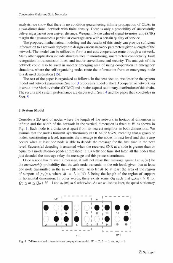
Consider a 2D grid of nodes where the length of the network in horizontal dimension isinfinite and the width of the network in the vertical dimension is fixed at W as shown inFig. 1. Each node is a distance d apart from its nearest neighbor in both dimensions. Weassume that the nodes transmit synchronously in OLAs or levels, meaning that a group ofnodes, constituting a level, transmits the message to the nodes in next level and that a hopoccurs when at least one node is able to decode the message for the first time in the nextlevel. Successful decoding is assumed when the received SNR at a node is greater than orequal to a modulation-dependent threshold, τ . Exactly one time slot later, all the nodes thatjust decoded the message relay the message and this process continues.

Once a node has relayed a message, it will not relay that message again. Let qn(m) bethe membership probability that the mth node transmits in the nth level, given that at leastone node transmitted in the (n − 1)th level. Also let M be at least the area of the regionof support of pn(m), where M = L × W ; L being the length of the region of supportin horizontal dimension. In other words, there exists some Q0 such that qn(m) ≥ 0 forQ0 ≤ m ≤ Q0 +M −1 and qn(m) = 0 otherwise. As we will show later, the quasi-stationary

Fig. 1 2-Dimensional transmissions propagation model; W = 2, L = 3, and hd = 2

123

S. A. Hassan

property implies that there exists a hop distance, hd , such that qn−1(m −hd) = qn(m). Hencehd can be considered as a shift in the horizontal dimension to the rectangular window of areaM . A sample outcome of the transmissions is shown in Fig. 1 where the window size, M , is6, with L = 3 and W = 2, and hop distance or the shift in window, hd , is 2. The nodes in awindow are ordered as top to bottom and then left to right. The nodes 1, 4, 5, and 6 are ableto decode the message and become part of level n − 2. These nodes will relay the message inthe next time slot and only the nodes in level n − 1 may decode that message. Since nodes 5and 6 have already participated in level n −2, they cannot be part of any other level includingn − 1. Thus the candidate nodes for level n are 7 − 10, out of which node 8 becomes DFnode in level n − 1 and this process continues.

We assume that all the nodes transmit with the same transmit power Pt . The signalspropagated over orthogonal fading channels are combined at the receiving nodes. Let Nn

is defined as the set of indices of those nodes that decoded the signal perfectly at the timeinstant (or hop) n and let the cardinality of Nn is kn , then it follows that supn kn ≤ M . Forexample, from Fig. 1, Nn−1 = {8} and Nn = {11, 13, 14}. To determine the received powerat a particular node in level n, it is helpful to distinguish between two mutually exclusive setsof nodes in the nth level: 1) the nodes that were also in the M-node window of the (n − 1)thlevel, i.e., nodes that are in the overlap region of the two consecutive windows, and 2) theremaining nodes that are not in the overlap region. We denote these two sets of nodes as N

(n)O L

and N(n)

O L , respectively, where OL stands for overlap. Then the received power at the j th nodeat time instant n is given by

Pr j (n) = Pt

dβ

∑

m∈Nn−1

μmj(√

δmj)β

, (1)

where the summation is over the nodes that decoded correctly in the previous level. Thechannel gain from node m in the previous level to node j in the current level is denoted byμmj , where the gains of the different node pairs are independently and identically distributed(i.i.d.) and are drawn from an exponential distribution with the parameter σ 2 = 1;β is thepath loss exponent with a usual range of 2–4. The Euclidean distance between a pair of nodesis subjective to the location of these nodes. Specifically, we have:

case (i): m /∈ N(n)O L & j ∈ N

(n)O L ,

case (ii): m, j ∈ N(n)O L and

case (iii): m ∈ Nn−1 & j ∈ N(n)

O L

In general, δmj ∈ D, and

D =⎧⎨

⎩

D1 ⊗ 1[W,W ] + 1[L−hd ,hd ] ⊗ D2 case (i)D3 ⊗ 1[W,W ] + 1[L−hd ,L−hd ] ⊗ D2 case (ii)

D4 ⊗ 1[W,W ] + 1[hd ,L] ⊗ D2 case (iii)(2)

where ⊗ denotes the Kronecker product. The matrices Di , i = {1, 2, 3, 4} are Toeplitzmatrices of dimension (L −hd)×hd , W ×W, (L −hd)×(L −hd), and hd × L , respectively,and are given as

D1 =

⎡

⎢⎢⎢⎣

h2d (hd − 1)2 · · · 1

(hd + 1)2 h2d · · · 22

.... . .

...

(L − 1)2 · · · (hd)2

⎤

⎥⎥⎥⎦ , (3)

123

Cooperative Multi-hop Strip Networks

the (i, j)th entry of D2 and D3 is given as (i − j)2, and

D4 =

⎡

⎢⎢⎢⎣

L2 (L − 1)2 · · · 1(L + 1)2 L2 · · · 22

.... . .

...

(L + hd − 1)2 · · · L2

⎤

⎥⎥⎥⎦ . (4)

In (2), 1[m,n] denotes a matrix of all ones of dimension m × n. Hence from (1), the receivedSNR at a node j is given as γ j = Pr j /σ

2j , where σ 2

j is the noise power in the j th receiver.We assume perfect timing synchronization between the nodes of a level, i.e., all the nodes ofa level transmit at the same time [16]. Hence for our case, the time instant or the hop countcan be expressed by one variable, namely n.

3 Mathematical Modeling

This section describes the mathematical model of the system in terms of Markov Process.The state of a node j at a time instant n can be represented by a ternary indicator functionI j (n) ∈ {0, 1, 2}, such that the state 0 denotes a node not being able to decode the message,1 represents a node has decoded the data perfectly, and 2 represents that the node has pre-viously decoded the data at some earlier time and is not eligible to transmit it again. Thesedecisions of a M-node window at time n can be represented as

C̃(n) =

⎡

⎢⎢⎢⎣

I1(n) IW+1(n) · · · I(L−1)W+1(n)

I2(n) IW+2(n) · · · I(L−1)W+2(n)...

. . ....

IW (n) I2W (n) · · · IM (n)

⎤

⎥⎥⎥⎦ . (5)

We define C(n) := [vec

(C̃(n))]T = [I1(n), I2(n), . . . , IM (n)], where vec(A) denotes the

vector operator and stacks all the columns of matrix A into one column, and T denotes thetranspose operator. Hence C(n) constitutes a state at time n such that it depends only uponthe transmission of the previous level n − 1, making C a Markov process. The Markov chainis obtained by a union of two mutually exclusives sets, i.e., C = A ∪ S, where S is a finitetransient irreducible state space, corresponding to all the states in which at least one node inthe group is able to decode, and A is the set of absorbing states. Note that an absorbing stateis one which contains any combination of 0’s and 2’s and is referred to as killing state wherethe transmissions stop propagating. There is always a non-negative probability of transitingfrom a state in S to any other state of S or A. If we remove the transitions to and from theabsorbing state, then the transition probability matrix, P, for the Markov chain, C, is right sub-stochastic and irreducible. For the transition matrix at hand, we invoke the Perron–Frobeniustheorem [17], which states that there exists a maximum eigenvalue, ρ, and an associated lefteigenvector u with strictly positive entries such that uP = ρu. Since ∀n, P {C(n) = 0} > 0,eventual absorption is certain, and the limiting distribution, also called the quasi-stationarydistribution, of the Markov chain is given as

123

S. A. Hassan

limn→∞ P {C(n) = j |Tk > n} = u j , j ∈ S, (6)

where Tk = inf {n ≥ 0 : C(n) = 0} denotes the end of survival time. We also note that themembership probability can be expressed as

qn(m) =∑

j∈θ

u j , (7)

where θ = {C(n) ∈ S : Im(n) = 1} .

Now for the kth node in the nth level, the conditional probability of being able to decodeis given as

P {Ik(n) = 1|ζ } = P {γk(n) > τ |ζ } , (8)

We denote the event {C(n − 1) ∈ S} := ζ , implying that the previous state is a transient state.Similarly, the probability of outage or the probability of Ik(n) = 0 is 1 − P {γk(n) > τ |ζ },where

P {γk(n) > τ |ζ } =∞∫

τ

pγk |ζ (y)dy; (9)

pγk |ζ (y) is the conditional probability density function (PDF) of the received SNR at the kthnode, conditioned on state C(n − 1), and is given by the hypoexponential distribution [18].Let a superscript on the indicator functions shows the value of the indicator given the i thstate. For example, from Fig. 1 at time instant n, i = {001011}, then I

(i)1 (n) = 0. Therefore,

considering the above discussion, one-step transition probability going from the state i inlevel n − 1 to state j in level n is always 0 when either of the following conditions is true:

Condition I: I( j)k (n) ∈ {0, 1} and I

(i)hd+k(n − 1) ∈ {1, 2},

Condition II: I( j)k (n) = 2 and I

(i)hd+k(n − 1) = 0.

Thus the one step transition probability for going from state i to state j is 0 if condition I orII holds; otherwise it is given as

Pi j =∏

k∈N( j)n

⎛

⎜⎝∑

m∈N(i)n−1

Bm exp(−λ(k)

m τ)⎞

⎟⎠ ·∏

k∈N( j)n

⎛

⎜⎝1 −∑

m∈N(i)n−1

Bm exp(−λ(k)

m τ)⎞

⎟⎠ (10)

where N( j)n and N

( j)n are the indices of those nodes which are 1 and 0, respectively, in state j

at level n. λ(m)k is given as λ

(m)k = (

√δmk)

βσ 2

Ptand Bk = ∏

ζ �=kλζ

λζ −λk.

4 Results and Performance Analysis

In Sect. 3, we showed how the transmission that propagate over the cooperative multi-hop net-work can be modeled as a Markov process and the transition matrix is fully characterized byits Perron eigenvalue and the corresponding left eigenvector, which gives the quasi-stationarydistribution of the chain. However, the Perron eigenvalue, which is the one-OLA-hop suc-cess probability in our case, depends upon many parameters like transmit power, path lossexponent, inter-node distance etc. Hence infinite solutions can be obtained by changing thevalues of these parameters. To decrease the design space dimension, we observe that the

123

Cooperative Multi-hop Strip Networks

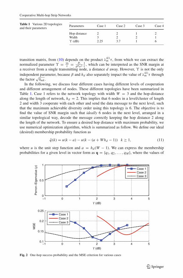
Table 1 Various 2D topologiesand their parameters

Parameters Case 1 Case 2 Case 3 Case 4

Hop distance 2 2 1 2Width 3 2 2 1ϒ (dB) 2.25 3.7 1 6

transition matrix, from (10) depends on the product λ(k)m τ , from which we can extract the

normalized parameter ϒ = γ0τ

= Ptdβσ 2

1τ, which can be interpreted as the SNR margin at

a receiver from a single transmitting node, a distance d away. However, ϒ is not the onlyindependent parameter, because β and hd also separately impact the value of λ

(k)m τ through

the factor√

δmk .In the following, we discuss four different cases having different levels of cooperation

and different arrangement of nodes. These different topologies have been summarized inTable 1. Case 1 refers to the network topology with width W = 3 and the hop-distancealong the length of network, hd = 2. This implies that 6 nodes in a level/cluster of length2 and width 3 cooperate with each other and send the data message to the next level, suchthat the maximum achievable diversity order using this topology is 6. The objective is tofind the value of SNR margin such that ideally 6 nodes in the next level, arranged in asimilar topological way, decode the message correctly keeping the hop distance 2 alongthe length of the network. To ensure a desired hop distance with maximum probability, weuse numerical optimization algorithm, which is summarized as follow. We define our ideal(desired) membership probability function as

q̂(k) = u(k − a) − u(k − (a + W hd − 1)) k ≥ 1, (11)

where u is the unit step function and a = hd(W − 1). We can express the membershipprobabilities for a given level in vector form as q = {q1, q2, . . . , qM }, where the values of

−1 0 1 2 3 4 50

0.5

1

ϒ (dB)

Per

ron−

Eig

enva

lue

(ρ)

−1 0 1 2 3 4 50.1

0.15

0.2

0.25

ϒ (dB)

MS

E

Case 1Case 2Case 3

Case 1Case 2Case 3

Fig. 2 One-hop success probability and the MSE criterion for various cases

123

S. A. Hassan

qk, k ∈ {1, 2, . . . , M} can be found using (7). Then the problem of finding the best ϒ thatensures the desired hop distance with maximum probability can be formulated as

minϒ>0

Ξ = 1

M

∥∥q − q̂∥∥2

. (12)

In other words, to choose the SNR margin that gives a close approximation to (11), minimize(12) over a range of SNR margins. The value of ϒ , where the minimization is achieved,yields a given hd with maximum probability. The one-hop probability of success at that SNRmargin is simply the Perron eigenvalue of the transition matrix.

Figure 2 shows the results obtained by the numerical optimization criteria for differentcases. For Case 1, it can be seen that the optimized SNR margin is 2.25 dB and the respectiveone-hop success probability is 0.9854. This implies that for the given topology, if a hopdistance of 2 is required in the horizontal dimension (keeping the width of the network at 3),an SNR margin of 2.25 dB provides the desired hop distance with a probability of 0.9854.Similarly, for Case 2, a total of 4 nodes cooperate with each other such that the width ofthe network is 2, while the hop distance remains at 2. It can be seen that an increased SNRmargin is required to get the desired hop distance, since the maximum diversity order of thenetwork has reduced to 4 as compared to 6 in Case 1. Hence an additional SNR margin isrequired to get the same hop distance as in Case 1. Case 4 is another example of hop distance2, however the width of the network is 1, which implies a one-dimensional linear network.A further increase in SNR margin can be observed as a consequence of a further reduceddiversity order.

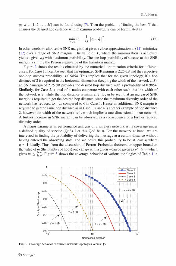
A major parameter in performance analysis of a wireless network is its coverage undera defined quality of service (QoS). Let this QoS be η. For the network at hand, we areinterested in finding the probability of delivering the message at a certain distance withouthaving entered the absorbing state, and we desire this probability to be at least η whereη ∼ 1 ideally. Thus from the discussion of Perron–Frobenius theorem, an upper bound onthe value of m (the number of hops) one can go with a given η can be given as ρm ≥ η, whichgives m ≤ ln η

ln ρ. Figure 3 shows the coverage behavior of various topologies of Table 1 in

100

101

102

0.6

0.65

0.7

0.75

0.8

0.85

0.9

0.95

1

Normalized distance

Qua

lity

of S

ervi

ce (

η)

Case 1Case 2Case 3Case 4

ϒ = 2.25 dB

ϒ = 1 dB ϒ = 3.7 dB

ϒ = 6 dB

Fig. 3 Coverage behavior of various network topologies versus QoS

123

Cooperative Multi-hop Strip Networks

normalized distances versus η, as a function of ϒ . The normalized distance is defined as theproduct of hd and the number of hops (made to reach the destination). It can be seen that Case1 requires a smaller value of SNR margin to reach a larger distance than Case 2 because ofthe difference in topology, although the desired hop distance is the same in both cases. Case1 has 6 nodes in a cluster arranged as (3, 2), whereas Case 2 has 4 nodes in a hop arranged as(2, 2); the ordered pair represents the width, W , and hop distance, hd , as (W, hd). Thus theincreased diversity in Case 1 renders better performance with greater coverage. On the otherhand, Case 4, which is just a one-dimensional linear network requires a larger SNR marginto get a hop distance of 2, however provides the least coverage. This fact can be attributedto the disparate path losses of individual radios that directly impact the performance of theline network. Case 3 requires least SNR margin to get a hop distance of one, since path losseffects are reduced and hence a higher diversity gain is achieved.

5 Conclusion

In this paper, we have shown that the quasi-stationary Markov chain model can be appliedto a 2D grid network and formulated the state space of this system. The behavior of thePerron–Frobenius eigenvalue of the sub-stochastic matrix, referred as the success probability,indicated the level of quality of service that can be achieved for a certain transmission range.We quantified the SNR margin required for various 2D topologies that provide a desired hopdistance. The results showed that for the same hop distance, the larger the number of nodesare in a level, the smaller is the required SNR margin to reach far distances and vice versa.A random 2D modeling of cooperative multi-hop networks, where the position of the nodesis random in a 2D plane, is recommended as a future work.

References

1. Laneman, J. N., Tse, D. N. C., & Wornell, G. W. (2004). Cooperative diversity in wireless networks:Efficient protocols and outage behavior. IEEE Transactions on Information Theory, 50, 3062–3080.

2. Scaglione, A., & Hong, Y. W. (2003). Opportunistic large arrays: Cooperative transmission in wirelessmulti-hop ad hoc networks to reach far distances. IEEE Transactions on Signal Processing, 51(8), 2082–2092.

3. Jung. H, Chang, Y. J., & Ingram, M. A. (2010). Experimental range extension of concurrent cooperativetransmission in indoor environments at 2.4GHz. In Proceedings of military communications conference(MILCOM), San Jose, CA, November 2010.

4. Thanayankizil, L., Kailas, A., & Ingram, M. A. (2009). Routing for wireless sensor networks with anopportunistic large array (OLA) physical layer. Ad Hoc and Sensor Wireless Networks. Special Issue onthe 1st international conference on sensor technologies and applications 2009, 8(1–2): 79–117.

5. Hong, Y. W., & Scaglione, A. (2006). Energy-efficient broadcasting with cooperative transmissions inwireless sensor networks. IEEE Transactions on Wireless Communications, 5(10), 2844–2855.

6. Mergen, B. S., & Scaglione A. (2005). A continuum approach to dense wireless networks with cooperation.In Proceedings of IEEE INFOCOM, March 2005, pp. 2755–2763.

7. Kailas, A., & Ingram, M. A. (2010). Analysis of a simple recruiting method for cooperative routes andstrip networks. IEEE Transactions on Wireless Communications, 9(8), 2415–2419.

8. Jung, H., & Ingram, M. A. (2012). Analysis of intra-flow interference in opportunistic large array trans-mission for strip networks. In Proceedings of IEEE ICC, 2012, pp. 104–108.

9. Capar C., Goeckel D., & Towsley D. F. (2011). Broadcast analysis for large cooperative wireless networks.CoRR abs/1104.3209.

10. Hassan, S. A., & Ingram, M. A. (2011). A quasi-stationary Markov chain model of a cooperative multi-hoplinear network. IEEE Transactions on Wireless Communications, 10(7), 2306–2315.

11. Hassan, S. A., & Ingram, M. A. (2012). Benefit of co-locating groups of nodes in cooperative linenetworks. IEEE Communication Letters, 16(2), 234–237.

123

S. A. Hassan

12. Hassan S. A., & Ingram M. A. (2011). A stochastic approach in modeling cooperative line networks. InProceedings of IEEE wireless communications and networking conference (WCNC), Cancun, Mexico.

13. Hassan, S. A., & Ingram, M. A. (2012). On the modeling of randomized distributed cooperation for linearmulti-hop networks. In Proceedings of IEEE international conference on communications (ICC), Ottawa,Canada.

14. Hassan, S. A. (2013). Range extension using optimal node deployment in linear multi-hop cooperativenetworks. In Proceedings of IEEE radio and wireless symposium (RWS), Austin, TX.

15. Han, B., Li, J., Su, J., & Cao, J. (2012). Self-supported cooperative networking for emergency servicesin multi-hop wireless networks. IEEE Journal on Selected Areas in Communications, 30(2), 450–457.

16. Chang, Y. J., & Ingram, M. A. (2010). Cluster transmission time synchronization for cooperative trans-mission using software defined radio. In IEEE (ICC) workshop on cooperative and cognitive mobile,networks (CoCoNet3), May 2010.

17. Meyer, C. D. (2001). Matrix analysis and applied linear algebra. Philadelphia, PA: SIAM publishers.18. Ross, S. M. (2007). Introduction to probability models. London: Academic Press.

Author Biography

Syed Ali Hassan received his Ph.D. in Electrical Engineering fromGeorgia Institute of Technology, Atlanta, USA in 2011. He receivedhis M.S. Mathematics from Georgia Tech in 2011 and MS Electri-cal Engineering from University of Stuttgart, Germany, in 2007. Hewas awarded BE Electrical Engineering (highest honors) from NationalUniversity of Sciences and Technology (NUST), Pakistan, in 2004. Hisbroader area of research is signal processing for communications. Cur-rently, he is working as an Assistant Professor at the School of Elec-trical Engineering and Computer Science (SEECS), NUST, where heis heading the IPT research group, which focuses on various aspectsof theoretical communications. Prior to joining SEECS, he worked asa research associate at Cisco Systems Inc., CA, USA, where he wasinvolved with the home networking business unit in devising efficientstrategies for home networking. He has chaired several sessions ininternational conferences and has served as a TPC member for IEEETencon 2012, IEEE ICET 2012, and IEEE IEISA 2012.

123