Performance Analysis of Computer Systems...HPCS Performance Targets 8 HPCC was developed by HPCS to...

Holger Brunst ([email protected])

Matthias S. Mueller ([email protected])

Center for Information Services and High Performance Computing (ZIH)

Performance Analysis of Computer Systems

Monitoring Techniques



Summary of Previous Lecture


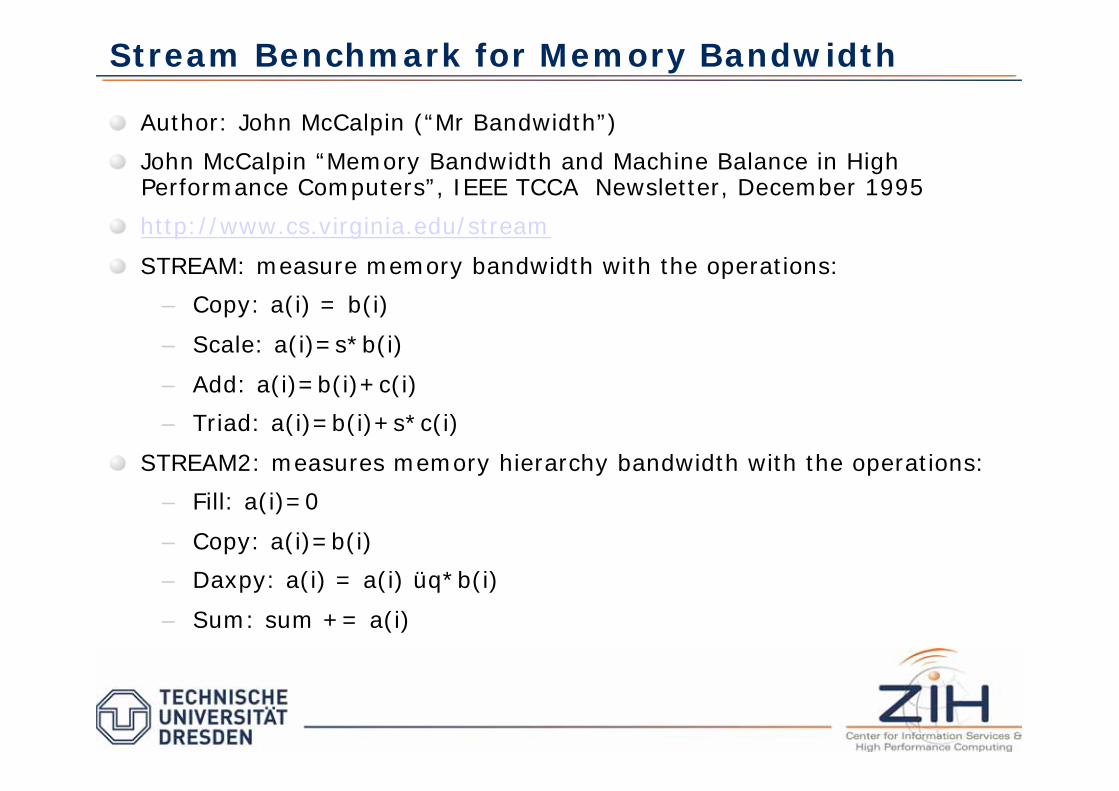
Stream Benchmark for Memory Bandwidth

Author: John McCalpin (“Mr Bandwidth”)

John McCalpin “Memory Bandwidth and Machine Balance in High Performance Computers”, IEEE TCCA Newsletter, December 1995

http://www.cs.virginia.edu/stream

STREAM: measure memory bandwidth with the operations:

– Copy: a(i) = b(i)

– Scale: a(i)=s*b(i)

– Add: a(i)=b(i)+c(i)

– Triad: a(i)=b(i)+s*c(i)

STREAM2: measures memory hierarchy bandwidth with the operations:

– Fill: a(i)=0

– Copy: a(i)=b(i)

– Daxpy: a(i) = a(i) üq*b(i)

– Sum: sum += a(i)

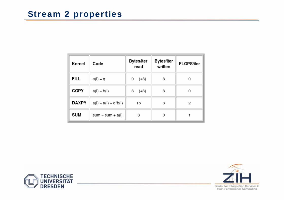
Stream 2 properties

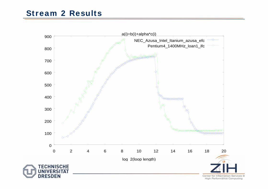
Stream 2 Results

0

100

200

300

400

500

600

700

800

900

0 2 4 6 8 10 12 14 16 18 20

log_2(loop length)

a(i)=b(i)+alpha*c(i)

NEC_Azusa_Intel_Itanium_azusa_efc

Pentium4_1400MHz_loan1_ifc

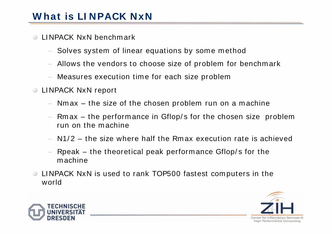
What is LINPACK NxN

LINPACK NxN benchmark

– Solves system of linear equations by some method

– Allows the vendors to choose size of problem for benchmark

– Measures execution time for each size problem

LINPACK NxN report

– Nmax – the size of the chosen problem run on a machine

– Rmax – the performance in Gflop/s for the chosen size problem run on the machine

– N1/2 – the size where half the Rmax execution rate is achieved

– Rpeak – the theoretical peak performance Gflop/s for the machine

LINPACK NxN is used to rank TOP500 fastest computers in the world

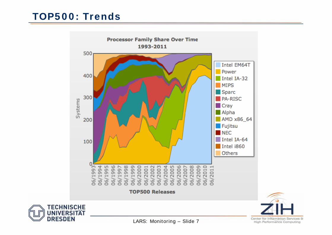
TOP500: Trends

LARS: Monitoring – Slide 7

HPCS Performance Targets

8

HPCC was developed by HPCS to assist in testing new HEC systems Each benchmark focuses on a different part of the memory hierarchy HPCS performance targets attempt to

Flatten the memory hierarchy Improve real application performance Make programming easier

HPC Challenge

Performance Targets

HPL: linear system solve Ax = b

STREAM: vector operations A = B + s * C

FFT: 1D Fast Fourier Transform Z = fft(X)

RandomAccess: integer update T[i] = XOR( T[i], rand)

Cache(s)

Local Memory

Registers

Remote Memory

Disk

Tape

Instructions

Memory Hierarchy

Operands

Lines Blocks

Messages

Pages

Max Relative

8x

40x

200x

64000 GUPS 2000x

2 Pflop/s

6.5 Pbyte/s

0.5 Pflop/s

HPC Challenge Benchmark

Consists of basically 7 benchmarks;

– Think of it as a framework or harness for adding benchmarks of interest.

HPL (LINPACK) MPI Global (Ax = b)

STREAM Local; single CPU

*STREAM Embarrassingly parallel

PTRANS (A A + BT) MPI Global

RandomAccess Local; single CPU

*RandomAccess Embarrassingly parallel

RandomAccess MPI Global

BW and Latency – MPI

FFT - Global, single CPU, and EP

Matrix Multiply – single CPU and EP

Tests on Single Processor and System

Local - only a single processor is performing computations.

Embarrassingly Parallel - each processor in the entire system is performing computations but they do no communicate with each other explicitly.

Global - all processors in the system are performing computations and they explicitly communicate with each other.

Computational

resources

CPU computational

speed

Memory bandwidth

Node

Interconnect bandwidth

HPL

Matrix Multiply

STREAM Random & Natural Ring

Bandwidth & Latency

Computational Resources and HPC Challenge

Memory Access Patterns



When the only tool you have is a hammer,

every problem begins to resemble a nail.

Abraham Maslow


Outline

Motivation

Strategies and terminology

Interval Timers

Program Execution Monitors

Instrumentation


Motivation

A monitor is a tool to observe the activities on a system

Reasons to monitor a system:

– System programmer:

• Find frequently used segments of a program and optimize their performance

– System manager:

• Measure resource utilization and find performance bottleneck(s)

• Tune the system by adjusting system parameters

– System Analyst:

• Use monitor data to characterize the workload for capacity planning

• Find model parameters, validate models, and find model inputs


Monitor Terminology

Event:

– Pre-defined change in the system’s state

– Definition depends on measured metric:

• Memory reference, processor interrupt, application phase, disk access, network message

Profile:

– Aggregated picture of an application program

– Example: Accumulated time spent in each function

Trace:

– A log/sequence of individual events

– Includes event type and important system parameters

Overhead:

– Perturbation induced by the monitor


Monitor Classification

System level at which monitor is implemented:

– Software monitor

– Hardware monitor

– Hybrid monitor

Trigger mechanisms:

– Event-driven

– Sample-driven

Recording:

– Profiling

– Tracing

Displaying ability:

– On-line

– Batch/Post mortem


Trigger Mechanisms: Event-driven

Measure performance only when the pre-selected event occurs

Modify system to observe event

Infrequent events small overhead

Frequent events small overhead

Can significantly alter program behavior

Overhead assessment not easy

Good for tools with low-frequency events

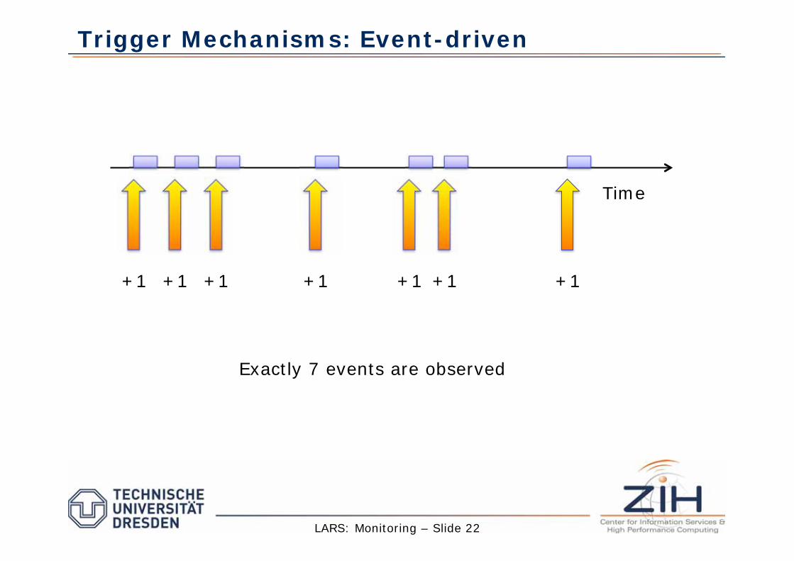
Trigger Mechanisms: Event-driven


T

Time

+1 +1 +1 +1 +1 +1 +1

Exactly 7 events are observed


Trigger Mechanisms: Sample-driven

Measures performance at fixed time intervals

Overhead due to this strategy is independent of the number of times a specific event occurs

Is instead function of the sampling frequency

Not every occurrence of the events will be measured

Sampling produces statistical view on the overall behavior of the

system

Events that occur infrequently may be completely missed

Each run of a sampling-experiment is likely to produce a different result

Trigger Mechanisms: Sample-driven


T

Time

+1 +1 +1

Observes 3 events out of 5 samples

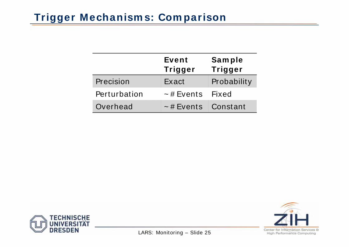
Trigger Mechanisms: Comparison


Event

Trigger

Sample

Trigger

Precision Exact Probability

Perturbation ~#Events Fixed

Overhead ~#Events Constant


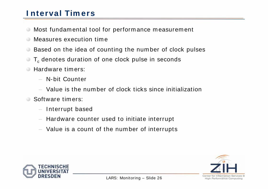
Interval Timers

Most fundamental tool for performance measurement

Measures execution time

Based on the idea of counting the number of clock pulses

Tc denotes duration of one clock pulse in seconds

Hardware timers:

– N-bit Counter

– Value is the number of clock ticks since initialization

Software timers:

– Interrupt based

– Hardware counter used to initiate interrupt

– Value is a count of the number of interrupts

Interval Timers: Quantization Errors

Timer resolution quantization error

Interval timer reports 10 clock ticks:

Interval timer reports 11 clock ticks:

Te is rounded to ± one clock tick: nTc < Te < (n+1) Tc

Rounding is unpredictable

Tc should be as small as possible


Clock

Event

Clock

Event


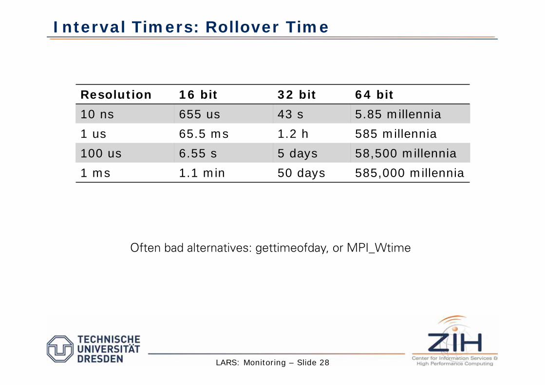
Often bad alternatives: gettimeofday, or MPI_Wtime

Interval Timers: Rollover Time

Resolution 16 bit 32 bit 64 bit

10 ns 655 us 43 s 5.85 millennia

1 us 65.5 ms 1.2 h 585 millennia

100 us 6.55 s 5 days 58,500 millennia

1 ms 1.1 min 50 days 585,000 millennia


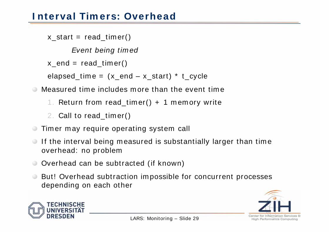
Interval Timers: Overhead

x_start = read_timer()

Event being timed

x_end = read_timer()

elapsed_time = (x_end – x_start) * t_cycle

Measured time includes more than the event time

1. Return from read_timer() + 1 memory write

2. Call to read_timer()

Timer may require operating system call

If the interval being measured is substantially larger than time

overhead: no problem

Overhead can be subtracted (if known)

But! Overhead subtraction impossible for concurrent processes depending on each other


Interval Timers: Measuring Short Intervals

Based on quantization effects, we cannot directly measure events

whose durations are less than the resolution of the timer

We can however make many measurements of a short duration

event to obtain a statistical estimate of the event‘s duration

m = number of times event was observed

n = total number of measurements

Average duration of event is: m/n * Tc

Problem 1: Events need to take place within the timers resolution from time to time

Problem 2: Only average values


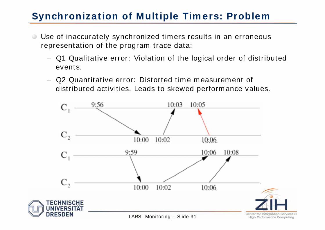
Synchronization of Multiple Timers: Problem

Use of inaccurately synchronized timers results in an erroneous

representation of the program trace data:

– Q1 Qualitative error: Violation of the logical order of distributed

events.

– Q2 Quantitative error: Distorted time measurement of

distributed activities. Leads to skewed performance values.

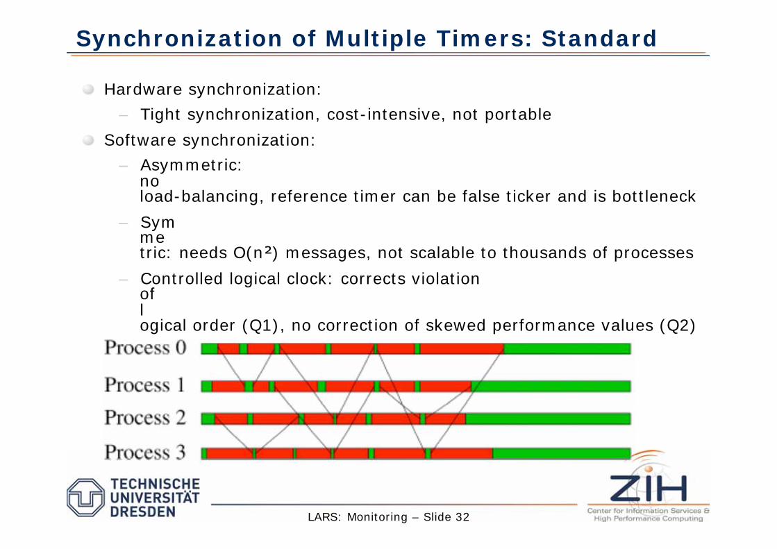
Synchronization of Multiple Timers: Standard

Hardware synchronization:

– Tight synchronization, cost-intensive, not portable

Software synchronization:

– Asymmetric: no load-balancing, reference timer can be false ticker and is bottleneck

– Symmetric: needs O(n ) messages, not scalable to thousands of processes

– Controlled logical clock: corrects violation of logical order (Q1), no correction of skewed performance values (Q2)



Synchronization of Multiple Timers: Goals

Need for a novel timer synchronization

with respect to the requirements of parallel event tracing:

– Load-balanced, low synchronization overhead,

– Portable, scalable and robust synchronization algorithm,

– Restore the relationship of concurrent events,

– Accurate mapping of the event flow for an enhanced performance analysis.


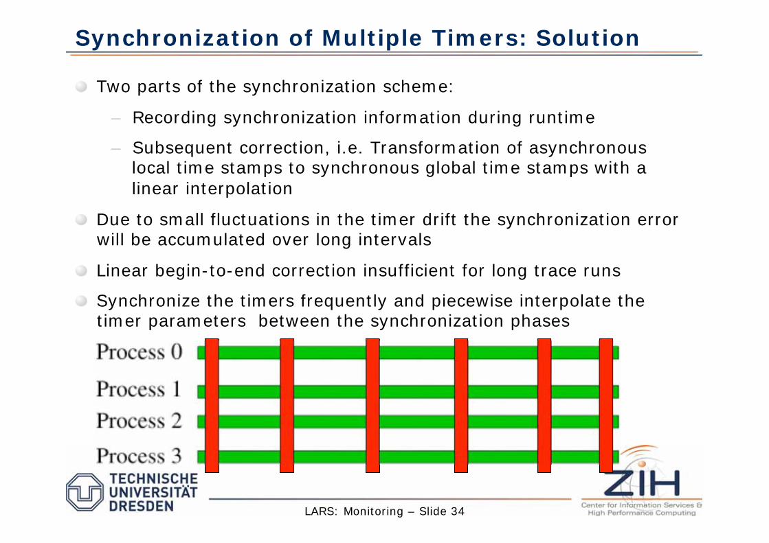
Synchronization of Multiple Timers: Solution

Two parts of the synchronization scheme:

– Recording synchronization information during runtime

– Subsequent correction, i.e. Transformation of asynchronous local time stamps to synchronous global time stamps with a

linear interpolation

Due to small fluctuations in the timer drift the synchronization error will be accumulated over long intervals

Linear begin-to-end correction insufficient for long trace runs

Synchronize the timers frequently and piecewise interpolate the timer parameters between the synchronization phases


Program Monitors: PC Sampling

General statistical measurement technique in which a subset (i.e. a

sample) of the members of a population being examined is selected at random

Information of interest is gathered from the subset of the total population

Assumption: Since the samples were chosen completely at random, the characteristics of the overall population will approximately

follow the same proportion as do the characteristics of the subset actually measured

Profile: Samples are taken at fixed times

Interrupt service routine examines the return address stack to find the address of the instruction/function that was executed


Time

Task 1

Task 2

Task 3

Sample

Program Monitors: PC Sampling


Program Monitors: Basic Block Counting

Produces an exact execution profile by counting the number of times each basic block is executed

Basic block is sequence of processor instructions that has no branches into or out of the sequence

Additional instructions simply count the number of times the block is executed

After termination: values form a histogram

Show how often each block is executed

Complete instruction execution frequency counts can also be obtained from these counts

Key difference between basic block profiling and PC sampling: basic block profiling gives the exact execution frequencies of all instructions

Can add substantial amount of runtime overhead! Average number of instructions varies between three and 20!

Overhead: More instructions, different memory behavior!


Program Monitors: Indirect Strategies

Indirect strategy has to be used if metric is not directly accessible

Try to deduce and derive the desired performance metric from related event which can be measured

Development of an appropriate indirect measurement strategy which minimizes the overhead: difficult, needs experience

Impossible to make any general statements about a measurement tool that makes use of an indirect strategy

Key: match the characteristics of the desired metric with the appropriate measurement strategies


Program Monitors: Tracing

Not only simply recording the fact that the event has happened

Stores some portion of the system state

Instead of keeping just the number of page faults, a tracing record strategy may store the addresses that caused the page fault.

Requires significantly more storage

Time required to save the state can significantly alter program

behavior being measured


Time

Application CPU

1

2

3

4 Application

CPU

Monitor

Application CPU

Monitor

Application CPU

Monitor

Application CPU

Monitor

Application CPU

Monitor 10,000

.

.

.

Monitor

Trace

Data

Trace

Data

Performance Visualization

Enable Scalability?




Profiling: provides summary information

Profiling does not provide any information about the order in which the instructions were executed

Trace:

Dynamic list of the events generated by the program as it executes

Time ordered list of

– all of the instructions executed

– sequences of memory addresses accessed by a program

– sequences of disk blocks referenced by the file system

– sizes and destination of all messages sent over a network



Several difficulties

– Execution-time slowdown

– Other program perturbations by the execution of the additional tracing information

– Volume of data

– Disk speed, organization of the whole process

Advantages:

– Very detailed

– Summarized information can be computed for arbitrary time intervals

– Useful for both performance tuning and debugging

– Easy identification of synchronization issues


Instrumentation

Source-code modification

Software exceptions

Emulation

Microcode modification

Library approach

Compiler modification


Instrumentation: Source Code Modification

Programmer may add additional tracing statements to the source

code manually

Additional program statements will be executed after compilation

Programmer can determine which parts he wants to instrument

Disadvantage:

– Manual approach

– Time consuming

– Error prone

– Programmers mostly believe that they have a clear understanding of the program execution and instrument only

small code areas


Instrumentation: Software Exceptions

Some processors support software exceptions just before the

execution of each instruction

Exception routine can decode the instruction to determine its

operands

Accurate but

– Slowed down execution time by a factor of about 1000

– By far too detailed in most cases


Instrumentation: Emulation

Emulator is a program that makes the system on which it executes

appear to the outside as if it were something completely different

Java Virtual Machine executes application programs written in the

Java programming language by emulating the operation of a processor that implements Java byte-code instructions

Tracing then straight forward, but

– slows down execution significantly

– Not clear how to implement selective tracing


Instrumentation: Library Approach

Parallel programs most often use communication libraries

These libraries can be instrumented easily

Communication is two sided in many cases

Merging results is quite a challenge

Gives quite a good overview about the program behavior


Instrumentation: Compiler Modification

Modify the executable code produced by the compiler

Similar to basic block profiling

Details about the content of the basic block can be obtained from the compiler

Two versions:

– Compilation option

– Post-compilation software tool


TAU

EPILOG

Trace Library

Dynaprof

GCC

IBM

PGI SGI

MPIP

HPCRun

hpcprof

HPMCount

LibHPM

PerfSuite

Intel

TraceCollector

VampirTrace

MPE

(MPICH)

OMPtrace

MPItrace

OPMItrace SCPUs

InfoPerfex

Nanos

Dimemas

TAU

profile

Wallclock

+PAPI Probe

CUBE

gprof

MPIP

HPC Toolkit

HPM Toolkit

PSRUN

pprof

cube

paraprof

xprofiler

HPC View

peekperf

TAU

Trace

EPILOG

VTF

OTF

STF

ALOG

SLOG2

Paraver Paraver

Jumpshot-4

Intel

TraceAnalyzer

Vampir

VNG

Expert

Monitor Analysis Tool Trace Format Profile Format

Tools and Formats: Universe


Tools and Formats: The Format Dilemma

Several parallel trace formats exist

– Different trace formats for different performance systems

• VTF (Vampir), EPILOG (Kojak), SLOG2 (JumpShot-4), TAU

• All public domain

– No real common format or one with special emphasis on scalability

Community has no portable scalable tracing system

– How to support open source and cross-platform tracing tools?

– Mainly concerned with robust analysis and visualization

– Target an open scalable trace format and get community support


Summary

Motivation

Strategies and terminology

Interval Timers

Program Execution Monitors

Instrumentation

Performance Analysis of Computer Systems...HPCS Performance Targets 8 HPCC was developed by HPCS to...

Documents

Transcript of Performance Analysis of Computer Systems...HPCS Performance Targets 8 HPCC was developed by HPCS to...