Performance analysis between a Triathlon and Bicycle helmet

CFD for Engineering Application 7045

MASTER OF MECHANICAL ENGINEERING

Estimate the drag coefficient between a triathlon and a road bicycle helmet

BY

LAVETI TEJASWI A1659176

SANDEEP BOMMAK KUMAR A1671815

LOVEDEEP SINGH A1674234

CHANDRASHNATA DAS A1641362




BY








BY





Contents

1. Introduction .......................................................................................................................................... 3

1. Numerical Methods ..............................................................................................................................4

2. Mesh Details ......................................................................................................................................... 5

3. Boundary conditions .............................................................................................................................7

4. Plots.......................................................................................................................................................8

5.1 Velocity vector ..............................................................................................................................8

5.2 Velocity streamline .......................................................................................................................8

5.3 Y+ Contour .................................................................................................................................... 9

5. Results.................................................................................................................................................10

6. Validation and verification..................................................................................................................12

7. Conclusion...........................................................................................................................................13

8. References ..........................................................................................................................................13

9. Appendix .............................................................................................................................................14

10. Pressure profile ...........................................................................................................................14

1. IntroductionA bicycle helmet is designed to lower the possible impacts to the head of a cyclist which mayoccur in result of an accident. This project investigates an aerodynamically efficient bicyclehelmet which can specifically reduce drag and give a good weight-to-lift ratio. The drag forceplays an important role in the performance of a dynamic body. This aerodynamic drag forcedepends basically on the shape of the body and the drag coefficient.

At a constant velocity, the body having a lower coefficient of drag is expected to have betterperformance than the body having a higher drag coefficient. So, the project mainly focuses onestimating the drag coefficient and then comparing it for all the cases considered, in order tofind out the design with better aerodynamic performance.

In the current project, two different bicycle helmet models are studied and a ComputationalFluid Dynamic (CFD) analysis is done on both the designs to figure out the drag created by eachmodel. The two models considered are Triathlon Bicycle Helmet and a normal bicycle helmet.The overall design of the helmets can be seen in the Figures 1 and 2 and the dimensions of thehelmets are given in the Table 1.

Table 1: Design parameters of two different helmetsLength [mm] Height[mm] Diameter[m]Triathlon helmet 200 150 0.20Road bicycle helmet 200 150 0.20

From a literature review of different research papers of a bicycle helmet, the considered freestream velocity for the particular case is estimated to be around 10 m/s, which is an averagevelocity for riding a bicycle. Furthermore, the maximum velocity taken is 40m/s. Thesevelocities are taken to just analyse the variation caused in drag at different velocity ranges.

Figure1: Traditional bicycle helmet Figure 2: Triathlon helmet

As can be seen, the shapes of the helmets have been simplified for better results duringanalysis. For example, some holes on the surface are neglected which are designed to let the airgo inside the helmet to adjust the temperature for comfort concern. The influence of a humanbody is neglected to make the project much easier.

1. Numerical MethodsThe Numerical methods are applied to solve different governing equations in fluid mechanicsand thermodynamics. These fields are the basic foundation of all CFD models. Henceforth,certain assumptions are considered while formulating these basic equations. Furthermore, thesimplification and discretization of these equations helps to solve the complex flow analysis of acomplex geometry and attain the required solutions for it.

The starting point of any numerical analysis is the governing equations of the problem to besolved. The equations governing the motion of a fluid can be derived from the statements ofthe conservation of mass, momentum, and energy. In the most general form, the fluid motion isgoverned by the time-dependent two-dimensional compressible Navier-Stokes system ofequations.

The following equation is the vector form of Navier-Stokes system:-( ) + ∇ ⃗ = ∆(Γ∇ϕ) + [1]

The differential form of the Navier-Stokes system (Tian, 2015):-( ) + ( ) + ( ) + ( ) = Γ + Γ + Γ + [2]

According to the current project, the flow is assumed to be 2D, steady, and incompressible.Therefore, the given equations can be deduced from these assumptions:

⟶ (−) = 0⟶ = 02D flow⟶ ( ) = 0 and Γ = 0

Using these simplifications, the governing equation becomes:-( ) + ( ) = Γ + Γ + [3]

For the mass continuity equation, = 1, and source term is neglected. Therefore thesimplified continuity equation becomes:- + 0 [4]ϕ = u, v, for the momentum equations in the corresponding direction u, v and Γ becomesΓ = μ and when the viscosity is divided by ρ, it becomes = v, wherev is the kinematic viscosity and the source terms become just the pressure source term, i.e.S = − , S = − simplifying the equations to

Momentum Equation:- + ( ) = + − [5]

Moment Equation:-

( )+ = + − [6]

2. Mesh DetailsThe description of the mesh is as shown in Table 2. A flow field was created around the helmetas shown in Figure 3. To obtain more control over certain areas of the mesh, options likeinflation have been used. A growth rate of 1.2 has also been set to the body sizing option forfurther refinement. The mesh size of the top faces of the helmet is kept to the minimum levelwhile other areas have larger mesh to keep the element size under check.

Table 2: Bicycle helmet mesh details

Domain Nodes Elements Minimumface angle

Maximumface angle

Maximumedgelengthratio

Maximumelementvolumeratio

Connectivityrange

Bicyclehelmet

8170 33681 21.7139[deg] 156.934[deg] 88.3926 34.0572 2-40

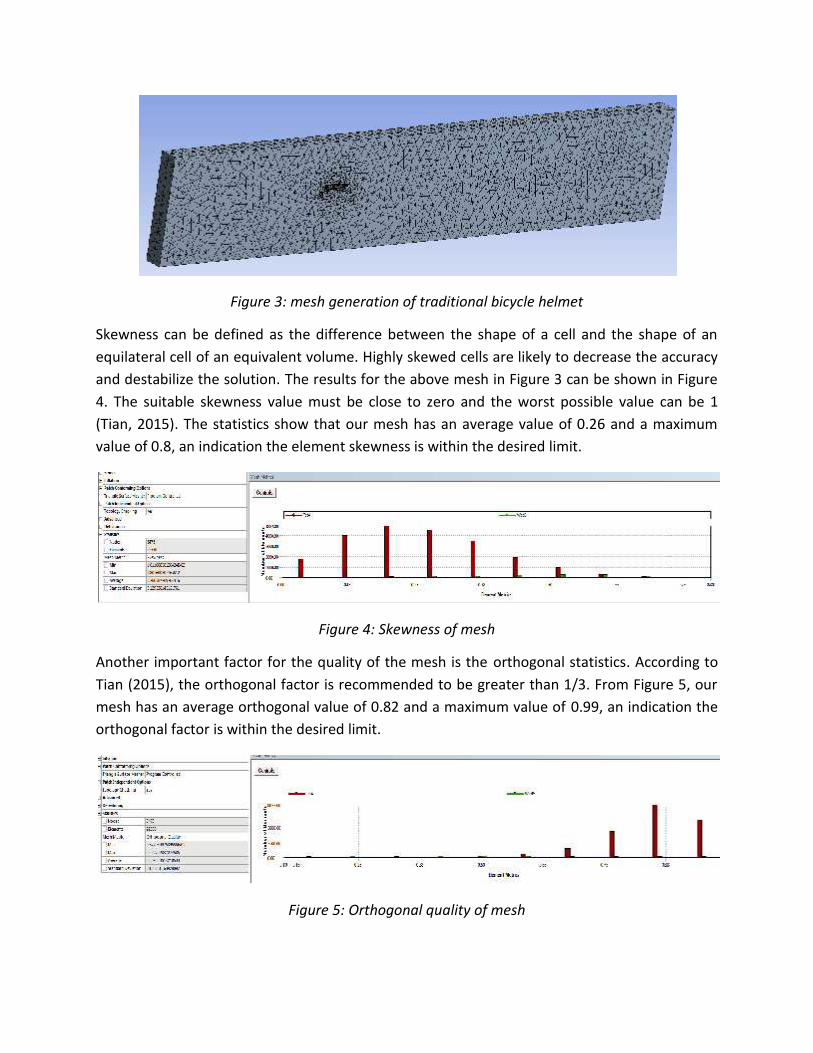
Figure 3: mesh generation of traditional bicycle helmet

Skewness can be defined as the difference between the shape of a cell and the shape of anequilateral cell of an equivalent volume. Highly skewed cells are likely to decrease the accuracyand destabilize the solution. The results for the above mesh in Figure 3 can be shown in Figure4. The suitable skewness value must be close to zero and the worst possible value can be 1(Tian, 2015). The statistics show that our mesh has an average value of 0.26 and a maximumvalue of 0.8, an indication the element skewness is within the desired limit.

Figure 4: Skewness of mesh

Another important factor for the quality of the mesh is the orthogonal statistics. According toTian (2015), the orthogonal factor is recommended to be greater than 1/3. From Figure 5, ourmesh has an average orthogonal value of 0.82 and a maximum value of 0.99, an indication theorthogonal factor is within the desired limit.

Figure 5: Orthogonal quality of mesh

3. Boundary conditionsThe basic boundary conditions are listed in Table 3 along with the boundary type and itscorresponding values.

Table 3: Boundary conditionsBoundary Boundary Type SpecificationsInlet Inlet Speed : 20 [km/hr]

Medium turbulenceSubsonic flow

Outlet Outlet Static pressure: 0 [Pa]Subsonic flow

Sky Opening No slip wallGround Opening No Slip wallHelmet Wall No Slip wall

For the numerical model, a steady state analysis was chosen. This is because to obtain theabsolute value of drag without any time varying parameters. Air was chosen as the materialmedium, taken at 25 °C. The settings for the fluid model were given as ideal gas material, 1[atm] reference pressure, no heat transfer between the surroundings and shear stressturbulence model.

The boundary conditions chosen for this project were inlet, outlet, openings and symmetry asshown in Figure 6. Symmetry boundary conditions were selected because the helmet issymmetrical in nature and a symmetrical flow is expected. Openings are considered because weare not interested with the surroundings or any obstacles in the flow.

Figure 6: Boundary conditions for bicycle helmet

















4. Plots

5.1 Velocity vectorThe velocity vectors for the bicycle helmet are the same as expected. The velocity of air isincreasing across the front or main portion of the helmet and then almost plateaus over themiddle portion of the helmet and then slowly decreases about the tail and rest of the part asshown in Figure 7.

Figure 7: Velocity vector over bicycle helmet

5.2 Velocity streamlineThe velocity streamline plot for the triathlon helmet is quite smooth when compared to that of a bicyclehelmet. Additionally, the velocity vectors for the triathlon helmet are also sharp and tend to stay awayfrom the tail of the helmet as shown in Figure 8. For the traditional bicycle helmet, the velocity vectorsare almost intact to the tail of the helmet and not that smooth as compared to the triathlon helmet asshown in Figure 9.

Figure 8: Velocity streamline on triathlon helmet

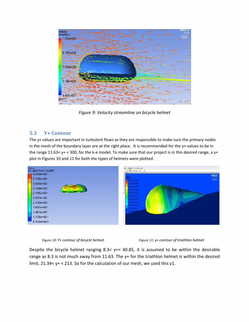
Figure 9: Velocity streamline on bicycle helmet

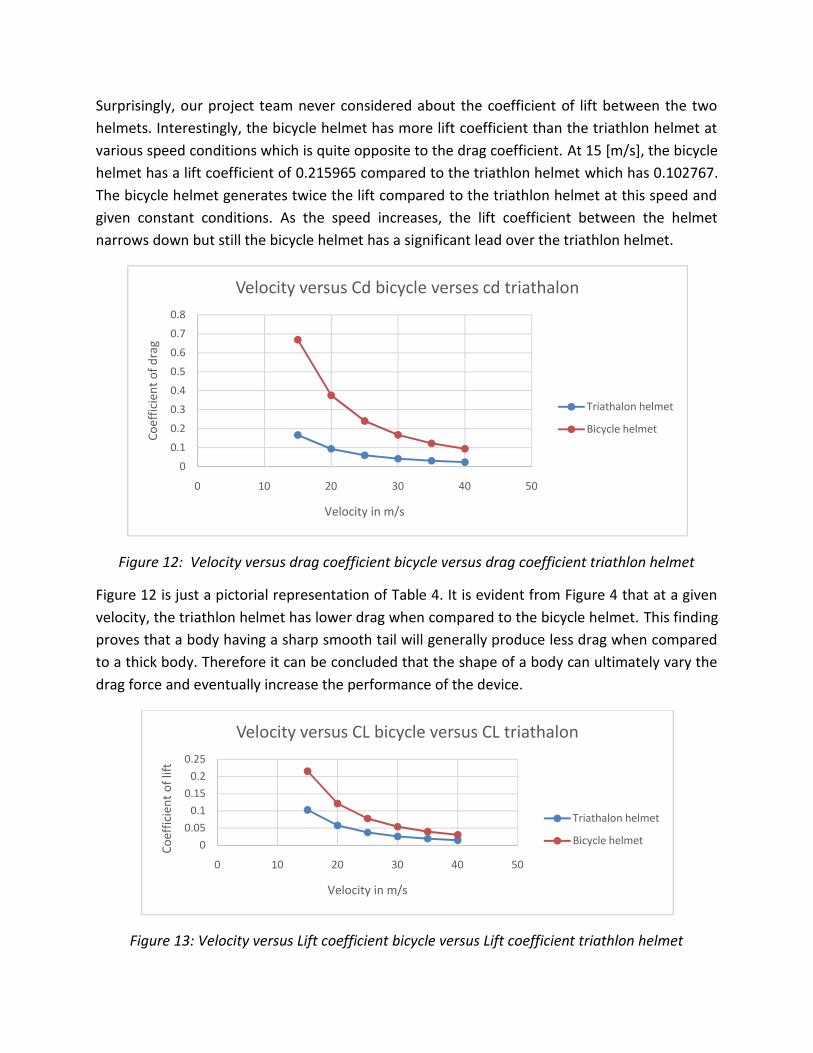
5.3 Y+ ContourThe y+ values are important in turbulent flows as they are responsible to make sure the primary nodesin the mesh of the boundary layer are at the right place. It is recommended for the y+ values to be inthe range 11.63< y+ < 300, for the k-e model. To make sure that our project is in this desired range, a y+plot in Figures 10 and 11 for both the types of helmets were plotted.

Despite the bicycle helmet ranging 8.3< y+< 40.85, it is assumed to be within the desirablerange as 8.3 is not much away from 11.63. The y+ for the triathlon helmet is within the desiredlimit, 21.34< y+ < 213. So for the calculation of our mesh, we used this y1.

Figure 10: Y+ contour of bicycle helmet Figure 11: y+ contour of triathlon helmet

5. ResultsThe main aim of the current project is to investigate the performance between a traditionalbicycle helmet and a triathlon helmet in respect to drag. The drag coefficient can be calculatedfrom the following equation:-

CD = 2 * FD/ ρ * V* Frontal area [7]

As our project adopted a symmetry boundary, the drag force is half of the practical value.Hence, in the calculations, half of the frontal area is considered. The density of air, ρ is set to1.185 [Kg/m3] and the velocity, V is set at 10[m/s]. Furthermore, the velocity is varied from10m/s to 40 m/s and different readings were noted as shown in Table 4 for both the helmets.

Table 4: Comparison of Triathlon versus bicycle helmet in terms of Lift and DragVelocity [m/s] Coefficient of Drag Coefficient of LiftTriathlon Bicycle Triathlon Bicycle15 0.166742 0.668679 0.102767 0.215965

20 0.093792 0.376132 0.057807 0.12148

25 0.060027 0.240724 0.036996 0.077747

30 0.041685 0.16717 0.025692 0.053991

35 0.030626 0.122819 0.018876 0.039667

40 0.023448 0.094033 0.014452 0.03037

As expected, the triathlon helmet has less drag when compared with a bicycle helmet. At 15[m/s] of flow of air, the triathlon helmet had a drag of 0.166742 compared to the bicyclehelmet which generated 0.668679. There is almost 75% reduction in drag between the twohelmets at this speed. More importantly, the helmets are of equal dimensions in terms offrontal area and length.

Consider a scenario, where a bike racer participating in a event chose to opt a bicycle helmetwould eventually be beaten by a rider who wore a triathlon helmet which has less drag andbetter performance. As the velocity increases, the performance between the helmets narrowsdown. At 40 [m/s] the triathlon helmet has a drag of 0.023448 compared to the bicycle helmetwhich has a drag of 0.094033. Despite the gap between the helmets closing down, the triathlonhelmet has a slight advantage in high speeds and large advantage in slow speeds.

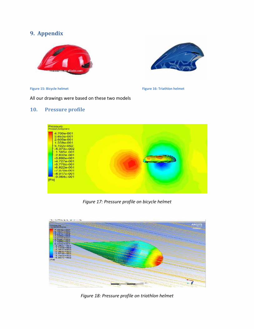
Surprisingly, our project team never considered about the coefficient of lift between the twohelmets. Interestingly, the bicycle helmet has more lift coefficient than the triathlon helmet atvarious speed conditions which is quite opposite to the drag coefficient. At 15 [m/s], the bicyclehelmet has a lift coefficient of 0.215965 compared to the triathlon helmet which has 0.102767.The bicycle helmet generates twice the lift compared to the triathlon helmet at this speed andgiven constant conditions. As the speed increases, the lift coefficient between the helmetnarrows down but still the bicycle helmet has a significant lead over the triathlon helmet.

Figure 12: Velocity versus drag coefficient bicycle versus drag coefficient triathlon helmet

Figure 12 is just a pictorial representation of Table 4. It is evident from Figure 4 that at a givenvelocity, the triathlon helmet has lower drag when compared to the bicycle helmet. This findingproves that a body having a sharp smooth tail will generally produce less drag when comparedto a thick body. Therefore it can be concluded that the shape of a body can ultimately vary thedrag force and eventually increase the performance of the device.

Figure 13: Velocity versus Lift coefficient bicycle versus Lift coefficient triathlon helmet

00.10.20.30.40.50.60.70.8

0 10 20 30 40 50

Coef

ficie

nt o

f dra

g

Velocity in m/s

Velocity versus Cd bicycle verses cd triathalon

Triathalon helmet

Bicycle helmet

00.05

0.10.15

0.20.25

0 10 20 30 40 50

Coef

ficie

nt o

f lift

Velocity in m/s

Velocity versus CL bicycle versus CL triathalon

Triathalon helmet

Bicycle helmet

Figure 13 illustrates the lift coefficient with respect to the two helmets. At a given constantvelocity, the bicycle helmet generates more lift than that off a triathlon helmet. If we had tochoose a body which needs more lift, it is the bicycle helmet and a body which generates lessdrag s the triathlon helmet.

6. Validation and verification

We tried to compare the performance between two differenttypes of helmets as shown in Appendix. One of them is abicycle helmet, which is more oval or round in shape and theother which is blunt or has a leading tail which is sharp, atriathlon helmet. Our model was also draw accordingly tomeet those shapes. However, the dimensions were assumedby our team rather than duplicating the originalspecifications given out by the manufacturer. In the analysis,the two helmets were modelled with the same dimensions soas to predict the most accurate results as possible.

We were not able to find out the accurate value of the dragproduced from these helmets. However, we found out that, atriathlon helmet will have less drag than a bicycle helmet dueto its shape (Kelso, 2014). From figure 14, it can be statedthat a half sphere will be having a drag coefficient of 0.42. Inour project, at velocity 20[m/s], for a bicycle helmet, thecoefficient of drag was found out to be 0.37, which is quiteclose. The bicycle helmet can be considered as a half sphere.

Similarly, from Figure 14, a streamlined half body, which resembles a triathlon helmet, isexpected to have a drag coefficient of 0.09. At a velocity of 20[m/s], in our project, the triathlonhelmet had a drag coefficient of 0.093, which is exact. This validation may not be 100 %accurate due to several assumptions made for the simplification of the project. However, ourmodel is capable of producing reasonable results. A proper validation of the data would bebetter to test these helmets in a wind tunnel conditions.

Our team accept that we were not able to do produce tests such as the Richardsonextrapolation convergence test. Apart from that, our model is providing reasonable results.

Figure 14: Drag coefficient versus Shape

7. ConclusionIt was expected that a triathlon helmet would be having better performance and less dragwhen compared to that of a traditional bicycle helmet. This knowledge was known to us in lastsemester when we undertook the course Applied Aerodynamics taught by Professor RichardKelso.

By Taking the CFD course, we were able to prove our theoretical knowledge and understand alot in the application of CFD. Interestingly, we found out something new which was not knownby any of our team mates. The bicycle helmet generated more lift than a triathlon helmet. Thisis because a bicycle helmet has a low pressure region at the centre of the body.

Furthermore, the shape of the body plays a significant role in reducing or decreasing the dragon a body. This was evident from the fact that the triathlon helmet which resembled a halfstreamline body and a bicycle helmet which resembled a half sphere body had different dragcoefficient profile despite having the same goal, which is the rider from head injury.

But we understood that not only can a helmet protect the person from injury, by changing andtailoring the shape of the helmet can be beneficial in other areas such as sport, by providingbetter performance in terms of speed and competition. CFD is a brilliant tool, sometimes trickyto understand, but provided clear insights for our team in the field of aerodynamics.

8. ReferencesKelso, R. (2014). Applied Aerodynamics.

My Solar Electric Cargo Bike. (n.d.). Retrieved 05 28, 2015, fromhttp://mysolarelectriccargobike.blogspot.com.au/2014/04/bicycle-bodywork-3-of-4-body-shapes.html

Tian, Z. (2015). CFD for Engineering Application.

http://ecx.images-amazon.com/images/I/71LVm9xvklL._SX425_.jpg

http://i01.i.aliimg.com/photo/v2/1900470635_3/new_developed_kids_cycle_helmet_with_LED.jpg

9. Appendix

Figure 15: Bicycle helmet Figure 16: Triathlon helmet

All our drawings were based on these two models

10. Pressure profile

Figure 17: Pressure profile on bicycle helmet

Figure 18: Pressure profile on triathlon helmet

Performance analysis between a Triathlon and Bicycle helmet

Engineering

Transcript of Performance analysis between a Triathlon and Bicycle helmet