Performance Analysis and Comparison of Reduced Common Mode Voltage PWM and Standard PWM

Techniques for Three-Phase Voltage Source Inverters

Emre Ün Ahmet M. Hava Department of Electrical and Electronics Engineering

Middle East Technical University İnönü Bulvarı, 06531 Ankara, TURKEY

un@metu.edu.tr hava@metu.edu.tr

Abstract- This paper investigates the performance characteristics of the reduced common mode voltage (RCMV) PWM methods for three phase voltage source inverters and provides a comparison with the standard PWM methods. PWM methods are reviewed and their pulse patterns and common mode voltage patterns illustrated. The AC output current ripple, DC link input current ripple, and output voltage linearity characteristics of each modulation method are thoroughly investigated by analytical methods and simulations. The analysis leads to important results regarding the practical use of the investigated PWM methods. The paper aids in selection of appropriate PWM methods in drives that have low common mode voltage requirements.

I. INTRODUCTION

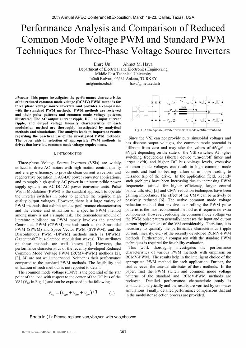
Three-phase Voltage Source Inverters (VSIs) are widely utilized to drive AC motors with high motion control quality and energy efficiency, to provide clean current waveform and regenerative operation in AC-DC power converter applications, and to supply high quality AC power in uninterruptible power supply systems as AC-DC-AC power converter units. Pulse Width Modulation (PWM) is the standard approach to operate the inverter switches in order to generate the required high quality output voltages. However, there is a large variety of PWM methods that exhibit unique performance characteristics and the choice and utilization of a specific PWM method among many is not a simple task. The tremendous amount of literature published on PWM mostly involves the standard Continuous PWM (CPWM) methods such as the Sinusoidal PWM (SPWM) and Space Vector PWM (SVPWM), and the Discontinuous PWM (DPWM) methods such as DPWM1 (2xcenter-60o bus-clamped modulation waves). The attributes of these methods are well known [1]. However, the performance characteristics of the recently developed Reduced Common Mode Voltage PWM (RCMV-PWM) methods [2], [3], [4] are not well understood. Neither is their performance compared to the standard PWM methods. The feasibility and utilization of such methods is not reported to detail. The common mode voltage (CMV) is the potential of the star point of the load with respect to the center of the DC bus of the VSI (Vno in Fig. 1) and can be expressed in the following.

3/)( cnbnanno vvvv ++= (1)

o

−cS

+cS

−bS

+bS+aS

−aS

n

2/dcV

+− a b c

inI

Load

2/dcV

nov

Fig. 1. A three-phase inverter drive with diode rectifier front-end.

Since the VSI can not provide pure sinusoidal voltages and has discrete output voltages, the common mode potential is different from zero and may take the values of ±Vdc/6 or ±Vdc/2 depending on the state of the VSI switches. At higher switching frequencies (shorter device turn-on/off times and larger dv/dt) and higher DC bus voltage levels, excessive common mode voltages can result in high common mode currents and lead to bearing failure or in noise leading to nuisance trip of the drive. In the application field, recently such problems have been increasing due to increasing PWM frequencies (aimed for higher efficiency, larger control bandwidth, etc.) [5] and CMV reduction techniques have been gaining importance. The effect of the CMV can be actively or passively reduced [6]. The active common mode voltage reduction method that involves controlling the PWM pulse patterns is the most economical method as it requires no extra components. However, reducing the common mode voltage via the PWM pulse pattern generally increases the input and output current ripple content of the VSI considerably. Therefore, it is necessary to quantify the performance characteristics (ripple current, linearity, etc.) of the recently developed RCMV-PWM methods. Furthermore, a comparison with the standard PWM techniques is required for feasibility evaluation. This work thoroughly investigates the performance characteristics of various PWM methods with emphasis on RCMV-PWM. The results help in the intelligent choice of the appropriate PWM method for each application. Further, the studies reveal the unusual attributes of these methods. In the paper, first the PWM switch and common mode voltage patterns of the standard and RCMV-PWM methods are reviewed. Detailed performance characteristic study is conducted analytically and the results are verified by computer simulations. Finally, detailed performance comparisons that aid in the modulator selection process are provided.

3030-7803-9547-6/06/$20.00 ©2006 IEEE.

20th Annual APEC Conference&Exposition, March 19-23, Dallas, Texas, USA

Errata in (1): Please replace van,vbn,vcn with vao,vbo,vco

II . SWITCH PULSE AND CMV PATTERNS The performance characteristics of a modulation method are primarily dependent on the modulation index Mi (voltage utilization level) which is defined as follows [1]. stepmmi VVM 611 /= (2) where V1m6step=2Vdc/π and V1m is the magnitude of the reference signal fundamental component. Based on the implementation technique, PWM methods are defined as scalar or Space Vector PWM (SVPWM) methods. In the scalar method a modulation wave is compared with a triangular carrier wave and the intersections define the switching instants. In the space vector approach the reference and inverter voltages are transformed to vectors via the following complex variable transformation. )()3/2( 2

cba VaaVVV ++×= (3) In the above equation 3/2πjea = is the phase shift operator. The vector transformation yields six active and two zero vectors and as shown in Fig. 2 (a), the vectors divide the space into six segments. In the SVPWM method the duty cycles of the voltage vectors are calculated according to the vector volt-seconds balance rule. The sequence of the voltage vectors is selected based on a specified performance criterion such as the switching count and the vectors are programmed accordingly.

A1

B1

A6

A5A4

A3A2

B6B5

B4

B3 B2

)(a )(b

1V0V

6V5V

4V

3V2V

1V

2V3V

4V

5V6V

0V7V7V

Fig. 2. Voltage space vectors and region definitions.

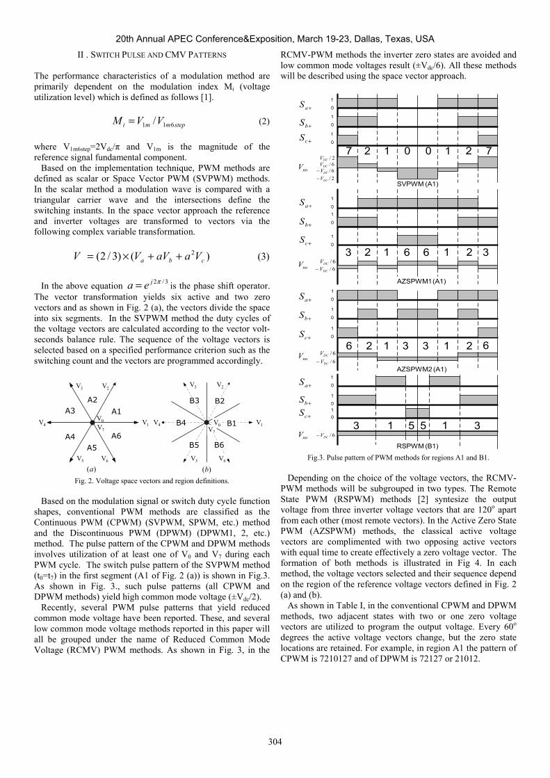
Based on the modulation signal or switch duty cycle function shapes, conventional PWM methods are classified as the Continuous PWM (CPWM) (SVPWM, SPWM, etc.) method and the Discontinuous PWM (DPWM) (DPWM1, 2, etc.) method. The pulse pattern of the CPWM and DPWM methods involves utilization of at least one of V0 and V7 during each PWM cycle. The switch pulse pattern of the SVPWM method (t0=t7) in the first segment (A1 of Fig. 2 (a)) is shown in Fig.3. As shown in Fig. 3., such pulse patterns (all CPWM and DPWM methods) yield high common mode voltage (±Vdc/2). Recently, several PWM pulse patterns that yield reduced common mode voltage have been reported. These, and several low common mode voltage methods reported in this paper will all be grouped under the name of Reduced Common Mode Voltage (RCMV) PWM methods. As shown in Fig. 3, in the

RCMV-PWM methods the inverter zero states are avoided and low common mode voltages result (±Vdc/6). All these methods will be described using the space vector approach.

+aS

+cS+bS

+aS

+cS+bS

+aS

+cS

+bS

+aS

+cS

+bS

noV 6/DCV6/DCV−

6/DCV−

2/DCV−

2/DCV

noV

noV 6/DCV6/DCV−

noV 6/DCV6/DCV−

1

0

1

0

1

0

1

01

0

1

0

1

0

1

0

1

0

1

0

1

010

7 2 2 71 10 0

3 322 11 66

6 622 11 33

33 11 55

(B1) RSPWM

(A1) SVPWM

(A1) AZSPWM1

(A1) AZSPWM2

Fig.3. Pulse pattern of PWM methods for regions A1 and B1.

Depending on the choice of the voltage vectors, the RCMV-PWM methods will be subgrouped in two types. The Remote State PWM (RSPWM) methods [2] syntesize the output voltage from three inverter voltage vectors that are 120o apart from each other (most remote vectors). In the Active Zero State PWM (AZSPWM) methods, the classical active voltage vectors are complimented with two opposing active vectors with equal time to create effectively a zero voltage vector. The formation of both methods is illustrated in Fig 4. In each method, the voltage vectors selected and their sequence depend on the region of the reference voltage vectors defined in Fig. 2 (a) and (b). As shown in Table I, in the conventional CPWM and DPWM methods, two adjacent states with two or one zero voltage vectors are utilized to program the output voltage. Every 60o degrees the active voltage vectors change, but the zero state locations are retained. For example, in region A1 the pattern of CPWM is 7210127 and of DPWM is 72127 or 21012.

304

20th Annual APEC Conference&Exposition, March 19-23, Dallas, Texas, USA

(001)

(010)

(100)

refV

5V

3V 3V

4V

5V 6V

1V

2V

refV

(001)

(010)

(011) (100)

(101)

(110)

1V

Fig. 4. The RSPWM and AZSPWM voltage space vectors.

TABLE I. REGION DEPENDENT PULSE PATTERNS OF VARIOUS PWM METHODS A1 A2 A3 A4 A5 A6

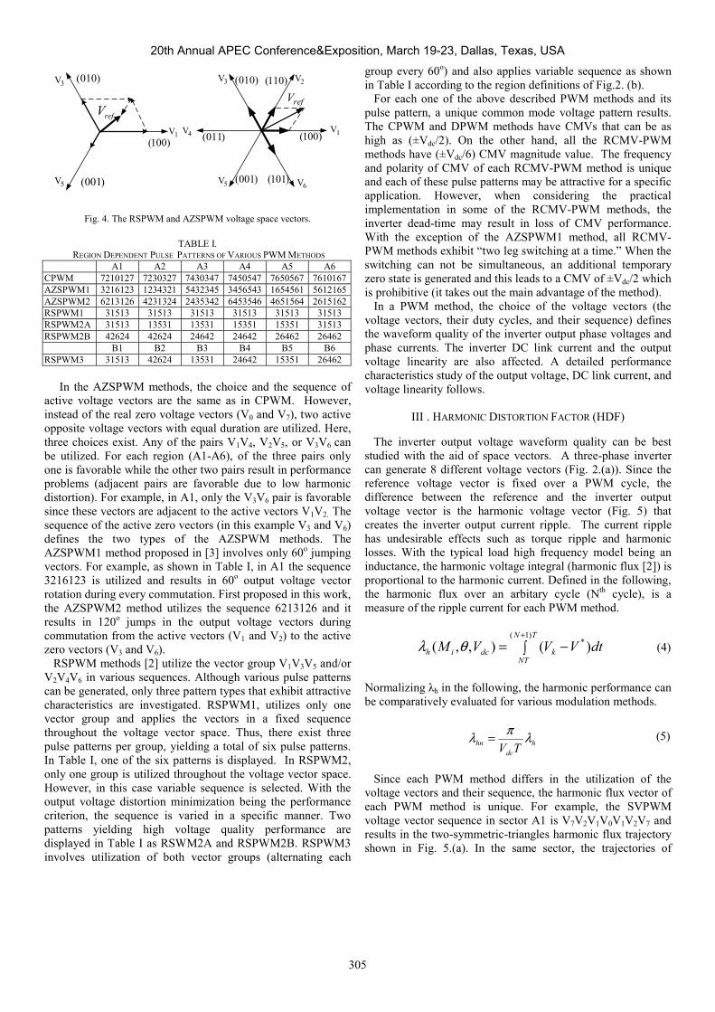
CPWM 7210127 7230327 7430347 7450547 7650567 7610167AZSPWM1 3216123 1234321 5432345 3456543 1654561 5612165AZSPWM2 6213126 4231324 2435342 6453546 4651564 2615162RSPWM1 31513 31513 31513 31513 31513 31513 RSPWM2A 31513 13531 13531 15351 15351 31513 RSPWM2B 42624 42624 24642 24642 26462 26462 B1 B2 B3 B4 B5 B6 RSPWM3 31513 42624 13531 24642 15351 26462 In the AZSPWM methods, the choice and the sequence of active voltage vectors are the same as in CPWM. However, instead of the real zero voltage vectors (V0 and V7), two active opposite voltage vectors with equal duration are utilized. Here, three choices exist. Any of the pairs V1V4, V2V5, or V3V6 can be utilized. For each region (A1-A6), of the three pairs only one is favorable while the other two pairs result in performance problems (adjacent pairs are favorable due to low harmonic distortion). For example, in A1, only the V3V6 pair is favorable since these vectors are adjacent to the active vectors V1V2. The sequence of the active zero vectors (in this example V3 and V6) defines the two types of the AZSPWM methods. The AZSPWM1 method proposed in [3] involves only 60o jumping vectors. For example, as shown in Table I, in A1 the sequence 3216123 is utilized and results in 60o output voltage vector rotation during every commutation. First proposed in this work, the AZSPWM2 method utilizes the sequence 6213126 and it results in 120o jumps in the output voltage vectors during commutation from the active vectors (V1 and V2) to the active zero vectors (V3 and V6). RSPWM methods [2] utilize the vector group V1V3V5 and/or V2V4V6 in various sequences. Although various pulse patterns can be generated, only three pattern types that exhibit attractive characteristics are investigated. RSPWM1, utilizes only one vector group and applies the vectors in a fixed sequence throughout the voltage vector space. Thus, there exist three pulse patterns per group, yielding a total of six pulse patterns. In Table I, one of the six patterns is displayed. In RSPWM2, only one group is utilized throughout the voltage vector space. However, in this case variable sequence is selected. With the output voltage distortion minimization being the performance criterion, the sequence is varied in a specific manner. Two patterns yielding high voltage quality performance are displayed in Table I as RSWM2A and RSPWM2B. RSPWM3 involves utilization of both vector groups (alternating each

group every 60o) and also applies variable sequence as shown in Table I according to the region definitions of Fig.2. (b). For each one of the above described PWM methods and its pulse pattern, a unique common mode voltage pattern results. The CPWM and DPWM methods have CMVs that can be as high as (±Vdc/2). On the other hand, all the RCMV-PWM methods have (±Vdc/6) CMV magnitude value. The frequency and polarity of CMV of each RCMV-PWM method is unique and each of these pulse patterns may be attractive for a specific application. However, when considering the practical implementation in some of the RCMV-PWM methods, the inverter dead-time may result in loss of CMV performance. With the exception of the AZSPWM1 method, all RCMV-PWM methods exhibit “two leg switching at a time.” When the switching can not be simultaneous, an additional temporary zero state is generated and this leads to a CMV of ±Vdc/2 which is prohibitive (it takes out the main advantage of the method). In a PWM method, the choice of the voltage vectors (the voltage vectors, their duty cycles, and their sequence) defines the waveform quality of the inverter output phase voltages and phase currents. The inverter DC link current and the output voltage linearity are also affected. A detailed performance characteristics study of the output voltage, DC link current, and voltage linearity follows.

III . HARMONIC DISTORTION FACTOR (HDF) The inverter output voltage waveform quality can be best studied with the aid of space vectors. A three-phase inverter can generate 8 different voltage vectors (Fig. 2.(a)). Since the reference voltage vector is fixed over a PWM cycle, the difference between the reference and the inverter output voltage vector is the harmonic voltage vector (Fig. 5) that creates the inverter output current ripple. The current ripple has undesirable effects such as torque ripple and harmonic losses. With the typical load high frequency model being an inductance, the harmonic voltage integral (harmonic flux [2]) is proportional to the harmonic current. Defined in the following, the harmonic flux over an arbitary cycle (Nth cycle), is a measure of the ripple current for each PWM method.

∫ −=+ TN

NTkdcih dtVVVM

)1(* )(),,( θλ (4)

Normalizing λh in the following, the harmonic performance can be comparatively evaluated for various modulation methods.

h

dchn TV

λπλ = (5)

Since each PWM method differs in the utilization of the voltage vectors and their sequence, the harmonic flux vector of each PWM method is unique. For example, the SVPWM voltage vector sequence in sector A1 is V7V2V1V0V1V2V7 and results in the two-symmetric-triangles harmonic flux trajectory shown in Fig. 5.(a). In the same sector, the trajectories of

305

20th Annual APEC Conference&Exposition, March 19-23, Dallas, Texas, USA

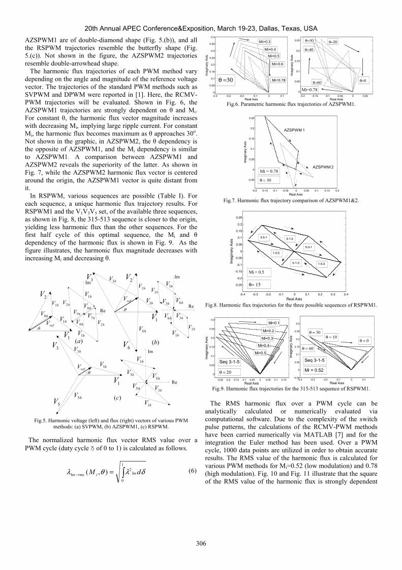
AZSPWM1 are of double-diamond shape (Fig. 5.(b)), and all the RSPWM trajectories resemble the butterfly shape (Fig. 5.(c)). Not shown in the figure, the AZSPWM2 trajectories resemble double-arrowhead shape. The harmonic flux trajectories of each PWM method vary depending on the angle and magnitude of the reference voltage vector. The trajectories of the standard PWM methods such as SVPWM and DPWM were reported in [1]. Here, the RCMV-PWM trajectories will be evaluated. Shown in Fig. 6, the AZSPWM1 trajectories are strongly dependent on θ and Mi. For constant θ, the harmonic flux vector magnitude increases with decreasing Mi, implying large ripple current. For constant Mi, the harmonic flux becomes maximum as θ approaches 30o. Not shown in the graphic, in AZSPWM2, the θ dependency is the opposite of AZSPWM1, and the Mi dependency is similar to AZSPWM1. A comparison between AZSPWM1 and AZSPWM2 reveals the superiority of the latter. As shown in Fig. 7, while the AZSPWM2 harmonic flux vector is centered around the origin, the AZSPWM1 vector is quite distant from it. In RSPWM, various sequences are possible (Table I). For each sequence, a unique harmonic flux trajectory results. For RSPWM1 and the V1V3V5 set, of the available three sequences, as shown in Fig. 8, the 315-513 sequence is closer to the origin, yielding less harmonic flux than the other sequences. For the first half cycle of this optimal sequence, the Mi and θ dependency of the harmonic flux is shown in Fig. 9. As the figure illustrates, the harmonic flux magnitude decreases with increasing Mi and decreasing θ.

refV

2V

hV1

hV2

Im

Re

1Vθ

θ

hV3

hV6

3V

6V

θ

hV5

5V

hV0

refV

1V

2VhV2

hV1

1V

3V

refV

hV3

hV1

hV1

hV2

hV2

hV0

hV7

hV0

hV7

hV1

hV1

hV2

hV2

hV3

hV3

hV6

hV6

hV1

hV1

hV3hV5

hV5

hV1

hV3

Im

Im

Re

Re

)(a )(b

)(c

Fig.5. Harmonic voltage (left) and flux (right) vectors of various PWM

methods: (a) SVPWM, (b) AZSPWM1, (c) RSPWM.

The normalized harmonic flux vector RMS value over a PWM cycle (duty cycle δ of 0 to 1) is calculated as follows.

∫=−

1

0

2),( δλθλ dM hnirmshn (6)

-0.4 -0.3 -0.2 -0.1 0 0.10

0.05

0.1

0.15

0.2

0.25

0.3

0.35

0.4

Real Axis

Imag

inar

y A

xis

Mi=0.78

Mi=0.6

Mi=0.5

Mi=0.4

θ =30

Mi=0.3

-0.2 -0.15 -0.1 -0.05 0 0.05

0

0.05

0.1

0.15

0.2

0.25

Real Axis

Imag

inar

y A

xis

θ=0

θ=20θ=30

θ=40

Mi=0.78θ=60

Fig.6. Parametric harmonic flux trajectories of AZSPWM1.

-0.2 -0.15 -0.1 -0.05 0 0.05 0.1 0.15 0.2

-0.05

0

0.05

0.1

0.15

0.2

0.25

Real Axis

Imag

inar

y A

xis

AZSPWM 1

AZSPWM 2Mi = 0.78

θ = 30

Fig.7. Harmonic flux trajectory comparison of AZSPWM1&2.

-0.4 -0.3 -0.2 -0.1 0 0.1 0.2 0.3 0.4

-0.25

-0.2

-0.15

-0.1

-0.05

0

0.05

0.1

0.15

0.2

0.25

Real Axis

Imag

inar

y A

xis

5-3-1

1-3-5

1-5-3

3-1-5

5-1-3

3-5-1

Mi = 0.5

θ= 15

Fig.8. Harmonic flux trajectories for the three possible sequences of RSPWM1.

-0.25 -0.2 -0.15 -0.1 -0.05 0 0.05 0.1 0.15

0

0.05

0.1

0.15

0.2

0.25

0.3

Real Axis

Imag

inar

y A

xis

Mi=0.4

Mi=0.3

Mi=0.2

Mi=0.1

Seq 3-1-5

θ = 20

Mi=0.5

-0.4 -0.3 -0.2 -0.1 0 0.1-0.05

0

0.05

0.1

0.15

0.2

0.25

0.3

Real Axis

Imag

inar

y Ax

is

θ = 0θ = 10

θ = 30

Seq 3-1-5

Mi = 0.52

θ = 60

Fig.9. Harmonic flux trajectories for the 315-513 sequence of RSPWM1.

The RMS harmonic flux over a PWM cycle can be analytically calculated or numerically evaluated via computational software. Due to the complexity of the switch pulse patterns, the calculations of the RCMV-PWM methods have been carried numerically via MATLAB [7] and for the integration the Euler method has been used. Over a PWM cycle, 1000 data points are utilized in order to obtain accurate results. The RMS value of the harmonic flux is calculated for various PWM methods for Mi=0.52 (low modulation) and 0.78 (high modulation). Fig. 10 and Fig. 11 illustrate that the square of the RMS value of the harmonic flux is strongly dependent

306

20th Annual APEC Conference&Exposition, March 19-23, Dallas, Texas, USA

on θ. At low modulation (Mi=0.52), CPWM methods provide the lowest harmonic flux square-RMS. DPWM methods have larger value. The RCMV-PWM methods have significantly larger distortion than these methods. As Fig.10. illustrates, of the RCMV-PWM methods, AZSPWM2 and RSPWM3 have low distortion, while the other methods have high distortion. AZSPWM1 has poor performance. At high modulation (Mi=0.78), as Fig.11 illustrates, there are striking differences. AZSPWM1 and AZSPWM2 have the two extreme values among all methods. While AZSPWM1 has the worst performance, AZSPWM2 performs the best (near the edges SVPWM is better).

0 1 2 3 4 5 6 70

0.01

0.02

0.03

0.04

0.05

0.06

0.07

0.08

Theta [rad]

La

mb

da

Sq

uar

e

AB ) DPWM 1CD ) DPWM 3AD ) DPWM 2, DPWM MAXCB ) DPWM 0, DPWM MIN

1 ) AZSPWM 12 ) AZSPWM 23 ) RSPWM 1 (3-1-5)4 ) RSPWM 25 ) RSPWM 3

SPWM

SVPWM

A B

C D

3

4

2

1

5

Fig.10. λ2=f(θ) spatial variation for Mi=0.52.

0 0.1 0.2 0.3 0.4 0.5 0.6 0.7 0.8 0.9 1

0.005

0.01

0.015

0.02

0.025

0.03

0.035

Theta [rad]

Lam

bda

Squ

are

A B

C D

1

AZSPWM-1

AZSPWM-2

1 ) SPWMAB ) DPWM 1CD ) DPWM 3AD ) DPWM 2, DPWM MAXCB ) DPWM 0, DPWM MIN

SVPWM

Fig.11. λ2=f(θ) spatial variation for Mi=0.78.

Taking the average value of the local RMS harmonic flux function over the full fundamental cycle (spanning the whole vector space) and scaling it with 288/π2, the Harmonic Distortion Factor (HDF) that is a true measure of AC current ripple RMS value, can be calculated as follows [1]. ∫== −

πθλ

ππ2

0

22 2

1288)( dMfHDF rmshni (7)

The HDF function is only Mi dependent and each PWM method has a unique HDF characteristic. It can be calculated analytically or numerically. Due to the complexity of the switch pulse patterns, the calculations of the RCMV-PWM methods are performed numerically via MATLAB. The integral is calculated with the Euler method and the vector space is spanned with 628 data points for accurate results.

When comparing the HDF characteristics of various PWM methods, equal number of commutations per PWM cycle must be considered. In order to obtain the same number of commutations (per fundamental cycle) in each method, the switching (carrier) frequency of each method must be divided by Kf which is shown in Table II. Thus, the harmonics are scaled with the Kf factor. The square-RMS harmonic flux is scaled with Kf

2 and as a result HDF is also scaled with Kf2.

TABLE II

THE NUMBER OF COMMUTATIONS PER-CYCLE AND Kf

# Commutations Kf CPWM & AZSPWM1 6 1 DPWM 4 2/3 RSPWM 8 4/3 AZSPWM2 10 5/3

As shown in Fig.12, HDF of each method is unique. Over the full linear modulation range, the CPWM and DPWM methods provide lower HDF than the RCMV-PWM methods. Near zero Mi, the difference is in orders of magnitude. However, as Mi increases, the differences rapidly decrease. All RSPWM methods loose voltage linearity at about 0.5-0.6 Mi. At the expiration point of linearity, HDF of these methods is still significantly poorer than the standard methods. Therefore, the HDF of the RSPWM methods is quite inferior to standard PWM. However, AZSPWM methods are linear throughout the inverter hexagon and their HDF performance increases with Mi. For Mi>0.7, the performance of the AZSPWM methods is closely comparable to the standard methods.

0.1 0.2 0.3 0.4 0.5 0.6 0.7 0.8 0.90

0.5

1

1.5

2

2.5

3

3.5

4

4.5

Mi

HD

F

DPWM1

2

3

4

AZSPWM-1

AZSPWM-21 ) SPWM2 ) SVPWM3 ) RSPWM 14 ) RSPWM 25 ) RSPWM 3

5

Fig.12. ΗDF=f(Mi) for various PWM methods.

IV. DC LINK CURRENT HARMONICS

The DC link current of the inverter iin (Fig. 1) is important for DC bus capacitor sizing as the capacitor suppresses all the PWM ripple current. The DC link current ripple of each modulation method is unique and for each method it is a function of Mi and the power factor angle ϕ. In order to compare the DC link current ripple performance of the discussed modulation methods, the ratio of the harmonic RMS value of the dc link current Iinhrms to the inverter AC output fundamental component current RMS value I1rms is evaluated and termed as the DC link current coefficient Kdc.

307

20th Annual APEC Conference&Exposition, March 19-23, Dallas, Texas, USA

0 0.1 0.2 0.3 0.4 0.5 0.6 0.7 0.8 0.90

0.2

0.4

0.6

0.8

1

1.2

1.4

1.6

Mi

Kdc

CPWM-DPWM

RSPWM3 AZSPWM

rmsinhrmsdc IIK 122 /= (8)

For given Mi and ϕ, the RMS DC link current is calculated over a PWM cycle as a function of θ and this result is calculated over 360o to obtain Iinhrms. Then (8) is calculated. For all the methods discussed, (8) is analytically calculated. Kdc for the standard PWM methods is given in [1]. Kdc of RSPWM3 is given in (9). Kdc of other RSPWM methods are similar to that of RSPWM3 and not discussed further. Kdc of all the AZSPWM methods are the same. The formulas are as follows.

ϕπ

ϕπ

22

22

3 cos182cos61 iiRSPWMdc MMK −+= (9)

ϕπ

ϕπ

ϕπ

22

22 cos182cos392cos

2331 ii

AZSPWMdc MMK −+−= (10)

Evaluating Kdc reveals important attributes of the modulators. As Fig. 13 indicates, all methods are ϕ dependent. The RCMV-PWM methods have several times higher DC link current stress than the CPWM and DPWM methods. At low modulation RSPWM and AZSPWM methods exhibit large stress especially at low cosϕ. At higher cosϕ the AZSPWM stress becomes less. At higher modulation the DC link current stress of the AZSPWM methods becomes comparable to the conventional methods due to the expiration of the active zero state duration.

Fig.13. Kdc=f(Mi,cosφ) for various PWM methods.

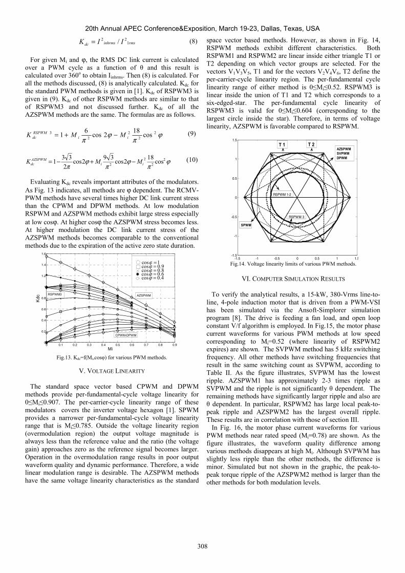
V. VOLTAGE LINEARITY The standard space vector based CPWM and DPWM methods provide per-fundamental-cycle voltage linearity for 0≤Mi≤0.907. The per-carrier-cycle linearity range of these modulators covers the inverter voltage hexagon [1]. SPWM provides a narrower per-fundamental-cycle voltage linearity range that is Mi≤0.785. Outside the voltage linearity region (overmodulation region) the output voltage magnitude is always less than the reference value and the ratio (the voltage gain) approaches zero as the reference signal becomes larger. Operation in the overmodulation range results in poor output waveform quality and dynamic performance. Therefore, a wide linear modulation range is desirable. The AZSPWM methods have the same voltage linearity characteristics as the standard

space vector based methods. However, as shown in Fig. 14, RSPWM methods exhibit different characteristics. Both RSPWM1 and RSPWM2 are linear inside either triangle T1 or T2 depending on which vector groups are selected. For the vectors V1V3V5, T1 and for the vectors V2V4V6, T2 define the per-carrier-cycle linearity region. The per-fundamental cycle linearity range of either method is 0≤Mi≤0.52. RSPWM3 is linear inside the union of T1 and T2 which corresponds to a six-edged-star. The per-fundamental cycle linearity of RSPWM3 is valid for 0≤Mi≤0.604 (corresponding to the largest circle inside the star). Therefore, in terms of voltage linearity, AZSPWM is favorable compared to RSPWM.

-1.5 -1 -0.5 0 0.5 1 1.5-1.5

-1

-0.5

0

0.5

1

1.5

AZSPWMSVPWMDPWM

SPWM

RSPWM 1-2

RSPWM 3

T 1 T 2

Fig.14. Voltage linearity limits of various PWM methods.

VI. COMPUTER SIMULATION RESULTS

To verify the analytical results, a 15-kW, 380-Vrms line-to-line, 4-pole induction motor that is driven from a PWM-VSI has been simulated via the Ansoft-Simplorer simulation program [8]. The drive is feeding a fan load, and open loop constant V/f algorithm is employed. In Fig.15, the motor phase current waveforms for various PWM methods at low speed corresponding to Mi=0.52 (where linearity of RSPWM2 expires) are shown. The SVPWM method has 5 kHz switching frequency. All other methods have switching frequencies that result in the same switching count as SVPWM, according to Table II. As the figure illustrates, SVPWM has the lowest ripple. AZSPWM1 has approximately 2-3 times ripple as SVPWM and the ripple is not significantly θ dependent. The remaining methods have significantly larger ripple and also are θ dependent. In particular, RSPWM2 has large local peak-to-peak ripple and AZSPWM2 has the largest overall ripple. These results are in correlation with those of section III. In Fig. 16, the motor phase current waveforms for various PWM methods near rated speed (Mi=0.78) are shown. As the figure illustrates, the waveform quality difference among various methods disappears at high Mi. Although SVPWM has slightly less ripple than the other methods, the difference is minor. Simulated but not shown in the graphic, the peak-to-peak torque ripple of the AZSPWM2 method is larger than the other methods for both modulation levels.

1cos =ϕ9.0cos =ϕ8.0cos =ϕ6.0cos =ϕ4.0cos =ϕ

308

20th Annual APEC Conference&Exposition, March 19-23, Dallas, Texas, USA

0 0.005 0.01 0.015 0.02 0.025 0.03-80

-60

-40

-20

0

20

40

60

80

t[s]

i [A

]

SVPWM +50A

AZSPWM1 +25A

AZSPWM2

RSPWM2 -25A

RSPWM3 -50A

Fig. 15. Phase current waveforms of various PWM methods for Mi=0.52.

0 0.002 0.004 0.006 0.008 0.01 0.012 0.014 0.016 0.018 0.02-80

-60

-40

-20

0

20

40

60

80

t[s]

i [A

]

AZSPWM2 +30A

AZSPWM1

SVPWM -30A

Fig. 16. Phase current waveforms of various PWM methods for Mi=0.78.

VII. PERFORMANCE COMPARISONS

The performance study results of the paper are summarized in Table III. The table indicates that in general, RCMV-PWM methods increase the stress on both the AC and DC side of the inverter. Only AZSPWM1 exhibits comparable HDF and Kdc performance to standard methods at high Mi. Therefore, in applications requiring low CMV and operating at high Mi the AZSPWM1 method is favorable. Also motor drives with large leakage inductance that can tolerate the PWM ripple voltage/current may utilize the method throughout the operating range and benefit from the low CMV.

If possible, in some cases the standard methods and the CMV methods can be combined for optimal overall performance. For example, utilizing SVPWM in the low modulation range, and AZSPWM1 in the high modulation range yields superior overall performance. However, the CMV performance at low modulation index remains inferior and requires a cure.

VIII. CONCLUSIONS

This paper investigated the performance characteristics of the RCMV-PWM methods and provided a comparison to the standard PWM methods. The RCMV-PWM methods were classified, their pulse-patterns defined, and new RCMV-PWM methods proposed. Analytical and computer simulation based methods were utilized to obtain the DC link current and AC output voltage and current ripple characteristics. The results illustrate that the standard methods have less DC link and AC output current ripple than the RCMV-PWM methods. As an exceptional case the AZSPWM1 method exhibits superior overall performance at high modulation index. The analysis leads to important conclusions regarding the practical utilization of the investigated PWM methods. The paper aids in selection of appropriate PWM methods in drives that have low common mode voltage requirements.

REFERENCES

[1] A.M. Hava, R.J. Kerkman, T.A. Lipo, “Simple analytical and graphical methods for carrier-based PWM-VSI drives,” IEEE Trans. on Power Electronics, vol. 14, no: 1, pp. 49 – 61. Jan. 1999.

[2] M. Cacciato, A. Consoli, G. Scarcella, A. Testa, “Reduction of common-mode currents in PWM inverter motor drives,” IEEE Trans. on Ind. Applicats., vol. 35, no 2, pp. 469 – 476. March-April 1999.

[3] Y.S. Lai, F.S. Shyu, “Optimal common-mode voltage reduction PWM technique for inverter control with consideration of the dead-time effects-part I: basic development,” IEEE Trans. on Ind. Applicats., vol 40, no. 6, pp.1605 – 1612. Nov.-Dec. 2004.

[4] Y.S. Lai, P.S. Chen, H.K. Lee, J. Chou, “Optimal common-mode voltage reduction PWM technique for inverter control with consideration of the dead-time effects-part II: applications to IM drives with diode front end,” IEEE Trans. on Ind. Applicats. , vol. 40, no 6, pp. 1613 – 1620. Nov.-Dec. 2004.

[5] J.M. Erdman, R.J. Kerkman, D.W. Schlegel, and G.L. Skibinski, “Effect of PWM inverters on AC motor bearing currents and shaft voltages,” IEEE Trans. Ind. Applicat., vol. 32, pp. 250-259, Mar./Apr. 1996.

[6] S. Ogasawara and H. Akagi, “Modeling and damping of high-frequency leakage currents in PWM inverter-fed AC motor drive systems,” Conf. Rec. IEEE-IAS Annu. Meeting, pp. 29-36, Oct. 8–12, 1995.

[7] MATLAB 6.5, Mathworks Inc., 2002. [8] Ansoft Simplorer, V7.0, 2004.

TABLE III

PERFORMANCE COMPARISON OF VARIOUS PWM METHODS

SVPWM DPWM AZSPWM1 AZSPWM2 RSPWM Kdc ( High Mi) Low Low Moderate (low PF dependency) NA Kdc ( Low Mi) Low Low Moderate @ high PF and higher @ low PF High

HDF ( High Mi) Low Low Moderate Moderate NA

HDF ( Low Mi) Low Low High Highest High Switching # per T 6 4 6 10 8

Voltage linearity 0.91 0.91 0.91 0.91 0.52 or 0.60 CMV ( vno) High High Low Low Low

309

20th Annual APEC Conference&Exposition, March 19-23, Dallas, Texas, USA