Perfectly Competitive Markets
56
Perfectl y Competit ive Markets Chapter 9
description
Chapter 9. Perfectly Competitive Markets. Chapter Nine Overview. Introduction Perfect Competition Defined The Profit Maximization Hypothesis The Profit Maximization Condition Short Run Equilibrium Short Run Supply Curve for the Firm Short Run Market Supply Curve - PowerPoint PPT Presentation
Transcript of Perfectly Competitive Markets
Perfectly Competitive
Markets
Chapter 9
2
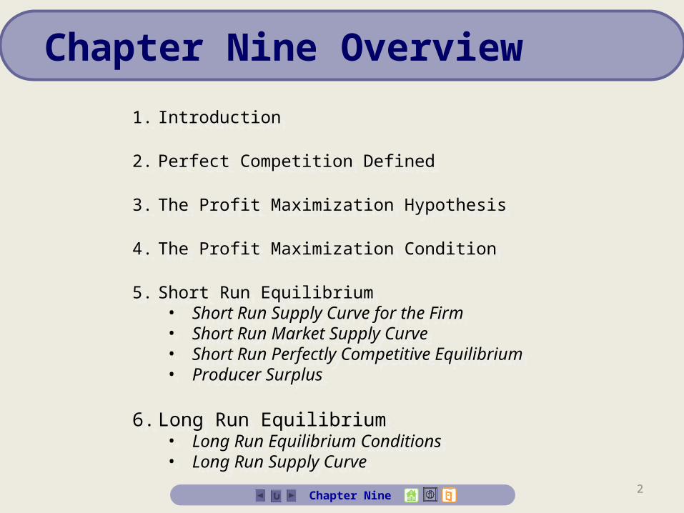
Chapter Nine Overview
1. Introduction
2. Perfect Competition Defined
3. The Profit Maximization Hypothesis
4. The Profit Maximization Condition
5. Short Run Equilibrium• Short Run Supply Curve for the Firm• Short Run Market Supply Curve• Short Run Perfectly Competitive Equilibrium• Producer Surplus
6. Long Run Equilibrium• Long Run Equilibrium Conditions• Long Run Supply Curve
Chapter Nine
3Chapter Nine
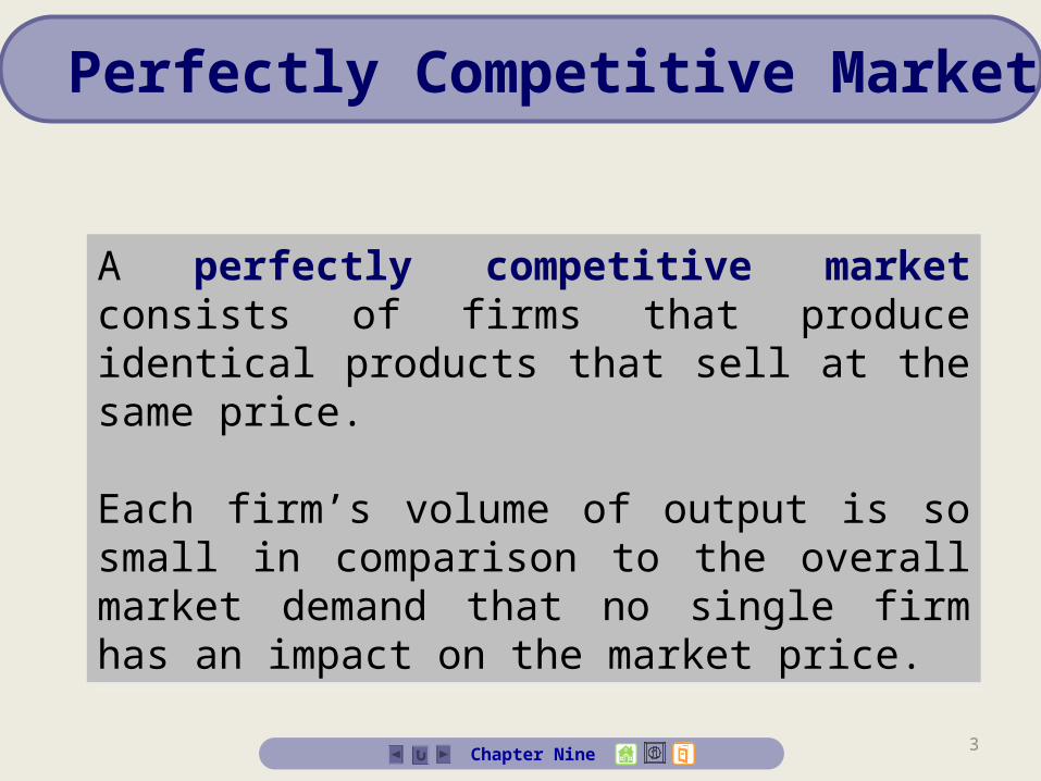
A perfectly competitive market consists of firms that produce identical products that sell at the same price.
Each firm’s volume of output is so small in comparison to the overall market demand that no single firm has an impact on the market price.
A perfectly competitive market consists of firms that produce identical products that sell at the same price.
Each firm’s volume of output is so small in comparison to the overall market demand that no single firm has an impact on the market price.
Perfectly Competitive Markets
4Chapter Nine
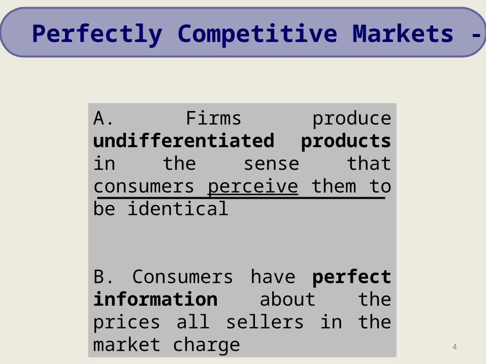
A. Firms produce undifferentiated products in the sense that consumers perceive them to be identical
B. Consumers have perfect information about the prices all sellers in the market charge
A. Firms produce undifferentiated products in the sense that consumers perceive them to be identical
B. Consumers have perfect information about the prices all sellers in the market charge
Perfectly Competitive Markets - Conditions
5Chapter Nine
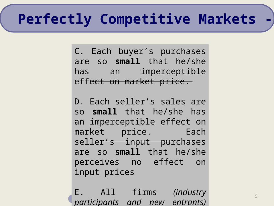
C. Each buyer’s purchases are so small that he/she has an imperceptible effect on market price.
D. Each seller’s sales are so small that he/she has an imperceptible effect on market price. Each seller’s input purchases are so small that he/she perceives no effect on input prices
E. All firms (industry participants and new entrants) have equal access to resources (technology, inputs).
Perfectly Competitive Markets - Conditions
6Chapter Nine
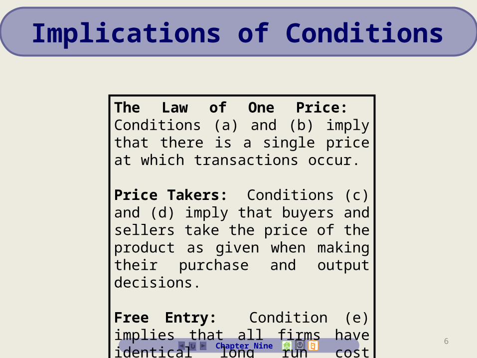
Implications of Conditions
The Law of One Price: Conditions (a) and (b) imply that there is a single price at which transactions occur.
Price Takers: Conditions (c) and (d) imply that buyers and sellers take the price of the product as given when making their purchase and output decisions.
Free Entry: Condition (e) implies that all firms have identical long run cost functions
7Chapter Nine
The Profit Maximization Hypothesis
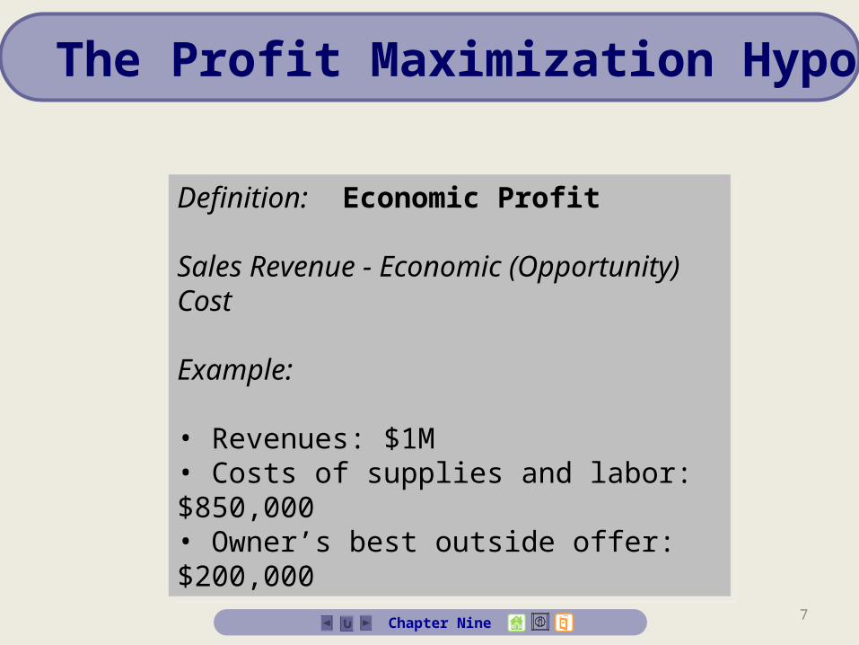
Definition: Economic Profit
Sales Revenue - Economic (Opportunity) Cost
Example:
• Revenues: $1M• Costs of supplies and labor: $850,000• Owner’s best outside offer: $200,000
Definition: Economic Profit
Sales Revenue - Economic (Opportunity) Cost
Example:
• Revenues: $1M• Costs of supplies and labor: $850,000• Owner’s best outside offer: $200,000
8Chapter Nine
The Profit Maximization Hypothesis
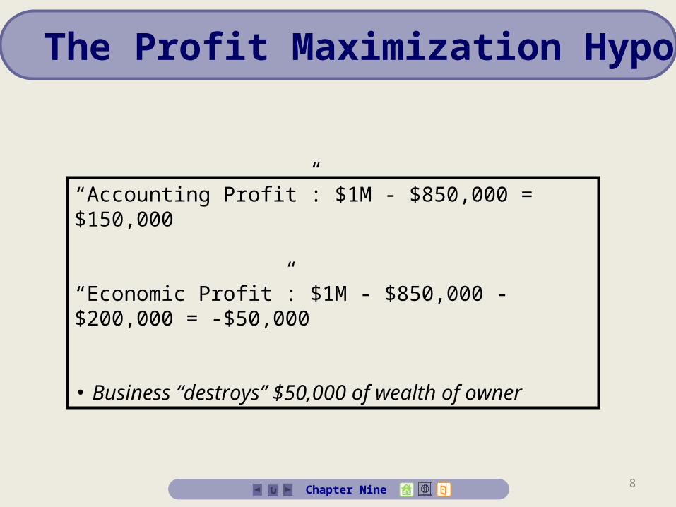
“Accounting Profit”: $1M - $850,000 = $150,000
“Economic Profit”: $1M - $850,000 - $200,000 = -$50,000
• Business “destroys” $50,000 of wealth of owner
9Chapter Nine
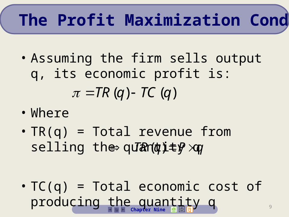
The Profit Maximization Condition
• Assuming the firm sells output q, its economic profit is:
• Where• TR(q) = Total revenue from selling the
quantity q
• TC(q) = Total economic cost of producing the quantity q
)()( qTCqTR
qPqTR )(
10Chapter Nine
The Profit Maximization Condition
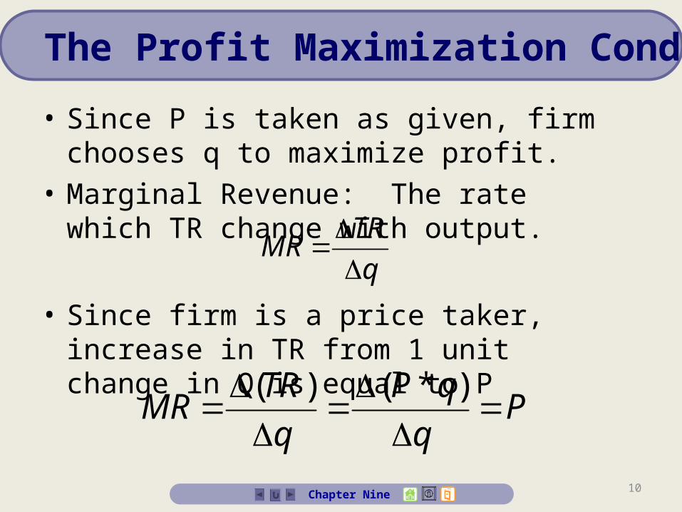
• Since P is taken as given, firm chooses q to maximize profit.
• Marginal Revenue: The rate which TR change with output.
• Since firm is a price taker, increase in TR from 1 unit change in Q is equal to P
q
TRMR
Pq
qP
q
TRMR
)*()(
11Chapter Nine
The Profit Maximization Condition
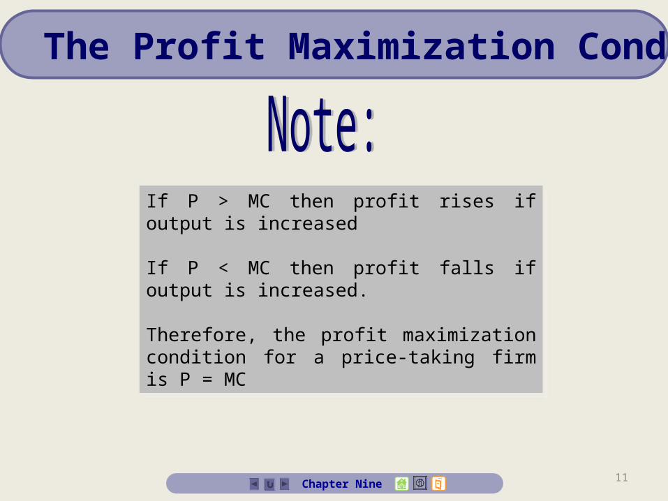
If P > MC then profit rises if output is increased
If P < MC then profit falls if output is increased.
Therefore, the profit maximization condition for a price-taking firm is P = MC
If P > MC then profit rises if output is increased
If P < MC then profit falls if output is increased.
Therefore, the profit maximization condition for a price-taking firm is P = MC

12Chapter Nine
The Profit Maximization Condition
13Chapter Nine
The Profit Maximization Condition
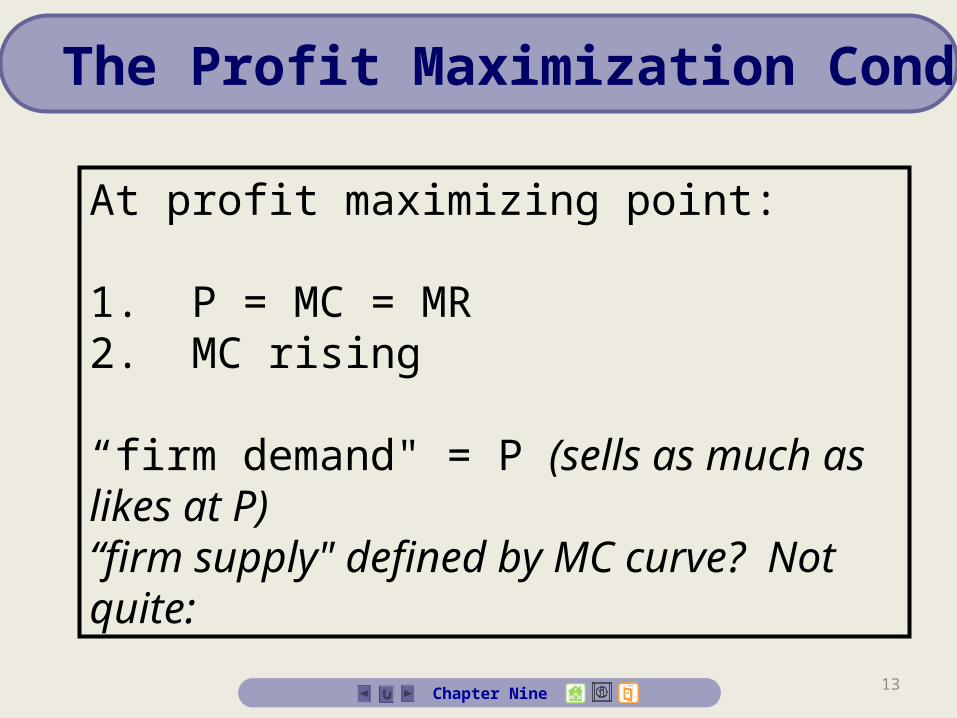
At profit maximizing point:
1. P = MC = MR2. MC rising
“firm demand" = P (sells as much as likes at P)“firm supply" defined by MC curve? Not quite:
14Chapter Nine
Short Run Equilibrium
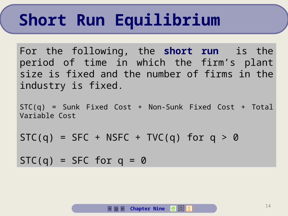
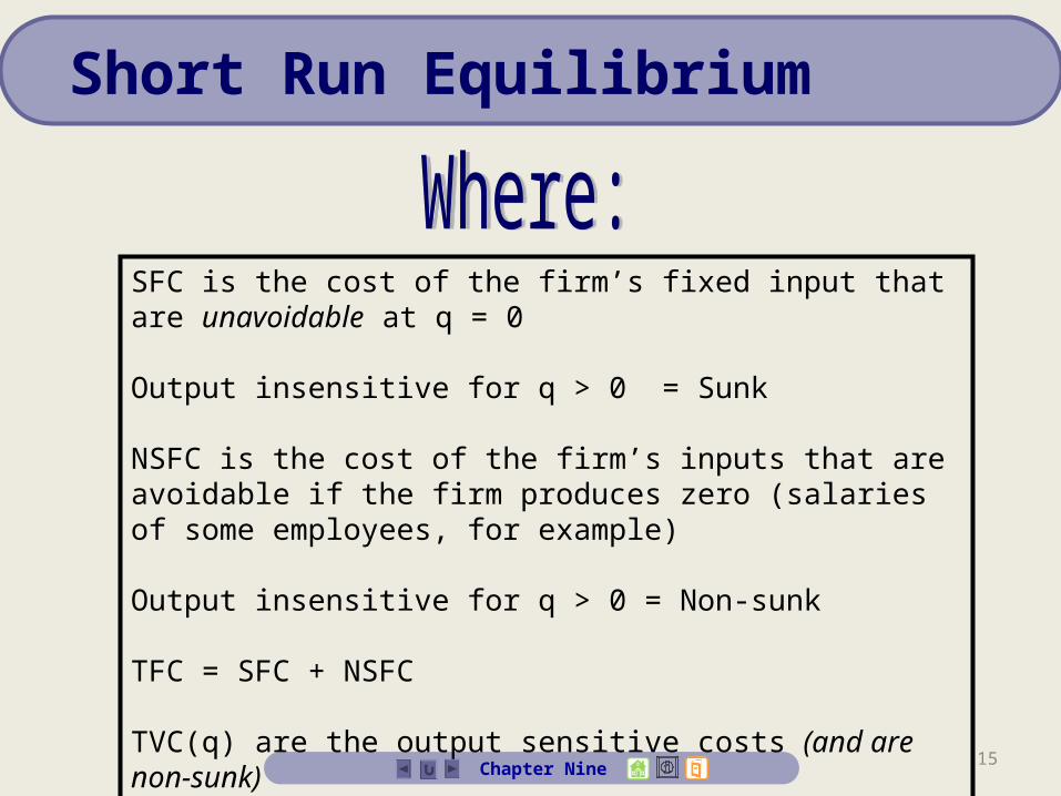
For the following, the short run is the period of time in which the firm’s plant size is fixed and the number of firms in the industry is fixed.
STC(q) = Sunk Fixed Cost + Non-Sunk Fixed Cost + Total Variable Cost
STC(q) = SFC + NSFC + TVC(q) for q > 0
STC(q) = SFC for q = 0
For the following, the short run is the period of time in which the firm’s plant size is fixed and the number of firms in the industry is fixed.
STC(q) = Sunk Fixed Cost + Non-Sunk Fixed Cost + Total Variable Cost
STC(q) = SFC + NSFC + TVC(q) for q > 0
STC(q) = SFC for q = 0
15Chapter Nine
Short Run Equilibrium
SFC is the cost of the firm’s fixed input that are unavoidable at q = 0
Output insensitive for q > 0 = Sunk
NSFC is the cost of the firm’s inputs that are avoidable if the firm produces zero (salaries of some employees, for example)
Output insensitive for q > 0 = Non-sunk
TFC = SFC + NSFC
TVC(q) are the output sensitive costs (and are non-sunk)
16Chapter Nine
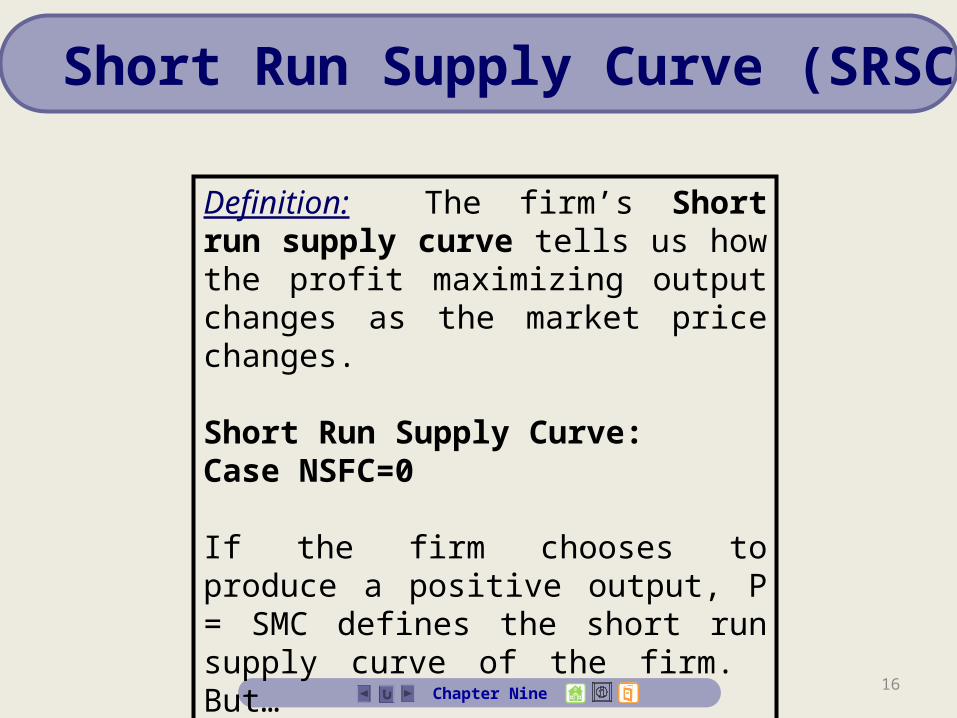
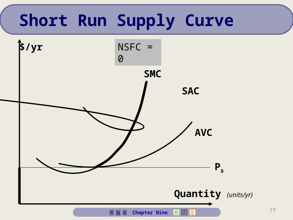
Short Run Supply Curve (SRSC)
Definition: The firm’s Short run supply curve tells us how the profit maximizing output changes as the market price changes.
Short Run Supply Curve: Case NSFC=0
If the firm chooses to produce a positive output, P = SMC defines the short run supply curve of the firm. But…
17Chapter Nine
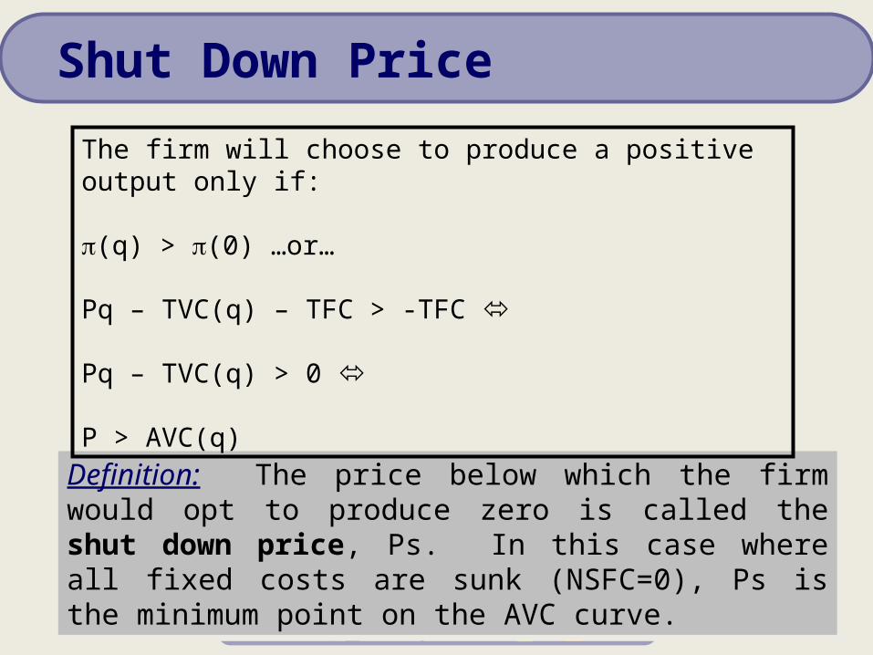
Definition: The price below which the firm would opt to produce zero is called the shut down price, Ps. In this case where all fixed costs are sunk (NSFC=0), Ps is the minimum point on the AVC curve.
Definition: The price below which the firm would opt to produce zero is called the shut down price, Ps. In this case where all fixed costs are sunk (NSFC=0), Ps is the minimum point on the AVC curve.
The firm will choose to produce a positive output only if:
(q) > (0) …or…
Pq – TVC(q) – TFC > -TFC
Pq – TVC(q) > 0
P > AVC(q)
Shut Down Price
18Chapter Nine
Short Run Supply Function
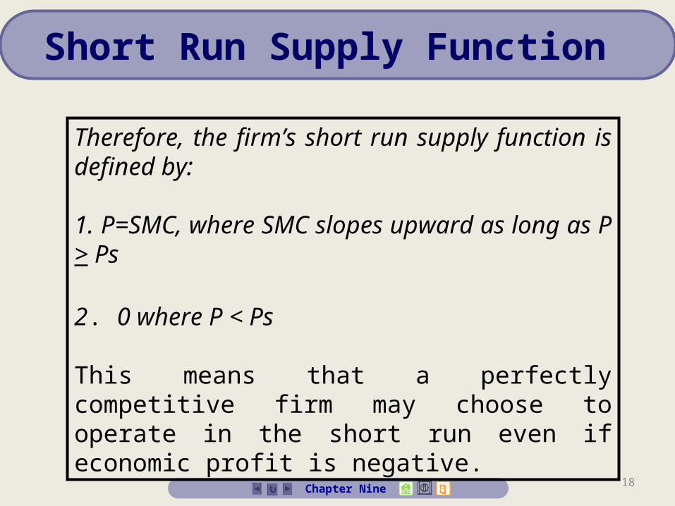
Therefore, the firm’s short run supply function is defined by:
1. P=SMC, where SMC slopes upward as long as P > Ps
2. 0 where P < Ps
This means that a perfectly competitive firm may choose to operate in the short run even if economic profit is negative.
19
NSFC = 0NSFC = 0
Quantity (units/yr)
$/yr
AVC
SAC
SMC
Ps
Chapter Nine
Short Run Supply Curve
20Chapter Nine
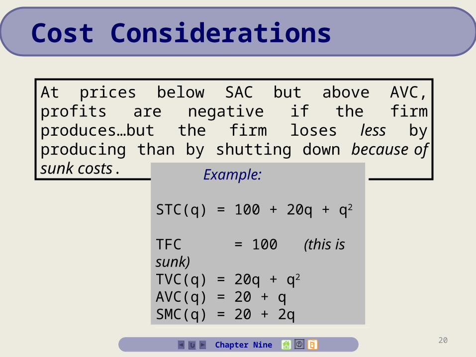
Cost Considerations
At prices below SAC but above AVC, profits are negative if the firm produces…but the firm loses less by producing than by shutting down because of sunk costs.
Example:
STC(q) = 100 + 20q + q2
TFC = 100 (this is sunk)TVC(q) = 20q + q2
AVC(q) = 20 + qSMC(q) = 20 + 2q
Example:
STC(q) = 100 + 20q + q2
TFC = 100 (this is sunk)TVC(q) = 20q + q2
AVC(q) = 20 + qSMC(q) = 20 + 2q
21Chapter Nine
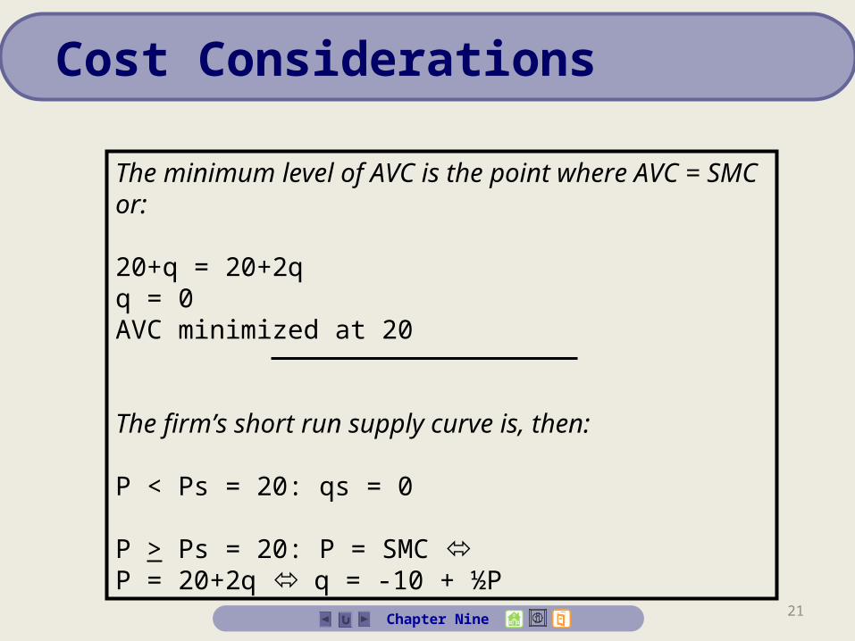
Cost Considerations
The minimum level of AVC is the point where AVC = SMC or:
20+q = 20+2qq = 0 AVC minimized at 20
The firm’s short run supply curve is, then:
P < Ps = 20: qs = 0
P > Ps = 20: P = SMC P = 20+2q q = -10 + ½P
22Chapter Nine
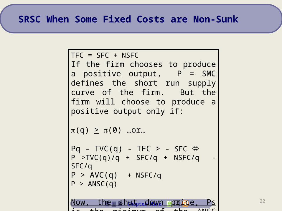
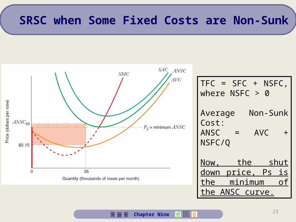
SRSC When Some Fixed Costs are Non-Sunk
TFC = SFC + NSFC If the firm chooses to produce a positive output, P = SMC defines the short run supply curve of the firm. But the firm will choose to produce a positive output only if:
(q) > (0) …or…
Pq – TVC(q) - TFC > - SFC P >TVC(q)/q + SFC/q + NSFC/q - SFC/qP > AVC(q) + NSFC/q P > ANSC(q)
Now, the shut down price, Ps is the minimum of the ANSC curve
23Chapter Nine
SRSC when Some Fixed Costs are Non-Sunk
TFC = SFC + NSFC, where NSFC > 0
Average Non-Sunk Cost:ANSC = AVC + NSFC/Q
Now, the shut down price, Ps is the minimum of the ANSC curve.
24Chapter Nine
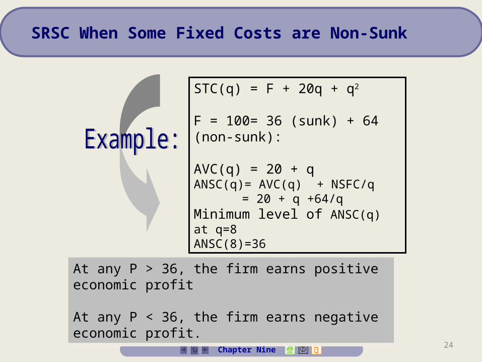
SRSC When Some Fixed Costs are Non-Sunk
STC(q) = F + 20q + q2
F = 100= 36 (sunk) + 64 (non-sunk):
AVC(q) = 20 + qANSC(q)= AVC(q) + NSFC/q
= 20 + q +64/qMinimum level of ANSC(q) at q=8ANSC(8)=36
At any P > 36, the firm earns positive economic profit
At any P < 36, the firm earns negative economic profit.
At any P > 36, the firm earns positive economic profit
At any P < 36, the firm earns negative economic profit.
25Chapter Nine
Market Supply and Equilibrium
Definition: The market supply at any price is the sum of the quantities each firm supplies at that price.
The short run market supply curve is the horizontal sum of the individual firm supply curves.
Definition: The market supply at any price is the sum of the quantities each firm supplies at that price.
The short run market supply curve is the horizontal sum of the individual firm supply curves.
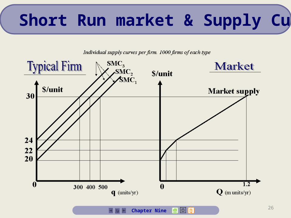
26Chapter Nine
Short Run market & Supply Curves
27Chapter Nine
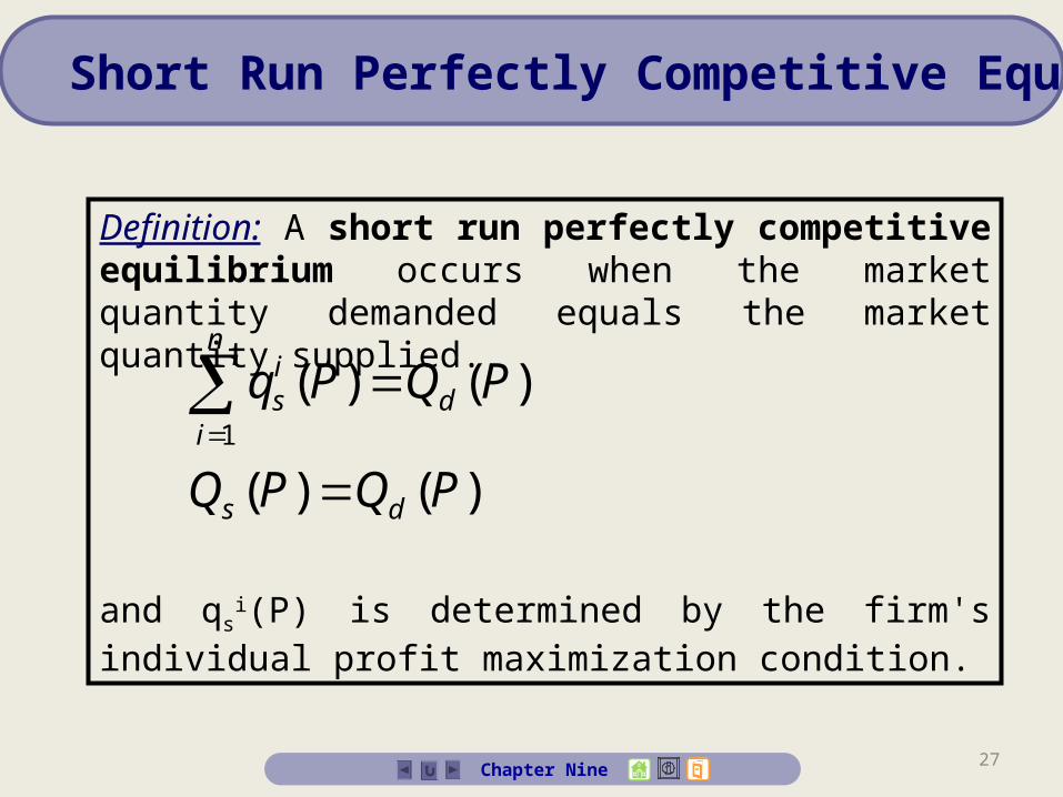
Short Run Perfectly Competitive Equilibrium
Definition: A short run perfectly competitive equilibrium occurs when the market quantity demanded equals the market quantity supplied.
and qsi(P) is determined by the firm's individual profit
maximization condition.
)()(
)()(1
PQPQ
PQPq
ds
d
n
i
is
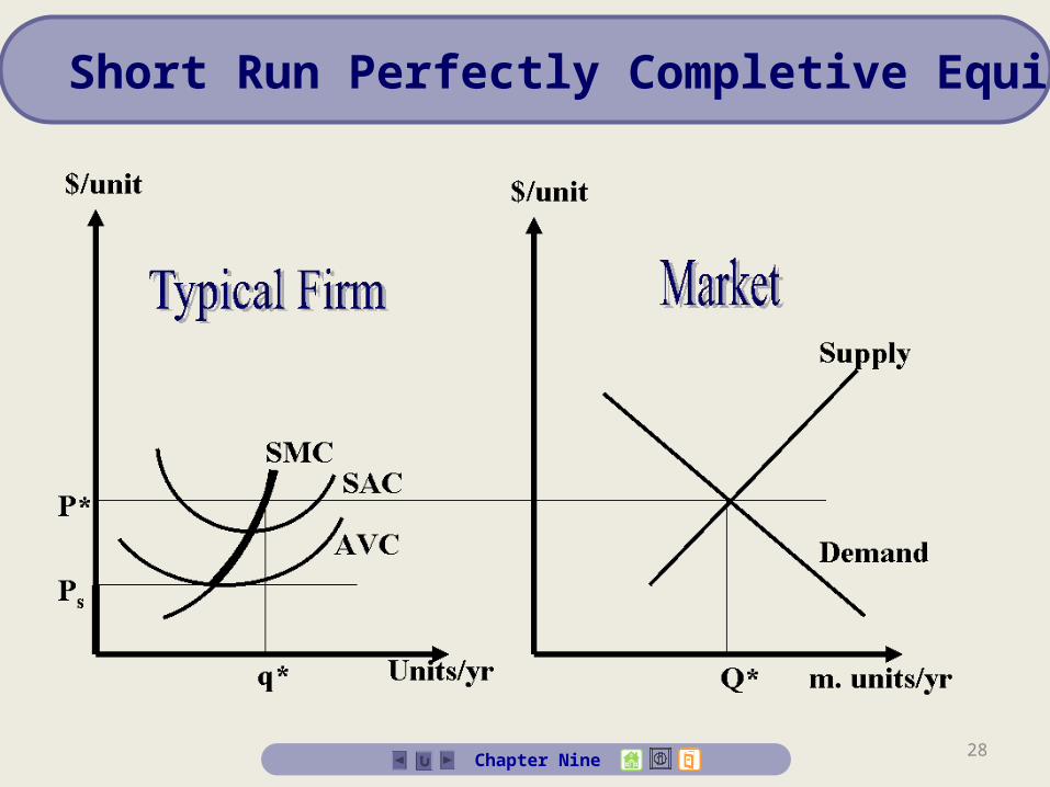
28Chapter Nine
Short Run Perfectly Completive Equilibrium
29Chapter Nine
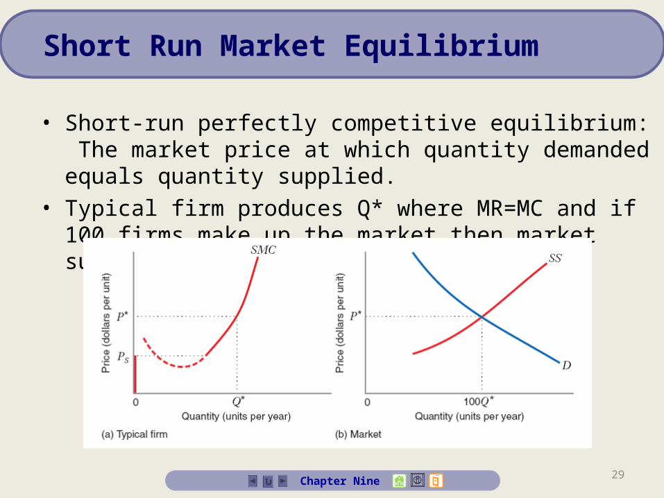
Short Run Market Equilibrium
• Short-run perfectly competitive equilibrium: The market price at which quantity demanded equals quantity supplied.
• Typical firm produces Q* where MR=MC and if 100 firms make up the market then market supply must equal 100Q*
30
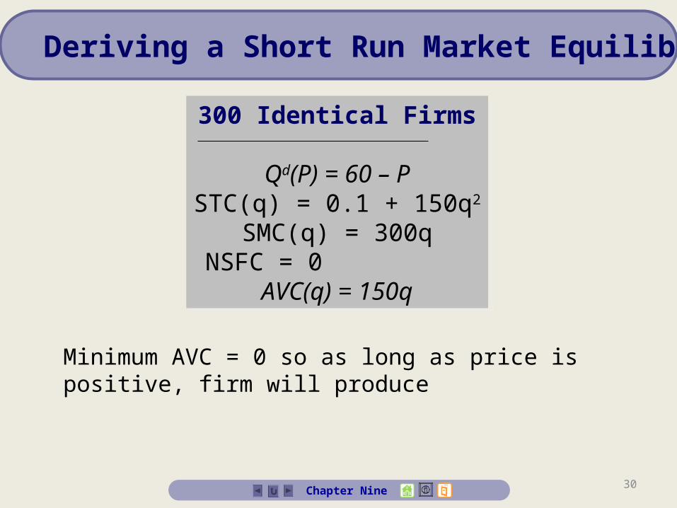
300 Identical Firms
Qd(P) = 60 – PSTC(q) = 0.1 + 150q2
SMC(q) = 300qNSFC = 0 AVC(q) = 150q
300 Identical Firms
Qd(P) = 60 – PSTC(q) = 0.1 + 150q2
SMC(q) = 300qNSFC = 0 AVC(q) = 150q
Chapter Nine
Deriving a Short Run Market Equilibrium
Minimum AVC = 0 so as long as price is positive, firm will produce
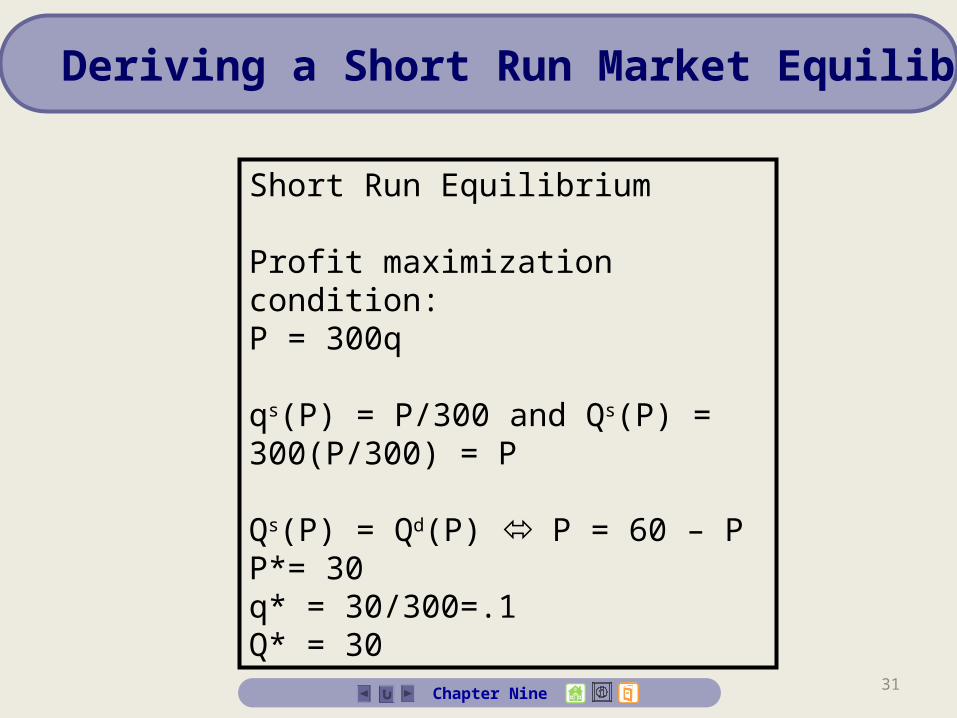
31Chapter Nine
Short Run Equilibrium
Profit maximization condition: P = 300q
qs(P) = P/300 and Qs(P) = 300(P/300) = P
Qs(P) = Qd(P) P = 60 – PP*= 30q* = 30/300=.1Q* = 30
Deriving a Short Run Market Equilibrium
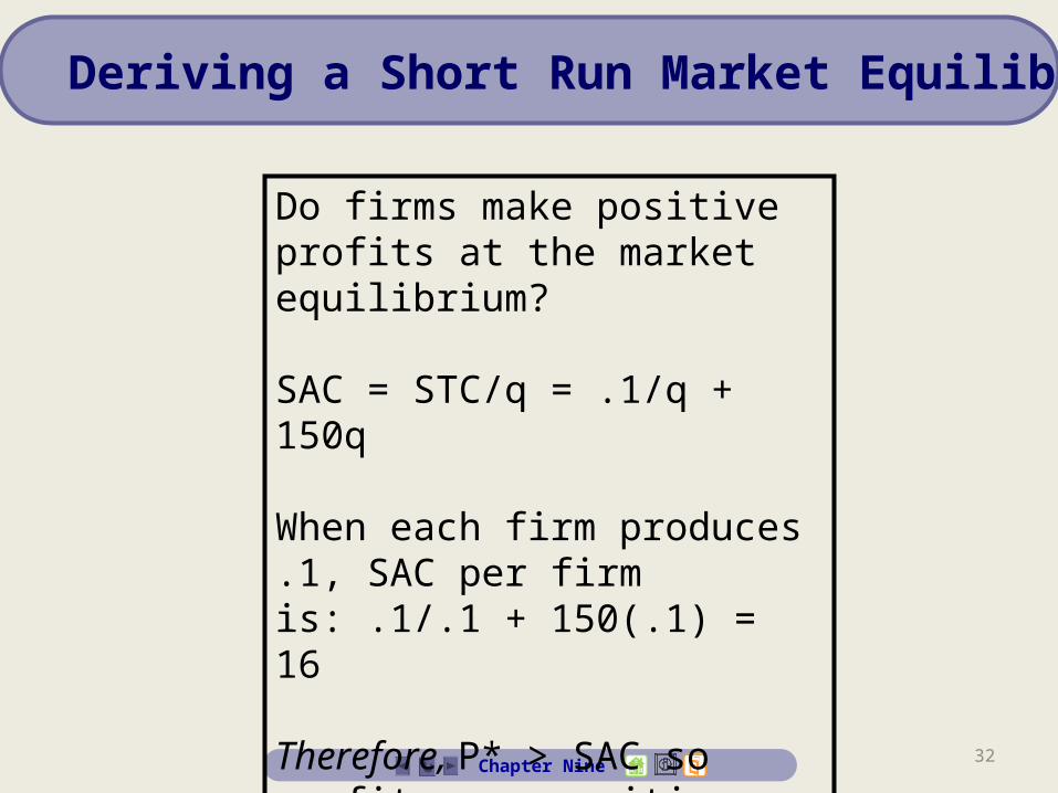
32Chapter Nine
Deriving a Short Run Market Equilibrium
Do firms make positive profits at the market equilibrium?
SAC = STC/q = .1/q + 150q
When each firm produces .1, SAC per firm is: .1/.1 + 150(.1) = 16
Therefore, P* > SAC so profits are positive
33Chapter Nine
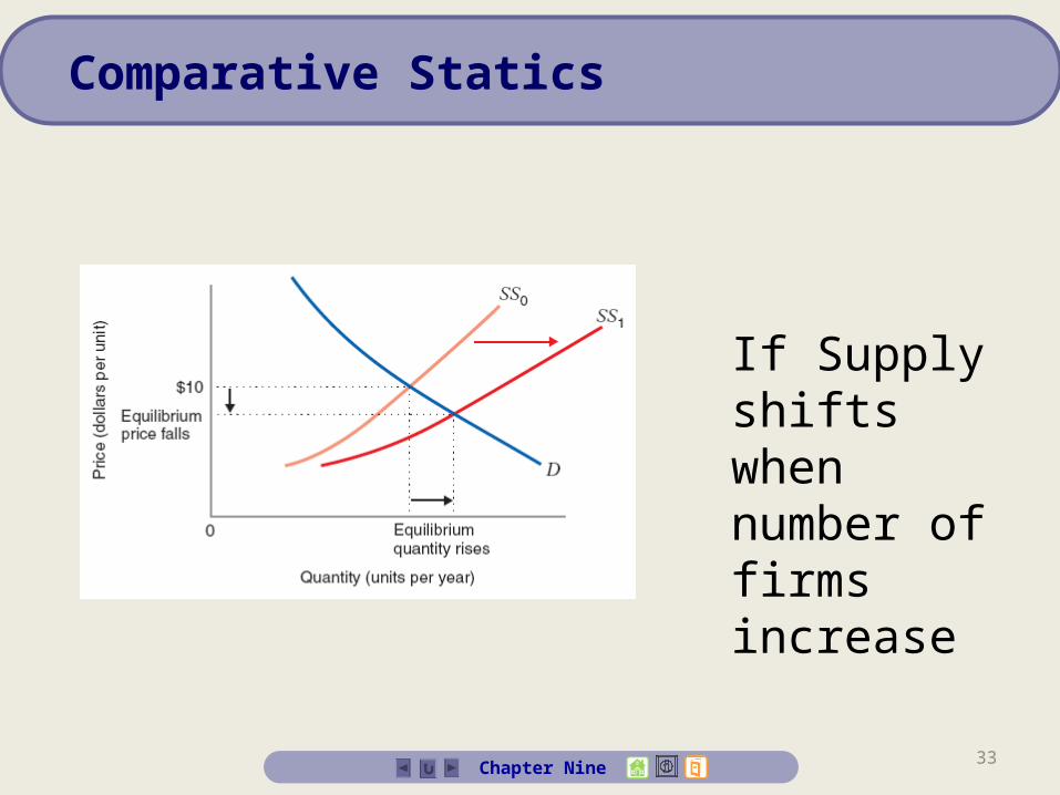
Comparative Statics
If Supply shifts when number of firms increase
34Chapter Nine
Comparative Statics
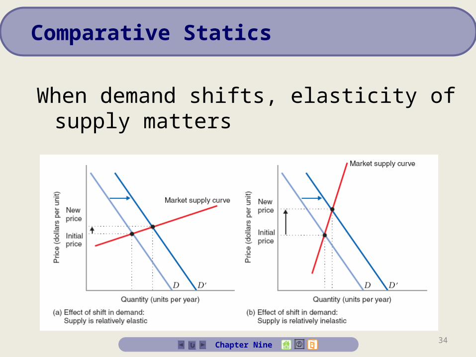
When demand shifts, elasticity of supply matters
35Chapter Nine
Long Run Market Equilibrium
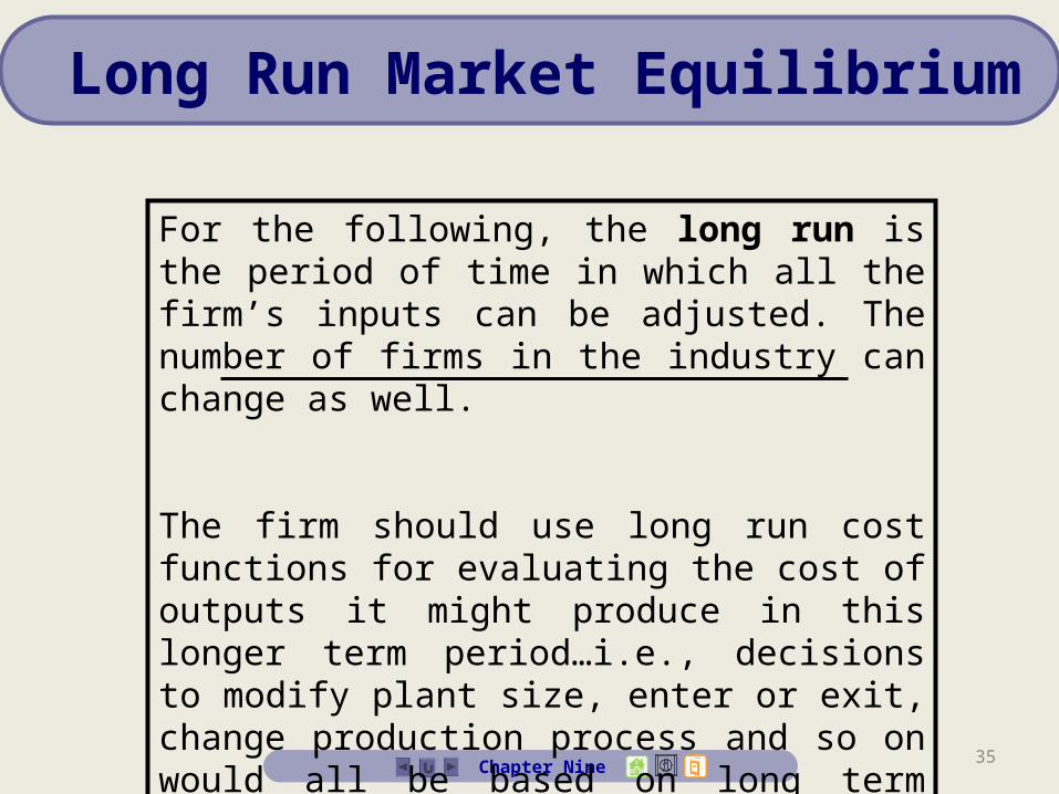
For the following, the long run is the period of time in which all the firm’s inputs can be adjusted. The number of firms in the industry can change as well.
The firm should use long run cost functions for evaluating the cost of outputs it might produce in this longer term period…i.e., decisions to modify plant size, enter or exit, change production process and so on would all be based on long term analysis

36
P
6 q
$/unit
(000 units/yr)
SMC0 SAC0
1.8
SAC1
SMC1
MC
AC
Example: Incentive to Change Plant Size
Example: Incentive to Change Plant Size
Chapter Nine
Long Run Market Equilibrium
For example, at P, this firm has an incentive to change plant size to level K1 from K0:For example, at P, this firm has an incentive to change plant size to level K1 from K0:
37Chapter Nine
Firm’s Long Run Supply Curve
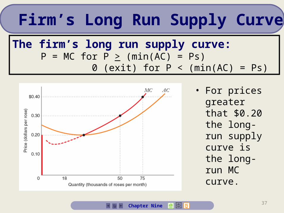
• For prices greater that $0.20 the long-run supply curve is the long-run MC curve.
The firm’s long run supply curve:P = MC for P > (min(AC) = Ps)
0 (exit) for P < (min(AC) = Ps)
38
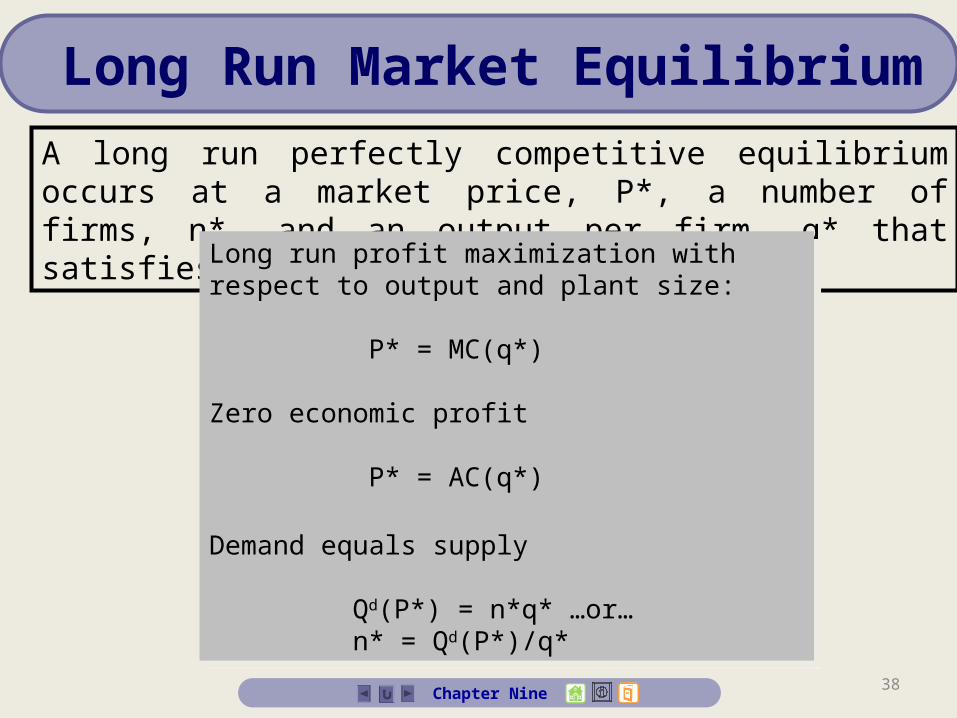
A long run perfectly competitive equilibrium occurs at a market price, P*, a number of firms, n*, and an output per firm, q* that satisfies:
Chapter Nine
Long Run Market Equilibrium
Long run profit maximization with respect to output and plant size:
P* = MC(q*)
Zero economic profit
P* = AC(q*)
Demand equals supply
Qd(P*) = n*q* …or…n* = Qd(P*)/q*
Long run profit maximization with respect to output and plant size:
P* = MC(q*)
Zero economic profit
P* = AC(q*)
Demand equals supply
Qd(P*) = n*q* …or…n* = Qd(P*)/q*
39
ACMC
SAC
SMC
P*
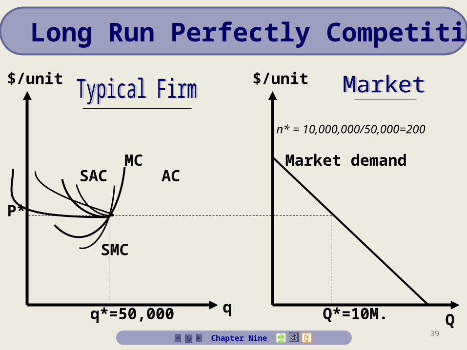
q*=50,000 qQ
$/unit$/unit
Market demand
Q*=10M.
n* = 10,000,000/50,000=200
Chapter Nine
Long Run Perfectly Competitive
40Chapter Nine
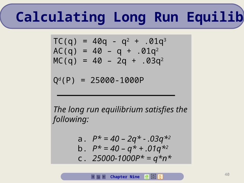
Calculating Long Run Equilibrium
TC(q) = 40q - q2 + .01q3
AC(q) = 40 – q + .01q2
MC(q) = 40 – 2q + .03q2
Qd(P) = 25000-1000P
The long run equilibrium satisfies the following:
a. P* = 40 – 2q* - .03q*2
b. P* = 40 – q* + .01q*2
c. 25000-1000P* = q*n*
TC(q) = 40q - q2 + .01q3
AC(q) = 40 – q + .01q2
MC(q) = 40 – 2q + .03q2
Qd(P) = 25000-1000P
The long run equilibrium satisfies the following:
a. P* = 40 – 2q* - .03q*2
b. P* = 40 – q* + .01q*2
c. 25000-1000P* = q*n*
41Chapter Nine
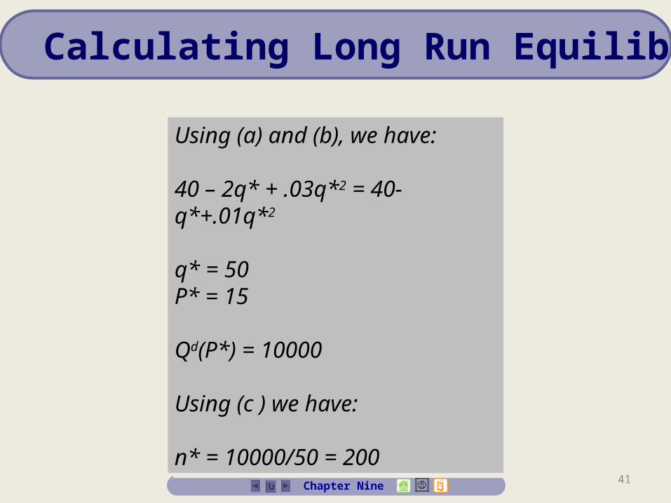
Calculating Long Run Equilibrium
Using (a) and (b), we have:
40 – 2q* + .03q*2 = 40-q*+.01q*2
q* = 50P* = 15
Qd(P*) = 10000
Using (c ) we have:
n* = 10000/50 = 200
Using (a) and (b), we have:
40 – 2q* + .03q*2 = 40-q*+.01q*2
q* = 50P* = 15
Qd(P*) = 10000
Using (c ) we have:
n* = 10000/50 = 200
42Chapter Nine
Calculating Long Run Equilibrium
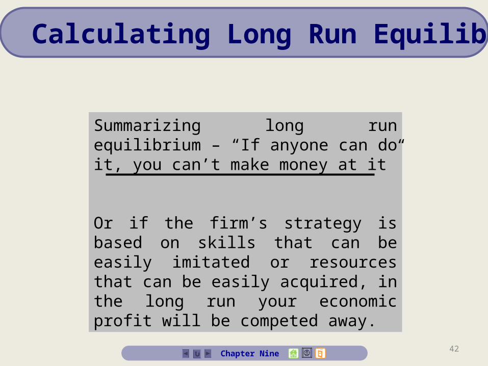
Summarizing long run equilibrium – “If anyone can do it, you can’t make money at it”
Or if the firm’s strategy is based on skills that can be easily imitated or resources that can be easily acquired, in the long run your economic profit will be competed away.
Summarizing long run equilibrium – “If anyone can do it, you can’t make money at it”
Or if the firm’s strategy is based on skills that can be easily imitated or resources that can be easily acquired, in the long run your economic profit will be competed away.
43Chapter Nine
Long Run Market Supply Curve
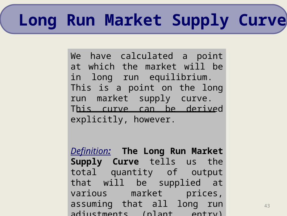
We have calculated a point at which the market will be in long run equilibrium. This is a point on the long run market supply curve. This curve can be derived explicitly, however.
Definition: The Long Run Market Supply Curve tells us the total quantity of output that will be supplied at various market prices, assuming that all long run adjustments (plant, entry) take place.
44Chapter Nine
Since new entry can occur in the long run, we cannot obtain the long run market supply curve by summing the long run supplies of current market participants
Instead, we must construct the long run market supply curve.
We reason that, in the long run, output expansion or contraction in the industry occurs along a horizontal line corresponding to the minimum level of long run average cost.
If P > min(AC), entry would occur, driving price back to min(AC)
If P < min(AC), firms would earn negative profits and would supply nothing
Long Run Market Supply Curve
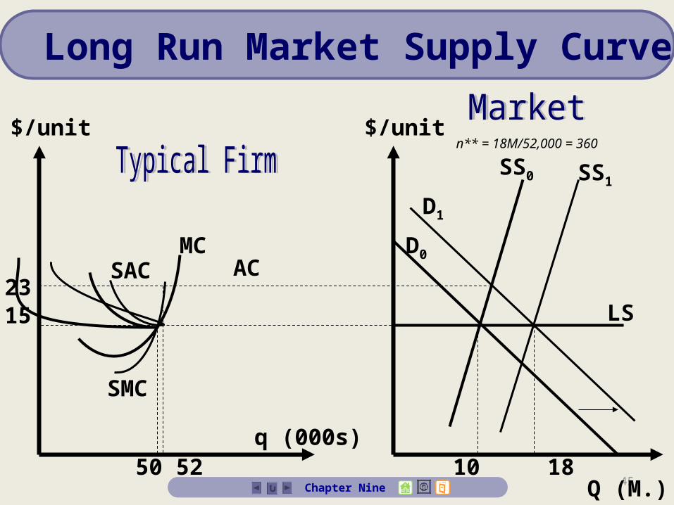
45
ACMC
SAC
SMC
15
50 52q (000s)
Q (M.)
$/unit$/unit
10 18
n** = 18M/52,000 = 360
SS0
23
D0
D1
SS1
LS
Chapter Nine
Long Run Market Supply Curve
46Chapter Nine
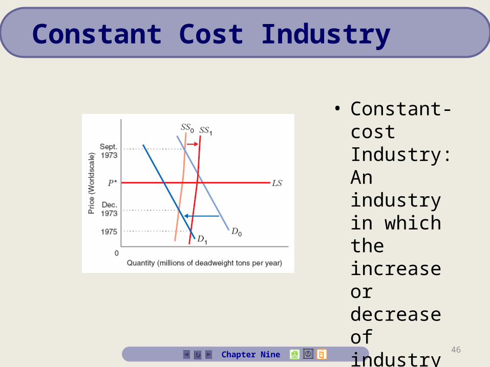
Constant Cost Industry
• Constant-cost Industry: An industry in which the increase or decrease of industry output does not affect the price of inputs.
47Chapter Nine
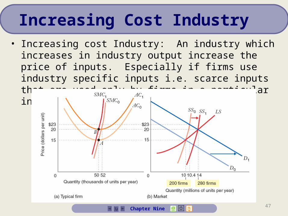
Increasing Cost Industry• Increasing cost Industry: An industry which increases in industry
output increase the price of inputs. Especially if firms use industry specific inputs i.e. scarce inputs that are used only by firms in a particular industry and no other industry.
48Chapter Nine
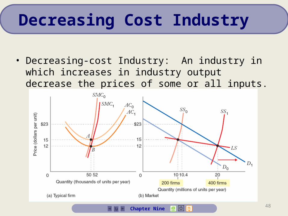
Decreasing Cost Industry
• Decreasing-cost Industry: An industry in which increases in industry output decrease the prices of some or all inputs.
49Chapter Nine
Economic Rent
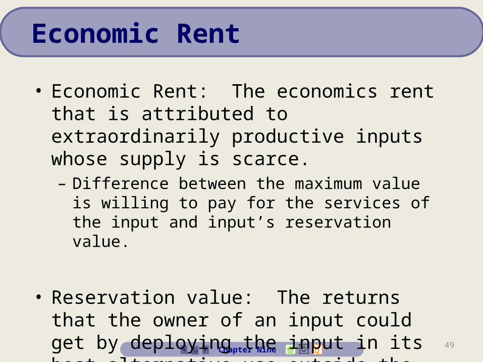
• Economic Rent: The economics rent that is attributed to extraordinarily productive inputs whose supply is scarce. – Difference between the maximum value is willing to pay
for the services of the input and input’s reservation value.
• Reservation value: The returns that the owner of an input could get by deploying the input in its best alternative use outside the industry.
50Chapter Nine
Economic Rent
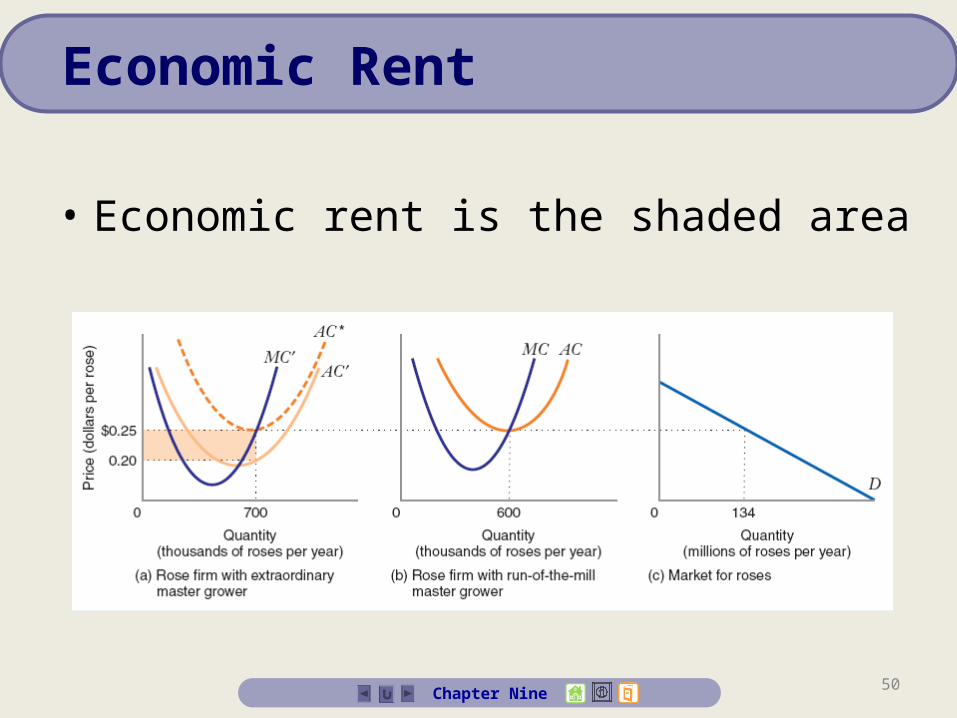
• Economic rent is the shaded area
51Chapter Nine
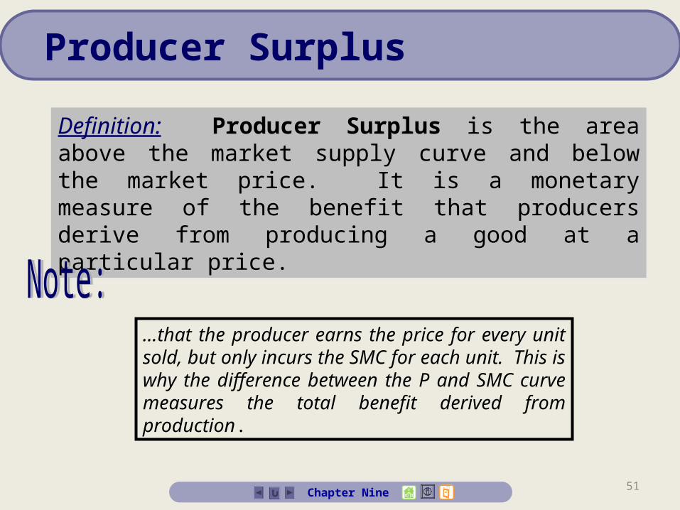
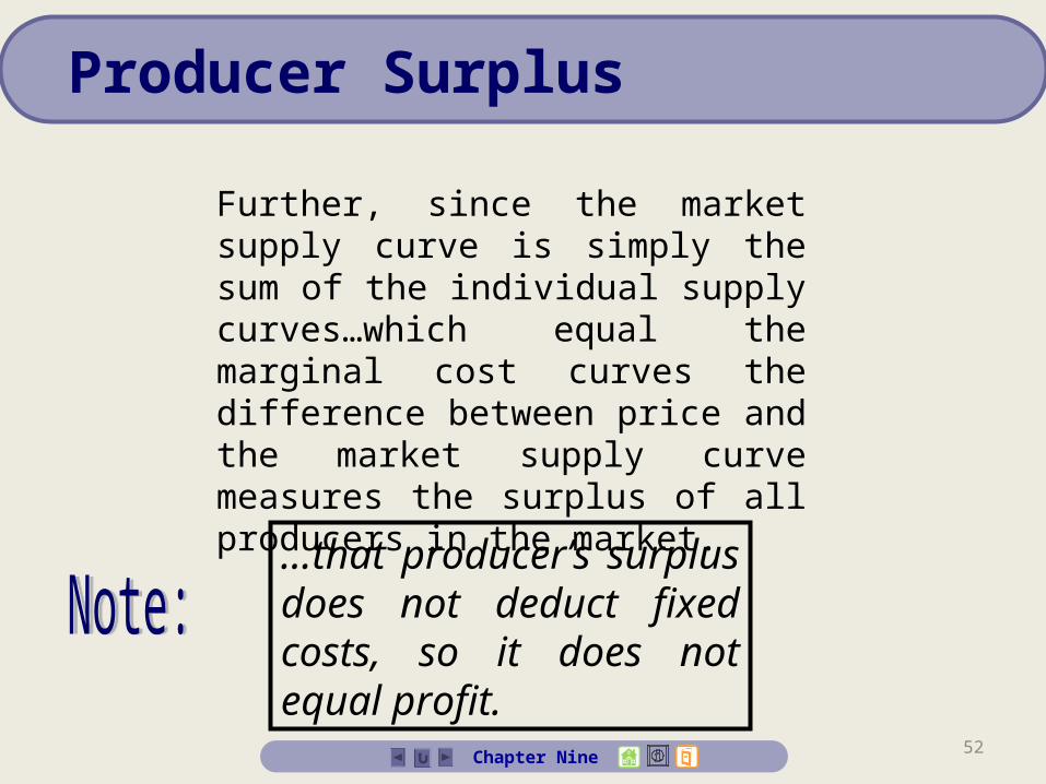
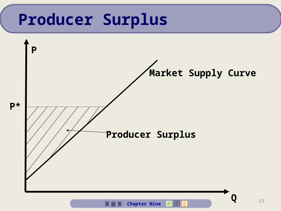
Definition: Producer Surplus is the area above the market supply curve and below the market price. It is a monetary measure of the benefit that producers derive from producing a good at a particular price.
Definition: Producer Surplus is the area above the market supply curve and below the market price. It is a monetary measure of the benefit that producers derive from producing a good at a particular price.
Producer Surplus
…that the producer earns the price for every unit sold, but only incurs the SMC for each unit. This is why the difference between the P and SMC curve measures the total benefit derived from production.
52Chapter Nine
Producer Surplus
Further, since the market supply curve is simply the sum of the individual supply curves…which equal the marginal cost curves the difference between price and the market supply curve measures the surplus of all producers in the market.
…that producer’s surplus does not deduct fixed costs, so it does not equal profit.
53Q
P
Market Supply Curve
P*
Producer Surplus
Chapter Nine
Producer Surplus
54Chapter Nine
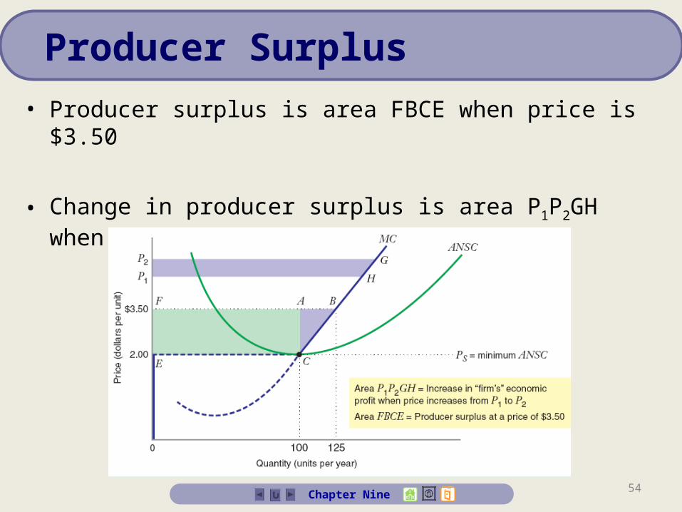
Producer Surplus• Producer surplus is area FBCE when price is $3.50
• Change in producer surplus is area P1P2GH when price moves from P1 to P2.
55Chapter Nine
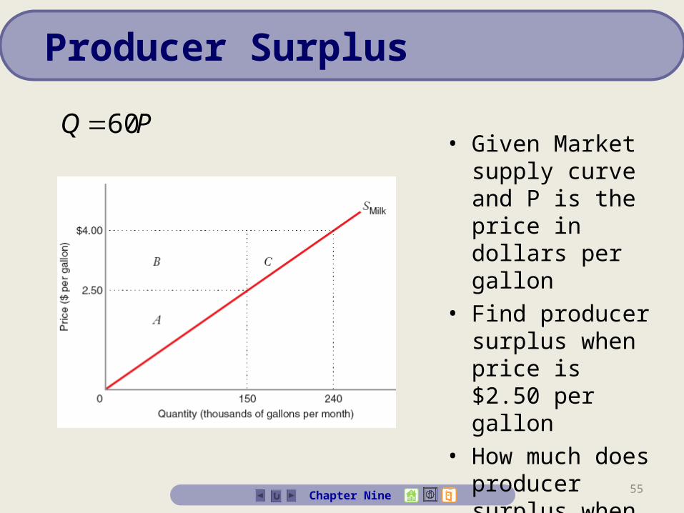
Producer Surplus
PQ 60• Given Market
supply curve and P is the price in dollars per gallon
• Find producer surplus when price is $2.50 per gallon
• How much does producer surplus when price of milk increases from $2.50 to $4.00
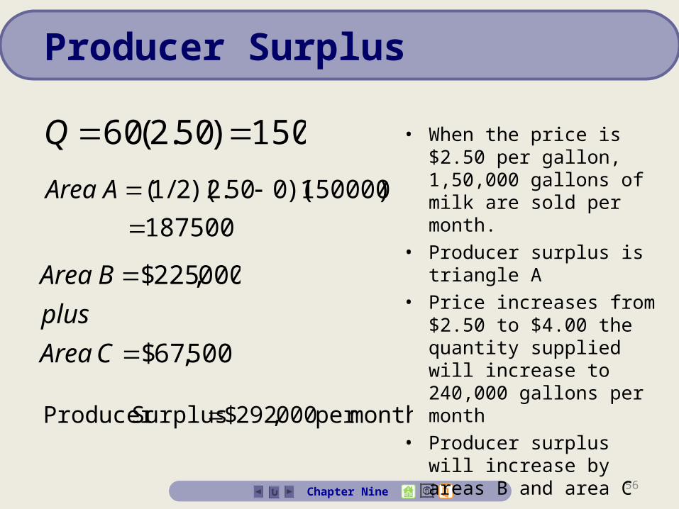
56Chapter Nine
Producer Surplus
150)50.2(60 Q
187500
)150000)(050.2)(2/1(
AArea
500,67$
000,225$
CArea
plus
BArea
monthper 000,292$ SurplusProducer
• When the price is $2.50 per gallon, 1,50,000 gallons of milk are sold per month.
• Producer surplus is triangle A• Price increases from $2.50 to
$4.00 the quantity supplied will increase to 240,000 gallons per month
• Producer surplus will increase by areas B and area C