Perceptual Organization and Recognition of Indoor Scenes from RGB-D Images

Saurabh Gupta, Pablo Arbelaez, and Jitendra MalikUniversity of California, Berkeley - Berkeley, CA 94720

{sgupta, arbelaez, malik}@eecs.berkeley.edu

Abstract

We address the problems of contour detection, bottom-up grouping and semantic segmentation using RGB-D data.We focus on the challenging setting of cluttered indoorscenes, and evaluate our approach on the recently intro-duced NYU-Depth V2 (NYUD2) dataset [27]. We proposealgorithms for object boundary detection and hierarchicalsegmentation that generalize the gPb − ucm approach of[2] by making effective use of depth information. We showthat our system can label each contour with its type (depth,normal or albedo). We also propose a generic method forlong-range amodal completion of surfaces and show its ef-fectiveness in grouping. We then turn to the problem of se-mantic segmentation and propose a simple approach thatclassifies superpixels into the 40 dominant object categoriesin NYUD2. We use both generic and class-specific featuresto encode the appearance and geometry of objects. We alsoshow how our approach can be used for scene classifica-tion, and how this contextual information in turn improvesobject recognition. In all of these tasks, we report signifi-cant improvements over the state-of-the-art.

1. IntroductionIn this paper, we study the problem of image understand-

ing in indoor scenes from color and depth data. The output

of our approach is shown in Figure 1: given a single RGB-D

image, our system produces contour detection and bottom-

up segmentation, grouping by amodal completion, and se-

mantic labeling of objects and scene surfaces.

The problem of three dimensional scene understanding

from monocular images has received considerable attention

in recent years [11, 8, 10, 20, 19, 25], and different aspects

have been explored. Some works have addressed the task

of inferring coarse 3D layout of outdoor scenes, exploiting

appearance and geometric information [11, 25]. Recently,

the focus has shifted towards the more difficult case of clut-

tered indoor scenes [10, 20, 19, 9]. In this context, the no-

tion of affordance and the functionality of objects for hu-

man use acquires importance. Thus, [10] recovers walk-

Figure 1: Output of our system: From a single color

and depth image, we produce bottom-up segmentation

(top-right), long range completion(bottom-left), semantic

segmentation (bottom-middle) and contour classification

(bottom-right).

able surfaces by reasoning on the location and shape of fur-

niture, [20, 19] reason about the 3D geometry of the room

and objects, while [9] focuses on interpreting the scene in a

human-centric perspective.

With the availability of consumer RGB-D sensors (like

the Microsoft Kinect), a new area of research has opened up

in computer vision around using 3D information for tasks

which have traditionally been very hard. A good example

is its first application for real-time human pose recognition

[26], in use in the Microsoft XBOX. Subsequently, there

have also been numerous papers in both robotics and vision

communities looking at object and instance recognition us-

ing RGB-D data [28, 17] and dense reconstruction of in-

door scenes and objects from multiple scenes. Using range

data for recognition has a long history, some examples be-

ing spin images [13] and 3D shape contexts [7]. The focus

of these works has mostly been object recognition and not

scene understanding.

More recent research which directly relates to our work

is Silberman et al. [27]. They also look at the task of

bottom-up RGB-D segmentation and semantic scene label-

ing. They modify the algorithm of [12] to use depth for

bottom-up segmentation and then look at the task of seman-

2013 IEEE Conference on Computer Vision and Pattern Recognition

1063-6919/13 $26.00 © 2013 IEEE

DOI 10.1109/CVPR.2013.79

562

2013 IEEE Conference on Computer Vision and Pattern Recognition

1063-6919/13 $26.00 © 2013 IEEE

DOI 10.1109/CVPR.2013.79

562

2013 IEEE Conference on Computer Vision and Pattern Recognition

1063-6919/13 $26.00 © 2013 IEEE

DOI 10.1109/CVPR.2013.79

564

tic segmentation using context features derived from infer-

ring support relationships in the scene. Ren et al. [23] use

features based on kernel descriptors on superpixels and its

ancestors from a region hierarchy followed by a Markov

Random Field (MRF) based context modeling. Koppula etal. [15] also study the problem of indoor scene parsing with

RGB-D data in the context of mobile robotics, where mul-

tiple views of the scene are acquired with a Kinect sensor

and subsequently merged into a full 3D reconstruction. The

3D point cloud is over-segmented and used as underlying

structure for an MRF model.

Our work differs from the references above in both our

approach to segmentation and to recognition. We visit the

segmentation problem afresh from ground-up and develop a

gPb [2] like machinery which combines depth information

naturally, giving us significantly better bottom-up segmen-

tation when compared to earlier works. We also look at the

interesting problem of amodal completion [14] and obtain

long range grouping giving us much better bottom-up re-

gion proposals. Finally, we are also able to label each edge

as being a depth edge, a normal edge, or neither.

Our approach for recognition builds on insights from the

performance of different methods on the PASCAL VOC

segmentation challenge [6]. We observe that approaches

like [4, 1], which focus on classifying bottom-up regions

candidates using strong features on the region have obtained

significantly better results than MRF-based methods [16].

We build on this motivation and propose new features to

represent bottom-up region proposals (which in our case are

non-overlapping superpixels and their amodal completion),

and use randomized decision tree forest [3, 5] and SVM

classifiers.

In addition to semantic segmentation, we look at the

problem of RGB-D scene classification and show that

knowledge of the scene category helps improve accuracy

of semantic segmentation.

This paper is organized as follows. In Sect. 2 we pro-

pose an algorithm for estimating the gravity direction from

a depth map. In Sect. 3 we describe our algorithm and re-

sults for perceptual organization. In Sect. 4 we describe our

semantic segmentation approach, and then apply our ma-

chinery to scene classification in Sect. 5.

2. Extracting a Geocentric Coordinate FrameWe note that the direction of gravity imposes a lot of

structure on how the real world looks (the floor and other

supporting surfaces are always horizontal, the walls are al-

ways vertical). Hence, to leverage this structure, we develop

a simple algorithm to determine the direction of gravity.

Note that this differs from the Manhattan World assump-

tion made by, e.g. [9] in the past. The assumption that there

are 3 principal mutually orthogonal directions is not univer-

sally valid. On the other hand the role of the gravity vector

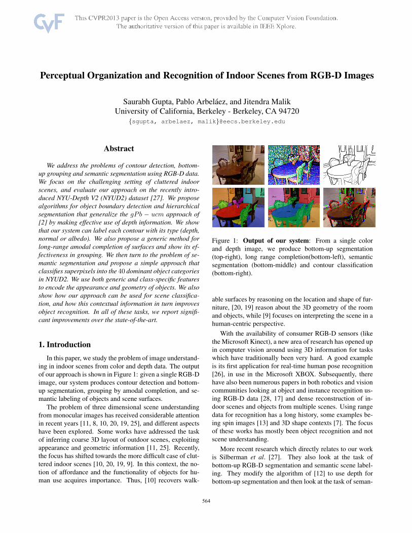
Figure 2: Cumulative

distribution of angle of

the floor with the esti-

mated gravity direction.

in architectural design is equally important for a hut in Zim-

babwe or an apartment in Manhattan.

Since we have depth data available, we propose a sim-

ple yet robust algorithm to estimate the direction of gravity.

Intuitively, the algorithm tries to find the direction which is

the most aligned to or most orthogonal to locally estimated

surface normal directions at as many points as possible. The

algorithm starts with an estimate of the gravity vector and

iteratively refines the estimate via the following 2 steps.

1. Using the current estimate of the gravity direction

gi−1, make hard-assignments of local surface normals

to aligned set N‖ and orthogonal set N⊥, (based on

a threshold d on the angle made by the local surface

normal with gi−1). Stack the vectors in N‖ to form a

matrix N‖, and similarly in N⊥ to form N⊥.

N‖ = {n : θ(n, gi−1) < d or θ(n, gi−1) > 180◦ − d}N⊥ = {n : 90◦ − d < θ(n, gi−1) < 90◦ + d}

where, θ(a, b) = Angle between a and b.

Typically, N‖ would contain normals from points on

the floor and table-tops andN⊥ would contain normals

from points on the walls.

2. Solve for a new estimate of the gravity vector gi which

is as aligned to normals in the aligned set and as or-

thogonal to the normals in the orthogonal set as pos-

sible. This corresponds to solving the following op-

timization problem, which simplifies into finding the

eigen-vector with the smallest eigen value of the 3× 3matrix, N⊥N t

⊥ −N‖N t‖.

ming:‖g‖2=1

∑

n∈N⊥

cos2(θ(n, g)) +∑

n∈N‖

sin2(θ(n, g))

Our initial estimate for the gravity vector g0 is the Y-

axis, and we run 5 iterations with d = 45◦ followed by 5

iterations with d = 15◦.To benchmark the accuracy of our gravity direction, we

use the metric of [27]. We rotate the point cloud to align the

Y-axis with the estimated gravity direction and look at the

angle the floor makes with the Y-axis. We show the cumu-

lative distribution of the angle of the floor with the Y-axis in

563563565

figure 2. Note that our gravity estimate is within 5◦ of the

actual direction for 90% of the images, and works as well

as the method of [27], while being significantly simpler.

3. Perceptual OrganizationOne of our main goals is to perform perceptual organi-

zation on RGB-D images. We would like an algorithm that

detects contours and produces a hierarchy of bottom-up seg-

mentations from which we can extract superpixels at any

granularity. We would also like a generic machinery that

can be trained to detect object boundaries, but that can also

be used to detect different types of geometric contours by

leveraging the depth information. In order to design such

a depth-aware perceptual organization system, we build on

the architecture of the gPb−ucm algorithm [2], which is a

widely used software for monocular image segmentation.

3.1. Geometric Contour Cues

In addition to color data, we have, at each image pixel, an

estimation of its 3D location in the scene and of its surface

normal orientation. We use this local geometric informa-

tion to compute three oriented contour signals at each pixel

in the image: a depth gradient DG which identifies the pres-

ence of a discontinuity in depth, a convex normal gradient

NG+ which captures if the surface bends-out at a given

point in a given direction, and a concave normal gradient

NG−, capturing if the surface bends-in.

Generalizing the color and texture gradients of gPb to

RGB-D images in not a trivial task because of the character-

istics of the data, particularly: (1) a nonlinear noise model

of the form |δZ| ∝ Z2|δd|, where δZ is the error in depth

observation, Z is the actual depth, δd is the error in dis-

parity observation (due to the triangulation-based nature of

the Kinect), causing non-stochastic and systematic quanti-

zation of the depth, (2) lack of temporal synchronization be-

tween color and depth channels, resulting in misalignment

in the dataset being used, (3) missing depth observations.

We address these issues by carefully designing geometric

contour cues that have a clear physical interpretation, using

multiple sizes for the window of analysis, not interpolating

for missing depth information, estimating normals by least

square fits to disparity instead of points in the point cloud,

and independently smoothing the orientation channels with

Savitsky-Golay [24] parabolic fitting.

In order to estimate the local geometric contour cues, we

consider a disk centered at each image location. We split the

disk into two halves at a pre-defined orientation and com-

pare the information in the two disk-halves, as suggested

originally in [22] for contour detection in monocular im-

ages. In the experiments, we consider 4 different disk radii

varying from 5 to 20 pixels and 8 orientations. We compute

the 3 local geometric gradients DG, NG+ and NG− by ex-

amining the point cloud in the 2 oriented half-disks. We first

represent the distribution of points on each half-disk with a

planar model. Then, for DG we calculate the distance be-

tween the two planes at the disk center and for NG+ and

NG− we calculate the angle between the normals of the

planes.

3.2. Contour Detection and Segmentation

We formulate contour detection as a binary pixel classi-

fication problem where the goal is to separate contour from

non-contour pixels, an approach commonly adopted in the

literature [22, 12, 2]. We learn classifiers for each orienta-

tion channel independently and combine their final outputs,

rather than training one single classifier for all contours.

Contour Locations We first consider the average of all

local contour cues in each orientation and form a combined

gradient by taking the maximum response across orienta-

tions. We then compute the watershed transform of the

combined gradient and declare all pixels on the watershed

lines as possible contour locations. Since the combined gra-

dient is constructed with contours from all the cues, the

watershed over-segmentation guarantees full recall for the

contour locations. We then separate all the candidates by

orientation.

Labels We transfer the labels from ground-truth manual

annotations to the candidate locations for each orientation

channel independently. We first identify the ground-truth

contours in a given orientation, and then declare as positives

the candidate contour pixels in the same orientation within

a distance tolerance. The remaining candidates in the same

orientation are declared negatives.

Features For each orientation, we consider as features

our geometric cues DG, NG+ and NG− at 4 scales, and

the monocular cues from gPb: BG, CG and TG at their

3 default scales. We also consider three additional cues:

the depth of the pixel, a spectral gradient [2] obtained by

globalizing the combined local gradient via spectral graph

partitioning, and the length of the oriented contour.

Oriented Contour Detectors We use as classifiers sup-

port vector machines (SVMs) with additive kernels [21],

which allow learning nonlinear decision boundaries with an

efficiency close to linear SVMs, and use their probabilistic

output as the strength of our oriented contour detectors.

Hierarchical Segmentation Finally, we use the generic

machinery of [2] to construct a hierarchy of segmentations,

by merging regions of the initial over-segmentation based

on the average strength of our oriented contour detectors.

3.3. Amodal Completion

The hierarchical segmentation obtained thus far only

groups regions which are continuous in 2D image space.

However, surfaces which are continuous in 3D space can be

fragmented into smaller pieces because of occlusion. Com-

mon examples are floors, table tops and counter tops, which

564564566

often get fragmented into small superpixels because of ob-

jects resting on them.

In monocular images, the only low-level signal that can

be used to do this long-range grouping is color and texture

continuity which is often unreliable in the presence of spa-

tially varying illumination. However, in our case with ac-

cess to 3D data, we can use the more robust and invariant

geometrical continuity to do long-range grouping. We op-

erationalize this idea as follows:

1. Estimate low dimensional parametric geometric mod-

els for individual superpixels obtained from the hierar-

chical segmentation.

2. Greedily merge superpixels into bigger more complete

regions based on the agreement among the parametric

geometric fits, and re-estimate the geometric model.

In the context of indoor scenes we use planes as our low di-

mensional geometric primitive. As a measure of the agree-

ment we use the (1) orientation (angle between normals to

planar approximation to the 2 superpixels) and (2) residual

error (symmetrized average distance between points on one

superpixel from the plane defined by the other superpixel);

and use a linear function of these 2 features to determine

which superpixels to merge.

As an output of this greedy merging, we get a set of non-

overlapping regions which consists of both long and short

range completions of the base superpixels.

3.4. Results

We train and test our oriented contour detectors using

the instance level boundary annotations of the NYUD2 as

the ground-truth labels. We train on the 795 images of the

train set and evaluate our performance on the 654 images

of the test set. In the dominant orientations (i.e. horizon-

tal and vertical), we obtain in the order of 106 data points

both for training and testing, and an order of magnitude less

candidates for the other orientations.

We evaluate performance using the standard benchmarks

of the Berkeley Segmentation Dataset [2]: Precision-Recall

on boundaries and Ground truth Covering of regions. We

consider two natural baselines for bottom-up segmentation:

the algorithm gPb − ucm, which does not have access to

depth information, and the approach of [27], made available

by the authors (noted NYUD2 baseline), which produces a

small set (5) of nested segmentations using color and depth.

Figure 3 and Table 1 1 present the results. Our depth-

aware segmentation system produces contours of far higher

quality than gPb − ucm, improving the Average Precision

1ODS refers to optimal dataset scale, OIS refers to optimal image scale,

bestC is the average overlap of the best segment in the segmentation hierar-

chy to each ground truth region. We refer the reader to [2] for more details

about these metrics.

Figure 3: BoundaryBenchmark onNYUD2: Our

approach (red)

significantly out-

performs baselines

[2](black) and

[27](blue).

(AP) from 0.55 to 0.70 and the maximal F-measure (ODS

in Table 1 - left) from 0.62 to 0.69. In terms of region

quality, the improvement is also significant, increasing the

best ground truth covering of a single level in the hierarchy

(ODS in Table 1 - right) from 0.55 to 0.62, and the qual-

ity of the best segments across the hierarchy from 0.69 to

0.75. Thus, on average, for each ground truth object mask

in the image, there is one region in the hierarchy that over-

laps 75% with it. The comparison against the NYUD2 base-

line, which has access to depth information, is also largely

favorable for our approach. In all the benchmarks, the per-

formance of the NYUD2 baseline lies between gPb− ucmand our algorithm.

In [27], only the coarsest level of the NYUD2 base-

line is used as spatial support to instantiate a probabilistic

model for semantic segmentation. However, a drawback of

choosing one single level of superpixels in later applications

is that it inevitably leads to over- or under-segmentation.

Table 2 compares in detail this design choice against our

amodal completion approach. A first observation is that our

base superpixels are finer than the NYUD2 ones: we ob-

tain a larger number and our ground truth covering is lower

(from 0.61 to 0.56), indicating higher over-segmentation in

our superpixels. The boundary benchmark confirms this

observation, as our F-measure is slightly lower, but with

higher Recall and lower Precision.

The last row of Table 2 provides empirical support for

our amodal completion strategy: by augmenting our fine su-

perpixels with a small set of amodally completed regions (6

on average), we preserve the boundary Recall of the under-

lying over-segmentation while improving the quality of the

regions significantly, increasing the bestC score from 0.56to 0.63. The significance of this jump can be judged by

comparison with the ODS score of the full hierarchy (Table

1 - right), which is 0.62: no single level in the full hierarchy

would produce better regions than our amodally completed

superpixels.

Our use of our depth-aware contour cues DG, NG+,

and NG−, is further justified because it allows us to also

565565567

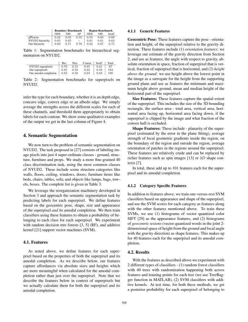
Boundary Benchmark Region BenchmarkODS OIS AP ODS OIS bestC

gPb-ucm 0.62 0.65 0.55 0.55 0.60 0.69NYUD2 hierarchy 0.65 0.65 − 0.61 0.61 0.63Our hierarchy 0.69 0.71 0.70 0.62 0.67 0.75

Table 1: Segmentation benchmarks for hierarchical seg-

mentation on NYUD2.

Rec Prec F-meas bestC Total

NYUD2 superpixels 0.78 0.55 0.65 0.61 87Our superpixels 0.85 0.50 0.63 0.56 184Our amodal completion 0.85 0.50 0.63 0.63 190

Table 2: Segmentation benchmarks for superpixels on

NYUD2.

infer the type for each boundary, whether it is an depth edge,

concave edge, convex edge or an albedo edge. We simply

average the strengths across the different scales for each of

these channels, and threshold them appropriately to obtain

labels for each contour. We show some qualitative examples

of the output we get in the last column of Figure 4.

4. Semantic Segmentation

We now turn to the problem of semantic segmentation on

NYUD2. The task proposed in [27] consists of labeling im-

age pixels into just 4 super-ordinate classes - ground, struc-

ture, furniture and props. We study a more fine-grained 40

class discrimination task, using the most common classes

of NYUD2. These include scene structure categories like

walls, floors, ceiling, windows, doors; furniture items like

beds, chairs, tables, sofa; and objects like lamps, bags, tow-

els, boxes. The complete list is given in Table 3.

We leverage the reorganization machinery developed in

Section 3 and approach the semantic segmentation task by

predicting labels for each superpixel. We define features

based on the geocentric pose, shape, size and appearance

of the superpixel and its amodal completion. We then train

classifiers using these features to obtain a probability of be-

longing to each class for each superpixel. We experiment

with random decision tree forests [3, 5] (RF), and additive

kernel [21] support vector machines (SVM).

4.1. Features

As noted above, we define features for each super-

pixel based on the properties of both the superpixel and its

amodal completion. As we describe below, our features

capture affordances via absolute sizes and heights which

are more meaningful when calculated for the amodal com-

pletion rather than just over the superpixel. Note that we

describe the features below in context of superpixels but

we actually calculate them for both the superpixel and its

amodal completion.

4.1.1 Generic Features

Geocentric Pose: These features capture the pose - orienta-

tion and height, of the superpixel relative to the gravity di-

rection. These features include (1) orientation features: we

leverage our estimate of the gravity direction from Section

2, and use as features, the angle with respect to gravity, ab-

solute orientation in space, fraction of superpixel that is ver-

tical, fraction of superpixel that is horizontal, and (2) heightabove the ground: we use height above the lowest point in

the image as a surrogate for the height from the supporting

ground plane and use as features the minimum and maxi-

mum height above ground, mean and median height of the

horizontal part of the superpixel.

Size Features: These features capture the spatial extent

of the superpixel. This includes the size of the 3D bounding

rectangle, the surface area - total area, vertical area, hori-

zontal area facing up, horizontal area facing down, if the

superpixel is clipped by the image and what fraction of the

convex hull is occluded.

Shape Features: These include - planarity of the super-

pixel (estimated by the error in the plane fitting), average

strength of local geometric gradients inside the region, on

the boundary of the region and outside the region, average

orientation of patches in the regions around the superpixel.

These features are relatively crude and can be replaced by

richer features such as spin images [13] or 3D shape con-

texts [7].

In total, these add up to 101 features each for the super-

pixel and its amodal completion.

4.1.2 Category Specific Features

In addition to features above, we train one-versus-rest SVM

classifiers based on appearance and shape of the superpixel,

and use the SVM scores for each category as features along

with the other features mentioned above. To train these

SVMs, we use (1) histograms of vector quantized color

SIFT [29] as the appearance features, and (2) histograms

of geocentric textons (vector quantized words in the joint 2-

dimensional space of height from the ground and local angle

with the gravity direction) as shape features. This makes up

for 40 features each for the superpixel and its amodal com-

pletion.

4.2. Results

With the features as described above we experiment with

2 different types of classifiers - (1) random forest classifiers

with 40 trees with randomization happening both across

features and training points for each tree (we use TreeBag-

ger function in MATLAB), (2) SVM classifiers with addi-

tive kernels. At test time, for both these methods, we get

a posterior probability for each superpixel of belonging to

566566568

each of the 40 classes and assign the most probable class to

each superpixel.

We use the standard split of NYUD2 with 795 training

set images and 654 test set images for evaluation. To pre-

vent over-fitting because of retraining on the same set, we

train our category specific SVMs only on half of the train

set.

Performance on the 40 category task We measure the

performance of our algorithm using the Jaccard index (true

predictions divided by union of predictions and true labels -

same as the metric used for evaluation in the PASCAL VOC

segmentation task) between the predicted pixels and ground

truth pixels for each category. As an aggregate measure, we

look at the frequency weighted average of the class-wise

Jaccard index.

We report the performance in Table 3 (first 4 rows in the

two tables). As baselines, we use [27]-Structure Classifier,

where we retrain their structure classifiers for the 40 class

task, and [23], where we again retrained their model for

this task on this dataset using code available on their web-

site2. We observe that we are able to do well on scene sur-

faces (walls, floors, ceilings, cabinets, counters), and most

furniture items (bed, chairs, sofa). We do poorly on small

objects, due to limited training data and weak shape fea-

tures (our features are designed to describe big scene level

surfaces and objects). We also consistently outperform the

baselines. Fig. 4 presents some qualitative examples, more

are provided in the supplemental material.

Ablation Studies In order to gain insights into how

much each type of feature contributes towards the semantic

segmentation task, we conduct an ablation study by remov-

ing parts from the final system. We report our observations

in Table 4. Randomized decision forests (RF) work slightly

better than SVMs when using only generic or category spe-

cific features, but SVMs are able to more effectively com-

bine information when using both these sets of features. Us-

ing features from amodal completion also provides some

improvement. [27]-SP: we also retrain our system on the

superpixels from [27] and obtain better performance than

[27] (36.51) indicating that the gain in performance comes

in from better features and not just from better bottom-up

segmentation. [23] features: we also tried the RGB-D ker-

nel descriptor features from [23] on our superpixels, and

observe that they do slightly worse than our category spe-

cific features.

Performance on NYUD2 4 category task We compare

our performance with existing results on the super-ordinate

category task as defined in[27] in Table 5. To generate pre-

dictions for the super-ordinate categories, we simply retrain

our classifiers to predict the 4 super-ordinate category la-

bels. As before we report the pixel wise Jaccard index for

2We run their code on NYUD2 with our bottom-up segmentation hier-

archy using the same classifier hyper-parameters as specified in their code.

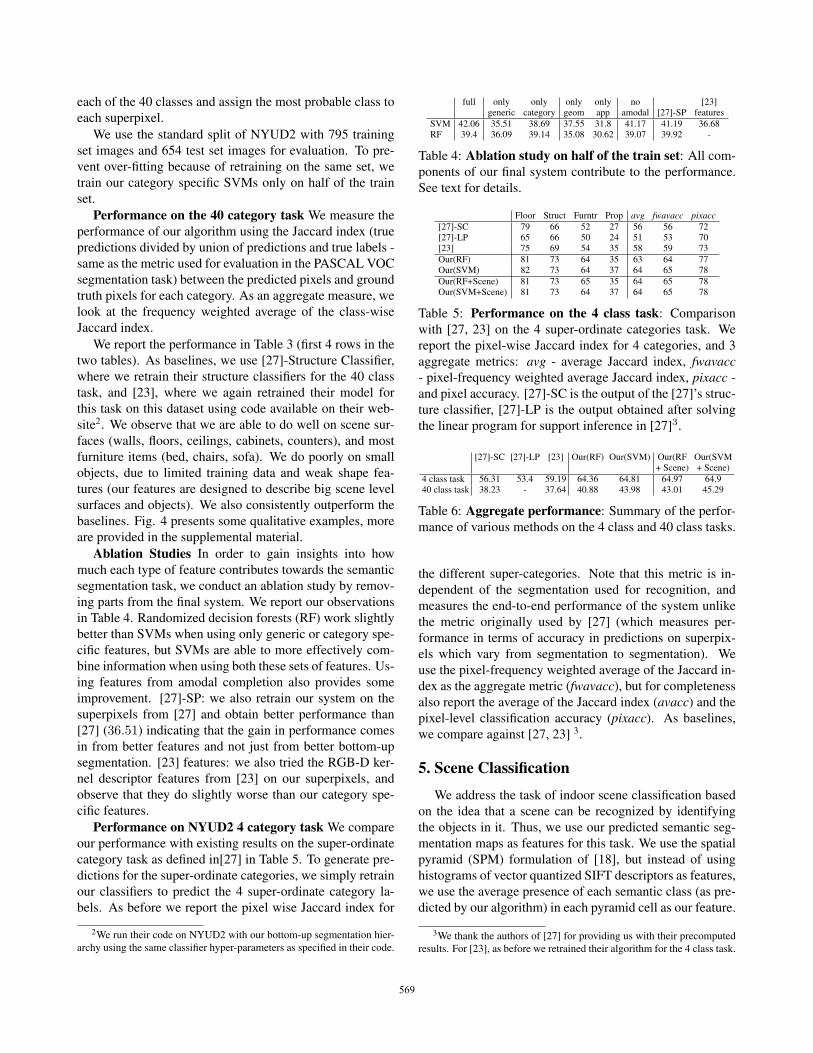
full only only only only no [23]generic category geom app amodal [27]-SP features

SVM 42.06 35.51 38.69 37.55 31.8 41.17 41.19 36.68RF 39.4 36.09 39.14 35.08 30.62 39.07 39.92 -

Table 4: Ablation study on half of the train set: All com-

ponents of our final system contribute to the performance.

See text for details.

Floor Struct Furntr Prop avg fwavacc pixacc[27]-SC 79 66 52 27 56 56 72[27]-LP 65 66 50 24 51 53 70[23] 75 69 54 35 58 59 73

Our(RF) 81 73 64 35 63 64 77Our(SVM) 82 73 64 37 64 65 78

Our(RF+Scene) 81 73 65 35 64 65 78Our(SVM+Scene) 81 73 64 37 64 65 78

Table 5: Performance on the 4 class task: Comparison

with [27, 23] on the 4 super-ordinate categories task. We

report the pixel-wise Jaccard index for 4 categories, and 3

aggregate metrics: avg - average Jaccard index, fwavacc- pixel-frequency weighted average Jaccard index, pixacc -

and pixel accuracy. [27]-SC is the output of the [27]’s struc-

ture classifier, [27]-LP is the output obtained after solving

the linear program for support inference in [27]3.

[27]-SC [27]-LP [23] Our(RF) Our(SVM) Our(RF Our(SVM+ Scene) + Scene)

4 class task 56.31 53.4 59.19 64.36 64.81 64.97 64.940 class task 38.23 - 37.64 40.88 43.98 43.01 45.29

Table 6: Aggregate performance: Summary of the perfor-

mance of various methods on the 4 class and 40 class tasks.

the different super-categories. Note that this metric is in-

dependent of the segmentation used for recognition, and

measures the end-to-end performance of the system unlike

the metric originally used by [27] (which measures per-

formance in terms of accuracy in predictions on superpix-

els which vary from segmentation to segmentation). We

use the pixel-frequency weighted average of the Jaccard in-

dex as the aggregate metric (fwavacc), but for completeness

also report the average of the Jaccard index (avacc) and the

pixel-level classification accuracy (pixacc). As baselines,

we compare against [27, 23] 3.

5. Scene Classification

We address the task of indoor scene classification based

on the idea that a scene can be recognized by identifying

the objects in it. Thus, we use our predicted semantic seg-

mentation maps as features for this task. We use the spatial

pyramid (SPM) formulation of [18], but instead of using

histograms of vector quantized SIFT descriptors as features,

we use the average presence of each semantic class (as pre-

dicted by our algorithm) in each pyramid cell as our feature.

3We thank the authors of [27] for providing us with their precomputed

results. For [23], as before we retrained their algorithm for the 4 class task.

567567569

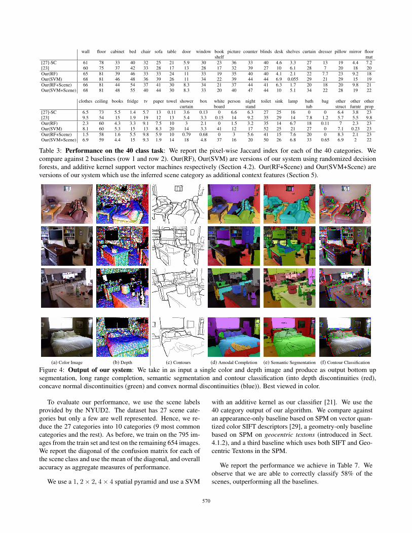
wall floor cabinet bed chair sofa table door window book picture counter blinds desk shelves curtain dresser pillow mirror floorshelf mat

[27]-SC 61 78 33 40 32 25 21 5.9 30 23 36 33 40 4.6 3.3 27 13 19 4.4 7.2[23] 60 75 37 42 33 28 17 13 28 17 32 39 27 10 6.1 28 7 20 18 20

Our(RF) 65 81 39 46 33 33 24 11 33 19 35 40 40 4.1 2.1 22 7.7 23 9.2 18Our(SVM) 68 81 46 48 36 39 26 11 34 22 39 44 44 6.9 0.055 29 21 29 15 19

Our(RF+Scene) 66 81 44 54 37 41 30 8.3 34 21 37 44 41 6.3 1.7 20 18 20 9.8 21Our(SVM+Scene) 68 81 48 55 40 44 30 8.3 33 20 40 47 44 10 5.1 34 22 28 19 22

clothes ceiling books fridge tv paper towel shower box white person night toilet sink lamp bath bag other other othercurtain board stand tub struct furntr prop

[27]-SC 6.5 73 5.5 1.4 5.7 13 0.11 3.6 0.13 0 6.6 6.3 27 25 16 0 0 6.4 3.8 23[23] 9.5 54 15 1.9 19 12 13 5.4 3.3 0.15 14 9.2 35 29 14 7.8 1.2 5.7 5.5 9.8

Our(RF) 2.3 60 4.3 3.3 9.1 7.5 10 3 2.1 0 1.5 3.2 35 14 6.7 18 0.11 7 2.3 23Our(SVM) 8.1 60 5.3 15 13 8.3 20 14 3.3 41 12 17 52 25 21 27 0 7.1 0.23 23

Our(RF+Scene) 1.5 58 1.6 5.5 9.8 5.9 10 0.79 0.68 0 3 5.6 41 15 7.6 20 0 8.3 2.1 23Our(SVM+Scene) 6.9 59 4.4 15 9.3 1.9 14 18 4.8 37 16 20 50 26 6.8 33 0.65 6.9 2 22

Table 3: Performance on the 40 class task: We report the pixel-wise Jaccard index for each of the 40 categories. We

compare against 2 baselines (row 1 and row 2). Our(RF), Our(SVM) are versions of our system using randomized decision

forests, and additive kernel support vector machines respectively (Section 4.2). Our(RF+Scene) and Our(SVM+Scene) are

versions of our system which use the inferred scene category as additional context features (Section 5).

(a) Color Image (b) Depth (c) Contours (d) Amodal Completion (e) Semantic Segmentation (f) Contour Classification

Figure 4: Output of our system: We take in as input a single color and depth image and produce as output bottom up

segmentation, long range completion, semantic segmentation and contour classification (into depth discontinuities (red),

concave normal discontinuities (green) and convex normal discontinuities (blue)). Best viewed in color.

To evaluate our performance, we use the scene labels

provided by the NYUD2. The dataset has 27 scene cate-

gories but only a few are well represented. Hence, we re-

duce the 27 categories into 10 categories (9 most common

categories and the rest). As before, we train on the 795 im-

ages from the train set and test on the remaining 654 images.

We report the diagonal of the confusion matrix for each of

the scene class and use the mean of the diagonal, and overall

accuracy as aggregate measures of performance.

We use a 1, 2× 2, 4× 4 spatial pyramid and use a SVM

with an additive kernel as our classifier [21]. We use the

40 category output of our algorithm. We compare against

an appearance-only baseline based on SPM on vector quan-

tized color SIFT descriptors [29], a geometry-only baseline

based on SPM on geocentric textons (introduced in Sect.

4.1.2), and a third baseline which uses both SIFT and Geo-

centric Textons in the SPM.

We report the performance we achieve in Table 7. We

observe that we are able to correctly classify 58% of the

scenes, outperforming all the baselines.

568568570

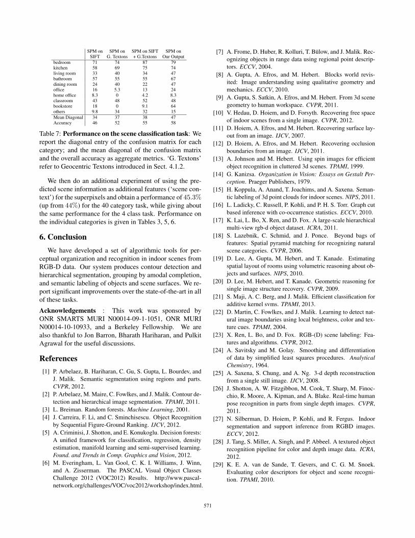
SPM on SPM on SPM on SIFT SPM onSIFT G. Textons + G.Textons Our Output

bedroom 71 74 87 79kitchen 58 69 75 74living room 33 40 34 47bathroom 57 55 55 67dining room 24 40 22 47office 16 5.3 13 24home office 8.3 0 4.2 8.3classroom 43 48 52 48bookstore 18 0 9.1 64others 9.8 34 32 15

Mean Diagonal 34 37 38 47Accuracy 46 52 55 58

Table 7: Performance on the scene classification task: We

report the diagonal entry of the confusion matrix for each

category; and the mean diagonal of the confusion matrix

and the overall accuracy as aggregate metrics. ‘G. Textons’

refer to Geocentric Textons introduced in Sect. 4.1.2.

We then do an additional experiment of using the pre-

dicted scene information as additional features (‘scene con-

text’) for the superpixels and obtain a performance of 45.3%(up from 44%) for the 40 category task, while giving about

the same performance for the 4 class task. Performance on

the individual categories is given in Tables 3, 5, 6.

6. ConclusionWe have developed a set of algorithmic tools for per-

ceptual organization and recognition in indoor scenes from

RGB-D data. Our system produces contour detection and

hierarchical segmentation, grouping by amodal completion,

and semantic labeling of objects and scene surfaces. We re-

port significant improvements over the state-of-the-art in all

of these tasks.

Acknowledgements : This work was sponsored by

ONR SMARTS MURI N00014-09-1-1051, ONR MURI

N00014-10-10933, and a Berkeley Fellowship. We are

also thankful to Jon Barron, Bharath Hariharan, and Pulkit

Agrawal for the useful discussions.

References[1] P. Arbelaez, B. Hariharan, C. Gu, S. Gupta, L. Bourdev, and

J. Malik. Semantic segmentation using regions and parts.

CVPR, 2012.

[2] P. Arbelaez, M. Maire, C. Fowlkes, and J. Malik. Contour de-

tection and hierarchical image segmentation. TPAMI, 2011.

[3] L. Breiman. Random forests. Machine Learning, 2001.

[4] J. Carreira, F. Li, and C. Sminchisescu. Object Recognition

by Sequential Figure-Ground Ranking. IJCV, 2012.

[5] A. Criminisi, J. Shotton, and E. Konukoglu. Decision forests:

A unified framework for classification, regression, density

estimation, manifold learning and semi-supervised learning.

Found. and Trends in Comp. Graphics and Vision, 2012.

[6] M. Everingham, L. Van Gool, C. K. I. Williams, J. Winn,

and A. Zisserman. The PASCAL Visual Object Classes

Challenge 2012 (VOC2012) Results. http://www.pascal-

network.org/challenges/VOC/voc2012/workshop/index.html.

[7] A. Frome, D. Huber, R. Kolluri, T. Bulow, and J. Malik. Rec-

ognizing objects in range data using regional point descrip-

tors. ECCV, 2004.

[8] A. Gupta, A. Efros, and M. Hebert. Blocks world revis-

ited: Image understanding using qualitative geometry and

mechanics. ECCV, 2010.

[9] A. Gupta, S. Satkin, A. Efros, and M. Hebert. From 3d scene

geometry to human workspace. CVPR, 2011.

[10] V. Hedau, D. Hoiem, and D. Forsyth. Recovering free space

of indoor scenes from a single image. CVPR, 2012.

[11] D. Hoiem, A. Efros, and M. Hebert. Recovering surface lay-

out from an image. IJCV, 2007.

[12] D. Hoiem, A. Efros, and M. Hebert. Recovering occlusion

boundaries from an image. IJCV, 2011.

[13] A. Johnson and M. Hebert. Using spin images for efficient

object recognition in cluttered 3d scenes. TPAMI, 1999.

[14] G. Kanizsa. Organization in Vision: Essays on Gestalt Per-ception. Praeger Publishers, 1979.

[15] H. Koppula, A. Anand, T. Joachims, and A. Saxena. Seman-

tic labeling of 3d point clouds for indoor scenes. NIPS, 2011.

[16] L. Ladicky, C. Russell, P. Kohli, and P. H. S. Torr. Graph cut

based inference with co-occurrence statistics. ECCV, 2010.

[17] K. Lai, L. Bo, X. Ren, and D. Fox. A large-scale hierarchical

multi-view rgb-d object dataset. ICRA, 2011.

[18] S. Lazebnik, C. Schmid, and J. Ponce. Beyond bags of

features: Spatial pyramid matching for recognizing natural

scene categories. CVPR, 2006.

[19] D. Lee, A. Gupta, M. Hebert, and T. Kanade. Estimating

spatial layout of rooms using volumetric reasoning about ob-

jects and surfaces. NIPS, 2010.

[20] D. Lee, M. Hebert, and T. Kanade. Geometric reasoning for

single image structure recovery. CVPR, 2009.

[21] S. Maji, A. C. Berg, and J. Malik. Efficient classification for

additive kernel svms. TPAMI, 2013.

[22] D. Martin, C. Fowlkes, and J. Malik. Learning to detect nat-

ural image boundaries using local brightness, color and tex-

ture cues. TPAMI, 2004.

[23] X. Ren, L. Bo, and D. Fox. RGB-(D) scene labeling: Fea-

tures and algorithms. CVPR, 2012.

[24] A. Savitsky and M. Golay. Smoothing and differentiation

of data by simplified least squares procedures. AnalyticalChemistry, 1964.

[25] A. Saxena, S. Chung, and A. Ng. 3-d depth reconstruction

from a single still image. IJCV, 2008.

[26] J. Shotton, A. W. Fitzgibbon, M. Cook, T. Sharp, M. Finoc-

chio, R. Moore, A. Kipman, and A. Blake. Real-time human

pose recognition in parts from single depth images. CVPR,

2011.

[27] N. Silberman, D. Hoiem, P. Kohli, and R. Fergus. Indoor

segmentation and support inference from RGBD images.

ECCV, 2012.

[28] J. Tang, S. Miller, A. Singh, and P. Abbeel. A textured object

recognition pipeline for color and depth image data. ICRA,

2012.

[29] K. E. A. van de Sande, T. Gevers, and C. G. M. Snoek.

Evaluating color descriptors for object and scene recogni-

tion. TPAMI, 2010.

569569571