Perception vs. Reality: The Relationship between Low … · lower-income households actually...
27
Page 1 of 27 Perception vs. Reality: The Relationship between Low-Income Homeownership, Perceived Financial Stress, and Financial Hardship Kim Manturuk 1 , Sarah Riley 1 , and Janneke Ratcliffe 1 Corresponding author: Kim Manturuk 919.843.5441 [email protected] 1 UNC Center for Community Capital 1700 Martin Luther King Blvd, CB# 3452, Suite 129 Chapel Hill, NC 27517
Transcript of Perception vs. Reality: The Relationship between Low … · lower-income households actually...
Page 1 of 27
Perception vs. Reality: The Relationship between Low-Income Homeownership, Perceived Financial Stress, and Financial Hardship
Kim Manturuk1, Sarah Riley1, and Janneke Ratcliffe1
Corresponding author: Kim Manturuk 919.843.5441
1 UNC Center for Community Capital 1700 Martin Luther King Blvd, CB# 3452, Suite 129
Chapel Hill, NC 27517
Page 2 of 27
ABSTRACT
This research examines how homeowners and renters were impacted by the financial crisis
in 2009. We build from the hypothesis that homeownership provides people a sense of stability
and control which decreases the extent to which they feel psychologically stressed as a result of
financial hardship. Our study tests whether owning a home affected either the degree to which
lower-income households actually experienced financial hardship or the extent to which they
perceived they were financially stressed. Using a unique data source - a survey of a sample of
lower-income borrowers who obtained affordable mortgages to buy homes through the
Community Advantage Program (CAP) and a comparison panel of renters – we collected data in
2009 on the effects of, and responses to, the financial crisis. From a portfolio performance
standpoint, CAP loans have performed relatively well. Our analysis of the survey data finds that,
although both renters and owners experienced similar levels of financial hardship, the
homeowners were less psychologically stressed overall and reported feeling more satisfied with
their financial situation.

Page 3 of 27
Introduction
Although the recent boom and bust in the housing markets has made it controversial,
homeownership has been considered a keystone of opportunity in the US economic system and a
central element of social policy since the 1930’s. Particularly from the mid-1990’s through the
mid-2000’s, advocates and policy makers sought to expand homeownership among segments of
the population whose homeownership rates lagged, namely minority and lower-income
households, by combating discriminatory lending practices and encouraging the extension of
credit with more flexible underwriting rules.
But, as has become painfully clear, there is a big difference between making more good
mortgages possible and making as many mortgages as possible. During the sub-prime mortgage
boom of 2003 - 2007, flexibility was carried to extremes, extending mortgage credit under terms
and conditions that were unsustainable and feeding a house price bubble that would inevitably
burst. In its wake, these lending excesses left a foreclosure crisis, a credit crunch, a global
recession, double-digit job losses, and the loss of a staggering $7 trillion in housing wealth.1
This is a watershed opportunity for researchers and policy makers to re-examine the value of
homeownership, especially for low- to moderate-income households who often have fewer other
assets to draw on and whose long-term financial outlook is more vulnerable to shocks. While
there is no shortage of opinions on this issue, there is a lack of real-time data. However, the
Center for Community Capital at the University of North Carolina at Chapel Hill can offer a
unique data source for the analysis of this question. Over the past 10 years, the Center has
researched mortgage loans made to low-and-moderate income (LMI) borrowers through a
groundbreaking partnership referred to as “The Community Advantage Program” (CAP). From
1999 to 2009, CAP funded nearly 50,000 home mortgages nationwide. This unique portfolio can

Page 4 of 27
provide important evidence as to the benefits and pitfalls of homeownership for a population
traditionally underserved by the mainstream market, particularly as the timing of their
homeownership experience encompasses both housing boom and bust episodes.
CAP Loan Performance
From a portfolio performance standpoint, CAP loans have performed relatively well
considering prevailing conditions. As of the end of 2009, most borrowers had still experienced
strong overall equity gains--the median CAP owner realized appreciation of $20,459. This
represented two-thirds of her annual income, and earned her more than she would have earned
following the Dow Jones Industrial Average, but just below what she would have earned putting
the same total amount in a CD over the same period. However, considering her low initial equity
investment, she has generated a double digit annual rate of return -- more than 30% per annum.
This success is largely due to the fact that these low income and minority borrowers were
qualified for and obtained affordable, 30-year, fixed rate, amortizing mortgages, underwritten for
ability to repay (Quercia, Ding, Ratcliffe).
This is not to say that all is smooth sailing, however. Since inception, 4% of the loans have
been foreclosed upon, and another 14% of the borrowers have, at some point in their mortgage
history, been 60-or-more days delinquent. Although the rate of serious delinquency has been less
than half the delinquency rate of subprime loans, the economic crisis has put a strain on many of
the CAP households. For example, nearly one third of the owners said their economic situation
had gotten worse between 2008 and 2009 versus only about a quarter who reported an
improvement, and some borrowers have negative equity, particularly those who bought late in
the cycle.
Research Objectives

Page 5 of 27
Survey data from the CAP study allows us to look beyond these top-line indicators to better
understand the complex interaction between homeownership status, economic conditions,
individual behavior, and psychological well-being. For the last eight years we have conducted in-
depth interviews with a panel of homeowners and a comparison panel of renters, roughly
matched by location and income. Beginning in 2009, survey questions focused on the effects of
and responses to the financial crisis.
We aim to answer the following questions: Has there has been an increase in stress
(financial or general stress) since the recession began? If so, what are the triggers? Overall, how
satisfied are homeowners and renters with their financial situation during the economic crisis?
Our analysis finds that although both renters and owners are experiencing similar levels of
financial stress, the LMI owners were less stressed overall and reported significantly higher
financial satisfaction, even after controlling for a range of factors. These findings suggest a
beneficial effect from owning one’s own home.
Theory
What evidence do we have to determine whether or not extending homeownership to
underserved households is beneficial? As a wealth-building mechanism, housing represents a
greater share of the wealth of lower-income households than for higher income households
(Bucks et al, 2009). Therefore, the continuing fall in the stock of US housing equity threatens to
wipe out the wealth of families whose assets are most concentrated in their homes. Moreover,
appreciation has a negative effect on affordability. In 2008, among working households earning
50-80% of area median income, 32% of owners paid more than 50% of their income toward
housing costs, while only 7% of renters paid this much (Waldrip, 2009).

Page 6 of 27
A syntheses of the research on the costs and benefits of homeownership for low income
and minority households suggests that overall, the financial benefits are as likely to be realized
by low-income and minority households as by others But this finding comes with the caveat
that less well-resourced households have a more tenuous hold on homeownership. They
conclude that the wealth building potential of homeownership actually realized is sensitive to a
number of factors: length of time spent in homeownership versus renting, level of rents relative
to home prices, house price changes, timing, location, and financing among them (Herbert and
Belsky 2006).
Thus, homeownership may not always build financial security for low-income
households. To estimate the relative wealth-building effects of homeownership, Bostic and Lee
(2009) simulated the wealth accumulation effects for low-income owner and renter households
for 72 combinations of household type, mortgage instrument, neighborhood, appreciation rates,
and time horizons. In most scenarios, homeowners come out ahead. However, in some scenarios
renting was actually a better outcome financially speaking, particularly when low-income
households purchase homes in middle-income neighborhoods and low-appreciation markets with
down payments of 5% or less. However, as the authors point out, their simulations rely on
stylized assumptions about household behavior and do not necessarily reflect actual outcomes.
The literature also raises concern over labor-related immobility (McCarthy, Van Zandt and Rohe,
2002) and a lock-in effect (Haurin and Rosenthal, 2004) of homeownership for those with less
equity, higher transaction costs on lower-balance loans, and fewer economic options.
The literature on the social and psychological benefits of homeownership for lower
income households is less developed but nevertheless suggests a number of social and
psychological benefits. Low-income owners generally report more satisfaction with homes and

Page 7 of 27
neighborhoods than renters, and nearly the same levels as owners overall (Herbert and Belsky
2006). Studies of low-income owners and renters in Baltimore by Rohe and Stegman (1994) and
Rohe and Basolo (1997) found mixed evidence of psychological impacts of homeownership; it
had no effect on homeowners’ perceived control over life 3 years after buying though it was
correlated with improved self-esteem indirectly as a result of better housing conditions, and was
strongly associated with increased overall satisfaction with life.
Moreover, we are only beginning to examine homeowner reaction to the financial crisis.
In a recent National Housing Survey, Fannie Mae (2010) found three in eight respondents from a
national sample including owners and renters stressed about their ability to pay debts, with a
much greater share of renters (46%) than owners (25%) somewhat or very stressed. Sixty one
percent of 2010 respondents felt the economy was on the wrong track, compared to just 43% in
2003. Interestingly, renters were less pessimistic than owners, with 11% of renters versus 23% of
owners, respectively, projecting a deterioration in their family’s financial situation. Still, there
was strong agreement that owning a home makes financial sense because of potential rent
increases for renters and home value appreciation even among delinquent borrowers (85%) and
underwater borrowers (75%). Over half (55%) of owners say they were sacrificing financially
some or a great deal to own their homes, yet 94% of owners said that homeownership has been a
positive experience, including an astonishing 82% of delinquent borrowers and 91% of
underwater borrowers. Meanwhile, 79% of renters reported that renting has been positive, which
is less than the share of delinquent or underwater owners who reported a positive experience
with ownership. More than half the general population agreed that a high rate of homeownership
is very important for the strength of their local community, and only 16% said that it is not

Page 8 of 27
important. Even 76% of renters described community homeownership as somewhat or very
important.
Though some of these seemingly conflicting responses may stem from the fact that the
decision to buy a home is largely driven by non-financial factors, the responses convey quite
mixed messages among all kinds of households (Fannie Mae 2010). However, the connection
between economic outcomes of homeownership and psychological experiences is not so clear.
There is a lack of research examining the linkages between tenure, economic conditions and
psychological stress, particularly among low-income households.
Data
The CAP program aims to shed light on the benefits and pitfalls of financing
homeownership for lower-income and minority households. The program was launched in 1998,
when the Ford Foundation made a $50 million grant to Self-Help, a North Carolina-based CDFI.
Based on its own successful track record of making mortgages to underserved households in
North Carolina and with the help of the Ford funding to serve as credit enhancement, Self-Help
convinced Fannie Mae to buy mortgages originated under CRA and affordable housing programs
that did not qualify for purchase into the mainstream secondary market, provided Self-Help
indemnified Fannie Mae from default losses. Self-Help purchases such mortgages from banks
around the country and delivers them to Fannie Mae, while the original lenders retain servicing
responsibilities.
Insert Table 1 about here
Since its inception, CAP has funded 46,000 mortgages for more than $4 billion. The
median borrower’s income is $30,800 and the median mortgage, $79,000. Table 1 provides
descriptive data on the CAP profile. While the lenders custom designed their own programs to

Page 9 of 27
meet market needs, all of the programs combined features that reduced cash required to close and
allowed for flexible ways to verify repayment ability and creditworthiness. Certainly all would
be considered quite risky by today’s standards: more than two-thirds of the loans had original
loan to value in excess of 95%, and almost half of the borrowers had original credit scores of 660
or less or no score at all. These programs successfully targeted underserved markets: the median
borrower earned 60% of the median income for the area in which they lived, and a
disproportionate share of the borrowers were minorities (39%) and single female-headed
households (40%).
The Community Advantage Panel Survey
The Center for Community Capital maintains origination data on all of the CAP loans
and tracks a sample of approximately 3000 CAP borrowers. To analyze comparatively the effects
of homeownership, we also follow and administer parallel annual surveys to a panel of low-
income renters, roughly matched by geographic location to the owners2. In previous studies, we
have found that many of the borrowers have improved their housing picture by exercising their
option to refinance into even lower-cost loans (Spader and Quercia, 2009), while those who
moved up experienced even bigger appreciation gains than those who remained in their original
CAP-funded properties (Riley, Freeman and Quercia, 2010). Our research has detected non-
financial benefits as well. The CAP homeowners are more likely than renters to vote in local
elections (Manturuk, Lindblad, and Quercia 2009) and participate in neighborhood organizations
(Manturuk, Lindblad, and Quercia 2010).
Yet most of these findings predate the recent foreclosure crisis, property value declines,
and job losses. How is the current economic situation affecting homeowners’ financial
conditions and behaviors? We have found that default rates are low among CAP borrowers:

Page 10 of 27
fewer than 5% of the nearly 50,000 homeowners have been foreclosed on. On the other hand, we
know that although the median CAP owner has maintained substantial equity gains well into the
recession, a minority appear to be in a negative equity situation, particularly those purchasing
late in the cycle and in more distressed markets. But what effects are the economic conditions
having on the attitudes of the households?
Methods and Limitations
This study uses CAP data to examine lower-income homeownership in the context of the
recent housing crisis. We use the panel survey data of owners and renters who responded to both
the 2008 and 2009 surveys. The analysis uses variables from the 2008 survey to predict general
stress, financial stress, and financial satisfaction in 2009. We begin with 2,216 owners and 797
renters and use coarsened exact matching to extrapolate a small well-matched sample of
homeowners and renters.
Comparing Owners to Renters
The comparison panel of renters was originally drawn with the intent of matching the
owner panel as closely as possible in terms of geography and income. Still, the profile of the
renter panel differs somewhat from that of the owners. For example, the renter panel participants
tend to have lower incomes and are less likely to be married than the homeowners. As a result,
descriptive comparisons between the two groups can be misleading, and any comparative
analysis requires using statistical controls to adjust for underlying socio-economic differences
Generalizability
Riley, Ru, and Quercia (2009) compared the CAP survey participants with low-income
and minority respondents in the May 2003 Current Population Survey (CPS), a survey of
approximately 50,000 households designed to represent the non-institutionalized civilian

Page 11 of 27
population in the United States. They find that CAP survey participants are similar to
comparable CPS respondents with respect to household size, income distribution, and minority
representation. However, compared with CPS respondents, CAP survey participants tend to be
slightly more educated, demonstrate greater attachment to the workforce, and be much more
likely to live in the South.
We focus on three key impacts: psychological stress, financial hardship, and overall
satisfaction with financial situation. For each outcome, we tested whether owning a home in
2008, as opposed to renting, increased or decreased the impact of the recession in 2009.
Descriptive statistics for all variables are shown in Table 2. We used coarsened exact matching,
described below, to address selection bias and further strengthen the causal nature of these
analyses.
Insert Table 2 about here
Measures
There are three dependent variables, all of which were measured in 2009. First, we
measured the respondents’ overall stress levels. If homeownership provides lower-income
households with a sense of security and control which helps them weather difficult economic
times, then homeowners in our sample would have lower levels of stress than renters. If
homeownership is a burden for these families, however, then homeowners may report feeling
more stress and less control over their lives during the recession.
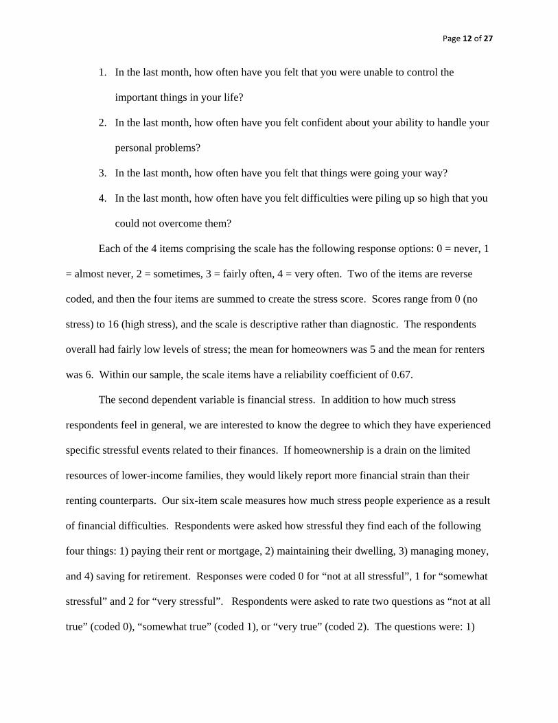
We measured overall stress using the 4-item Perceived Stress Scale (PSS) (Cohen,
Kamarck, and Mermelstein 1983). The PSS measures “the degree to which respondents found
their lives unpredictable, uncontrollable, and overloading” (Cohen and Williamson 1988). The
PSS consists of the following four questions:
Page 12 of 27
1. In the last month, how often have you felt that you were unable to control the
important things in your life?
2. In the last month, how often have you felt confident about your ability to handle your
personal problems?
3. In the last month, how often have you felt that things were going your way?
4. In the last month, how often have you felt difficulties were piling up so high that you
could not overcome them?
Each of the 4 items comprising the scale has the following response options: 0 = never, 1
= almost never, 2 = sometimes, 3 = fairly often, 4 = very often. Two of the items are reverse
coded, and then the four items are summed to create the stress score. Scores range from 0 (no
stress) to 16 (high stress), and the scale is descriptive rather than diagnostic. The respondents
overall had fairly low levels of stress; the mean for homeowners was 5 and the mean for renters
was 6. Within our sample, the scale items have a reliability coefficient of 0.67.
The second dependent variable is financial stress. In addition to how much stress
respondents feel in general, we are interested to know the degree to which they have experienced
specific stressful events related to their finances. If homeownership is a drain on the limited
resources of lower-income families, they would likely report more financial strain than their
renting counterparts. Our six-item scale measures how much stress people experience as a result
of financial difficulties. Respondents were asked how stressful they find each of the following
four things: 1) paying their rent or mortgage, 2) maintaining their dwelling, 3) managing money,
and 4) saving for retirement. Responses were coded 0 for “not at all stressful”, 1 for “somewhat
stressful” and 2 for “very stressful”. Respondents were asked to rate two questions as “not at all
true” (coded 0), “somewhat true” (coded 1), or “very true” (coded 2). The questions were: 1)

Page 13 of 27
How true is it that you pay too much rent or mortgage? and 2) How true is it that you have too
much debt? The responses to these six items were summed to create an index of financial stress.
The Cronbach’s alpha for the scale is 0.75.
The final dependent variable is a more general measure of satisfaction with one’s
financial situation. It is possible that homeownership could prompt people to feel more satisfied
with their finances, even if they are financially stressed, because they are satisfied with their
decision to become a homeowner. Alternatively, homeowners may feel less satisfied because it
would be more difficult for them to relocate in response to a job loss or other unexpected
financial hardship, or because their housing investment is eroding. We measured financial
satisfaction using a single-item question. Respondents were simply asked, “How satisfied are
you with your overall financial situation?” There were three response options: very satisfied,
somewhat satisfied, and not at all satisfied. The majority of respondents, 52% of renters and
60% of homeowners, were “somewhat satisfied”. The responses were coded one through three
and modeled using an ordinal regression model.
Method
For this study, we use coarsened exact matching to draw a matched sample of
homeowners and renters from our original sample. Coarsened exact matching aims to address
the selection bias that is inherent in observational studies. There are two primary flaws in
traditional regression analysis. First, the selection variable is specified by these models as
exogenous but is actually endogenous (Guo and Fraser 2009). In this research, for example, a
traditional covariate control model would model homeownership as exogenous when it is not. In
order to derive robust estimates, selection needs to be explicitly modeled (Heckman 1979, p.
153; Heckman 1978, p. 931). Second, traditional regression models assume that selection is

Page 14 of 27
independent from the outcome of interest. When this assumption is violated, as it often is,
regression models yield biased and inconsistent estimation of the regression coefficients (Berk
2004 ; Imbens 2004, p. 4; Rosenbaum and Rubin 1983, p. 41). In the present study, respondents
selected whether to purchase a home or rent a home, and this selection must be modeled in order
to obtain unbiased results.
We use coarsened exact matching to address selection bias and reduce model dependence
(Ho et al. 2007). We first “coarsen” the independent variables which are theoretically associated
with homeownership by collapsing them in to meaningful bins. For example, we take the
continuous variable representing years of education and coarsen it to bins representing a high
school degree or less, a college degree, and an advanced degree. Second, the coarsened exact
matching algorithm creates one stratum for each unique set of covariates predicting treatment
and assigns each observation to a stratum. Strata without both a treatment and a control
observation are dropped, and the remaining observations constitute the matched sample.
Coarsened exact matching offers several advantages over other matching methods. First,
unlike most matching algorithms, coarsened exact matching allows the researcher to specify the
maximum imbalance ex ante. This produces a marked reduction in the imbalance between
treatment and control groups and, in turn, reduces selection bias and model dependence
(Blackwell et al. 2009). Another advantage of coarsened exact matching is that, unlike
propensity score-based matching, reducing the imbalance on one variable has no effect on the
other variables in the selection model. Furthermore, we are able to compare the multivariable
imbalance statistic before and after matching to determine how effective the matching is in
reducing imbalance. For this analysis, we used the Stata routine /cem/ to create the matched
Page 15 of 27
sample of homeowners and renters and then ran linear and logistic regression models to calculate
the sample average treatment effect on the treated (the homeowners).
Insert Table 3 about here
Table 3 shows the imbalance before matching between the sample of homeowners and
the sample of renters on key demographic variables. The L1 statistic indicates the level of
imbalance for each variable, and the table also shows mean difference at each quartile. The
overall multivariable imbalance is 0.94. When using coarsened exact matching, there is a trade-
off between the number of variables in the matching algorithm and the extent to which the
variables must be coarsened in order to yield a balanced sample with sufficient observations for
causal inference. The more variables that are included, and the more bins allocated per variable,
the smaller the sample size and the more imbalance will remain. The variables we included in
the matching algorithm provided a satisfactory reduction in imbalance while still covering the
key demographic differences between the homeowners and renters.
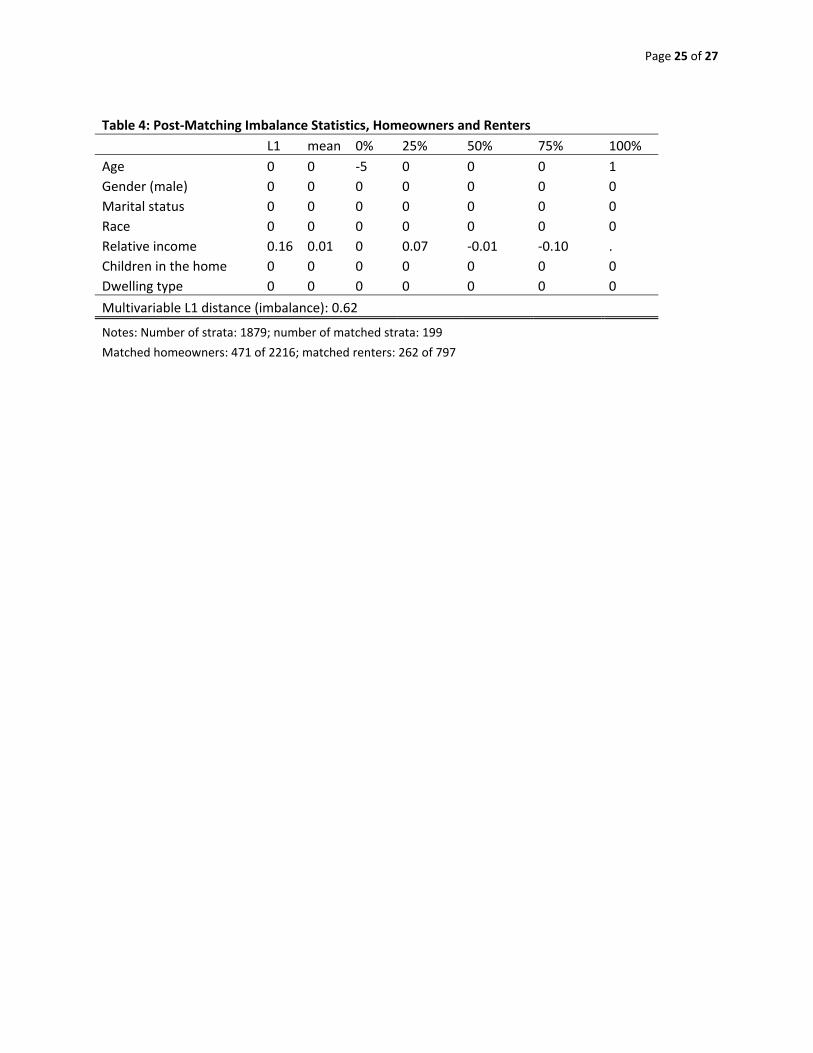
Insert Table 4 about here
Table 4 shows the imbalance statistics after matching. As shown, the multivariable
imbalance of the matched sample is 0.62, a reduction of 0.32. The /cem/ algorithm divided the
sample in to a total of 1,879 strata, 199 of which contained both a homeowners and a renter.
This resulted in a matched sample of 471 homeowners and 262 renters. Table 4 also shows that
the L1 imbalance for all the variables except relative income has been eliminated. Because the
sample is still imbalanced on relative income, the subsequent parametric models will control for
that variable.
Results
Page 16 of 27
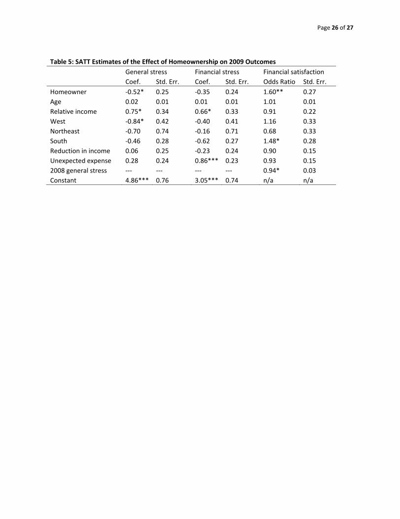
Table 5 shows coefficients from the regression models predicting general stress, financial
stress, and financial satisfaction in 2009. The first column shows the OLS coefficients for the
variables predicting general stress. Homeownership is associated with a 0.52 point reduction in
general stress. The model also indicates that people with higher relative incomes have more
stress, while those living in the west have less stress then people in other parts of the country.
Insert Table 5 about here
The second model in Table 5 indicates that homeownership is not significantly related to
financial stress. While homeownership did not give people a financial advantage during the
crisis, it also did not appear to put them at a disadvantage compared to renters. Somewhat
surprisingly, people with a higher relative income were more likely to report higher levels of
financial stress. This may be because households with higher incomes have more access to
credit and therefore more opportunities to accumulate debt. As expected, people who had
experienced an unexpected expense were more likely to feel financially stressed than those who
had not.
Finally, the last model finds a positive relationship between homeownership and financial
satisfaction. The homeowners in the CAP sample were 60% more likely to report a higher level
of satisfaction with their financial situation than the renters. Interestingly, neither of the financial
trigger event variables were associated with financial satisfaction, nor was income. We did find
a regional effect; people living in the south were significantly more likely to feel satisfied with
their financial situation, likely due to regional economic conditions. More than half the
respondents lived in17 southern states, but only two of those -- North Carolina and Oklahoma --
represent more than 4% of either sample, whereas Ohio dominates the Midwestern subset and
California and Arizona are the lead states in the Western subset. California and Arizona both saw
Page 17 of 27
substantial increases in property value from 2000 to 2006, and have since seen 30% price
declines, while the two big states in the south have both logged property value gains since 20063.
The share of mortgages 90-days past due and in foreclosure in the second quarter of 2010 in
California and Arizona is about double the level, and Ohio about 150%, of that in North Carolina
and Oklahoma, indicating more distress in those markets.4 Oklahoma logged the lowest April
2010 unemployment rate (6%) and California, the highest.5
The above analysis provides some intriguing insights. Though homeowners in our sample
were neither more nor less likely than renters to experience financial stressors during the
economic crunch, homeowners exhibited a greater perception of being in control and
significantly higher financial satisfaction than renters, suggesting that the condition of
homeownership somehow provide a greater sense of financial security.
Discussion
From the literature, macro indicators, and the CAP research as a whole, we have evidence
that suggests homeownership can be a fairly reliable contributor to wealth building for low
income households. It is also clear that the extent to which it leads to greater wealth is dependent
on a variety of factors outside of the owners’ control such as house price appreciation and
employment. The varied experiences of our CAP owners show that entering homeownership is
just a first step, and the path has lots of divergences.
Homeownership appears to ameliorate general stressors and increase financial
satisfaction, things that are related to an overall sense of life control. However, its effect on
financial stress specifically is mixed, which partly explains why people continue to debate the
issue of whether homeownership makes sense for LMI households.

Page 18 of 27
Our analysis focused on the relationships between financial stress, general stress, and
homeownership. The findings point to a cleavage between financial stress and both general
stress and financial satisfaction, at least among the homeowners in this study. We found that the
homeowners and renters both experienced financial stress to a remarkably similar degree.
Homeownership did not lesson the impacts of the financial crisis, but it also did not put people at
a financial disadvantage compared to renters. Yet, in spite of the fact that everyone experienced
similar financial stressors, the homeowners experienced less overall stress than the renters. This
suggests to us that homeownership may give people a sense of being in control of their lives,
which in turn reduces the stress they feel as a result of financial hardships. We found a similar
result when looking at how satisfied respondents were with their overall financial situation. In
spite of the fact that both groups had similar financial situations, the homeowners were again
more likely to report that they felt satisfied with their situation. This supports the idea that
owning a home gives people a sense of satisfaction or accomplishment which translates in to
feeling more satisfied.
Our analysis of stress and financial satisfaction among low income renters and owners
finds no differences for financial stress across tenure groups. We can in part explain the lack of
an obvious effect of homeownership on financial stress by observing that external conditions
moderate whether the household finds homeownership more of a financial liberator or a financial
constraint.
One important limitation, as Dietz and Haurin (2003) identify as an econometric
challenge in assessing the impacts of tenure on social and financial outcomes of interest, is that
homeowners differ in both observable and unobservable ways from renters. Thus, assessing the
effect of tenure requires consideration of underlying differences. The coarsened exact matching

Page 19 of 27
enabled us to address observable differences between the owner and renter samples, but these
groups could still be systematically different in unobserved ways.
Finally, we note again the dissonance between actual financial experiences and reports of
financial satisfaction and sense of control. The fact that low income owners experienced similar
set backs over the course of 2008 to 2009 to low-income renters, yet reported significantly lower
levels of financial and general stress, indicate that the benefits to homeownership go beyond
those that are financial, tangible and easy to measure. Ongoing research on the CAP participants
will attempt to tease these out further.
Page 20 of 27
REFERENCES
Berk, R. 2004. Regression Analysis: A Constructive Critique . Thousand Oaks, CA: Sage. Blackwell, Matthew, Stefano Iacus, Gary King, and Giuseppe Porro. 2009. cem: Coarsened
Exact Matching in Stata, The Stata Journal 9: 524--546. Bostic, Raphael W. and Kwan Ok Lee. Homeownership: America’s Dream? Insufficient Funds:
Savings, Assets, Credit and Banking Among Low-Income Households, Rebecca M. Blank and Michael S. Barr, Editors. Russell Sage Foundation.2009. NY, NY.
Bucks, Brian K., Arthur B. Kennickell, Traci L. Mach and Kevin B. Moore, 2009. Changes in
US Family Finances from 2004-2007: Evidence from the Survey of Consumer Finances. Federal Reserve Bulletin vol. 95 (February 2009), pp. A1-A55. http://www.federalreserve.gov/pubs/bulletin/2009/pdf/scf09.pdf
Dietz, Robert D. and Donald R. Haurin. 2003. The Social and Private Micro-Level
Consequences of Homeownership. Journal of Urban Economics 54: 401-450.
Cohen, S., Kamarck, T. & Mermelstein, R. 1983. “A Global Measure of Perceived Stress”, Journal of Health and Social Behavior, 24, 385-396.
Cohen, S. & Williamson, G. 1988. “Perceived Stress in a Probability Sample of the United States:, in S. Spacapan & S. Oskamp (Eds.) The Social Psychology of Health: Claremont Symposium on Applied Social Psychology, Newbury Park, CA: Sage.
Fannie Mae National Housing Survey, 2010. http://www.fanniemae.com/media/pdf/2010/National-Housing-Survey-040610.pdf.
Guo, Shenyang and Mark Fraser. 2009. Propensity Score Analysis, California: Sage Publications.
Haurin, Donald R. and Stuart S. Rosenthal, The Sustainability of Homeownership: Factors affecting the duration of homeownership and rental spells, Abt Associate, HUD PD&R, December 2004).
Heckman, James J. . 1978. "Dummy Endogenous Variables in a Simultaneous Equation
System." Econometrica 46 (4):931-959. ———. 1979. "Sample Selection Bias as a Specification Error." Econometrica 47 (1):153-161.
Herbert, Christopher E. and Eric S. Belsky, 2006. The Homeownership Experience of Low-Income and Minority Families. A Review and Synthesis of the Literature. Prepared for

Page 21 of 27
US Department of Housing and Urban Development, Office of Policy Development and Research. Abt Associates, Cambridge MA. February 2006.
Hirano, Keisuke, Guido W. Imbens, and Geert Ridder. 2003. “Efficient Estimation of Average Treatment Effects Using the Estimated Propensity Score”, Econometrica, 71:1161-1189
Imbens, Guido W. 2004. "Nonparametric Estimation of Average Treatment Effects Under
Exogeneity: A Review." The Review of Economics and Statistics 86 (1):4-29. McCarthy, George, Shannon Van Zandt and William Rohe. 2002. The Economic Benefits and
Costs of Homeownership: A Critical Assessment of the Research; Research Institute for Housing America, Working Paper No 01-02.)
Manturuk, Kim, Mark Lindblad, and Roberto Quercia. 2010. “Friends and Neighbors: Homeownership as
a Source of Social Capital”, Journal of Urban Affairs (forthcoming). Manturuk, Kim, Mark Lindblad, and Roberto Quercia. 2009. “Homeownership and Local Voting in
Disadvantaged Urban Neighborhoods”, Cityscape, 11:105-122. Quercia, Roberto G., Lei Ding, Wei Li and Janneke Ratcliffe. Risky Borrowers and Risky
Mortgages: Disaggregating Effects Using Propensity Score Matching. UNC Center for Community Capital. November 2009.
Riley, Sarah, HongYu Ru, and Roberto Quercia. 2009. The Community Advantage Program
Database: Overview and Comparison with the Current Population. Survey. Cityscape 11(3): 247-255.
Riley, Sarah, HongYu Ru, Mark Lindblad, and Roberto Quercia. 2010. Community Advantage
Panel Survey: Data Collection Update and Analysis of Panel Attrition. University of North Carolina Center for Community Capital.
Rosenbaum, Paul R. 1987. “Model-Based Direct Adjustment”, Journal of the American Statistical Association, 82:387-394.
Rosenbaum, Paul R., and Donald B. Rubin . 1983. "The Central Role of the Propensity Score in Observational Studies for Causal Effects." Biometrika 70 (1):41-55.
Spader, Jonathon and Roberto G. Quercia. May 2009. The Refinancing Transition: Equity
Extraction, Income Constraints, and Subprime Refinancing Among CRA Mortgage Borrowers, UNC Center for Community Capital (working paper).
Waldrip, Keith. Housing Affordability Trends for Working Households, Center for Housing
Policy, December 2009. http://www.nhc.org/pdf/Housing%20Affordability%20Trends.pdf)

Page 22 of 27
TABLES Table 1: Profile of CAP Funded Loans as of December, 2009 Number of Loans 46,532 Total Funding $4,060,551,059 Median Annual Income $30,792 Median Loan Amount $79,000 Median Annual Income as % of MSA Median 60% % female headed household 40.52% % Minority 39.34% % credit score 660 or less (including no score) 46.07% % LTV over 95% at origination 69.29% % with debt to income ratio 38% or lower 90.54%

Page 23 of 27
Table 2: Stress Measures: Descriptive Statistics Variable (n=3103) Freq. Mean Std. Dev. Min MaxGeneral stress 2008 5.42 2.99 0 16General stress 2009 5.53 2.92 0 16Financial stress 3.64 2.76 0 12Financial satisfaction 1.74 0.60 1 3Homeowner 2216 0 1Renter 797 0 1Relative income 0.81 0.55 0 4.19Age 41 11.41 19 92Married 1534 0 1Cohabiting 212 0 1Widowed 101 0 1Divorced 554 0 1Separated 82 0 1Single 619 0 1White 1814 0 1Black 746 0 1Hispanic 422 0 1Other race 104 0 1Children in home 1841 0 1Reduction in income 1065 0 1Unexpected expense 1318 0 1Single family dwelling 2413 0 1Apartment 499 0 1Condo/townhouse 286 0 1Other residence 160 0 1Male 1379 0 1West 292 0 1Midwest 836 0 1Northeast 84 0 1South 1891 0 1

Page 24 of 27
Table 3: Pre‐Matching Imbalance Statistics, Homeowners and Renters L1 mean 0% 25% 50% 75% 100% Age 0.20 ‐3.56 1 ‐1 ‐4 ‐7 9 Gender (male) 0.16 0.16 0 0 0 0 0 Marital status 0.35 ‐0.97 0 0 ‐2 ‐2 0 Race 0.15 ‐0.15 0 0 0 0 0 Relative income 0.42 0.46 0.00 0.35 0.42 0.58 1.17 Children in the home 0.17 0.39 0 0 1 0 2 Dwelling type 0.19 ‐0.19 0 0 0 ‐1 0
Multivariable L1 distance (imbalance): 0.94
Page 25 of 27
Table 4: Post‐Matching Imbalance Statistics, Homeowners and Renters L1 mean 0% 25% 50% 75% 100% Age 0 0 ‐5 0 0 0 1 Gender (male) 0 0 0 0 0 0 0 Marital status 0 0 0 0 0 0 0 Race 0 0 0 0 0 0 0 Relative income 0.16 0.01 0 0.07 ‐0.01 ‐0.10 . Children in the home 0 0 0 0 0 0 0 Dwelling type 0 0 0 0 0 0 0
Multivariable L1 distance (imbalance): 0.62
Notes: Number of strata: 1879; number of matched strata: 199
Matched homeowners: 471 of 2216; matched renters: 262 of 797
Page 26 of 27
Table 5: SATT Estimates of the Effect of Homeownership on 2009 Outcomes General stress Financial stress Financial satisfaction Coef. Std. Err. Coef. Std. Err. Odds Ratio Std. Err. Homeowner ‐0.52* 0.25 ‐0.35 0.24 1.60** 0.27 Age 0.02 0.01 0.01 0.01 1.01 0.01 Relative income 0.75* 0.34 0.66* 0.33 0.91 0.22 West ‐0.84* 0.42 ‐0.40 0.41 1.16 0.33 Northeast ‐0.70 0.74 ‐0.16 0.71 0.68 0.33 South ‐0.46 0.28 ‐0.62 0.27 1.48* 0.28 Reduction in income 0.06 0.25 ‐0.23 0.24 0.90 0.15 Unexpected expense 0.28 0.24 0.86*** 0.23 0.93 0.15 2008 general stress ‐‐‐ ‐‐‐ ‐‐‐ ‐‐‐ 0.94* 0.03 Constant 4.86*** 0.76 3.05*** 0.74 n/a n/a

Page 27 of 27
ENDNOTES
1Calculated from Federal Reserve Flow of Funds Report, Table B.100 Balance Sheets of Households and NonProfit Organizations. March 11, 2010. 2 See “Community Advantage Panel Study: Good Business and Good Policy” at http://www.ccc.unc.edu/documents/CAP_Policy_Brief_July09.pdf for further details on the study design and research areas 3 According to FHFA/OFHEO Conventional and Conforming Home Price Index, (Index 1980Q1 = 100, NSA) obtained from Moody’s DataBuffet, these states experienced the following house price changes between 2000 and 2010, and between 2006 and 2010, respectively: NC 39%,5%; OK 44%,10%; CA 66%, -31%; AZ 44%,-30%; OH,17%, -6%. 4 According to the Mortgage Bankers Delinquency Survey for the 2nd quarter of 2010, the seriously delinquency rates for all loans (NSA) by state is: NC 6.41; OK 5.89; CA 12.14; AZ 12.81; OH 9.49. 5 Unemployment Rate, (%, NSA) Apr-10: NC 10.00; OK 6.30; CA 12.30; AZ 9.10, and OH 10.70, obtained from Moody’s DataBuffet.