pengetahuan tentang sentrifugal
108
1 Centrifugal Compressors
-
Upload
toroi-aritonang -
Category
Technology
-
view
445 -
download
1
Transcript of pengetahuan tentang sentrifugal

1
Centrifugal Compressors

2
Main Topics
• Introduction
• Impeller Design
• Diffuser Design
• Performance
• Examples

3

4
Introduction
• Slightly less efficient than axial-flow compressors• Easier to manufacture• Single stage can produce a pressure ration of 5 times that of a
single stage axial-flow compressor• Application: ground-vehicle, power plants, auxiliary power units• Similar parts as a pump, i.e. the impeller, the diffuser, and the
volute• Main difference: enthalpy in place of pressure-head term• Static enthalpy (h) and total (stagnation) enthalpy (ho)

5
EULER EQUATION
Torque T = m (Cθ2r2 – Cθ1r1)
Power P = Tω = m (U2Cθ2 – U1Cθ1)

6
RELAVANT UNIT

7
Introduction• Isentropic Stagnation State
2
2
0
Vhh +=
8
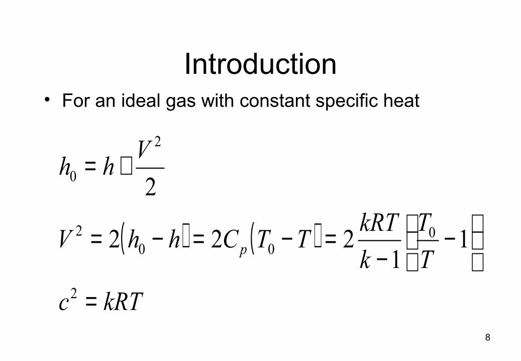
Introduction
( ) ( )
kRTc
T
T
k
kRTTTChhV
Vhh
p
=
−
−=−=−=
+=
2
000
2
2
0
11
222
2
• For an ideal gas with constant specific heat

9
Introduction
20
022
2
02
2
2
11
11
2
11
2
Mk
T
T
T
T
kM
c
V
T
T
k
cV
−+=
−
−==
−
−=
• For an ideal gas with constant specific heat

10
Introduction
( ) ( )
( ) ( )
( ) ( )1120
120
0
11
00
1
0
2
11
2
11
,
−
−
−−
−+=
−+=
=
=
k
kk
kkk
Mk
Mk
p
p
T
T
p
p
T
T
ρρ
ρρ
• For an isentropic process

11
Introduction
( )
( )11
0
*
1
0
*
0
*
1
2
1
2
1
2
−
−
+=
+=
+=
k
kk
k
kp
p
kT
T
ρρ
• For the critical state (M=1)
12
Introduction

13
Introduction
( ) 220103 ′=−= tm VUhhE η
s
1
2
3
p1
p2
p3
p03
0302
01
p02
i
i’h
2
21V

14
Introduction
• The Specific Shaft Work into the Compressor
The specific shaft work
0.96
m
m
E η
η
=
=
15
Introduction
• Compressor Efficiency:– The ratio of the useful increase of fluid energy divided by the
actual energy input to the fluid
– The useful energy input is the work of an ideal, or isentropic, compression to the actual final pressure P3

16
Introduction
[ ]( )
−
=
−=−=−
1
1
1
01
0301
010101
kk
p
ipii
p
pTC
TTTChhE

17
Introduction
0103
01
TT
TT
E
E iic −
−==η
• The Compressor Efficiency
• No external work or heat associated with the diffuser flow, i.e.
03020302 , TThh ==

18
Introduction
1
01
'22
01
03 1
−
+=
kk
mp
ct
TC
VU
p
p
ηη
• The Overall Pressure Ratio
• The compressor efficiency from experimental data• Slip exists in compressor impeller
2'2 tst VV µ=

19
Introduction
−
−=22 cot1
163.01
βϕπµ
Bs n
• The Slip Coefficient (Stanitz Equation)
• More relations in Appendix E• But, Stanitz equation is more accurate for the practical
range of vane angle; i.e.
02
0 9045 << β

20
Introduction
• Total pressure ratio from:– Ideal velocity triangle at the impeller exit– The number of vanes– The inlet total temperature– The stage and mechanical efficiencies
• Mechanical efficiency accounts for– Frictional losses associated with bearing, seal, and disk
friction– Reappears as enthalpy in the outflow gas

21
Impeller Design
• The impeller design starts with a number of unshrouded blades (Pfleiderer)
• Flow is assumed axial at the inlet• Favorable to have large tangential velocity at outlet
(Vt2’)
• Vanes are curved near the rim of the impeller (β2 <90o)
• But, they are bent near the leading edge to conform to the direction of the relative velocity Vrb1 at the inlet

22
Impeller Design
• The angle β1 varies over the leading edge, since V1 remains constant while U1 (and r) varies (V1 assumes uniform at inlet)
• At D1S, the relative velocity Vrb1=(V12+U1
2)0.5 and the corresponding relative Mach number MR1S are highest
• For a fixed set of, N, m,Po1, and To1, the relative Mach number has its minimum where β1S is approximately 32o (Shepherd, 1956)
23
Impeller Design
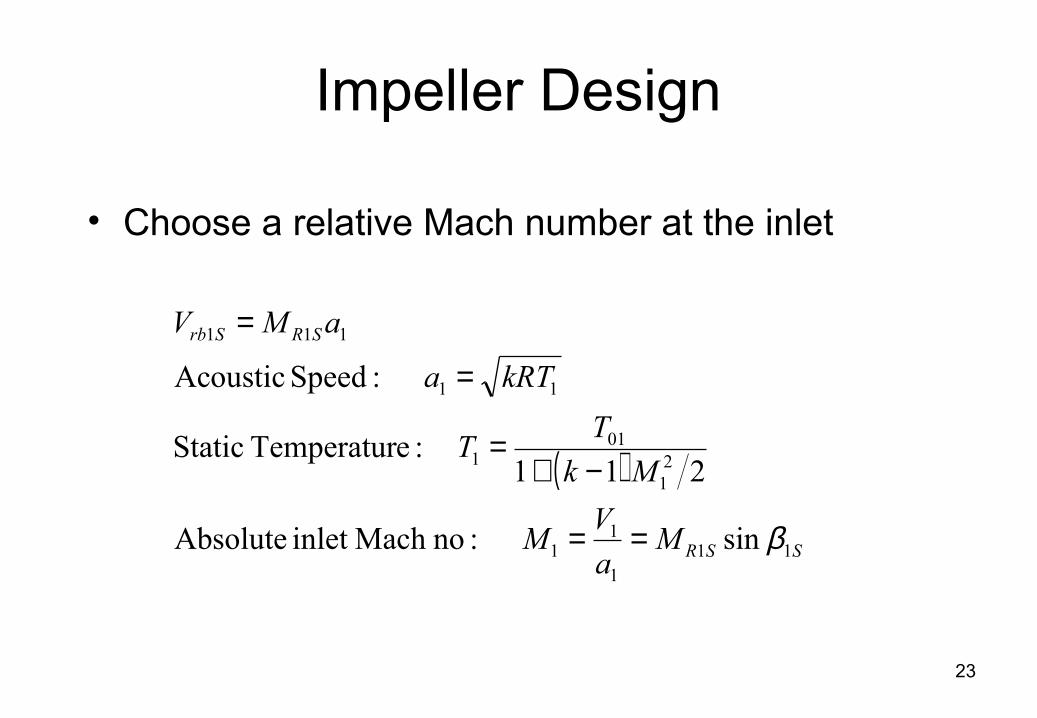
• Choose a relative Mach number at the inlet
( )
SSR
SRSrb
Ma
VM
Mk
TT
kRTa
aMV
111
11
21
011
11
111
sin :noMach inlet Absolute
211 :eTemperatur Static
:Speed Acoustic
β==
−+=
=
=

24
Impeller Design
011
011
32cos
32sin
SrbS
Srb
VU
VV
=
=• Calculation of V1 and U1S
• Calculation of the shroud diameter
N
UD S
S1
1
2=

25
Impeller Design
21
11
211
4
−=
V
mDD SH πρ
• Calculation of the hub diameter by applying the mass flow equation to the impeller inlet
• Calculation of density from the equation of state of a perfect gas
1
11 RT
p=ρ

26
Impeller Design
• Calculation of static temperature and static pressure
( )
( )( )1
21
011
21
011
211
211−
−+
=
−+=
kk
Mk
pp
Mk
TT

27
Impeller Design
= −
HH U
V
1
111 tanβ
• The fluid angle at the hub
• The vane speed at the hub
21
1H
H
NDU =

28
Impeller Design
1 1
12
13
4
12
12 1
4
Inlet flow rate:
Output head H:
Dimensional specific speed:
( from Table 3 in appendix A)
i
s
SS
Q m
H E g
NQN
H
D QD D
H
ρ==
=
=
&
• The outlet diameter D2

29
Impeller Design
( )9.085.0 : velocityl tangentiaideal The
: velocityl tangentiaactual The
:nsferEnergy tra The
:Aappendix in 3 Table From
'22
2'2
C
−==
=
=
ss
tt
t
C
im
VV
UEV
EE
µµ
ηη
η
• The ideal and actual tangential velocities
30
Impeller Design
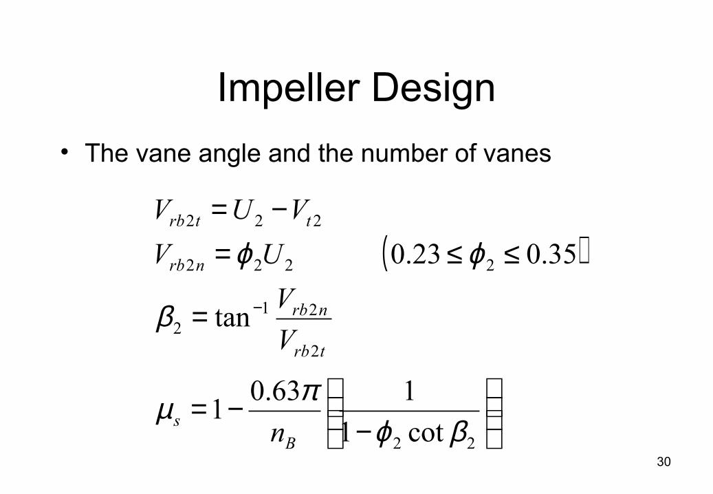
( )
−
−=
=
≤≤=−=
−
22
2
212
2222
222
cot1
163.01
tan
35.023.0
βϕπµ
β
ϕϕ
Bs
trb
nrb
nrb
ttrb
n
V
V
UV
VUV
• The vane angle and the number of vanes
31
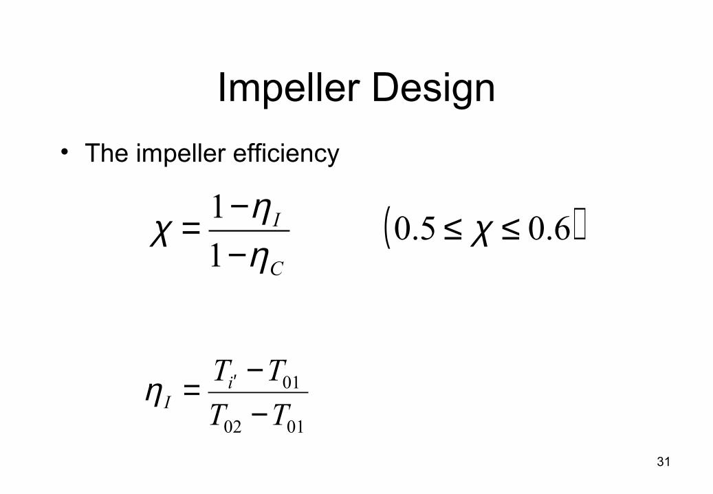
Impeller Design
( )6.05.0 1
1 ≤≤−−= χ
ηηχ
C
I
• The impeller efficiency
0102
01
TT
TTiI −
−= ′η

32
Impeller Design
pC
VTT
2
22
022′−=
• The static temperature T2 is used to determine density at the impeller exit
Vr
mb
n2222 2πρ
&=

33
Impeller Design
• The optimal design parameters by Ferguson (1963) and Whitfield (1990) from Table 5.1
• Table 5.1 Should be used to check calculated results for acceptability during or after the design process

34
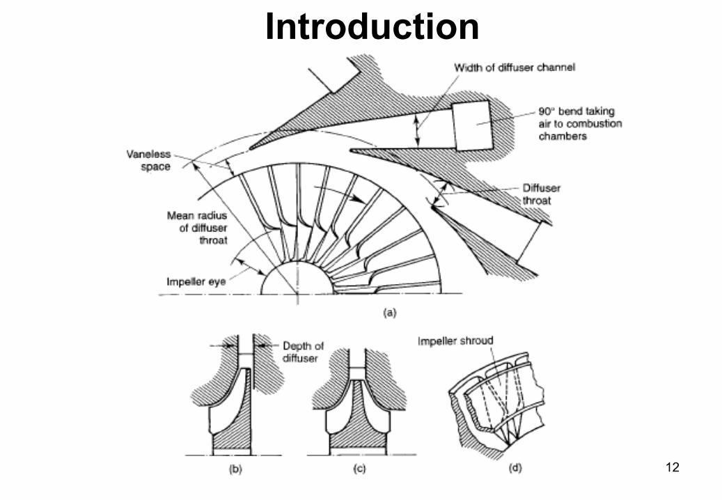
Diffuser Design
• A vaneless diffuser allows reduction of the exit Mach number
• The vaneless portion may have a width as large as 6 percent of the impeller diameter
• Effects a rise in static pressure• Angular momentum is conserved and the fluid path is
approximately a logarithmic spiral• Diffuser vanes are set with the diffuser axes tangent to the
spiral paths with an angle of divergence between them not exceeding 12o

35
Diffuser Design

36
Diffuser Design
• Vanes are preferred where size limitations matter
• Vaneless diffuser is more efficient
• Number of diffuser vanes should be less than the number of impeller vanes to:– Ensure uniformness of flow
– High diffuser efficiency in the range of φ2 recommended

37
Diffuser Design
• The mass flow rate at any r (in the vaneless diffuser)
( )n
nr
Vrbm
rrrVV
ρπ2
32
=≤≤=
&

38
Diffuser Design
222
constant
nn
n
VrrV
rV
ρρρ
==
• For constant diffuser width b
• The angular momentum is conserved in the vaneless space
22 ′= tt VrrV

39
Diffuser Design
12 >′M• Typically, the flow leaving the impeller is supersonic
• Typically, the flow leaving the vaneless diffuser is subsonic
0.13 <M

40
Diffuser Design
αcosVVV nr ==
• Denote * for the properties at the radial position at which M=1 (The absolute gas angle, α, is the angle between V and Vr)
• The continuity equation
**** coscos αραρ VrrV =

41
Diffuser Design
*
*tantan
ρα
ρα =
• The angular momentum equation
• Dividing momentum by continuity relations
*** sinsin αα VrrV =

42
Diffuser Design
2
0
1
**
21
1 ,
Mk
TT
T
Tk
−+=
=−
ρρ
• Assuming an isentropic flow in the vaneless region
• For M=1
1
2 0*
+=
k
TT

43
Diffuser Design
( )11
2* 2
11
1
2−
−+
+=
k
Mk
kρρ
• Substituting in the density relation
• Substituting in the absolute gas angle relation
( )11
2*
2
11
1
2tantan
−−
−+
+=
k
Mk
kαα

44
Diffuser Design
21
2**
21
***
**
2
2
2
11
1
2
sin
sin
sin
sin
−
′
′
−+
+=
===
==
Mk
kM
r
r
T
TM
a
a
a
V
V
V
r
r
MM
αα
αα
αα• The angle α* is evaluated by

45
Diffuser Design
21
222
22
**
2
11
1
2
sin
sin−
′′
−+
+= M
k
kM
r
r
αα
• The radial position r* is determined by
• The angle α3* is evaluated by
( )112
3*
3 2
11
1
2tantan
−−
−+
+=
k
Mk
kαα
46
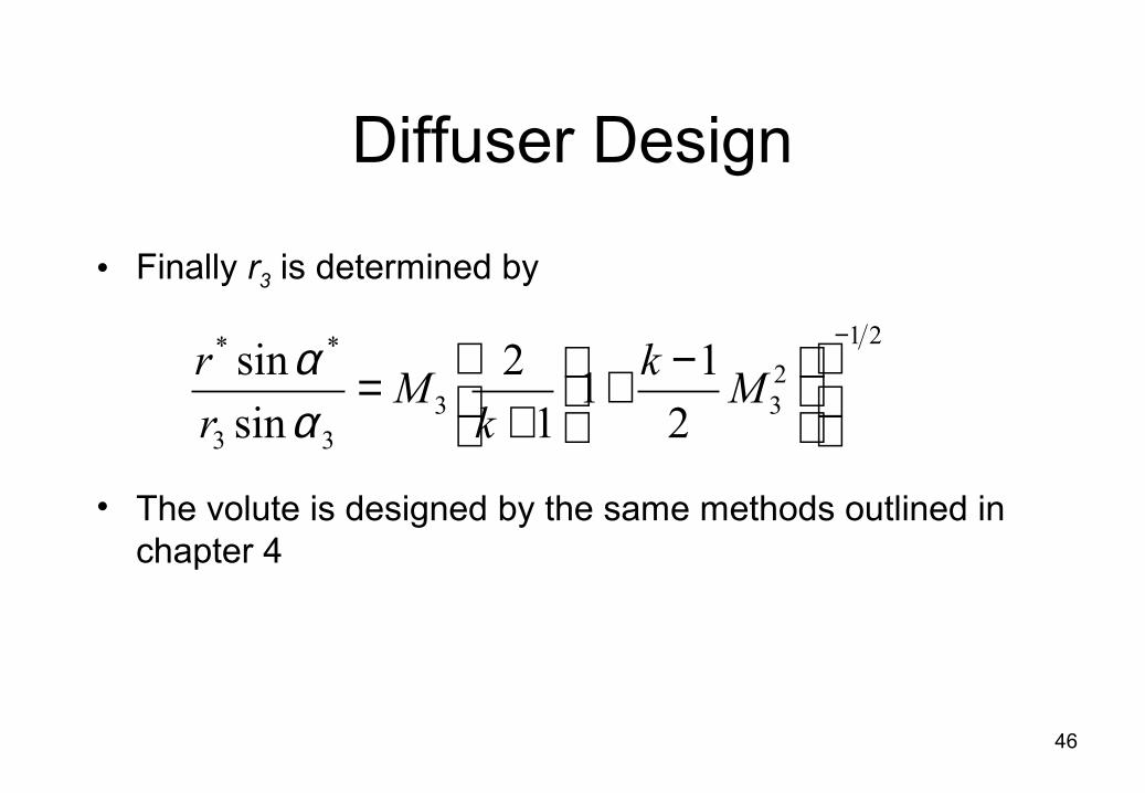
Diffuser Design
21
233
33
**
2
11
1
2
sin
sin−
−+
+= M
k
kM
r
r
αα
• Finally r3 is determined by
• The volute is designed by the same methods outlined in chapter 4

47
Performance• Typical compressor characteristics
cte.01
=T
N
01
01
p
Tm&
02
01
p
p Surge line
.cte=ηmaxη
Choke line
C B
A

48
Performance
• The sharp fall of the constant-speed curves at higher mass flows is due to choking in some component of the machine
• The low flows operation is limited by the phenomenon of surge
• Smooth operation occurs on the compressor map at some point between the surge line and the choke line
• Chocking is associated with the attainment of a Mach number of unity

49
Performance
• In the stationary passage of the inlet The sharp fall of the constant-speed curves at higher mass flows is due to choking in some component of the machine
• The low flows operation is limited by the phenomenon of surge
• Smooth operation occurs on the compressor map at some point between the surge line and the choke line
• Chocking is associated with the attainment of a Mach number of unity

50
Performance
• In the stationary passage of the inlet or diffuser for a Mach number of unity
a =
a kRT=• The temperature at this point
( ) 20
11
2
kT T M
−= +

51
Performance
• By setting M=1
a =
12
t tt
km A p
RT
= ÷
&
• The chocking (maximum) flow rate
*0
2
1 tT T Tk
= = +

52
Performance
• The throat pressure (isentropic process)
a =
2 21 1
01 2 2rbV U
h h= + −
• The chocked flow rate in impeller (use relative velocity instead of absolute velocity)
( )1k k
tt in
in
Tp p
T
−
= ÷

53
Performance
• The critical temperature
a =
( )( )
11
2 12 2
0101 01
21
1 2
k
k
tp
k Um A p
RT k C T
+−
= + ÷ ÷ ÷+ &
• The throat mass flow rate (isentropic process)
( )2
* 01
01
21
2 1 tp
TUT T
C T k
= + = ÷ ÷ +

54
Performance
• The chocked mass flow rate in stationary components is independent of impeller speed
• The point A in the characteristic curve represents a point of normal operation
• An increase in flow resistance in the connected external flow system results in decrease in and increase in
• Causes increase in head or pressure• Further increase in external system produces a decrease in
impeller flow (beyond point C) and surge phenomena results
2nV
2tV

55
Performance
• The at some point in the impeller leads to change of direction of and an accompanying decrease in head.
• A temporary flow reversal in the impeller and the ensuing buildup to the original flow condition is known as surging.
• Surging continues cyclically until the external resistance is removed.
• Surging is an unstable and dangerous condition and must be avoided by careful operational planning and system design.
2rbV

56
Example 5.1

57
Example 5.1

58
Example 5.1

59
Example 5.1

60
Example 5.1

61
Example 5.1

62
Example 5.1
63
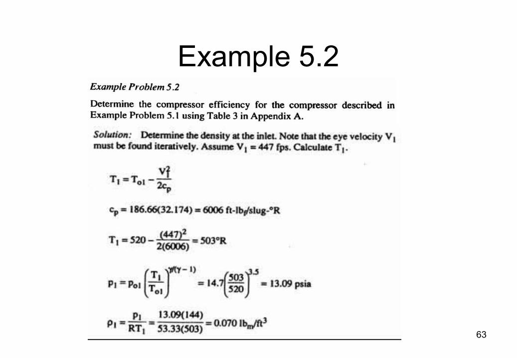
Example 5.2

64
Example 5.2

65
Example 5.2

66
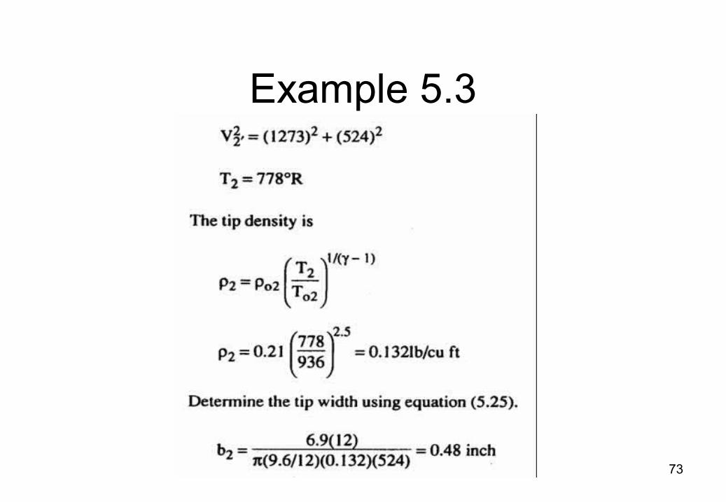
Example 5.3

67
Example 5.3

68
Example 5.3

69
Example 5.3

70
Example 5.3

71
Example 5.3

72
Example 5.3
73
Example 5.3

74
Example 5.3

75
Example 5.3

76
Practice- Sheet 3

77
Practice- Sheet 3

78
TURBOMACHINERY BASICSCENTRIFUGAL COMPRESSOR
Hasan Basri
Jurusan Teknik MesinFakultas Teknik – Universitas Sriwijaya
Phone: 0711-580739, Fax: 0711-560062Email: [email protected]

79

80
EULER EQUATION
Torque T = m (Cθ2r2 – Cθ1r1)
Power P = Tω = m (U2Cθ2 – U1Cθ1)

81
RELAVANT UNIT

82
PREWHIRL OR PREROTATION
83
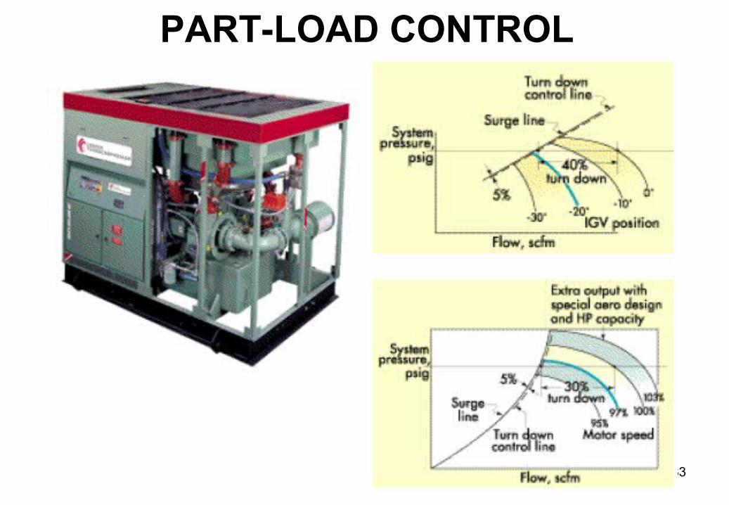
PART-LOAD CONTROL

84
SLIP FACTOR

85
IMPELLER EXIT BLADE ANGLE

86
EFFICIENCY

87
ROTHALPY & TOTAL ENTHALPY

88
ENERGY TRANSFER

89
SPECIFIC SPEED

90

91

92

93
VANED DIFFUSER

94
VANED DIFFUSER

95
LSD (Low Solidity Diffuser)

96
AXIAL VANED DIFFUSER
97
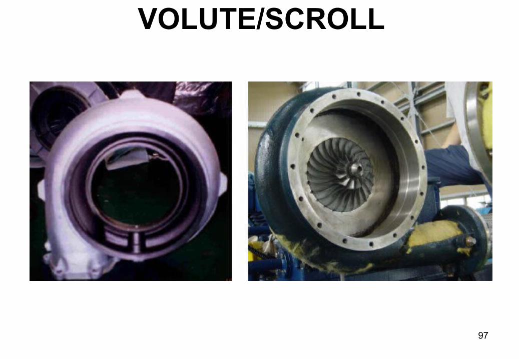
VOLUTE/SCROLL

98
PERFORMANCE MAP

99
PERFORMANCE MAP

100
CORRECTED CONDITIONS

101
IMPELLER INCIDENCE

102
DIFFUSER INCIDENCE

103
SPLITTER BLADES

104
SPLITTER BLADES

105
IMPELLER BLADE GEOMETRY
106
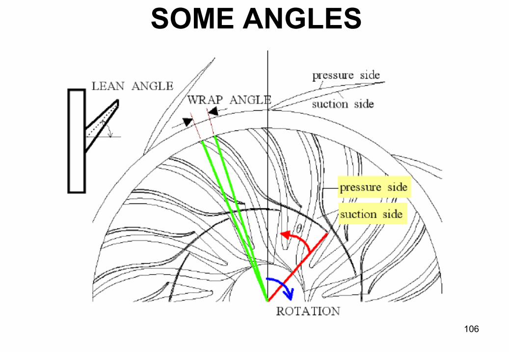
SOME ANGLES

107
IMPELLER CFD

108