
Peloni, Alessandro (2018) asteroid rendezvous.theses.gla.ac.uk/8901/1/2018PeloniPhd.pdfTABLE OF...
233
Peloni, Alessandro (2018) Solar-sail mission design for multiple near-Earth asteroid rendezvous. PhD thesis. https://theses.gla.ac.uk/8901/ Copyright and moral rights for this work are retained by the author A copy can be downloaded for personal non-commercial research or study, without prior permission or charge This work cannot be reproduced or quoted extensively from without first obtaining permission in writing from the author The content must not be changed in any way or sold commercially in any format or medium without the formal permission of the author When referring to this work, full bibliographic details including the author, title, awarding institution and date of the thesis must be given Enlighten: Theses https://theses.gla.ac.uk/ [email protected]
Transcript of Peloni, Alessandro (2018) asteroid rendezvous.theses.gla.ac.uk/8901/1/2018PeloniPhd.pdfTABLE OF...

Peloni, Alessandro (2018) Solar-sail mission design for multiple near-Earth
asteroid rendezvous. PhD thesis.
https://theses.gla.ac.uk/8901/
Copyright and moral rights for this work are retained by the author
A copy can be downloaded for personal non-commercial research or study,
without prior permission or charge
This work cannot be reproduced or quoted extensively from without first
obtaining permission in writing from the author
The content must not be changed in any way or sold commercially in any
format or medium without the formal permission of the author
When referring to this work, full bibliographic details including the author,
title, awarding institution and date of the thesis must be given
Enlighten: Theses
https://theses.gla.ac.uk/

SOLAR-SAIL MISSION DESIGN FOR
MULTIPLE NEAR-EARTH ASTEROID
RENDEZVOUS
ALESSANDRO PELONI
Submitted in fulfilment of the requirements for the Degree of Doctor of Philosophy
School of Engineering College of Science and Engineering
University of Glasgow
© 2018 Alessandro Peloni

II
Alessandro Peloni: Solar-sail mission design for multiple near-Earth asteroid rendezvous
Submitted in fulfilment of the requirements for the Degree of Doctor of Philosophy
School of Engineering, College of Science and Engineering
University of Glasgow
© 2018 Alessandro Peloni
ADVISOR:
Dr Matteo Ceriotti
EXAMINERS:
Dr Roberto Armellin
Surrey Space Centre, University of Surrey
Guilford, United Kingdom
Dr Patrick Harkness
School of Engineering, University of Glasgow
Glasgow, United Kingdom
Glasgow, Scotland, United Kingdom
06 March 2018

III
ABSTRACT
Solar sailing is the use of a thin and lightweight membrane to reflect sunlight
and obtain a thrust force on the spacecraft. That is, a sailcraft has a potentially-
infinite specific impulse and, therefore, it is an attractive solution to reach
mission goals otherwise not achievable, or very expensive in terms of propellant
consumption. The recent scientific interest in near-Earth asteroids (NEAs) and the
classification of some of those as potentially hazardous asteroids (PHAs) for the
Earth stimulated the interest in their exploration. Specifically, a multiple NEA
rendezvous mission is attractive for solar-sail technology demonstration as well as
for improving our knowledge about NEAs. A preliminary result in a recent study
showed the possibility to rendezvous three NEAs in less than ten years. According
to the NASA’s NEA database, more than 12,000 asteroids are orbiting around the
Earth and more than 1,000 of them are classified as PHA. Therefore, the selection
of the candidates for a multiple-rendezvous mission is firstly a combinatorial
problem, with more than a trillion of possible combinations with permutations of
only three objects. Moreover, for each sequence, an optimal control problem
should be solved to find a feasible solar-sail trajectory. This is a mixed
combinatorial/optimisation problem, notoriously complex to tackle all at once.
Considering the technology constraints of the DLR/ESA Gossamer roadmap, this
thesis focuses on developing a methodology for the preliminary design of a mission
to visit a number of NEAs through solar sailing. This is divided into three sequential
steps. First, two methods to obtain a fast and reliable trajectory model for solar
sailing are studied. In particular, a shape-based approach is developed which is
specific to solar-sail trajectories. As such, the shape of the trajectory that
connects two points in space is designed and the control needed by the sailcraft

Abstract IV
to follow it is analytically retrieved. The second method exploits the homotopy
and continuation theory to find solar-sail trajectories starting from classical low-
thrust ones. Subsequently, an algorithm to search through the possible sequences
of asteroids is developed. Because of the combinatorial characteristic of the
problem and the tree nature of the search space, two criteria are used to reduce
the computational effort needed: (a) a reduced database of asteroids is used
which contains objects interesting for planetary defence and human spaceflight;
and (b) a local pruning is carried out at each branch of the tree search to discard
those target asteroids that are less likely to be reached by the sailcraft
considered. To reduce further the computational effort needed in this step, the
shape-based approach for solar sailing is used to generate preliminary trajectories
within the tree search. Lastly, two algorithms are developed which numerically
optimise the resulting trajectories with a refined model and ephemerides. These
are designed to work with minimum input required by the user. The shape-based
approach developed in the first stage is used as an initial-guess solution for the
optimisation.
This study provides a set of feasible mission scenarios for informing the
stakeholders on future mission options. In fact, it is shown that a large number of
five-NEA rendezvous missions are feasible in a ten-year launch window, if a solar
sail is used. Moreover, this study shows that the mission-related technology
readiness level for the available solar-sail technology is larger than it was
previously thought and that such a mission can be performed with current or at
least near-term solar sail technology. Numerical examples are presented which
show the ability of a solar sail both to perform challenging multiple NEA
rendezvous and to change the mission en-route.

TABLE OF CONTENTS
ABSTRACT ....................................................................... III
TABLE OF CONTENTS ............................................................. V
LIST OF FIGURES ............................................................... VIII
LIST OF TABLES ................................................................. XI
LIST OF ALGORITHMS ........................................................... XIII
ACKNOWLEDGEMENTS ......................................................... XIV
PUBLICATIONS AND CONFERENCES ............................................. XVII
AUTHOR’S DECLARATION ....................................................... XX
NOMENCLATURE ................................................................XXI
CHAPTER 1. INTRODUCTION .................................................... 1
1.1. Solar-Sail Mission Design for Multiple NEA
Rendezvous: An Overview ......................................... 1
1.2. Objectives ........................................................... 4
1.3. Outline ............................................................... 6
CHAPTER 2. SURVEY OF THEORY AND METHODS ............................... 8
2.1. Solar Sailing from the Ground Up ................................ 8
2.1.1. Solar Radiation Pressure: From Maxwell to Einstein ................. 8
2.1.2. Acceleration Model ...................................................... 12
2.1.3. Solar Sailing from the 1970s to the Present Day .................... 16
2.2. Techniques for Space Trajectory Optimisation ............... 18
2.2.1. Indirect Methods ......................................................... 20
2.2.2. Direct Methods ........................................................... 23
2.2.3. Metaheuristic Optimisation Methods .................................. 32
2.2.4. Shape-Based Approaches ............................................... 34
2.2.5. Solar-Sailing Trajectory Design ........................................ 39

Table of Contents VI
2.2.6. Target Selection ......................................................... 40
2.3. Near-Earth Asteroids .............................................. 44
CHAPTER 3. PRELIMINARY SOLAR-SAIL TRAJECTORY DESIGN ................ 47
3.1. Shape-Based Approach for Solar Sailing ....................... 48
3.1.1. Pseudo Modified Equinoctial Elements ............................... 48
3.1.2. Choice of the Shaping Functions ....................................... 51
3.1.3. Study of the Gauge Freedom ........................................... 59
3.1.4. Boundary-Constraint Satisfaction ...................................... 60
3.1.5. Shaped Trajectory and Control History Generation ................. 61
3.1.6. Practical Use of the Shape-Based Approach for Solar
Sailing...................................................................... 63
3.1.7. Assessing the Performances of the Shape-Based
Approach for Solar Sailing .............................................. 67
3.2. From Low Thrust to Solar Sailing: A Homotopic
Approach ........................................................... 72
3.2.1. Mathematical Model ..................................................... 72
3.2.2. Homotopy-Continuation Approach .................................... 76
3.2.3. Numerical Test Cases .................................................... 81
3.3. Discussion ........................................................... 91
CHAPTER 4. ASTEROID SEQUENCE SEARCH ................................... 92
4.1. Asteroid Database Selection ..................................... 93
4.2. Local Pruning on the Database .................................. 99
4.3. Simplified Trajectory Model ................................... 103
4.4. Sequence Search Algorithm .................................... 104
4.5. Application to Gossamer Mission .............................. 107
4.6. Numerical Test Cases ........................................... 108
4.6.1. PHA-NHATS Database ................................................... 108
4.6.2. PHA-LCDB Database .................................................... 119
4.7. Discussion ......................................................... 120
CHAPTER 5. SEQUENCE OPTIMISATION ...................................... 123
5.1. Problem Formulation ........................................... 124
5.2. STO: Sequential Trajectory Optimiser ....................... 127
5.3. ATOSS: Automated Trajectory Optimiser for Solar
Sailing ............................................................. 129

Table of Contents VII
5.3.1. Initial-Guess Generator ................................................ 131
5.3.2. Optimisation Strategy .................................................. 131
5.4. Numerical Test Cases ........................................... 136
5.4.1. Circular-to-Circular Orbit Transfers: A Comparison
with the Literature ..................................................... 136
5.4.2. Three-NEA Rendezvous Mission: A Comparison with
the Literature ........................................................... 138
5.4.3. Multiple NEA Rendezvous Missions .................................... 141
5.4.4. Multiple NEA Sample Return Mission ................................. 151
5.4.5. Online Change of the Mission: Two Test Cases for
the Planetary Defence ................................................. 152
5.4.6. Automated Optimisation Campaign .................................. 159
5.5. Discussion ......................................................... 161
CHAPTER 6. CONCLUSIONS .................................................. 163
6.1. Summary of the Work ........................................... 163
6.2. Summary of the Findings ....................................... 166
6.3. Current Limitations and Future Research ................... 168
6.3.1. Current Limitations ..................................................... 168
6.3.2. Proposed Future Research ............................................. 169
APPENDIX A METAHEURISTIC OPTIMISATION METHODS: A
CLOSER LOOK ................................................. 171
A.1. Genetic Algorithm ............................................... 171
A.2. Particle Swarm Optimisation .................................. 173
A.3. InTrance .......................................................... 175
APPENDIX B IMPLEMENTATION DETAILS ..................................... 177
B.1. MATLAB and C: A Performances Study ....................... 177
B.2. PPSO: Peloni Particle Swarm Optimiser ...................... 179
B.2.1. Test Case 1: Rastrigin’s Function ..................................... 179
B.2.2. Test Case 2: Simple Function of Two Variables .................... 180
B.2.3. Test Case 3: CEC 2005 .................................................. 181
B.2.4. Test Case 4: Optimal Two-Impulsive Transfer
between Two Circular Orbits .......................................... 182
B.2.5. Test Case 5: Bi-Impulsive Earth-Apophis Transfer ................. 183
REFERENCES ................................................................... 185

List of Figures VIII
LIST OF FIGURES
Fig. 2.1. Montage of the Halley’s Comet approaching the Sun in 1910. ........... 9
Fig. 2.2. Sketch of a perfectly-reflecting flat solar sail. ........................... 13
Fig. 2.3. Graphical view of the normal unit vector in the orbital
reference frame and the sail cone and clock angles. ................... 14
Fig. 2.4. Sketch (not to scale) of classical low-thrust vs solar-sail
achievable accelerations. It is evident that the thrust given
by the two propulsion systems is equal only if the sail is
facing the Sun. ................................................................ 16
Fig. 2.5. Schematic of the trajectory structure with a direct shooting
method [75] (Reproduced with permission of AIAA). .................... 26
Fig. 2.6. Lagrange polynomial approximation of the function
41 1 25 using (a) 25 equidistant points and (b) 25 LGR
points. .......................................................................... 27
Fig. 2.7. Schematic of the tree search implementations [171]
(Reproduced with permission of Springer). Dotted lines and
circles indicate branches yet to be explored. Crossed circles
refer to pruned branches. (a) Breadth-first search. (b)
Depth-first search. (c) Beam search. ...................................... 43
Fig. 2.8. NEA discovery statistics. ...................................................... 46
Fig. 3.1. Representation of the trajectory (bold line) as a succession
of points on instantaneous ellipses. The generic case for
which the gauge term is non-zero is shown. .............................. 50
Fig. 3.2. Evolution of the in-plane pMEE F (a) and G (b) over true
longitude under the effect of a constant sail angle. .................... 52
Fig. 3.3. In-plane pMEE F and G over true longitude. ............................... 53
Fig. 3.4. Semilatus rectum over true longitude. ..................................... 55
Fig. 3.5. Earth-Mars coplanar orbit transfer. (a) Semilatus rectum and
(b) in-plane elements F and G over true longitude. ..................... 57
Fig. 3.6. Earth-Mars coplanar orbit transfer. Sail cone angle over true
longitude. ...................................................................... 58
Fig. 3.7. Shape-based approach (Case study 9). Control history found
with (a) shape-based approach – shaped trajectory, and (b)
GPOPS-II with NLP solver WORHP. ......................................... 71
Fig. 3.8. Polar inertial reference frame in the ecliptic plane. .................... 73
Fig. 3.9. Homotopic approach (Test case 1). Control history for
coplanar circular-to-circular Earth-Mars orbit transfer (ac =
1 mm/s2). (a) Cone angle evolution during first
continuation. (b) Low-thrust and solar-sail cone angle
evolution. ...................................................................... 85

List of Figures IX
Fig. 3.10. Homotopic approach (Test case 1). Ecliptic plane view of
the transfer trajectories for coplanar circular-to-circular
Earth-Mars orbit transfer (ac = 1 mm/s2). (a) Low thrust. (b)
Solar sail. ...................................................................... 85
Fig. 3.11. Homotopic approach (Test case 1). (a) Zero-path. (b)
Evolution of . ................................................................. 85
Fig. 3.12. Homotopic approach (Test case 2). Coplanar circular-to-
circular Earth-Mars orbit transfer (ac = 0.1 mm/s2). (a) Cone
angle evolution. (b) Solar-sail transfer trajectory (ecliptic
plane view). ................................................................... 87
Fig. 3.13. Homotopic approach (Test case 2). (a) Zero-path. (b)
Evolution of . ................................................................. 87
Fig. 3.14. Homotopic approach (Test cases 3 and 4). Ecliptic plane
view of the solar-sail transfer trajectories for rendezvous
from Earth to (99942) Apophis. (a) ac = 0.6 mm/s2. (b) ac =
0.12 mm/s2. ................................................................... 89
Fig. 3.15. Homotopic approach (Test case 4). Cone angle evolution
during the second continuation. ............................................ 89
Fig. 3.16. Minimum time of flight as a function of the characteristic
acceleration for the coplanar Earth-Apophis case. ...................... 90
Fig. 4.1. Heliocentric view of the positions of all known NEAs (small
blue dots) and PHAs (large red dots) on 24 March 2017. (a)
Complete database. (b) PHA-NHATS database. Bodies not to
scale. ........................................................................... 95
Fig. 4.2. Distribution of all NEAs in the (𝚼2, -r⨁/a) space. The two
curves represent the circular limit and the Earth tangency
condition. ...................................................................... 97
Fig. 4.3. Schematic of the tree search. ............................................... 99
Fig. 4.4. Heliocentric view of the transfer trajectory. (a) Test case 1.
(b) Test case 2. .............................................................. 102
Fig. 4.5. Graphical view (not to scale) of pruning on longitude of
pericentre: ranges of possible variation of longitude of
pericentre for two objects (a) overlap; (b) do not overlap. .......... 102
Fig. 4.6. Sequence search flowchart. ................................................. 105
Fig. 4.7. Number of unique sequences with at least one PHA and four
encounters as a function of the launch date. PHA-NHATS
database with ac = 0.2 mm/s2 (Test case 1). ............................ 110
Fig. 4.8. Tree graph of first three legs of all timed sequences with
five encounters found for launch date t0 = 30 April 2025
(Test case 1). ................................................................. 112
Fig. 4.9. Number of unique sequences with at least one PHA and
three encounters as a function of the launch date. PHA-
NHATS database with ac = 0.15 mm/s2 (Test case 2). .................. 114

List of Figures X
Fig. 4.10. Number of unique sequences with at least one PHA and
three encounters as a function of the launch date. PHA-
NHATS database with ac = 0.1 mm/s2 (Test case 3). ................... 114
Fig. 4.11. Number of unique sequences with at least one PHA and five
encounters as a function of the launch date. PHA-NHATS
database with ac = 0.3 mm/s2 (Test case 4). ............................ 116
Fig. 4.12. Tree graph of the first three legs of all sequences with five
encounters found for launch date t0 = 26 May 2020 (Test
case 4). The number of sequences that share the same
branch is shown above each of them. .................................... 117
Fig. 4.13. Number of unique sequences with at least one PHA and five
encounters for six runs on the sequence search for launch
date t0 = 28 May 2020 (Test case 4). ...................................... 119
Fig. 4.14. Number of unique sequences with at least one PHA and
three encounters as a function of the launch date. PHA-
LCDB database with ac = 0.2 mm/s2. ..................................... 120
Fig. 5.1. Schematic of the multi-phase problem under consideration. .......... 124
Fig. 5.2. Sequential trajectory optimiser algorithm. ............................... 129
Fig. 5.3. Flowchart of single-phase ATOSS’ optimisation strategy for
the first stage. ............................................................... 132
Fig. 5.4. Flowchart of both single- and multi-phase ATOSS’
optimisation strategy for the second stage. ............................. 134
Fig. 5.5. Flowchart of multi-phase ATOSS’ optimisation strategy for
the first stage. ............................................................... 135
Fig. 5.6. Optimal orbit transfers in the heliocentric ecliptic reference
frame. (a) Earth-Venus. (b) Earth-Mars. ................................. 137
Fig. 5.7. Trajectory of the first leg from Earth to 2004 GU9.
Heliocentric ecliptic reference frame. (a) Ref. [16]
(Reproduced with permission of Springer). (b) ATOSS with
timed sequence as an input. ............................................... 140
Fig. 5.8. Heliocentric view of the 3D trajectory of optimised sequence
1: (a) ecliptic plane view; (b) 3D view. .................................. 144
Fig. 5.9. Acceleration components history on each transfer leg of
optimised sequence 1. ...................................................... 145
Fig. 5.10. Sail slew rate (a) and sail angular acceleration (b) over
time on the last leg of optimised sequence 1. .......................... 146
Fig. 5.11. Evolution of the total mission duration within ATOSS for
optimised sequence 1. ...................................................... 148
Fig. 5.12. Heliocentric view of the complete three-dimensional
trajectory of optimised sequence 2 (ecliptic plane view). ............ 150
Fig. 5.13. Heliocentric view of the 3D return leg to the Earth. .................. 151
Fig. 5.14. Heliocentric view of the 3D transfer leg between 2008 EV5
and 2011 AG5. ................................................................ 154
Fig. 5.15. Heliocentric view of the coplanar transfer between 2015
JF11 and 2017 PDC (ac = 0.73 mm/s2). .................................... 157

List of Tables XI
Fig. 5.16. Heliocentric view of the 3D transfer trajectory to flyby
2017 PDC. ..................................................................... 159
Fig. A.1. Schematic of the GA’s evolution process. ................................ 172
Fig. A.2. Schematic of position and velocity evolution implemented
within PSO. The next position of each particle is influenced
by the current velocity, the location of its current personal
best solution pbest, and the location of the current best
solution of the swarm gbest [235]. ......................................... 174
Fig. A.3. Schematic of trajectory optimisation using the evolutionary
neurocontroller implemented within InTrance [117]. .................. 176
Fig. B.1. Computational times needed for the computation of the first
leg of the asteroid sequence search considering four
different implementations of the shape-based approach. ............ 178
LIST OF TABLES
Table 2.1. Compendium of shape-based approaches proposed in the
literature. ...................................................................... 38
Table 3.1. Statistical values of the fits for the pMEE P, F, and G. ................ 56
Table 3.2. Earth-Mars coplanar orbit transfer. Statistical values of the
fits for the pMEE P, F, and G. ............................................... 58
Table 3.3. Properties of the objects considered for the single-leg
rendezvous missions. ......................................................... 69
Table 3.4. Case studies for the single-leg rendezvous missions. .................. 69
Table 3.5. Number of successful cases for each initial guess. ..................... 70
Table 3.6. Number of successful cases for each initial guess and NLP
solver. .......................................................................... 70
Table 3.7. Homotopic approach: numerical test cases. ............................ 82
Table 3.8. Homotopic approach: Keplerian elements of the target
objects on 14 Feb 2016. The inclination of both objects is
assumed equal to zero. ...................................................... 82
Table 3.9. Homotopic approach: homotopy and GA results comparison
(Test case 1). .................................................................. 84
Table 3.10. Homotopic approach: homotopy and GA results
comparison (Test case 2). ................................................... 86
Table 3.11. Optimal solar-sail rendezvous from Earth to (99942)
Apophis (in brackets the values from [211]). ............................. 88

List of Tables XII
Table 4.1. Characteristics of the two reduced databases considered. ........... 95
Table 4.2. Number of Q-permutations of N objects within the
complete database and the reduced ones. ............................... 98
Table 4.3. PHA-NHATS database: test cases for the sequence search
algorithm. ..................................................................... 109
Table 5.1. Properties of all the encounters of the sequence presented
in [16]. ........................................................................ 138
Table 5.2. Mission parameters for the optimal 3-NEA rendezvous
(values in brackets are those presented in [16] and used as
timed sequence for ATOSS). ............................................... 140
Table 5.3. Mission parameters for the optimal 3-NEA rendezvous,
longer mission (values in brackets are those presented in
[16] and used as timed sequence for ATOSS). ........................... 140
Table 5.4. Mission parameters for the optimal 3-NEA rendezvous in
the case of a non-timed sequence as an input (values in
brackets are those self-generated by ATOSS). .......................... 141
Table 5.5. Properties of the encounters of sequence 1. ........................... 142
Table 5.6. Mission parameters for optimised sequence 1 (values in
brackets are those found through the sequence search
algorithm and used as a first guess for ATOSS). ......................... 143
Table 5.7. Properties of the encounters of sequence 2. ........................... 149
Table 5.8. Mission parameters for optimised sequence 2 (values in
brackets are the ones found through the sequence search
algorithm and used as an initial guess for STO). ........................ 149
Table 5.9. Mission parameters for the optimised sequence 1 with the
last leg to the Earth. ........................................................ 152
Table 5.10. Properties of 2011 AG5. .................................................. 153
Table 5.11. Mission parameters for optimised sequence 1 with the
last leg to 2011 AG5. ........................................................ 155
Table 5.12. Properties of 2017 PDC. .................................................. 156
Table 5.13. Mission parameters for the baseline mission for the 2017
PDC test case. ................................................................ 156
Table 5.14. Mission parameters for the baseline mission for the 2017
PDC test case with the last leg to 2017 PDC. ............................ 158
Table 5.15. Automated optimisation campaign results. ........................... 161
Table B.1. PPSO Test Case 1: Non-default settings. ................................ 180
Table B.2. PPSO Test Case 1: Results. ................................................ 180
Table B.3. PPSO Test Case 2: Non-default settings. ................................ 181
Table B.4. PPSO Test Case 2: Results. ................................................ 181
Table B.5. PPSO Test Case 3: Results. ................................................ 182
Table B.6. PPSO Test Case 4: Non-default settings. ................................ 183
Table B.7. PPSO Test Case 4: Results. ................................................ 183
Table B.8. PPSO Test Case 5: Non-default settings. ................................ 184
Table B.9. PPSO Test Case 5: Results. ................................................ 184

List of Algorithms XIII
LIST OF ALGORITHMS
Algorithm 3.1. Shape-based approach for solar sailing. Procedure to
generate the shaped trajectory and the control history. ............... 63
Algorithm 3.2. Shape-based approach for solar sailing. Procedure to
generate the shaped trajectory and the control history in
the case of an orbit transfer. ............................................... 67
Algorithm 3.3. Homotopy-continuation approach. .................................. 79
Algorithm 4.1. Sequence search algorithm. ......................................... 106

ACKNOWLEDGEMENTS
This thesis is the result of my four-year work at the University of Glasgow,
beyond the Wall. Several people helped and guided me throughout this wonderful
experience and I am grateful to all of them.
Firstly, I would like to give my heartfelt thanks to Dr Matteo Ceriotti, my PhD
advisor and mentor. He has always been supportive and helpful both inside and
outside the academic environment. He is always ready and happy to help and he
has been my guide during this whole experience. Even though not officially
recognised, he is definitely THE research supervisor of the year 2016.
I would like to acknowledge the Engineering and Physical Sciences Research
Council (EPSRC) for funding my PhD study under the James Watt Program and the
School of Engineering at the University of Glasgow for hosting me. Specifically,
Mrs Elaine McNamara and Ms Heather Lambie have always been kind and willing
to help me in all circumstances here at the university.
I would like to thank Prof Bernd Dachwald for the support he gave during my
research. His insights were of great help towards the achievement of my research
goal and the publication of several journal papers.
I am thankful to Prof Anil Rao, who has been keen to help me since the very
first day I decided to use GPOPS-II. Moreover, he kindly hosted me for four months
at the Vehicle Dynamics and Optimization Laboratory at the University of Florida
as part of his group. Speaking with him is always a pleasure and productive.
I would like to acknowledge the Royal Society of Edinburgh and the University
of Glasgow for supporting my period in Florida and giving me such a fantastic
opportunity.
Special thanks go to Mr Jan Thimo Grundmann. Since we met in Frascati, he
surrounded me with his enthusiasm about solar sailing. He saw the relevance of
my work and helped me spreading it among the scientific community. I hope that
this thesis will help you advance a little in the solar-sail project you guys are
carrying out in the background at DLR.

Acknowledgements XV
Thanks to Prof Christian Circi, who introduced me to the solar-sailing world.
Without his initial advice, this entire PhD would not have existed.
I feel grateful to the several anonymous reviewers and journal editors who
spent their time reviewing my papers. Their feedback and suggestions helped to
improve the overall quality of my research.
I would like to thank all my friends from the Space Glasgow group here at the
University of Glasgow; Leonel (and Luz), Kim, Abdul, Spencer, Alisha, Chen, Yohei,
Callum, Federica, and all the people who have been part of the group even for a
few months only. Of course, Prof Colin McInnes, who welcomed me within his
group and shared with me several interesting and useful insights. His knowledge
and interest in everything related to physics, engineering and, naturally, solar
sailing inspire me.
Among all the people I met here, special thanks go to Nicola, colleague, friend,
and flatmate. He listens to all my monologues about everything, from my research
to my life. Without him, my life here and my research would have definitely been
different.
Thanks to my first crew here at the university; Sotos (and Athina), David,
Fernando, and Juan. They helped me to start my new life here and, definitely,
improve my communication skills in English! Likewise, thanks to my following
officemates, with whom I shared the joys (and sufferings) of our PhD life; Aaron,
Anggoro, Daniel, Helen, Sean, and Lin Wei.
Thanks to their daily support and patience to my life friends Fabrizio, Stefano
and Daniele. I owe you a dram!
Nilay. The love of my life. This thesis is also the result of her love and support.
She always believes in me even when I do not and she led me towards this point.
I cannot be happier to have her in my life.
Lastly, I am truly grateful to my family for supporting me in all my choices.
Especially my mum and dad, who accepted, encouraged and helped this very
decision of mine to pursue this PhD here in Glasgow. Thanks to them, I became
who I am today.
Alessandro Peloni

To my mum and dad,
For their constant love and support.
PUBLICATIONS AND CONFERENCES
The content of this thesis has previously appeared, or will appear, in the
following publications and conferences.
JOURNAL ARTICLES
Peloni, A., Ceriotti, M. and Dachwald, B., “Solar-Sail Trajectory Design for a
Multiple Near-Earth-Asteroid Rendezvous Mission”, Journal of Guidance, Control,
and Dynamics, Vol. 39, No. 12, 2016, pp. 2712-2724. DOI: 10.2514/1.G000470.
Sullo, N., Peloni, A. and Ceriotti, M., “Low-Thrust to Solar-Sail Trajectories: A
Homotopic Approach”, Journal of Guidance, Control, and Dynamics, Vol. 40, No.
11, 2017, pp. 2796-2806. DOI: 10.2514/1.G002552.
Peloni, A., Dachwald, B. and Ceriotti, M., “Multiple Near-Earth Asteroid
Rendezvous Mission: Solar-Sailing Options”, accepted for publication in Advances
in Space Research. DOI: 10.1016/j.asr.2017.10.017.
Peloni, A., Rao, A. V. and Ceriotti, M., “Automated Trajectory Optimizer for
Solar Sailing (ATOSS)”, Aerospace Science and Technology, Vol. 72, 2018, pp. 465-
475. DOI: 10.1016/j.ast.2017.11.025.
Grundmann, J. T., Bauer, W., Biele, J., Boden, R. C., Ceriotti, M., Cordero,
F., Dachwald, B., Dumont, E., Grimm, C. D., Herčík, D., Ho, T. M., Jahnke, R.,
Koch, A. D., Koncz, A., Krause, C., Lange, C., Lichtenheldt, R., Maiwald, V.,
Mikschl, T., Mikulz, E., Montenegro, S., Pelivan, I., Peloni, A., Quantius, D.,
Reershemius, S., Renger, T., Riemann, J., Ruffer, M., Sasaki, K., Schmitz, N.,
Seboldt, W., Seefeldt, P., Spietz, P., Spröwitz, T., Sznajder, M., Tardivel, S.,
Tóth, N., Wejmo, E., Wolff, F., Ziach, C., “Capabilities of GOSSAMER-1 derived
Small Spacecraft Solar Sails carrying MASCOT-derived Nanolanders for In-Situ
Surveying of NEAs”, accepted for publication in Acta Astronautica. DOI:
10.1016/j.actaastro.2018.03.019.

Publications and Conferences XVIII
CONFERENCE PROCEEDINGS
Peloni, A., Ceriotti, M. and Dachwald, B., “Preliminary Trajectory Design of a
Multiple NEO Rendezvous Mission Through Solar Sailing”, 65th International
Astronautical Congress, IAF Paper IAC-14-C1.9.7, Toronto, Canada, 2014.
Peloni, A., Ceriotti, M. and Dachwald, B., “Solar-Sailing Trajectory Design for
Close-up NEA Observations Mission”, 4th IAA Planetary Defense Conference - PDC
2015, IAA Paper IAA-PDC-15-P-19, Frascati, Italy, 2015.
Sullo, N., Peloni, A. and Ceriotti, M., “From Low Thrust to Solar Sailing: A
Homotopic Approach”, 26th AAS/AIAA Space Flight Mechanics Meeting, AAS Paper
16-426, Napa, CA, USA, 2016.
Peloni, A., Wolz, D., Ceriotti, M. and Althöfer, I., “Construction and
Verification of a Solution of the 8th Global Trajectory Optimization Competition
Problem. Team 13: GlasgowJena+”, 26th AAS/AIAA Space Flight Mechanics
Meeting, AAS Paper 16-425, Napa, CA, USA, 2016.
Grundmann, J. T., Boden, R. C., Ceriotti, M., Dachwald, B., Dumont, E.,
Grimm, C. D., Lange, C., Lichtenheldt, R., Pelivan, I., Peloni, A., Riemann, J.,
Spröwitz, T. and Tardivel, S., “Soil to Sail - Asteroid Landers on Near-Term
Sailcraft as an Evolution of the GOSSAMER Small Spacecraft Solar Sail Concept for
In-Situ Characterization”, 5th IAA Planetary Defense Conference - PDC 2017, IAA
Paper IAA-PDC-17-05-19, Tokyo, Japan, 2017.
Peloni, A., Dachwald, B. and Ceriotti, M., “Multiple NEA Rendezvous Mission:
Solar Sailing Options”, The Fourth International Symposium on Solar Sailing 2017,
Paper 17017, Kyoto, Japan, 2017.
Grundmann, J. T., Bauer, W., Biele, J., Boden, R. C., Ceriotti, M., Cordero,
F., Dachwald, B., Dumont, E., Grimm, C. D., Herčík, D., Ho, T. M., Jahnke, R.,
Koch, A. D., Koncz, A., Lichtenheldt, R., Maiwald, V., Mikschl, T., Mikulz, E.,
Montenegro, S., Pelivan, I., Peloni, A., Quantius, D., Reershemius, S., Renger, T.,
Riemann, J., Ruffer, M., Schmitz, N., Seboldt, W., Seefeldt, P., Spietz, P.,
Spröwitz, T., Sznajder, M., Tardivel, S., Tóth, N., Wejmo, E., Wolff, F., Ziach, C.,
“Small Spacecraft Solar Sailing for Small Solar System Body Multiple Rendezvous
and Landing”, accepted for 2018 IEEE Aerospace Conference, IEEE Paper 2360, Big
Sky, MT, USA, 2018.

Publications and Conferences XIX
CONFERENCE AND WORKSHOP PRESENTATIONS
Peloni, A. and Ceriotti, M., “Solar Sailing Multiple NEO Rendezvous Mission:
Preliminary Results”, First Stardust Global Virtual Workshop (SGVW-1) on
Asteroids and Space Debris, Glasgow, Scotland, UK, 2014. Presentation available
online at https://www.youtube.com/watch?v=j-uxCvo09Hc [retrieved 06 June
2017].
Peloni, A., “Solar Sailing: How to Travel on a Light Beam”, 1st Space Glasgow
Research Conference, Glasgow, Scotland, UK, 2014. Presentation available online
at https://www.gla.ac.uk/media/media_375002_en.pptx [retrieved 10 October
2017].
Peloni, A., Rao, A. V. and Ceriotti, M., “ATOSS: Automated Trajectory
Optimiser for Solar Sailing”, Fourth European Optimisation in Space Engineering
(OSE) Workshop, Bremen, Germany, 2017.

AUTHOR’S DECLARATION
I hereby declare that this submission is my own work and that, to the best of
my knowledge and belief, it contains no material previously published or written
by another person nor material which to a substantial extent has been accepted
for the award of any other degree or diploma of the university or other institute
of higher learning, except where due acknowledgment has been made in the text.
Glasgow, Scotland, United Kingdom
06 March 2018
____________________________________
Alessandro Peloni

NOMENCLATURE
The author attempted to use standard symbols and acronyms in use in
Astrodynamics and Optimisation, giving alternatives wherever appropriate, and
tried to be consistent throughout the document. Some symbols have duplicate
meanings but the appropriate one should be clear from the context. The following
notation will be used throughout the document. All scalar quantities will be
represented by non-bold italic symbols. All vectors will be treated as column
vectors and represented by bold italic symbols. Lastly, all matrices will be denoted
by uppercase non-italic bold symbols.
Acronyms
3D = Three Dimensional
ACO = Ant Colony Optimisation
AMR = Area-to-Mass Ratio
ANN = Artificial Neural Network
ARRM = Asteroid Redirect Robotic Mission
ARS = Adjusted R-Square
ATOSS = Automated Trajectory Optimiser for Solar Sailing
AU = Astronomical Unit, 149,597,870.691 km
BFS = Breadth-First Search
BS = Beam Search
CNEOS = Center for Near Earth Object Studies
CR3BP = Circular Restricted Three-Body Problem
DFS = Depth-First Search
DLR = Deutsches zentrum für Luftund Raumafhart e.V. (German
Aerospace Centre)
EMOID = Earth Minimum Orbit Intersection Distance, AU
ESA = European Space Agency

Nomenclature XXII
EXP-TRIG = Exponential Trigonometric
FB = Flyby
FFS = Finite Fourier Series
GA = Genetic Algorithm
GO = Global Optimisation
GTOC = Global Trajectory Optimisation Competition
IAA = International Academy of Astronautics
JPL = Jet Propulsion Laboratory
KEP = Keplerian elements
KKT = Karush-Kuhn-Tucker
LCDB = Lightcurve Database
LG = Legendre-Gauss
LGL = Legendre-Gauss-Lobatto
LGR = Legendre-Gauss-Radau
LIN-TRIG = Linear Trigonometric
LO = Local Optimisation
LT = Low Thrust
MEE = Modified Equinoctial Elements
MTSP = Motorised Travel Salesman Problem
NASA = National Aeronautics and Space Administration
NC = Neurocontroller
NEA = Near-Earth Asteroid
NHATS = Near-Earth object Human space flight Accessible Target Study
NLP = Nonlinear Programming
OCC = Orbit Condition Code
OCP = Optimal Control Problem
ODE = Ordinary Differential Equation
OT = Orbit Transfer
PHA = Potentially-Hazardous Asteroid
pMEE = Pseudo Modified Equinoctial Elements
PDC = Planetary Defense Conference
PSO = Particle Swarm Optimisation
RV = Rendezvous
SB = Shape-Based
SI = International System of Units
Nomenclature XXIII
SRP = Solar Radiation Pressure
SSE = Sum of Squares due to Error
STO = Sequential Trajectory Optimiser
TPBVP = Two-Point Boundary Value Problem
TRL = Technology Readiness Level
TSP = Travel Salesman Problem
Symbols
A x = Matrix of the dynamics
A = Sail area, 2m
, , ,A B C D = Multiplication factors of the Hamiltonian expansion
a = Acceleration vector, 2mm s
ra = Radial component of the acceleration, 2mm s
ta = Transversal component of the acceleration, 2mm s
a = Semimajor axis, AU
ca = Solar-sail characteristic acceleration, 2mm s
ha = Out-of-plane magnitude of the acceleration, 2mm s
maxa = Maximum low-thrust acceleration, 2mm s
0 0,
Pa b = Out-of-plane shaping parameters for the exponential sinusoid
approach
, , , ,, ,a b c d e f g = Shaping parameters for the inverse polynomial shape
B = Magnetic field vector, T
b x = Vector of the dynamics
b = Identifier of a body
c = Vector of the path constraints
c = Speed of light in vacuum, 82.99792 10 m s
, ,I C S
c c c = Inertial, cognitive and social weights
ijD = Differentiation matrix
E = Electric field vector, N C
e = Eccentricity

Nomenclature XXIV
,F G = Pseudo modified equinoctial elements corresponding to f and g
f = Equations of the dynamics
SRPf = Force acting on the sail due to the SRP, N
,SRP if = Force acting on the sail due to the incident radiation, N
,SRP rf = Force acting on the sail due to the reflected radiation, N
f = Generic continuous function
,f g = In-plane modified equinoctial elements
G = Momentum vector (G G ), kgm s
g x = Algebraic constraints
( )k
bestg = Best position vector of the entire swarm of iteration step k
g = Integral cost function
0g = Standard sea level acceleration due to gravity, 29.80665 m s
H = Hamiltonian
H = Reduced Hamiltonian
,H K = Pseudo modified equinoctial elements corresponding to h and k
h = Orbital angular momentum unit vector
,h k = Out-of-plane modified equinoctial elements
= Reduced Planck’s constant, 341.05457 10 Js
K = Number of mesh intervals
maxK = Maximum number of iteration steps
0 1 2, , ,k k k = In-plane shaping parameters for the exponential sinusoid approach
I = Poynting vector, 2W m
spI = Specific impulse, s
i = Inclination, deg
J = Objective (cost) function
j = Phase number
L = Luminosity, W
L = Luminosity of the Sun, 263.8 10 W
L = True longitude, rad
bL = List of available bodies in the database

Nomenclature XXV
,b iL = List of bodies already encountered
complL = List of complete sequences
partL = List of partial sequences
tmpL = List of temporary sequences
ˆf
L = Lower boundary on f
L , rad
j = Lagrange interpolating polynomial at j-th collocation point
m = Number of nonlinear equations of the shooting function
0m = Total spacecraft mass, kg
1m = Number of inequality constraints
drym = Spacecraft dry mass, kg
restm = Mass at rest, kg
N = Acceleration unit vector,
T
r hN N N
N = Number of objects in the database
N = Number of collocation points (CHAPTER 2)
kN = Number of collocation points at k-th mesh interval
max
seqN = Maximum number of partial sequences to be used in the following
leg within the sequence search algorithm
n = Number of optimisation variables
revn = Number of complete revolutions
,
rn n = Number of Fourier terms in the FFS approach
P = Value of the Palermo scale
P = Pseudo modified equinoctial element corresponding to p
P = Solar radiation pressure, 2μN m (CHAPTER 2)
NP = N-th degree Legendre polynomial
N
QP = Number of Q-permutations of N elements
P = Solar radiation pressure at Earth distance, 24.56 N mμ
p = Vector of static parameters
( )k
bestip = Best position vector of particle i at iteration step k
p = Semilatus rectum, AU

Nomenclature XXVI
Q = Number of distinct elements to be considered for the computation
of the permutation
2, ,q s = Auxiliary variables
r = Cartesian position vector ( r r ), AU
r = Position unit vector
( )k ir = Position vector of particle i at iteration step k
r = Mean Sun-Earth distance, 1 AU
ar = Radius of the apocentre, AU
pr = Radius of the pericentre, AU
0,1r = Random number between 0 and 1
is = Partial sequence
T = Pseudo element corresponding to t
T = Effective temperature, K (CHAPTER 2)
0 fT = Time of flight, s
T = Tisserand parameter related to Earth
t = Time, s
0t = Launch date
0t = Selected launch date
stayt = Stay time at the object, s
iU = Discretised control vector at i-th collocation point
U = Set of feasible controls
U = Quality code
u = Control vector
iu = Direction of the incident radiation
ˆr
u = Direction of the reflected radiation
u = Radial velocity, km s
u = Low-thrust non-dimensional control
v = Velocity vector
( )k iv = Velocity vector of particle i at iteration step k
v = Transversal velocity, km s

Nomenclature XXVII
W = Energy flux emitted by a star, 2W m
W = Energy flux emitted by the Sun, 21,368W m
1 2,W W = Weighting factors
iw = Gauss quadrature weight
X = Discretised state
x = State vector
x = Vector of optimisation parameters
y = Set of free parameters, , , ,p fg p fg
z = Vector of the optimisation variables in the homotopic approach
= Sail cone angle, deg
= Desired sail cone angle, deg
= Desired optimal sail cone angle, deg
= Sail lightness number
= Shooting function
= Direction of vernal equinox (first point of Aries)
a = Semimajor axis variation, AU
E = Quantity of energy transferred, J
p = Momentum transported by a flux of photons, kgm s
t = Time interval, s
f
t = Value used to decrease the lower boundary on the final time, days
v = Velocity increment, km s
= Sail clock angle, deg
r = Position error of the spacecraft with respect to the target
v = Velocity error of the spacecraft with respect to the target
= Step size for the numerical continuation
= Longitude of pericentre variation, rad
= Energy, J
= Homotopic parameter
= Angle between two consecutive sail attitudes, deg
= Efficiency coefficient
= In-plane transversal unit vector
= Spacecraft angular position in polar coordinates, deg

Nomenclature XXVIII
= Angle between angular momenta of two orbits, deg
= Sail loading, 2g m
= Critical sail loading, 21.53 g m
= Costate vector
1 2 3, , = Shaping parameters for the linear-trigonometric and exponential
shapes
fg
= Shaping parameter related to the in-plane modified equinoctial
elements
max
= Wavelength of peak emission, μm
p = Shaping parameter related to the semilatus rectum, AU
= Vector of the Lagrange multipliers associated with the path
constraints
= Gravitational parameter of the Sun, 11 3 21.3271 10 km s
= Permeability of the medium, 2N A
= Vector of the Lagrange multipliers associated with the boundary
constraints
= True anomaly, rad
= Stefan-Boltzmann constant, 8 2 45.670373 1 W m K0
= Transformed time
max = Maximum allowed torque, Nm
= Parameter related to the unperturbed relative velocity of an
object with respect to the Earth
= Scaled value of the gauge term of the velocity
fg
= Phasing parameter related to the in-plane modified equinoctial
elements, rad
p = Phasing parameter related to the semilatus rectum, rad
= Terminal cost function
= Parameter dependent on the cone angle
= Vector of boundary conditions
= Right ascension of the ascending node, rad
= Argument of pericentre, rad

Nomenclature XXIX
= Photon angular frequency, rad s (CHAPTER 2)
= Longitude of pericentre, rad
Subscripts
0 = Initial value
1 = First homotopic transformation
2 = Second homotopic transformation
0b = Departing body
fb = Arriving body
F = Value dependent on the boundary conditions at the final time
f = Final value
gauge = Gauge term of the velocity
I = Value dependent on the boundary conditions at the initial time
LT = Low thrust
LTSS = Low-thrust to solar-sail homotopic transformation
max = Maximum
min = Minimum
osc = Osculating term of the velocity
pSS = Pseudo solar sail
SS = Solar sail
tmp = Temporary value
Superscripts
( ) = Mesh number
FB = Flyby
j = Phase
kep = Keplerian elements
mee = Modified equinoctial elements
m = Number of constraints
n = Number of optimisation parameters
OT = Orbit transfer
pol = Polar coordinates

Nomenclature XXX
RV = Rendezvous
T = Transpose
= Optimal value
Operators and other Notations
= Matrix
= List of elements
= Euclidean L2 norm
= First derivative with respect to time
= Second derivative with respect to time
= First derivative with respect to true longitude
= Value related to the target object
ˆ = Unit vector
d = Total derivative
= Partial derivative
= Gradient
argmin = Point within the domain in which the function is minimised
ln = Natural logarithm
mod , = Remainder after division (modulo operator)
= Order of magnitude
= Cross product
= Scalar product
= Equal by definition
= Empty set
= Set of Real numbers

CHAPTER 1.
INTRODUCTION
1.1. Solar-Sail Mission Design for Multiple NEA
Rendezvous: An Overview
The definition of an interplanetary trajectory is a core element of a space
mission design, such as a multiple near-Earth asteroid (NEA) rendezvous mission.
This shall take into consideration the mission goals, the propulsion system of the
spacecraft, the amount of time available for the overall mission, the cost of the
mission itself. From a flight dynamics point of view, the cost of a trajectory can
be estimated through the total amount of v needed, i.e. the amount of impulse
that is needed to perform all the necessary manoeuvres. Due to the long journey
and the usually high v required, interplanetary missions are well suited to be
carried out by means of electric propulsion. This system, in fact, enables the
spacecraft to have a small, but continuous and highly efficient thrust for a long
time [1]. Nonetheless, the total v is limited by the maximum amount of
propellant that can be carried on. Because of the amount of thrust generated,
electric propulsion is commonly referred to as a low-thrust propulsion system.
As opposite to the aforementioned low-thrust system (which will be referred
to as classical low-thrust, in the remainder of this thesis), a solar sail is a large,
lightweight and highly reflective membrane, deployed from the spacecraft, which
propels it by reflecting the solar photons [2]. Therefore, a solar sail is an attractive
solution for high-v missions, because it does not need any propellant and the
thrust is theoretically provided for an extended amount of time. Due to the small
acceleration produced, solar sailing also falls into the low-thrust category.

1.1. Solar-Sail Mission Design for Multiple NEA Rendezvous: An Overview 2
Nevertheless, intrinsic differences in the available thrust distinguish a solar sail
from a classical low-thrust system, as it will be shown in detail in Section 2.1. To
date, several studies have been carried out to demonstrate the potential of solar-
sailing propulsion. However, the technology readiness level (TRL) of this kind of
propulsion system still needs to be increased. For this reason, the purpose of the
DLR/ESA Gossamer roadmap to solar sailing was to bring the solar-sail TRL to a
“flight qualified” level1 [3].
Great effort has been dedicated to the study of NEAs because of their
importance for scientific, technological, and planetary-defence reasons.
Regarding the last, several NEAs pose a potential threat to our planet and are
indeed classified as potentially hazardous asteroids (PHAs). A multiple NEA
rendezvous with close-up observations of several objects can help the scientific
community to improve the knowledge about the diversity of these objects and to
support any future mitigation act. In fact, most of the information available to
date are retrieved by means of Earth-based observations. Furthermore, a
multiple-target mission is preferable to a single-rendezvous mission because of
the reduced cost of each observation and the intrinsic lack of knowledge that
makes the choice of a single asteroid difficult. Planning of such a mission,
however, is challenging because of the large number of asteroids and the huge
number of different ordered sequences of NEAs that can be chosen to visit. This
is a combinatorial problem first, with more than a trillion of possible sequences
with only three consecutive encounters, considering a database with more than
12,000 objects2. Moreover, for both solar sail and classical low-thrust propulsion,
space trajectories shall be optimised according to one or more objectives, such as
mission time or v , and constraints, such as initial/final state or thrust
constraints [4]. Because no closed-form solutions exist for the low-thrust
optimisation problem, an optimal control problem (OCP) must be solved
numerically for each leg of the multiple rendezvous to test the feasibility of the
proposed sequence with the propulsion system used. Specifically, minimum-time
solar-sail transfers are sought in this study.
1 Data available online at http://sci.esa.int/sci-ft/50124-technology-readiness-level/ [retrieved
11 September 2017].
2 Data available online at https://cneos.jpl.nasa.gov/orbits/elements.html [retrieved 08 August 2015].

1.1. Solar-Sail Mission Design for Multiple NEA Rendezvous: An Overview 3
Currently, there are several optimisation techniques available and these can
be grouped into three main categories [5, 6]: direct, indirect, and metaheuristic
methods. A direct method involves the transcription of the OCP into a discrete
nonlinear programming (NLP) problem, which can be solved by a parametric
optimisation, once an initial-guess solution is given [7]. Usually, direct methods
have a large radius of convergence, i.e. they are robust to inaccurate initial-guess
solutions. On the other hand, indirect methods are usually more precise than
direct methods, but their radius of convergence is generally smaller, so that it is
harder to find an optimal solution if the initial guess is not good enough. Lastly,
metaheuristic optimisation methods do not usually need any initial guess. In fact,
they usually start with an initial random population that evolves towards the
optimum by following a defined set of heuristic rules, which are generally inspired
by the nature. The random initialisation of the population gives a statistical
confidence about the optimality of the solution found. However, there is no
mathematical guarantee of the optimality of a single solution. In addition to the
three aforementioned categories, semi-analytical methods, specific to the
trajectory optimisation problem, produce sub-optimal solutions and thus are
commonly used in the preliminary trajectory design. These are based on designing
the shape of the trajectory and retrieving the control needed a posteriori, without
any optimisation needed [8]. These methods are very fast, although there is no
proof of optimality and the shape of the trajectory shall be changed until the
control needed is the one that can be achieved with the available propulsion
system. Due to the advantage of providing results quickly, these can be used to
generate an initial guess for a more precise optimisation technique, which can
guarantee the optimality of the solution, if any [9].
To date, solar-sail trajectory optimisation has been mostly carried out through
indirect optimisation techniques [10-12]. However, a direct approach can be
helpful in a preliminary mission design phase, because of its larger radius of
convergence with respect to an indirect method. Moreover, multi-body missions
(such as multiple NEA rendezvous) require the problem to be divided into several
phases, each one of which is characterised by different boundaries (i.e. a multi-
phase problem). In general, in a multi-phase problem, each phase can also be
described by different dynamics (e.g. for interplanetary and close-approach
phases) or control (e.g. hybrid propulsion system). This can be set up with little
effort if a direct optimisation technique is used. On the contrary, a different

1.2. Objectives 4
mathematical model shall be studied for each phase of the problem in the indirect
method case. As previously stated, the drawback of the direct approach is the
need of an initial guess. For this reason, a quick and reliable approximation of the
trajectory, which can be used as an initial-guess solution for a direct optimisation
method, can be obtained by means of a semi-analytical shape-based approach.
Several shape-based approaches have been developed to date but all of them
deal with classical low-thrust propelled spacecraft [8, 9, 13, 14]. A solar-sail
trajectory is different from a classical low-thrust one because the magnitude and
direction of the thrust given by a solar sail are strongly related. As an example, a
solar sail in a Sun-centred trajectory cannot give a thrust only along the tangential
direction, as this would imply that no part of the sail is actually facing the Sun
(see Section 2.1.2 for a more detailed explanation). Nevertheless, most of the
studies on the shape-based approach assume a full-tangential thrust. For this
reason, a novel shape-based approach shall be developed, considering the
constraints on the available solar-sail thrust [15].
1.2. Objectives
As discussed in Section 1.1, the worldwide scientific community is currently
investing resources in NEA studies. In fact, a number of missions to NEAs have
been already designed. Nevertheless, a multiple NEA rendezvous mission can help
the scientific community improving knowledge about these objects. A multiple-
target mission is more desirable than a single-rendezvous mission is, because of
the reduced cost of the single observation and the more extensive science return.
Moreover, within a multiple-target mission, it might be possible to change the
targets in due course, if there is enough v available. This can be useful if new
interesting objects are discovered after launch. However, the large amount of
possible sequences of objects that can be chosen to visit makes the optimal
planning of such a mission very challenging. Moreover, a trajectory-optimisation
problem must be numerically solved to obtain feasible trajectories with the
chosen propulsion system. Regarding the propulsion system, a solar sail is more
desirable than a classical low-thrust spacecraft because it does not need any
propellant. In fact, a multiple rendezvous mission is, in principle, characterised
by higher v requirements than a single-target mission is. Moreover, a change in

1.2. Objectives 5
the targets after launch can be, in principle, unfeasible by a classical low thrust
because of the limited amount of propellant available.
For the reasons above, the principal objective of this thesis is to develop a tool
for the preliminary trajectory design of multiple NEA rendezvous missions through
solar sailing. This will guarantee a step further in the DLR/ESA Gossamer roadmap
to solar sailing [16]. In fact, such tool will give an estimate of the potential
missions feasible with the chosen solar-sail technology. Among those missions, the
most promising ones (in terms of mission duration, solar-sail performance, launch
date, etc.) can be chosen to be further studied.
In order to pursue the main goal of this thesis, a number of secondary
objectives are set. These are:
1) An algorithm must be developed to find potential sequences of objects to
visit. Such algorithm shall produce a number of preliminary sequences to
be further studied.
2) The optimisation of all single NEA-to-NEA transfer trajectory would
require an impractical amount of computational time. Therefore, a model
should be developed to have a reliable and fast approximation of the
trajectory produced by a solar sail. The shape-based approach is a good
candidate to achieve this goal. However, all the SB approaches proposed
in the literature have been derived for classical low-thrust propulsion
systems and most of them are developed in a tangential-thrust
approximation (Section 2.2.4). For this reason, a novel shape-based
approach should be studied specifically for the solar-sail case.
3) An optimisation strategy should be developed to test the feasibility (within
the approximations considered) of the sequences found. Because this
thesis deals with preliminary trajectory design, it is expected that many
potential sequences of NEA encounters will be found. Therefore, an
optimiser that can deal with several OCPs in an automatic way is
preferable.
4) Considering the current DLR/ESA technology for solar sailing as a
reference [16], a solar sail with lower performances shall be considered.
As it will be shown in detail in Section 2.1, a lower performance is
obtained for either a smaller sail or a heavier spacecraft. Obtaining a large
area-to-mass ratio (AMR) is one of the key challenges towards the
development of solar-sailing technology [17, 18]. That is, finding multiple

1.3. Outline 6
NEA rendezvous missions feasible by a solar sail with lower performances
does indeed increase the TRL related to solar sailing.
1.3. Outline
The structure of this thesis follows the secondary objectives 1) – 3) outlined in
Section 1.2. Each one of those is discussed and analysed in a different chapter,
thus building the solar-sail mission design for multiple NEA rendezvous from the
ground up.
CHAPTER 2 gives an overview of the building blocks needed for the mission
design of multiple NEA rendezvous. A literature review on solar sailing, space-
trajectory optimisation techniques and near-Earth asteroids is provided.
Specifically, the methods that will be used throughout this thesis to solve the low-
thrust OCP are described starting from their mathematical foundations.
CHAPTER 3 deals with the preliminary design of solar-sail trajectories, which
is of crucial importance for both the search for sequences of target objects and
the subsequent optimisation phase. Two different methods are developed for
having a fast and reliable description of solar-sail trajectories. The first method
is a shape-based approach, which has been developed specifically for solar sailing.
The second method investigates the homotopy theory for generating solar-sail
trajectories starting from classical low-thrust ones. Advantages and drawbacks of
both methods are discussed which make the two methods complementary
depending on the purpose.
CHAPTER 4 shows the algorithm implemented for the asteroid sequence search.
First, the database of asteroids used is described and classifications are discussed
which allow considering a reduced number of objects. The algorithm, which
exploits the tree-like nature of the search space, is described in each of its
building blocks. A local pruning of all the possible objects to visit, based on
astrodynamics, is firstly performed to reduce the search space and thus decrease
the computational effort needed by the algorithm. Subsequently, the shape-based
approach for solar sailing is used to test the feasibility of the trajectory. Numerical
test cases show that a significant number of sequences of NEAs exists for a wide
range of launch dates, considering near-term solar-sail technology.

1.3. Outline 7
CHAPTER 5 describes the last step in the mission design, i.e. the optimisation.
A direct-optimisation method is considered, which has been mainly chosen to
guarantee versatility and robustness. Moreover, the preliminary trajectories found
by means of the methods described in CHAPTER 3 are used as initial-guess
solutions to initialise the direct-optimisation method. Several numerical test cases
assess the performances of the developed approach. Moreover, an automated
optimisation campaign demonstrates both the ability of the optimisation approach
to find solutions in an automated way and the reliability of the sequences found
by means of the asteroid sequence search.
Lastly, CHAPTER 6 concludes this thesis and provides a summary of the findings.
Furthermore, the current limitations of the presented work are discussed and
proposed directions for future research are examined.
A detailed description of the metaheuristic optimisation methods and some
implementation details are provided in the appendix.

CHAPTER 2.
SURVEY OF THEORY AND METHODS
This chapter provides a review of the literature needed to study the problem
of preliminary trajectory design for multiple near-Earth asteroid rendezvous
missions. The chapter starts with a brief introduction to the physics behind solar
sailing and the challenges and advantages of this propulsion system. A survey
about space trajectory optimisation follows which gives an overview of the main
analytical and numerical optimisation tools used in the literature. Afterwards, the
importance of near-Earth asteroids is outlined.
2.1. Solar Sailing from the Ground Up
2.1.1. Solar Radiation Pressure: From Maxwell to Einstein
The Sun radiates energy in the entire electromagnetic spectrum, with a peak
of emission in the visible spectrum at a wavelength 0 mμ.5 max [19, 20]. The
possibility to exploit such radiation to propel an object was theorised by German
astronomer Friedrich Johannes Kepler (1571-1630) by simply observing the
position of a comet’s tail [2]. “Kepler observed in 1619 that a comet’s tail faces
away from the Sun, and concluded that the cause was outward pressure due to
sunlight – a force that might be harnessed with appropriately designed sails” [21].
Figure 2.1 shows the montage of the Halley’s Comet approaching the Sun in 1910.
It is worth noting the comet’s tail facing always away from the Sun.

2.1. Solar Sailing from the Ground Up 9
Fig. 2.1. Montage of the Halley’s Comet approaching the Sun in 19101.
A long time after Kepler, the idea of using the solar radiation as a propulsive force
was recovered by Soviet scientists Konstantin Tsiolkowsky (1857-1935) and
Friedrich Tsander (1887-1933), who hypothesised a possible exploitation of the
solar radiation pressure (SRP) to propel a spacecraft, other than to generate
energy [2]. It is important to clarify that the solar propulsion, as intended
throughout this document, is referred exclusively to the propulsion due to the
solar radiation pressure. Other spacecraft concepts have been proposed in the
literature which exploit the solar wind [22, 23], which is a stream of charged
particles that move away from the solar corona [19, 20]. However, the dynamic
pressure at Earth distance from the Sun due to the solar wind is 3~10 times smaller
than the SRP [24]. Therefore, the effect of the solar wind can be neglected if
compared to that of the SRP.
Either a quantum or an electromagnetic approach can be used to study the
physics of the solar radiation [2]. In the following subsections, a brief description
of both approaches is given to demonstrate that the light from the Sun exerts
pressure on a body in space. As such, the value of the solar radiation pressure P
at the Earth distance from the Sun is analytically retrieved.
1 Image credits: Science Education Gateway (SEGway) at UC Berkley. Image available online at
http://cse.ssl.berkeley.edu/SegwayEd/lessons/cometstale/images/halleys_montage.jpg [retrieved 07 July 2017].

2.1. Solar Sailing from the Ground Up 10
Quantum approach. According to quantum and relativistic mechanics, the
solar electromagnetic radiation can be considered as a flux of energetic
elementary particles, called photons. The energy of a photon with angular
frequency is given by the Planck formula [25]
(2.1)
in which 341.05457 10 Js is the reduced Planck’s constant. Moreover, from
the mass-energy equivalence given by the special relativity, the energy of a
moving body is given by
22 2 2 2
restm c G c (2.2)
in which restm is the mass at rest of the body, G is its momentum and c is the
speed of light in vacuum. Since a photon is massless, Eq. (2.2) can be rewritten as
Gc (2.3)
From Eqs. (2.1) and (2.3), the expression for the characteristic momentum of a
photon is obtained as
G
c (2.4)
In order to compute the SRP, however, the momentum of a flux of photons must
be considered. The Stefan law correlates the luminosity L of a star at the
distance r from the observer with its effective temperature T and, therefore,
with the energy flux W emitted by the star, as [19, 20]
2 4 24 4r T r WL (2.5)
in which 8 2 45.670373 10 W m K is the Stefan-Boltzmann constant. In the
case of the Sun, Eq. (2.5) gives the value of the energy flux W that reaches the
Earth, as
2
21,368W m
4W
r
L (2.6)

2.1. Solar Sailing from the Ground Up 11
in which 263.8 10 WL is the luminosity of the Sun [19, 20] and 1 AUr is
the mean Sun-Earth distance. Therefore, the energy flux at the distance r from
the Sun is
2r
W Wr
(2.7)
By definition, the energy flux is the quantity of energy transferred through a
surface A in the time interval t :
WA t
(2.8)
From Eqs. (2.3) and (2.8), the momentum G transported by a flux of photons is
WA tG
c c (2.9)
Dividing Eq. (2.9) by the time interval t and computing the limit, the Newton
equation is retrieved, as
0limt
G
t
dG WA
dt c (2.10)
From Eqs. (2.6) and (2.10), the SRP that an object at 1 AU from the Sun
experiences is then retrieved as
24.56 mμN
WP
c (2.11)
From Eqs. (2.7) and (2.11), the pressure P due to the solar radiation that an
object at the distance r from the Sun experiences is
2r
P Pr
(2.12)

2.1. Solar Sailing from the Ground Up 12
Electromagnetic approach. An electromagnetic wave is characterised by its
velocity v and its directional energy flux. The latter is represented by the
Poynting vector
E BI , in which is the permeability of the medium the wave
is propagating into, whereas E and B are the electric and magnetic field
vectors, respectively [26, 27]. The pressure P exerted by an electromagnetic
wave is
I
Pv
(2.13)
In the case of the solar radiation, the magnitude of the Poynting vector at Earth’s
distance from the Sun is I W . Moreover, the absolute value of the velocity of
light in space is c . Therefore, the absolute value of the momentum vector has the
same expression shown in Eq. (2.9). The value of the SRP is therefore retrieved
following the same procedure described in the previous subsection for the
quantum approach. “Hence in a medium in which waves are propagated there is
a pressure in the direction normal to the waves, and numerically equal to the
energy in unit of volume” [28]. Note that the direction normal to the waves is the
direction along which the waves are propagated.
2.1.2. Acceleration Model
Section 2.1.1 demonstrated the existence of a solar radiation pressure that can
be used to propel a spacecraft. Because of the small pressure due to sunlight [Eq.
(2.11)], such spacecraft must have a large reflecting surface, relative to its mass,
which will be referred to as sail throughout this thesis, to generate a large
thrusting force. However, in order to have the expression of the propulsive
acceleration that can be achieved by such sailcraft, some approximations shall be
considered which are related to the geometrical and the optical properties of the
sail. First, the sail is considered perfectly flat. That is, no wrinkles and
deformations due, for instance, to the tensioning of the membrane are
considered. Furthermore, a perfectly-reflecting sail membrane is considered, as
shown in Fig. 2.2. Other acceleration models are considered in the literature, such
as the optical acceleration model, in which the non-perfect reflectivity of the sail
membrane is explicitly modelled [2, 10, 29].

2.1. Solar Sailing from the Ground Up 13
Fig. 2.2. Sketch of a perfectly-reflecting flat solar sail.
Considering the directions of the incident and reflected radiation iu and ˆ
ru , the
incident and reflected force ,SRP if and ,SRP r
f acting on the sail is given as
,
,ˆˆ ˆ
ˆˆ ˆSR
SRP i i
P r
i
r r
PA
PA
u N u
u N u
f
f (2.14)
in which ˆˆA u N is the projected sail area along the direction u , whereas N is
the unit vector perpendicular to the sail plane. Because of the hypothesis of
complete reflection of the incident radiation, it is 2 ˆ ˆˆ ˆ ˆi r i
u u u N N and the
total force SRPf acting on the sail is
2
ˆ ˆˆ2SRP i
PA u Nf N (2.15)
Define the orbital reference frame as ˆ, ,r h , in which r is the Sun-spacecraft
unit vector, h is the direction of the orbital momentum and is the in-plane
transversal direction, completing the right-handed reference frame. In such frame
of reference, the attitude of the sailcraft can be described by either the normal
unit vector N or by the two angles and , which are referred to as cone and
clock angle, respectively. The cone angle is the angle between the incident
radiation and the sail normal unit vector (Fig. 2.2), such that ˆˆcosi
u N . The
N
ˆiu
ˆru
A

2.1. Solar Sailing from the Ground Up 14
clock angle is defined as the angle between the projection of N on the ,h
plane and the axis. Therefore, the normal unit vector N can be expressed, by
means of the cone and clock angles, as
cos
ˆ sin cos
sin sin
r
h
N
N
N
N (2.16)
Figure 2.3 gives a graphical view of the sail cone and clock angles defined, in the
orbital reference frame, by Eq. (2.16).
Fig. 2.3. Graphical view of the normal unit vector in the orbital reference frame and the sail cone and clock angles.
Considering the definition of the sail cone angle given by Eq. (2.16), Eq. (2.15)
can be rewritten as
22 cos ˆSRP
PAf N (2.17)
From Eqs. (2.11), (2.12) and (2.17), and defining the sail loading as the ratio
between the total mass 0m of the sailcraft and the sail area A , the acceleration
a that the SRP exerts on the sailcraft is given by
2 2
2 2
0
2cos cosˆ ˆSRP
c
P r r
m r raN
fa N (2.18)

2.1. Solar Sailing from the Ground Up 15
The term c
a in Eq. (2.18) is called characteristic acceleration and is an index
of the performances of the given sailcraft. In fact, the characteristic acceleration
represents the magnitude of the acceleration given by the solar sail facing the Sun
at the distance
r r from it. Conventionally, an efficiency coefficient is
introduced in the definition of the characteristic acceleration which considers the
non-perfect reflectivity of the sail membrane. This value is usually 0.9 [2,
16]. The expression for the characteristic acceleration is therefore given by
2c
aP
(2.19)
An alternative, yet equivalent, performance index used in the literature is the sail
lightness number . Defining the critical sail loading as the sail loading for
which the acceleration given by the SRP equals the gravitational acceleration [2],
the sail lightness number is given by
2
ca
r (2.20)
in which is the Sun’s gravitational parameter.
From Eqs. (2.18) – (2.19) it is clear that, to have large accelerations, a solar
sail should be large and lightweight, other than without wrinkles and as more
reflective as possible. With the current solar-sail technology, characteristic
accelerations of the order of fractions of 2mm s are achievable [30, 31]. Because
of the low and continuous thrust provided by the solar sail, the solar-sailing
mission design involves solving an OCP, since no closed-form, analytical solutions
exist for continuous low-thrust propelled spacecraft [32]. Furthermore, although
solar-sail propulsion represents a particular form of low-thrust propulsion, a solar
sail differs from a classical low-thrust propulsion because: (a) a solar sail cannot
thrust towards the Sun, and (b) the magnitude of its acceleration is nonlinearly
related to the thrust direction and it depends on the inverse of the square distance
from the Sun [Eq. (2.18)]. On the other hand, classical low-thrust propulsion, at
least in a preliminary design phase, does not usually have such restrictions on the
thrust provided. A graphical representation of these differences is given in Fig.
2.4. Assuming the sail at 1 AUr from the Sun, the plot in Fig. 2.4 is drawn

2.1. Solar Sailing from the Ground Up 16
considering a sail with a characteristic acceleration equal to the maximum
acceleration max
a provided by a classical low-thrust propulsion system. The thrust
achievable with a solar sail lies on the blue line, whereas a classical low-thrust
propulsion can usually thrust in any point inside the green circle. The plot in Fig.
2.4 shows the acceleration vector a due to the solar sail attitude with respect to
the Sun. The radial and transversal components, namely r
a and t
a , are also shown
in the plot.
Fig. 2.4. Sketch (not to scale) of classical low-thrust vs solar-sail achievable accelerations. It is evident that the thrust given by the two propulsion systems is equal only if the sail is facing the Sun.
2.1.3. Solar Sailing from the 1970s to the Present Day
Despite the first ideas about solar sailing date as far as the 17th century, studies
about this propulsion system started only recently, due to the technological
advancements needed and the small immediate outcome of this technology [18].
One of the first practical demonstrations of the potential of solar propulsion was
given in 1974. In that year, flying towards Mercury, NASA’s Mariner 10 spacecraft
showed the possibility of an attitude control by means of solar propulsion. In fact,
ac m x
a aSolar-sail acceleration
Classical low-thrust acceleration
Solar sail
r =
1 A
U
ar
a
ta

2.1. Solar Sailing from the Ground Up 17
the mission controllers were able to control the spacecraft attitude by changing
the orientation of the solar arrays with respect to the Sun1. However, we must
wait until the beginning of the 21st century for the launch of the first solar sail,
Cosmos-1. Unfortunately, Cosmos-1 was never able to fly because of a rocket
failure2. To date, only three sailcraft have been successfully launched: IKAROS
(JAXA, launched in 2010) [33, 34], NanoSail-D (NASA, launched in 2011) [35, 36],
and LightSail-1 (The Planetary Society, launched in 2015) [37]. NASA’s NEA Scout
[38, 39] is the next solar sail to be scheduled to fly and its launch is expected in
mid-20183. Despite its predecessors, NEA Scout will be the first sailcraft to have
objectives other than only demonstrate the solar-sailing physics and technology.
Several studies on solar-sail missions have been carried out to date, exploiting the
unique characteristic of a sailcraft to not need any propellant [40]. In fact,
because of this, solar sailing is an appealing option for performing high-v
missions [15], such as highly non-Keplerian orbits [41-43], which require
continuous thrusting [30, 44]. Moreover, because of the potentially-unlimited v
available, a solar-sail mission could cope with contingencies and enable a change
in the mission targets, even after launch. This is particularly interesting for small-
body missions, because dozens of new objects are discovered on a daily basis (Fig.
2.8 in Section 2.3). A classical, reaction-mass propulsion system is usually
constrained by the total amount of propellant onboard and, therefore, such a
change in the mission targets can be unattainable. For instance, studies have been
conducted to extend the mission of JAXA’s Hayabusa-2 spacecraft but, because of
the limited amount of xenon propellant left aboard, it has been found that the
only available extension option is an asteroid flyby [45]. Because of its advantages,
several studies have been carried out on the application of solar sails for
interplanetary missions, in terms of orbital dynamics [46, 47], as well as system
engineering [48, 49]. The DLR/ESA Gossamer roadmap to solar sailing is one of
those studies and it was divided into steps of increasing complexity [3]. Its aim
was to push the boundaries of the current European solar-sailing technology by
firstly testing the deployment of a small solar sail in a low-Earth orbit [50] and
then performing a multiple NEA rendezvous mission [16] as well as a sub-L1 space
1 Data available online at https://science.nasa.gov/science-news/science-at-
nasa/2008/31jul_solarsails [retrieved 10 July 2017].
2 Data available online at http://sail.planetary.org/story-part-2.html [retrieved 10 July 2017].
3 Data available online at https://www.nasa.gov/content/nea-scout [retrieved 11 July 2017].

2.2. Techniques for Space Trajectory Optimisation 18
weather mission [51] and a solar polar mission [52] with a larger sail. A multiple
NEA rendezvous mission, which is the focus of this thesis, is attractive for solar-
sail technology demonstration as well as for improving our knowledge about NEAs
(Section 2.3).
2.2. Techniques for Space Trajectory Optimisation
As discussed in Section 1.1, an optimal control problem must be solved to find
a low-thrust trajectory and its control history. Solving an OCP involves finding the
control history that minimises (or maximises) a given objective function, while
satisfying some constraints. Without lack of generality, the problem of finding the
minimum of a given objective function is considered in the remainder of this
thesis.
Considering the time t as the independent variable, the dynamics can be
expressed as
, , ,t t t tx f x u p (2.21)
in which x is the state vector, u is the control vector and p is a vector of static
parameters. The boundary constraints (also referred to as endpoint constraints)
at the initial and final time are defined by
min 0 0 max
, , ,,ff
tt t tx x p (2.22)
Moreover, the solution should satisfy some path constraints of the form
min max
, , ,t t tpc c x u c (2.23)
and bounds on the state and control variables, as
min max
min max
t
tu u
x
u
x x (2.24)

2.2. Techniques for Space Trajectory Optimisation 19
The objective (or cost) function J represents the quantity to be minimised and
can be written in Bolza form as [32, 53, 54]
0
0 0, , , , , ,,
ft
f f tt t g t t t dJ t ttx px x u p (2.25)
in which is the terminal cost function and g is the integral one, which considers
the cost during the entire time history. In general, an optimal control problem is
characterised by several connected phases. In this context, a phase is defined as
a part of the OCP in which the mathematical description of the problem (i.e.
dynamics, path and endpoint constraints, etc.) is the same. Therefore, in a multi-
phase problem, several phases are connected to each other through additional
endpoint constraints (commonly referred to as linkage constraints). Nonetheless,
without lack of generality, the single-phase problem will be considered in this
section for the mathematical description of the OCP. For the ease of explanation,
the vector of static parameters p is also neglected in the remainder of this
section.
In the specific case of space-trajectory optimisation, the control variables are
usually the components of the thrust vector (or the acceleration vector), whereas
the constraints are usually given by the mission requirements (e.g. maximum
mission duration, minimum relative distance and velocity of the spacecraft with
respect to the target) and the propulsion system used (e.g. maximum amount of
propellant available). The objective is usually to minimise the total mission
duration, the fuel consumption or a combination of the two. A trajectory
optimisation problem is a complex continuous OCP due to several reasons, as: (a)
the dynamics are nonlinear; (b) there can be discontinuities in the state (e.g.
impulsive manoeuvres due to the use of a high-thrust engine or a planetary flyby);
(c) there can be discontinuities in the control; and (d) the initial and final states
depend on the initial and final times. For these reasons, several numerical
methods have been developed to solve optimal control problems and, in
particular, space-trajectory OCPs [5, 6, 55-57]. Based on the way they span the
search space, optimisation methods can be divided into local optimisation (LO)
and global optimisation (GO) methods. LO methods are characterised by finding
the set of variables that minimise the chosen cost function by searching a root of
a set of necessary conditions (indirect method) or by a transcription of the
problem via nonlinear programming (direct method). These methods need an

2.2. Techniques for Space Trajectory Optimisation 20
initial guess to start with and usually the optimal solution found is close to the
initial guess. GO methods, on the other hand, use methods inspired by nature (e.g.
the biological evolution of species) to optimise an initial (often random)
population. Because the aim of this work is not to develop a new optimisation
method, the most common optimisation methods are investigated. This choice has
also been driven by the conspicuous literature publicly available on the subject.
The optimisation methods considered for this work are classified as indirect,
direct, and metaheuristic optimisation methods. Moreover, shape-based (SB)
approaches, although do not formally find the optimal solution to an OCP, are also
discussed because they are widely used to generate sub-optimal solutions to the
trajectory design OCP. Other methods, which do not formally solve any trajectory-
optimisation problem, have been studied to find preliminary trajectories, by
using, for instance, orbital averaging techniques [58], analytic curve-fitting
functions [59], approximated dynamics [60, 61], or a decomposition of the
trajectory into finite perturbative elements [62].
2.2.1. Indirect Methods
Indirect (or Hamiltonian) methods are based on the calculus of variations to
find the first-order necessary conditions for optimality of the OCP defined through
Eqs. (2.21) - (2.25). First, define the Hamiltonian H as
,, , , , T Tt gx u p f cH (2.26)
in which t is the vector of the Lagrange multipliers associated with the
dynamics of the system (referred to as costate or adjoint variables) and t is
the vector of the Lagrange multipliers associated with the path constraints. The
term g is the integral cost function defined in Eq. (2.25). Without lack of
generality, consider a single-phase problem with no path constraints and no static
parameters. The dynamics of the costates are
T
x
H (2.27)
Defining U as the set of feasible controls, the optimal control history is given by
the Pontryagin’s minimum principle [63]

2.2. Techniques for Space Trajectory Optimisation 21
argminu
u HU
(2.28)
The boundary constraints on the state are so that
0 0,, ,
f ft tt t 0xx (2.29)
The constraints on the initial and final values of the costates, which are commonly
referred to as transversality conditions on the costates, are
0
0 0
f
f
T
T
f
tt t
tt t
x x
x x
(2.30)
in which is the vector of costates associated with the boundary conditions .
Lastly, the constraints on the initial and final values of the Hamiltonian, which
are commonly referred to as transversality conditions on the Hamiltonian, are
0
0 0
T
T
f f
f
tt t
tt t
H
H
(2.31)
Eqs. (2.27) - (2.31) represent the first-order necessary conditions for optimality
of the continuous-time optimal control problem at hand. For a thorough
mathematical description of the calculus of variations and the steps needed to
retrieve the first-order necessary conditions, the interested reader is referred to
Pontryagin et al. [63], Hull [54] and the lectures given by Dr Anil Rao for the course
of Optimal Control at the University of Florida during the Spring of 20121.
Considering the necessary conditions for optimality, the original OCP can now
be viewed as a two-point boundary value problem (TPBVP). The most common
approach to solve a TPBVP is the shooting method. As such, the values of the
Lagrange multipliers at one end of the time interval are guessed and the dynamics
of both state [Eq. (2.21)] and costate [Eq. (2.27)] are propagated until the other
1 Data available online at http://www.anilvrao.com/Optimal-Control-Videos.html [retrieved 13
July 2017].

2.2. Techniques for Space Trajectory Optimisation 22
end of the time interval. In fact, given the initial (or final) values of the state and
the Lagrange multipliers, the control is analytically defined through Eq. (2.28).
Hence, the reason for naming this optimisation method indirect. However, the
values of the state and the Lagrange multipliers obtained after the propagation
might not satisfy the transversality conditions defined by Eqs. (2.30) - (2.31).
Therefore, the initial-guess values for the Lagrange multipliers are slightly
modified and the dynamics are propagated again. This loop terminates when
either the transversality conditions are satisfied within a set tolerance or some
user-defined termination conditions are met (e.g. the maximum number of
function evaluations is reached, the error on the transversality conditions did not
change significantly during the last iterations, etc.). This method can be visualised
as a cannon shooting at a target (thus the name shooting method). The optimal
angle of the cannon, which guarantees the hit of the bull’s-eye, is unknown.
Therefore, a first-guess value for such angle is chosen for a test shot. The angle is
subsequently adjusted based on the position the cannonball hits the target [56].
Remarks. With the indirect shooting method, the optimal control is
determined analytically and, therefore, the overall method is usually
computationally fast. Moreover, the level of accuracy achieved by this method is
high and an optimum is guaranteed, if a solution is found. However, such optimum
is only local because the solution is usually close to the initial guess used.
Moreover, this method is extremely sensitive to the initial-guess values considered
for the Lagrange multipliers and finding a good initial guess (i.e. an initial guess
that guarantees convergence of the method) is not trivial. In fact, the Lagrange
multipliers are mathematical entities with no physical meaning. To date, several
techniques have been developed to overcome the issue about the small
convergence radius of indirect shooting methods. An example of this is the
homotopic approach, which is probably the most common approach among the
studies that involve indirect methods. The homotopy is defined as a function that
continuously links two continuous functions from a topological space to another
[64]. That is, the (unknown) solution to the OCP at hand can be sought by studying
the (known) solution to a similar OCP. A numerical continuation can be used to
change the solution of the similar OCP to the one of the original problem [65].
Therefore, the combined use of the homotopy with a numerical continuation
technique can ease the difficulties of the indirect shooting method due to the lack

2.2. Techniques for Space Trajectory Optimisation 23
of physical meaning of the Lagrange multipliers. A detailed (yet not exhaustive)
survey of the applications of the homotopy-continuation techniques used in solving
space-trajectory OCPs is available in [66]. Typical issues that arise with the use of
these techniques are related to the numerical continuation that might face
problems in following the path that links the initial OCP to the original one. A
possible workaround is then to combine several homotopies, as proposed in [67].
An additional disadvantage of the indirect shooting method is that changes in the
terminal constraints or conditions (e.g. a change in the objective function) might
require a fresh derivation of the analytical optimal control laws. Lastly, the
derivation of the first-order optimality conditions [Eqs. (2.26) - (2.31)] requires
the computation of analytical derivatives, which is not always an easy task and
sometimes can be even impossible (e.g. if tabular data are involved).
Due to the little computational effort needed, the first trajectory optimisation
tools developed and used at NASA employ an indirect method to carry out
preliminary mission design studies. These are VARITOP, SEPTOP, NEWSEP, and
SAIL1 [68].
2.2.2. Direct Methods
As opposed to indirect methods, direct methods discretise the continuous OCP
and transcribe it into a nonlinear optimisation, or nonlinear programming (NLP)
problem, which is a parameter optimisation problem. An NLP problem is defined
as follows. Determine the vector of parameters nx that minimises the
objective function J x subject to the algebraic constraints mg x . The
latter is composed of equality and inequality constraints, as
1
1
0 ( 1, , )
0 ( 1, , )
i
i
g i m
g i m m
x
x (2.32)
The first-order optimality conditions are given by the so-called Karush-Kuhn-
Tucker (KKT) conditions [69]. That is, ,x is a local minimum if the following
conditions are verified.
1 NASA’s LTTT Suite Optimization Tools. Data available online at
https://spaceflightsystems.grc.nasa.gov/SSPO/ISPTProg/LTTT/ [retrieved 13 July 2017].

2.2. Techniques for Space Trajectory Optimisation 24
1
0i i
m
i
J gx x (2.33)
1
1
0 ( 1, , )
0 ( 1, , )
i
i
g i m
g i m m
x
x (2.34)
1
1
0 ( 1, , )
(0 1, , )
i i
i
i m
i m
g x (2.35)
Eq. (2.33) represents the necessary condition for optimality, whereas Eqs. (2.34)
and (2.35) are the so-called feasibility and complementarity conditions,
respectively [70]. To date, several techniques and algorithms have been
developed to solve nonlinear programming problems. For instance, some of the
currently most used NLP solvers are IPOPT [71], SNOPT [72] and WORHP [73].
Direct methods can be divided into two families, whether only the control or
both state and control are approximated (namely, control parametrisation and
state and control parametrisation, respectively). The most common approach to
the control parametrisation is the direct shooting method, whereas direct
collocation is the most common approach in the family of state and control
parametrisation. Because of the importance of both methods in space trajectory
design, both are discussed in the following subsections.
Direct Shooting Method. In the direct shooting method, the control is
discretised at the chosen discretisation points, whereas the trajectory is obtained
by propagating the initial state. That is, the direct shooting method is categorised
as a control parametrisation method. One of the first applications of the direct
shooting in space trajectory design is attributed to Sims and Flanagan [74] (thus
the name Sims-Flanagan method). They proposed the use of the direct shooting
method to generate first-guess trajectories for low-thrust transfers. A schematic
of the trajectory structure is shown in Fig. 2.5. The trajectory is divided into
control nodes, which are defined as the waypoints the spacecraft must pass by.
Between each couple of control nodes, the trajectory is propagated forward from
the former control node and backward from the latter. The two propagated
trajectories shall meet somewhere in between the two waypoints in what is called
match point. The trajectory is divided into segments and, in each segment, the
continuous thrust is approximated by an impulsive v . This method can be

2.2. Techniques for Space Trajectory Optimisation 25
therefore extended to several control nodes (each control node can be, for
instance, a planet or an asteroid). The task of the NLP solver is to find the
direction and magnitude of all the impulsive v so that the discontinuities in the
state at the match points are below a set threshold (zero, ideally). A trajectory
found by following this method can be used either as an initial-guess solution for
a subsequent minimisation of the desired cost function or, on its own, as a
trajectory for a preliminary mission design. The Sims-Flanagan method is at the
base of NASA’s Mission Analysis Low Thrust Optimization (MALTO) software [75].
The Sims-Flanagan method has been the object of further studies that aimed to
improve the quality of the solution. For instance, Yam et al. [76] introduced an
adaptive time mesh through the use of the Sundman transformation [77]. As such,
the NLP is characterised by a larger number of points when the dynamics are faster
(i.e. in the neighbourhood of the pericentre, in the case of elliptic orbits), thus
guaranteeing a uniform spatial distribution of the points. Furthermore, to improve
the reliability of the trajectory approximation within the Sims-Flanagan method,
Yam et al. replaced the impulsive v with continuous low-thrust throughout the
segment. Within each segment, both magnitude and direction of the thrust are
constant [76].
The main advantage of the direct shooting method is the ease of
implementation. The accuracy of the solution and the computational effort
needed to find such solution might depend on the integration scheme employed
for the propagation of the dynamics. For instance, Yam et al. [76] used a Taylor
integration scheme [78] to contain the extra computational effort needed for
considering a continuous low-thrust against an impulsive v manoeuvre. The main
disadvantages are in that a first-guess solution is needed for the NLP solver and
the continuity conditions at the match points may result in computational issues
[56]. Moreover, the longer the legs are to propagate, the more sensitive the
method is to the unknown initial conditions.

2.2. Techniques for Space Trajectory Optimisation 26
Fig. 2.5. Schematic of the trajectory structure with a direct shooting method [75] (Reproduced with permission of AIAA).
Direct Collocation Method. In the direct collocation method, both state and
control are parametrised over a set of discretisation points. Usually, these points
are chosen as the roots of orthogonal polynomials (or their linear combination).
Three sets of collocation points are mostly used in the literature and these are
the Legendre-Gauss (LG), Legendre-Gauss-Lobatto (LGL), and Legendre-Gauss-
Radau (LGR) points [79]. Let us describe the LGR collocation method, since it is
the one used throughout this thesis. The interested reader can find more
information about the other two methods in [56, 79, 80]. The LGR points lie on
the half-open interval 1, 1 and are obtained as the roots of
1
,N N
P P
in which NP is the N -th degree Legendre polynomial defined, by means of the
Rodrigues’ formula [77], as
211
2 !
NN
N N N
dP
N d (2.36)

2.2. Techniques for Space Trajectory Optimisation 27
In Eq. (2.36), is obtained by means of an affine transformation from the time
as [81]
0
0 0
2 f
f f
t t
ttt t
t (2.37)
The collocation points are usually preferred to the more intuitive equidistant
discretisation points mainly to avoid the so-called Runge phenomenon [82]. This
phenomenon arises when a polynomial approximation is used to describe a real
function. In fact, if the order of the polynomial is increased to describe better the
real function while using equidistant points, the approximation error near the
boundaries increases. This does not happen if a set of collocation points is used.
A graphical example of this is shown in Fig. 2.6, in which a Lagrange polynomial is
used to approximate the function 41 1 25 over 25 points. Both equidistant and
LGR points are used for the discretisation. The Runge phenomenon is clearly shown
in the case the equidistant points are used.
a) b)
Fig. 2.6. Lagrange polynomial approximation of the function 41 1 25 using (a) 25
equidistant points and (b) 25 LGR points.
Moreover, it can be demonstrated that the use of collocation points is more likely
to guarantee an accurate approximation of a continuous function f . Such function
can be, for instance, the dynamics shown in Eq. (2.21) or the integral cost function

2.2. Techniques for Space Trajectory Optimisation 28
shown in Eq. (2.25). The integral of a function f can be approximated by means
of the Gauss quadrature, as
1
N
i ii
b
af fwd (2.38)
in which iw are suitable quadrature weights. Huntington [82] showed a spectral
convergence (i.e. a convergence at an exponential rate) between the Gauss
quadrature of Eq. (2.38) and the integral of f as the order of the approximating
polynomial increases. Thus, a relatively small number of collocation points are
needed for the approximation. This is generally valid for relatively smooth
functions [83, 84].
The use of Lagrange polynomials to approximate a continuous function is
common in direct collocation methods. The main reason is that the approximating
N -th degree Lagrange polynomial is equal to the function at the N collocation
points. Considering the LGR method, the state x can be discretised, at the
generic time 1, ,i
i N , as
1
1i i i
jj j
N
Xx X (2.39)
in which j i is the Lagrange interpolating polynomial at the j -th LGR point,
defined as
1
1
N
ll j
i lj i
j l
(2.40)
It can be demonstrated that the Lagrange interpolating polynomial is an
orthogonal polynomial [82]. That is
1 if
0 if j i
j i
j i (2.41)
Thus, the interpolating Lagrange polynomial has the property that, at each
collocation point i , Eq. (2.39) is so that i i
x X .

2.2. Techniques for Space Trajectory Optimisation 29
The discretised equations of the dynamics can be obtained by differentiating
the state i
X in Eq. (2.39), as
1
1
jN
j
ii
j
i i
dd
d d
XX (2.42)
Therefore, a set of constraints is added to the NLP so that the continuous dynamics
of Eq. (2.21) are equal to the discretised dynamics shown in Eq. (2.42) [79, 85].
That is, for all LGR points 1, ,i
i N , the following dynamics constraints must
be satisfied:
01
1
, ,2
f
ij j i i
N
ji
t tD X f X U 0 (2.43)
in which iU is the discretised control vector and
ijD is the so-called differentiation
matrix, defined as
j i
ij
i
dD
d (2.44)
The boundary constraints of Eq. (2.22) are therefore discretised as
min 1 1 0 max,, ,
N fttX X (2.45)
Likewise, the path constraints of Eq. (2.23) are discretised as
min max
, ,i i i
c X U cc (2.46)
Lastly, the objective function J of Eq. (2.25) is approximated, over the LGR
points, as [85]
1
0
1 0 11 2
, , , , ,N
f
N f j j j jj
ttt gwJ tX X UX (2.47)
in which j
w are the LGR quadrature weights [86].
In case the time interval 1, 1 is divided into K subintervals (commonly
referred to as meshes), the NLP formulation of Eqs. (2.39) - (2.47) must be

2.2. Techniques for Space Trajectory Optimisation 30
rewritten accordingly [85]. In particular, a further endpoint constraint is added to
ensure the continuity of the state between two consecutive meshes, as
( ) ( 1)
1 11, , 1
k
k k
Nk KX X (2.48)
in which kN is the number of LGR points in the k -th mesh and the superscript
value in brackets represents the mesh number. Moreover, the cost function of Eq.
(2.47) is rewritten as
1( ) ( )0(1) ( ) ( )
1 01
( )
11
, , ,2
, ,k
k
NKf k k
f j jk
K k k
N jj
j
tJ t t g
twX X UX (2.49)
The transcription of the continuous OCP into an NLP problem described so far
is called p collocation method [85]. It is usually also referred to as a global
orthogonal collocation method [56] because it uses only one function to
approximate the entire time span (thus, the definition of global) over a set of
collocation points that are derived from the roots of orthogonal polynomials or
their combinations [87]. The main advantage of the p methods is the exponential
convergence of the Lagrange interpolating polynomials that allows a reduced-
degree polynomial (thus, a reduced number of collocation points) to achieve the
required accuracy. Because of their spectral convergence, these methods are also
referred to as pseudospectral methods [56]. A different approach is the so-called
h method (usually referred to as a local method) [85]. It consists of dividing the
time interval into several consecutive meshes. The order of the interpolating
Lagrange polynomial (and, thus, the number of collocation points) is fixed among
all meshes and decided a priori. Convergence is reached by increasing the number
of meshes [7]. This method does not exploit the exponential convergence of the
Lagrange polynomials and, therefore, needs more collocation points to achieve
the same desired accuracy as the p method. However, this is true if the real
function is smooth enough. If the real function changes abruptly, a single global
polynomial may incur into issues in modelling the entire spectrum of such
function. On the other hand, a local collocation method can isolate those time
intervals in which the function is nonsmooth by adding more meshes and
approximating the entire functions through several lower-order polynomials.
Lastly, a hybrid method (namely, ph method) has been introduced which considers
the advantages of both h and p methods. As described by Patterson et al. [85], a

2.2. Techniques for Space Trajectory Optimisation 31
ph method first exploits the spectral convergence of the Lagrange interpolant
polynomials by increasing the order of it and then increases the number of meshes.
New meshes are added in the neighbourhood of those times in which the real
function shows a non-smooth trend. As such, different-order interpolating
Lagrange polynomials can be used within each mesh. This allows a decrease in the
overall number of collocation points and thus the computational effort needed to
solve the NLP at hand. The general-purpose optimal control software GPOPS-II1 is
based on the hybrid ph collocation method and is characterised by several mesh
refinement techniques that allow a better error estimation and, therefore, a
smarter strategy to locate the collocation points and the meshes [88, 89]. The
interested reader is referred to [85, 90-92] (and the references therein) for a more
detailed explanation of the mesh refinements developed. A thorough
mathematical description of the direct collocation methods and, in particular, the
ph method developed within GPOPS-II, can be found in [79, 80, 83, 84, 88, 91, 93]
(and the references therein).
Remarks. The major advantages of the direct methods are: (a) convergence is
generally robust to poor initial guesses; (b) easy to pass from one problem to a
similar one without the need to re-derive the equations; (c) despite an initial guess
is needed, this has a physical meaning, contrary to the case of the indirect
methods. Moreover, they are straightforward to code and there is no necessity of
being an expert on optimal control theory. On the other hand, state and control
are known only at discrete points and the solution is usually in the neighbourhood
of the initial guess. Despite the fact that direct methods are usually more robust
to poor initial guesses than indirect methods [56], the choice of the initial guess
plays an important role in the quality of the optimised solution [55]. Although this
issue is not widely discussed in the literature, few works highlight the importance
of a good initial guess even for direct-collocation methods. Porsa et al. [94]
showed how the performances of the optimiser, in terms of both cost function and
computational load, are sensitive to the choice of initial guess. The need of a good
initial guess was critical for the convergence of the NLP solver in [95]. The
influence of different problem formulations on the robustness of the direct-
collocation method was investigated in [96], in which it was shown that not all
1 Data available online at http://www.gpops2.com/ [retrieved 21 July 2017].

2.2. Techniques for Space Trajectory Optimisation 32
the choices of initial guess guaranteed convergence of the optimiser. In the same
paper, it is discussed, for instance, that SNOPT never converged if a good initial
guess was not available, whereas IPOPT was more likely to find a solution only if
the mesh had few nodes. Moreover, Graham and Rao [97] developed an algorithm
to generate the initial guess for a multi-revolution low-thrust transfer in order to
help the convergence of the NLP solver. To do so, a set of optimal control sub-
problems needed to be solved to create the initial-guess solution.
Even if a good initial guess is provided, issues can arise in the computation of
the solution by a numerical optimiser [56]. A proper scaling of the problem [7],
the differentiation algorithm used to compute the derivatives [98], and the way
the continuous problem is discretised [79] are only three of the possible issues in
the numerical optimisation. Moreover, different settings of the numerical
optimiser can potentially lead to issues in the convergence of the NLP solver. In
the adaptive mesh refinements described in [85, 92], for instance, the number of
collocation points is explicitly dependent to the maximum/minimum allowed
polynomial degree chosen for the discretisation. That is, different settings affect
the number and location of the collocation points and this can impair the ability
of the NLP solver to find a solution for the given formulation of the problem.
Therefore, trajectory-optimisation problems are usually solved once at a time,
allowing the user to tweak manually some settings, often in a trial-and-error
fashion, in order to help the convergence of the solver or to get better results.
2.2.3. Metaheuristic Optimisation Methods
Metaheuristic optimisation methods are classified as GO methods [99] and are
fundamentally different from the direct and indirect methods, which require an
initial guess and generally find a solution in their neighbourhood (thus the
classification of LO methods). In fact, metaheuristic optimisation methods
combine a heuristic component with an “intelligent” search, which is designed to
lead the method towards a solution beyond the neighbourhood of the initial guess
[99]. Specifically, metaheuristic methods are often population-based methods, in
which the initial population is chosen within the search space and evolved towards
the optimum by following a defined set of rules. That is, there is no need of an
initial guess and the optimality can be statistically assessed by running several
times the same method on the same problem. Therefore, a solution found by

2.2. Techniques for Space Trajectory Optimisation 33
means of a metaheuristic optimisation method is more likely to be closer to the
global optimum than a solution found by an LO method. In fact, the initial guess
used for the LO method is not guaranteed, in general, to be in the neighbourhood
of the global optimum. Several metaheuristic algorithms have been studied to
date and the majority of them mimics the ability of nature to find an optimal
solution (e.g. evolution of species, need for food, etc.) [100]. The most studied
metaheuristic optimisation methods are: genetic algorithm (GA) [101], particle
swarm optimisation (PSO) [102, 103], ant colony optimisation (ACO) [104-106],
differential evolution [107], and simulated annealing [108]. Other algorithms have
been developed, such as the Physarum solver that is inspired by the behaviour of
the amoeboid organism Physarum Polycephalum [109]. Appendix A briefly
describes GA and PSO, which are the two metaheuristic optimisation methods used
to find some of the results shown in this thesis.
In space-trajectory optimisation, metaheuristic algorithms are generally used
when impulsive v are considered, such as chemical thrusters used for launch or
deep-space impulsive manoeuvres, or gravity assist at planets [110, 111]. In these
cases, the dimensionality of the search space is limited by the number of
optimisation variables; these can be, for instance, the launch date, the time of
flight, the impulsive v for the manoeuvre, etc. [102, 110]. In the case of
continuous OCPs, such as low-thrust trajectory optimisation, metaheuristic
algorithms are generally used in combination with other methods. For instance,
metaheuristic algorithms can be used together with an indirect method to find the
initial values of the adjoint variables that are otherwise difficult to guess [102,
112], or can be used in combination with an orbit averaging technique to find the
optimal control law for an orbit transfer [113]. Metaheuristic algorithms can be
even used in combination with direct methods to find, for instance, the v and
the times of the impulsive manoeuvres within the Sims-Flanagan approach [114-
116]. In 2004, Dachwald [117, 118] developed InTrance, an algorithm that
combines metaheuristic optimisation methods with artificial neural networks
(ANNs) for the solution of space-trajectory OCPs. A description of InTrance is given
in Appendix A.3.
Remarks. As mentioned above, the main advantage of the metaheuristic
optimisation methods is the absence of an initial guess. Furthermore, it is more
likely to locate a global optimum with these methods than using LO methods. On

2.2. Techniques for Space Trajectory Optimisation 34
the other hand, the solution found by a GO method is considered globally optimal
because the algorithm spanned the search space globally but there is no guarantee
of optimality. Because of its heuristic characteristics, a GO method should be run
more than once to have a statistical confidence about the global optimality of the
solution [119]. From a purely algorithmically point of view, GO methods are
generally easy to code and there is no need to derive any analytical condition.
However, a numerical propagation of the dynamics is usually required which,
together with the random initialisation of the population, may lead to a significant
computational effort needed to solve an OCP by means of a metaheuristic
optimisation method. Lastly, a metaheuristic optimisation algorithm is not usually
able to localise optima accurately [57, 120]. Therefore, a solution found by means
of a metaheuristic optimisation method might need a refinement through a second
optimisation method, such as a direct or indirect approach, to reach the required
level of accuracy.
2.2.4. Shape-Based Approaches
Unlike direct and indirect optimisation methods, which can be very expensive
in terms of computational effort, an analytic method can be very helpful in the
initial phases of the mission design. The key point of such approach is to design
the shape of the trajectory that connects the initial and final desired states in
Keplerian dynamics. This is done by defining a set of shaping functions that
analytically describe the evolution of the state. Once the shape of the trajectory
is available in a Cartesian reference frame, the acceleration a needed to follow
such trajectory is analytically retrieved by simply inverting the equations of
motion, as
3r
rar
(2.50)
The main advantage of the SB approach is in that the trajectory is described
analytically as a whole, without any propagation or discretisation of the state.
That is, the computation of the single trajectory is very fast. However, no explicit
constraint on the thrust can be generally enforced and the thrust profile is
retrieved a posteriori. For this reason, and because no optimisation is carried out,
the output of the SB approach is a sub-optimal trajectory. Nonetheless, because

2.2. Techniques for Space Trajectory Optimisation 35
of the little computational effort needed, the trajectories found by means of this
approach can be used for preliminary mission design as well as initial-guess
solutions for higher fidelity optimisation methods.
Several SB approaches have been proposed to date and all of them deal with
classical low-thrust propulsion systems. These approaches differ one another for
the sets of shaping functions used, the sets of elements chosen to describe the
state and the approximations considered. Table 2.1 shows a compendium of some
of the SB approaches proposed in the literature, highlighting their differences.
The number of free parameters that appear in Table 2.1 refers to those
parameters that can be tuned in order to change the shape of the trajectory while
satisfying the boundary constraints on the state. In fact, some parameters are
univocally defined by the boundary conditions on the state and, therefore, are not
considered here as free parameters. For instance, in the case of the finite Fourier
series (FFS) [14], the total number of parameters is 2 1
rn n , in which r
n and
n are the number of Fourier terms that can be chosen. However, Taheri and
Abdelkhalik [14] showed that the first eight parameters are defined by the
satisfaction of the boundary constraints on the state, leading to a number of free
parameters equal to 2 1 8
rn n . Note that, in most of the cases, a tangential
thrust is assumed. Moreover, even though some of the existing SB approaches
allow the possibility to constrain the thrust acceleration magnitude, none of them
is able to deal with a constrained acceleration vector profile. Lastly, it is worth
noting that a trade-off between the number of independent variables that
describe the shape of the trajectory and the accuracy of the trajectory itself is an
important point in the choice of the SB approach.
For the sake of conciseness, the first three SB approaches listed in Table 2.1
are briefly described here. The interested reader is referred to the literature
referenced in Table 2.1 for a more detailed description of each approach.
Exponential sinusoid. Petropoulos and Longuski [8] were the first to propose
the idea of a SB approach, by introducing an exponential sinusoid shape for the
in-plane motion and an additional force for the out-of-plane thrust. The in-plane
motion is expressed in polar coordinates ,r . Therefore, the radius r can be
described, as a function of the angular position and with the approximation of
tangential thrust, as

2.2. Techniques for Space Trajectory Optimisation 36
0 1 2exp sinr k k k (2.51)
in which 0 1 2, , ,k k k are constant parameters that determine the shape of the in-
plane trajectory. By introducing the two additional parameters 0 0,
Pa b , the out-
of-plane acceleration h
a is expressed as
0 02h
p
P
ra a b
rr (2.52)
in which p
r is the radius at the pericentre.
Pseudo-equinoctial. De Pascale and Vasile [9] followed the idea of Petropoulos
and Longuski and proposed two different sets of shaping functions, the so-called
linear-trigonometric and exponential shape, respectively. In both cases, the state
vector is expressed in terms of modified equinoctial elements (MEE) [121, 122]
Tmee p f g h k Lx (2.53)
in which
21
cos
sin
tan 2 cos
tan 2 sin
p a e
f e
g e
h i
k i
L
(2.54)
and kep T
a e ix is the set of the conventional Keplerian elements.
Both shapes are described as a function of the true longitude L and with the
approximation of tangential thrust.

2.2. Techniques for Space Trajectory Optimisation 37
The linear-trigonometric shape is given by
2
2
3
0 1
0
3
0
0
0
0
sin
sin
cos
sin
cos
I
I
I
I
F
F
F
F
FI
p L p p L L L L
f L f f L L L
g L g g L L L
h L h h L L L
k L k k L L L
(2.55)
in which 1 is the shaping parameter associated to p ,
2 is the shaping parameter
associated to ,f g , and 3 is the shaping parameter associated to ,h k . The
terms , , , ,I I I I I
p f g h k and , , , ,F F F F F
p f g h k depend on the boundary conditions of
the problem at hand.
The exponential shape is given by
2
2
3
3
1 0
0
0
0
0
exp
exp
exp
exp
exp
I
I
I
I
F
F
I
F
F
F
p L p p L L
f L f f L L
g L g g L L
h L h h L L
k L k k L L
(2.56)
In [9], De Pascale and Vasile showed that the exponential shape is more suited
to describe the trajectory produced by a constant tangential thrust. On the other
hand, the linear-trigonometric shape better describes the trajectory produced by
a tangential thrust whose magnitude depends on the square distance from the
Sun, such as the one produced by a solar electric propulsion system.
Inverse polynomial. Wall and Conway [123] represented the in-plane shape of
the trajectory through an inverse polynomial. Describing the trajectory in polar
coordinates as a function of the angle , the analytical expression of the radius
is given by
2 3 4 5 6
1
a b c d e f gr (2.57)

2.2. Techniques for Space Trajectory Optimisation 38
in which the terms , , , , ,a b c e f g are the shaping parameters that depend on the
boundary conditions on the state and d is the parameter used to satisfy the time
constraint. Also in this case, a tangential thrust is considered. With this
approximation, Wall and Conway demonstrated that the shape of the trajectory
is univocally defined if the launch date, arrival date and number of complete
revolutions are set. Therefore, the only possibility to achieve a feasible trajectory
through the inverse-polynomial method is to change the characteristics of the
mission, if the acceleration needed to generate the shaped trajectory is beyond
the capabilities of the available propulsion system.
Table 2.1. Compendium of shape-based approaches proposed in the literature.
Method
Boundary
conditions 3D
Explicit
constraints on
thrust
Number of
free
parameters
Hypotheses
Position Velocity
Exponential
sinusoid [8, 124] Yes No Yes No 6
Tangential
thrust
Pseudo-
equinoctial [9,
125]
Yes Yes Yes No 3 Tangential
thrust
Inverse
polynomial [123,
126-128]
Yes Yes Yes(a) No 0 Tangential
thrust
Spherical [129-
131] Yes Yes Yes No 0
Tangential
thrust
FFS [14, 132] Yes Yes No Yes(b) 2(nr+n+1)-8 Tangential
thrust
FFS 3D [133] Yes Yes Yes Yes(c) 2(nr+n+1)-9 ---
Hodographic
[134, 135] Yes Yes Yes No Variable ---
Polynomial [136] Yes Yes No No 0 Tangential
thrust
Optimised
Fourier series
[137]
Yes Yes No Yes(c) 2(nr+n+1) Circular
orbits
Generalised
logarithmic
spirals [138, 139]
Yes No No Yes(d) 2 ---
(a)Works only for small inclinations. (b)Only the magnitude of the acceleration is explicitly constrained. (c)An NLP problem is solved to satisfy the constraints on thrust. (d)Only the direction of the acceleration is explicitly constrained.

2.2. Techniques for Space Trajectory Optimisation 39
2.2.5. Solar-Sailing Trajectory Design
Designing a trajectory for solar sailing is a crucial task to ensure the feasibility
of the mission. Several studies have been carried out to exploit the characteristics
of solar sails for interplanetary missions. To date, most of these studies focus on
the use of an indirect method. Sauer [140] is one of the first to propose a study of
an interplanetary trajectory by means of a sailcraft, considering an ideal solar sail
model. After that work, there are several studies on trajectory optimisation
through solar sailing that consider ideal [141, 142] and non-ideal sails [10, 143],
missions to asteroids [12, 144] or a parametrisation of the control law [11, 145].
Using the Lagrange variational equations, Stolbunov et al. [146] investigated a
locally-optimal control strategy for inclination change on a low-Earth orbit. A
strategy is shown in [147] which exploits a blend of locally-optimal control laws
for planet-centred solar-sail transfers and station-keeping manoeuvres.
Considering a fixed sail cone angle, Tsu [148] and McInnes [2] proposed a
logarithmic spiral trajectory for solar sailing. Despite being an analytical
description of the trajectory, the main issue of this method is that a significant
v is needed at both the beginning and the end of the trajectory to allow the
logarithmic spiral to match with the initial and final Keplerian orbits. For this
reason, such a trajectory design is more suited to describe escape trajectories,
for which the initial v can be given by the launcher’s upper stage itself and the
final state is not constrained.
Since it does not need any propellant, solar sailing has been extensively studied
for enabling highly non-Keplerian orbits [42], such as displaced geostationary
orbits [149] or Earth pole sitters [41]. Wawrzyniak and Howell [150] presented an
extensive survey of numerical techniques used for generating solar-sailing orbits
in a multi-body environment. In particular, they showed that the shooting methods
are the most common techniques for this kind of problems. In fact, if periodic
orbits about the Earth-Moon Lagrangian points are studied, a natural orbit is easily
computed and used as a reference solution for a shooting method. As such, the
acceleration given by the sail is considered as a perturbation to the gravitational
field and the shooting method needs to adjust slightly the reference orbit
considering the added perturbation.
It has been noted that most of the literature about trajectory optimisation
through solar sailing deals with simplified models (e.g. two-dimensional approach

2.2. Techniques for Space Trajectory Optimisation 40
[10, 11, 151]) or single-phase problems. Regarding the latter, three of the few
works on multi-phase solar-sail trajectories are: the ENEAS+ mission studies [15],
the DLR/ESA Gossamer roadmap technology reference study presented by
Dachwald et al. [16], and a Main Belt asteroid exploration mission [152]. In none
of the cases, a systematic assessment of all possible asteroids to be visited in a
multiple rendezvous mission has been carried out. The sequences of encounters
have been in fact decided a priori and the trajectory optimisation phase (or the
sailcraft design, in the case of [152]) is mainly discussed. Bando and Yamakawa
[153] describe a NEA survey mission using solar-sailing technology. However, such
study is focused on flybys only and two-dimensional dynamics are considered for
the solar-sail motion. In the same paper, an inverse solar-sail trajectory problem
is described, generalising what presented by McInnes [154] by considering a less-
performant solar sail. The method consists on deriving an analytic sail steering
law that allows a solar-sail transfer between two planar circular heliocentric orbits
with the same radii but different angular velocities.
2.2.6. Target Selection
The selection of targets for a multiple rendezvous mission is primarily a
difficult combinatorial task. In the field of discrete and combinatorial
optimisation, a typical problem of this kind is the travel salesman problem (TSP).
The problem is described as follows: a salesman needs to visit a total of N cities;
within one tour, he must visit all the cities only once while travelling the shortest
total distance. In the original formulation of the problem, the distance between
two cities (i.e. the cost of each leg) is given and the problem is a purely
combinatorial optimisation problem. A modified version of it is the so-called
motorised travel salesman problem (MTSP) [155], in which the salesman is using a
vehicle subject to specific dynamics, and can choose the path between two cities
by deciding the continuous control law for the steering angle and the acceleration
force of the vehicle. This problem is commonly referred to as hybrid optimal
control problem, in which the combinatorial optimisation is mixed with the
optimal control problem needed to solve the continuous dynamics.
In space missions, the MTSP is further complicated by the fact that the target
celestial objects (corresponding to cities) are not fixed points in space but they
move on orbits and their state (position and velocity) is a function of time. The

2.2. Techniques for Space Trajectory Optimisation 41
target selection for a multiple rendezvous mission is one particular case of the
more general problem of multi-phase space missions. In this case, the phases of
the mission can be defined by the object encounters (e.g. space debris removal
[156], planet gravity assist [157], or asteroid rendezvous/flyby [158-160]) or by
the composition of the trajectory (i.e. sequences of coast/thrust arcs and
impulsive manoeuvres [161]). The astrodynamics community has shown much
interest in the optimisation and mission design of this kind of multi-phase space
missions, such that, in 2005, the ESA’s Advanced Concepts Team challenged the
worldwide community with the first Global Trajectory Optimisation Competition1
(GTOC) [162]. Since then, nine editions of the competition have been completed
with a constantly increasing participation. In the fourth GTOC problem, for
instance, the challenge was to visit the largest possible number of asteroids with
a classical low-thrust spacecraft within a given total mission duration [163]. In the
majority of the solutions proposed [164], the problem was divided into two main
steps: first looking for a sequence of encounters by means of impulsive thrust
manoeuvres, then converting the high-thrust solutions found into classical low-
thrust trajectories.
In general, multi-phase space missions are tackled by means of two-level
approaches, which can be classified as sequential and integrated approaches. In
the first case, the problem is divided into two sequential sub-problems, as is the
case of the solutions of the fourth GTOC mentioned above. In the second case,
the two levels are integrated within two nested loops, in which the sequence of
events is guessed in the outer loop and the corresponding trajectory is sought in
the inner loop [165]. In the majority of the cases, both approaches use ballistic
Lambert arcs to model the trajectory. Moreover, an initial reduction of the search
space is commonly performed at the beginning of any approach used. Such a
reduction is usually based on astrodynamics considerations (e.g. nodal flybys
[166], orbital element drift due to non-Keplerian forces [167]), mission
requirements (e.g. manned mission [159], monitor asteroids in the inner Solar
System [168]), or characteristics of the target objects (e.g. NEAs’ absolute
magnitude [169], asteroid spectral type [158]). For instance, the database used in
Di Carlo et al. [168] is made of 12 objects (which are Atira asteroids) and the
search space is simplified by considering a planar trajectory and nodal flybys.
1 Data available online at http://sophia.estec.esa.int/gtoc_portal/ [retrieved 25 August 2015].

2.2. Techniques for Space Trajectory Optimisation 42
To date, different methods have been proposed to deal with the selection of
the sequence of events (i.e. the outer loop in the integrated approach or the first
subproblem in the sequential approach). These can be classified into two main
categories: tree search and heuristic search. In the following subsections, a brief
overview of these two categories is given. For an extensive survey of search
strategies, the interested reader is referred to [170] and the references therein.
Tree search. For what concerns the first category, the search strategy can be
visualised as a tree, in which each branch corresponds to a separate event, such
as a trajectory to an asteroid. Starting from each branch, further branches are
investigated and thus the length (commonly referred to as depth) of each branch
of the tree is increased. The tree-like structure of this search strategy is
schematically shown in Fig. 2.7. Two implementations of the tree search are
commonly used: breadth-first search (BFS) and depth-first search (DFS) [171].
Within the BFS, all the branches at the current depth are searched before moving
to the next depth, in which a further leg is added (in the case of multiple target
missions). A modified version of the BFS is the so-called beam search (BS), which
allows a pruning of the less promising branches before exploring the next leg. Such
pruning can be based on the overall mission objective (e.g. mission time or
propellant consumed) or on other criteria, such as an estimate of the cost of the
transfer based on the orbital parameters [172, 173]. On the other hand, the DFS
works by looking for a whole sequence of events at a time, thus exploring the tree
by increasing the depth of the current branch until a stopping criterion is met
(e.g. maximum mission time). Subsequently, the next branch is explored in the
same way.
The BS implementation of the tree search strategy is the most commonly used
because it considers the possibility to prune the less promising branches and thus
reduce the overall computational time. BS implementations have been used, for
instance, by the JPL team [174] and the GlasgowJena+ team [175] for the fifth
and eight GTOC, respectively.

2.2. Techniques for Space Trajectory Optimisation 43
Fig. 2.7. Schematic of the tree search implementations [171] (Reproduced with permission of Springer). Dotted lines and circles indicate branches yet to be explored. Crossed circles refer to pruned branches. (a) Breadth-first search. (b) Depth-first search. (c) Beam search.
Heuristic search. For what concerns the second category, the search strategy
is carried out by means of metaheuristic optimisation methods. For instance,
Chilan and Conway [165] proposed an integrated approach to design multi-phase
space missions which uses a genetic algorithm and an NLP transcription. The
approach consists of two nested loops: the integer combinatorial problem is
handled within the outer loop by the GA, whereas the continuous dynamics
optimisation is tackled within the inner loop by transcribing the problem into an
NLP. A binary chromosome of fixed length is used within the GA so that the mission
event sequence is easily described. Such sequence is then used within the inner
loop to generate an optimal trajectory. An approximate solution, which is found
by means of a separate GA, is used as an initial guess for the NLP solver. This
approach guarantees an optimal solution at the cost of a significant computational
time needed. A similar approach was used by Englander et al. [161] for the mission
design of trajectories with impulsive manoeuvres only (i.e. multiple gravity assists
and deep space manoeuvres). Other studies use ACO to generate the sequences of
events. For instance, Stuart et al. [156, 158] used ACO to generate missions for
space debris mitigation and for visiting Trojan asteroids, respectively. In both
cases, ACO’s task was to find the optimal sequence by using pre-computed
trajectories. Those trajectories were computed before the beginning of the search
and stored in a library [176], which is a similar approach to what presented in
[177] for the case of impulsive manoeuvres. ACO is also used in [106] to generate
optimal multiple gravity assist trajectories in a two-dimensional space. Other
studies can be found in the literature which use metaheuristic methods for the
target selection, such as the Physarum solver used within the toolbox CAMELOT
[166] or a blend of evolutionary programming and a tree search used within the
toolbox EPIC [178].

2.3. Near-Earth Asteroids 44
Remarks. Both the tree and the heuristic searches have advantages and
drawbacks. For instance, the tree search is easy to implement and it can easily
cope with changes in the mission, such as an increase in the total mission duration.
Moreover, several different solutions are available at the end of the simulation so
that the mission analyst can consider a number of potential mission scenarios to
investigate in the next phase of study. On the other hand, a tree search is
computationally expensive and the optimality of the final solutions can be
affected by the pruning criteria used. In the case of the heuristic search, no
explicit pruning criteria are used because the algorithm itself is prone to explore
the most promising path. Thus, it is more likely that a heuristic search finds a good
solution in less time than a tree search. Nevertheless, only one solution is returned
by a heuristic search if a single-objective optimisation is considered. Moreover,
because of the stochastic characteristic of the metaheuristic algorithms, a single
run of the heuristic search may not be enough to locate a difficult sequence of
events.
In both cases, a good mathematical model for the continuous dynamics is
needed to ensure the feasibility of the sequence found. If the model is not
accurate enough, a subsequent optimisation with a higher-fidelity model might
find the solution infeasible. For instance, the time needed to encounter the first
object in a multiple rendezvous mission can be longer than the one found during
the target selection and this can affect the phasing of the other objects in the
sequence.
2.3. Near-Earth Asteroids
In the last decades, near-Earth asteroids received considerable attention for
planetary defence, science, human spaceflight and technology demonstration.
From a technological point of view, NASA considers NEAs as a bridge towards the
human exploration of Mars [159]. A manned NEA mission offers similar challenges
as a mission to the red planet (i.e. a relevant deep-space environment and a total
mission duration similar to an Earth-Mars transit). On the other hand, the total
mission duration and the required v (and, therefore, the launch costs) are below
those needed for a full Mars return mission. As reported in [159], however, for
safety considerations, the asteroid selection for such a mission shall take into

2.3. Near-Earth Asteroids 45
account several characteristics of the target objects (e.g. size, composition,
rotation rate, etc.). Based on the observations taken from Earth, the
characterisation of NEAs discovered to date often suffers from uncertainties in
their physical, chemical and orbital properties. Moreover, some NEAs are defined
as potentially hazardous asteroids (PHAs) and, especially for planetary defence,
an accurate characterisation of their properties is needed [179]. Sugimoto et al.
[180] underlined this need for deflection purposes. Even if methods exist to deal
with NEA composition uncertainties (e.g. evidence theory), Sugimoto showed how
some deflection methods – the ones that have a strong interaction with the target
object (e.g. nuclear interceptor, solar sublimation or kinetic impactor) – are
affected by uncertainties about asteroid composition (i.e. porosity, surface
materials, precise shape, etc.) more than others. Furthermore, not only the
chemical, physical and mineralogical composition but also the rotation of these
objects can have an important role in the success of a mission, for both deflection
and sample-return missions. Miller et al. [181] gave an overview of the asteroid-
characterisation priorities for planetary defence, pointing out the possible issues
derived by a deflection mission to badly-characterised objects. Several survey and
mitigation programs have been established for the purpose of a better knowledge
of NEA characteristics (NEOWISE [182], JPL/NASA Center for Near Earth Object
Studies (CNEOS)1, and NEOShield [183] are just three examples) but most of them
deal with ground-based observations. Thanks to these survey programs, more than
15,000 NEAs have been discovered to date and this number is constantly
increasing, as shown in Fig. 2.8. Specifically regarding Europe, Koschny and
Drolshagen [184] showed the ongoing activities to mitigate the potential threat
posed by NEAs.
To date, few missions to small bodies have been successfully completed (e.g.
NEAR [185], Deep Impact [186], Hayabusa [187, 188], and Rosetta [189, 190]) and
two spacecraft (OSIRIS-REx [191] and Hayabusa-2 [192]) are currently on their way
to rendezvous two different NEAs (Bennu and 1999 JU3, respectively). The Asteroid
Impact and Deflection Assessment (AIDA) mission aims to demonstrate the kinetic-
impact technique for asteroid deflection and consists of two spacecraft, the first
of which is scheduled to be launched in late 2020 [193]. A further mission, the
Asteroid Redirect Mission (ARM), was under study and was planned to capture and
1 Data available online at https://cneos.jpl.nasa.gov/ [retrieved 11 July 2017].

2.3. Near-Earth Asteroids 46
redirect a small NEA into an orbit accessible to a human crew [194]. Even private
companies recently began to direct their interest towards asteroid exploration.
For instance, the American company Deep Space Industries aims to reach asteroids
with the purpose of mining them and, ultimately, market in-space resources1
[195].
Despite the number of surveys and mitigation programs, our knowledge about
NEAs is still far from a robust and stable scheme of classification. As Grundmann
et al. [196] state, “The current level of understanding is occasionally simplified
into the phrase ‘If you’ve seen one asteroid, you’ve seen one asteroid’”. That is,
more studies about these objects, possibly considering close-up observations and
sample-return missions, are still needed.
Fig. 2.8. NEA discovery statistics2.
1 Data available online at http://deepspaceindustries.com/ [retrieved 09 August 2017].
2 Chart generated online at https://cneos.jpl.nasa.gov/stats/totals.html [retrieved 11 July 2017].

CHAPTER 3.
PRELIMINARY SOLAR-SAIL
TRAJECTORY DESIGN
This chapter introduces two methods developed to generate solar-sail
trajectories quickly and reliably. The former is a shape-based approach, whereas
the latter exploits a homotopy to link a low-thrust trajectory with a solar-sail one.
For both methods, a mathematical formulation is given followed by the specific
methodology. The performances of the shape-based approach for solar sailing as
an initial-guess solution for GPOPS-II are assessed against a simpler thrust law.
Regarding the second method, a number of case studies are shown to assess its
performances against other established approaches. Both methods will be used to
find initial-guess solutions for a local optimiser such as GPOPS-II.
The content of this chapter was published in [197-200], for what concerns the
shape-based approach, and in [66, 201], for what concerns the homotopic
approach.

3.1. Shape-Based Approach for Solar Sailing 48
3.1. Shape-Based Approach for Solar Sailing
The first method developed to find preliminary solar-sail trajectories is based
on finding the functions that well describe the shape of the desired trajectory. As
discussed in Section 2.2.4, the idea behind the shape-based approaches is to have
a set of shaping functions that allows a fast and reliable, but approximated,
description of the trajectory. This can be used in a preliminary mission design or
as an initial-guess solution for a more detailed local optimiser. This section shows
a new set of shaping functions developed for solar sailing and describes their
practical use. Lastly, the performances of the proposed shape-based approach as
an initial guess for the local optimiser GPOPS-II are shown in a set of case studies.
3.1.1. Pseudo Modified Equinoctial Elements
Because of the different constraints on the available thrust between a solar
sail and a classical low-thrust system highlighted in Section 2.1.2, a set of shaping
functions for solar sailing has been investigated. Numerical issues can arise if the
state vector is expressed in terms of either Cartesian position and velocity or
conventional Keplerian elements (KEP). In the first case, each component of the
state shows a significant change in time that can undermine the stability of a
numerical optimiser. On the other hand, if the conventional Keplerian elements
are chosen to describe the state, singularities arise in the cases of circular or
planar orbits, for which the line of apsides or the line of the nodes are not defined,
respectively [77]. Therefore, the state vector is expressed in terms of MEE. As
such, the instantaneous Cartesian position and velocity can be analytically
retrieved by means of the following relations [7]:
2
cos cos 2 sin
sin sin 2 cos
2 sin cos
L L hk Lr
L L hk Ls
h L k L
r (3.1)
2
sin sin 2 cos 21
cos cos 2 sin 2
2 cos sin
L L hk L g fhk g
L L hk L f ghk fps
h L k L fh gk
v (3.2)

3.1. Shape-Based Approach for Solar Sailing 49
in which
2 2
2 2 2
1 cos sin
1
q f L g L
r p q
h k
s h k
(3.3)
A trajectory in space can be described by a succession of points in time, each
one of which lies on an instantaneous ellipse. Three infinities of ellipses exist that
share the same Cartesian position but have different instantaneous velocity. That
is, a trajectory described as a succession of ellipses is characterised by three
degrees of freedom. Such characterisation is referred to as gauge freedom [202].
For each point in time, the osculating ellipse, which is “the two-body orbit the
satellite would follow if the perturbing forces were suddenly removed at that
instant” [203], is only one among all the possible choices. In particular, the
osculating ellipse is that for which the instantaneous Cartesian velocity is exactly
the one shown in Eq. (3.2). For this reason, the velocity described by Eq. (3.2) will
be referred to as osculating velocity oscv throughout this document.
Consider the true longitude L , instead of the time t , as the independent
variable and denote with primes the derivatives with respect to it. Therefore, the
time is now the sixth element of the state, as follows.
T
p f g h k tx = (3.4)
Within this new representation, the instantaneous velocity v at each point of
the trajectory is described by
1d dL d
dL dt t dL L
r r x rv
x (3.5)
The velocity described in Eq. (3.5) is the sum between the osculating velocity
oscv and a gauge term
gaugev , since the ellipses are, in the generic case, not
osculating. Recall the equation of motion for the true longitude as [121]
2
1
osc
dL q
d p tp
t (3.6)

3.1. Shape-Based Approach for Solar Sailing 50
Therefore, the osculating velocity is given by
1osc
osct L
rv (3.7)
From Eqs. (3.5) and (3.7), the gauge term of the velocity is given by
1 11
gauge osc
osc
d t
t dL t L t
r x rv v v
x (3.8)
Fig. 3.1. Representation of the trajectory (bold line) as a succession of points on instantaneous ellipses. The generic case for which the gauge term is non-zero is shown.
Figure 3.1 shows a schematic representation of a trajectory described by a
succession of points as part of instantaneous ellipses. In the generic case shown,
the instantaneous ellipses are not osculating and the velocity is shown for a
representative point as the sum of an osculating term and a gauge one.
In the case of a shape-based approach, the trajectory is represented through
a set of functions that design the shape of each element of the state as a function
of the true longitude. Therefore, there is no a priori guarantee that the
instantaneous ellipses are osculating. Hence, the MEE that describe the
instantaneous state through the chosen set of shaping functions are referred to as
pseudo modified equinoctial elements (pMEE) and are denoted by the capital
letters. These elements correspond to the classical MEE when the gauge term of
the velocity is zero.

3.1. Shape-Based Approach for Solar Sailing 51
3.1.2. Choice of the Shaping Functions
To find a shape of the trajectory that can be achieved with the solar-sail thrust
constraints, several shaping functions have been investigated over two test cases.
The set of functions that are considered for the choice of the shaping functions to
be used in the description of the solar-sail trajectory will be discussed together
with the test cases. A coplanar approximation has been made, so that the out-of-
plane elements H and K are neglected. Moreover, the time is shaped through its
derivative in L . Because of the coplanar approximation considered, an
appropriate function to describe the derivative of time is osc
T t [131]. From Eq.
(3.6), the shaping function for the derivative of time can be rewritten explicitly
as
2
1 PT
qP (3.9)
Therefore, the formulation of the time as a function of the true longitude is
computed as
0
L
LT L T l dl (3.10)
Each one of the three in-plane pMEE , ,P F G is studied separately as a function
of the true longitude L . The shaping functions found for these three elements are
compared with the linear-trigonometric shape presented in Ref. [9] and shown in
Eq. (2.55). For each element, the MATLAB Curve Fitting toolbox [204] has been
used to find the function that best fits the data points. Three parameters have
been considered to determine the quality of the fit:
a) Overlapping of the fitting curve with the data
b) Sum of squares due to error (SSE)
c) Adjusted R-square (ARS)
To be a good fit, the value of SSE must be close to zero, whereas the value of
ARS must be close to one. Therefore, the first decision about the goodness of the
selected shaping function is driven by the values of both SSE and ARS given by the
MATLAB Curve Fitting toolbox. Subsequently, the overlapping of the fitting curve

3.1. Shape-Based Approach for Solar Sailing 52
with the data, together with the trend given by the extrapolation of the evolution
of the curve beyond the data range, is considered to assess the quality of the
chosen shaping function. Obviously, this alone is not sufficient as it is not a
quantitative parameter and is potentially subject to personal opinions. However,
it helps providing a complete assessment as the SSE and ARS alone might be biased
by fitting the data rather than the trend.
Test case 1. In the first test case, the heliocentric trajectory of a sail with a
constant cone angle of 35 deg is numerically propagated for seven years,
starting from the initial orbit stated in Eq. (3.11).
00.2 0 0 0 2 rad
Tkep rx (3.11)
The sailcraft considered in this test case has a characteristic acceleration
20.3 mm sc
a .
It has been noted that the evolution of the in-plane elements , ,P F G , as a
function of L , is characterised by a short-term periodical component and a secular
variation. This is well illustrated in Fig. 3.2, which shows the evolution of F L
and G L for a solar-sail trajectory propagated for twenty years with a constant
cone angle 35 deg .
a) b)
Fig. 3.2. Evolution of the in-plane pMEE F (a) and G (b) over true longitude under the effect of a constant sail angle.

3.1. Shape-Based Approach for Solar Sailing 53
Hence, a function that is the sum of a linear and a sinusoidal term well
describes the evolution of the two in-plane elements F and G subject to the
acceleration given by a solar sail. The linear-trigonometric shapes proposed in [9]
are, therefore, good choices to describe the evolution of these elements.
However, a modification of the formulation given in the reference paper has been
considered to allow a better flexibility at describing the evolution of F and G ,
yet without introducing too many free parameters that will significantly increase
the computational effort needed to find them. Therefore, the solar-sailing shape
(which is a linear-trigonometric shape) is
0
00
0
sin
cos
I F fg fg
I F fg fg
F L
G
F F L L L L
L L LL G G L (3.12)
in which fg
and fg
are, respectively, the shaping and phasing parameters related
to the in-plane elements F and G . The terms , , ,I F I F
F F G G depend on the
boundary conditions of the problem at hand.
Table 3.1 shows the statistical values used to measure the quality of the fit,
whereas Fig. 3.3 shows the fits of the in-plane elements F and G through the
solar-sailing shape and the ones from [9].
Fig. 3.3. In-plane pMEE F and G over true longitude.

3.1. Shape-Based Approach for Solar Sailing 54
In the case of the semilatus rectum, the secular term prevails over the short-
term sinusoidal component. For this reason, the following set of functions have
been considered as potential candidates:
1. Linear-trigonometric (LIN-TRIG) shape presented in [9].
2. Exponential-trigonometric (EXP-TRIG) shape presented in [9].
3. Third-order Fourier expansion.
4. Solar-sailing shape, which is an exponential-trigonometric shape of the
form
0exp sin
I F p pP P L L LP L (3.13)
in which IP and F
P depend on the initial and final conditions, p and
p
are, respectively, the shaping and phasing parameters related to the
semilatus rectum.
It is worth mentioning that the exponential-trigonometric shape from [9],
which has been considered in both case studies, is the simplified one, which does
not consider the trigonometric term. In fact, the Curve Fitting toolbox was not
able to satisfy the convergence requirements for the fit computation and stopped
without finding any solution, in the case of the general exponential-trigonometric
shape shown in [9].
Figure 3.4 shows the fit of the semilatus rectum P against the true longitude
L through both the linear-trigonometric shape presented in [9] and the solar-
sailing shape of Eq. (3.13). The linear-trigonometric shape (dotted green line with
asterisks) does not overlap exactly the data (solid blue line with circles). On the
other hand, the solar-sailing shape (dashed red line with squares) fits well with
the data points. The quantitative parameters SSE and ARS for both the shaping
functions are shown in Table 3.1.

3.1. Shape-Based Approach for Solar Sailing 55
Fig. 3.4. Semilatus rectum over true longitude.
As for the in-plane elements F and G , both the statistical values of the fit and
the plot of the fitting curve against the data points show how the new set of solar-
sailing shaping functions better describes the solar-sail trajectory than the linear-
trigonometric functions presented in [9]. For what concerns the Fourier expansion,
a third-order series is characterised by eight free parameters, which reduce to six
if the initial and final conditions are considered. Moreover, the statistical results
show that this function is not significantly better than the exponential-
trigonometric shape of Eq. (3.13). That is, the additional effort needed to find
four free parameters more is not justified by better performances. Lastly, also
the statistical results related to the exponential-trigonometric shape in [9]
describe a fit that is worse than the one of the proposed shaping function.

3.1. Shape-Based Approach for Solar Sailing 56
Table 3.1. Statistical values of the fits for the pMEE P, F, and G.
Statistical
values Shape-based approach P F G
SSE
LIN-TRIG shape in [9] 1.489 0.3972 0.3655
EXP-TRIG shape in [9] 0.065 - -
3rd order Fourier 0.049 - -
Solar-sailing shape 0.004 44.5 10 43.9 10
ARS
LIN-TRIG shape in [9] 0.9891 0.6991 0.6679
EXP-TRIG shape in [9] 0.9995 - -
3rd order Fourier 0.9996 - -
Solar-sailing shape 1.0000 0.9997 0.9996
Test case 2. For the second test case, an Earth-Mars coplanar orbit transfer
through a solar sail with characteristic acceleration of 21 mm sc
a is considered.
The reference orbit is computed via an indirect optimisation approach, as in
Mengali and Quarta [11]. The statistical values of the fits are shown in Table 3.2,
whereas Fig. 3.5 shows the fits of the in-plane pMEE over true longitude for the
solar-sailing shape and the linear-trigonometric shape in [9]. In this case, the third
order Fourier expansion does show slightly better statistical results than the solar-
sailing shape. Nevertheless, such improvement still does not justify the extra
effort needed to have six free parameters instead of two.

3.1. Shape-Based Approach for Solar Sailing 57
a)
b)
Fig. 3.5. Earth-Mars coplanar orbit transfer. (a) Semilatus rectum and (b) in-plane elements F and G over true longitude.

3.1. Shape-Based Approach for Solar Sailing 58
Table 3.2. Earth-Mars coplanar orbit transfer. Statistical values of the fits for the pMEE P, F, and G.
Statistical
values Shape-based approach P F G
SSE
LIN-TRIG shape in [9] 11.2 10 29.5 10
13.3 10
EXP-TRIG shape in [9] 22.5 10 - -
3rd order Fourier 31.9 10 - -
Solar-sailing shape 38.9 10 21.7 10
32.7 10
ARS
LIN-TRIG shape in [9] 0.9880 0.9615 0.6512
EXP-TRIG shape in [9] 0.9975 - -
3rd order Fourier 0.9998 - -
Solar-sailing shape 0.9991 0.9928 0.9972
Fig. 3.6. Earth-Mars coplanar orbit transfer. Sail cone angle over true longitude.
Figure 3.5 shows that the fits are slightly worse than in the previous simple
case. This happens around 1.5 radL , which is the value of the true longitude
when the control shows a significant change, as shown in Fig. 3.6. Nevertheless,
both the fits shown in Fig. 3.5 and the statistical values SSE and ARS shown in
Table 3.2 demonstrate the overall quality of the chosen shaping functions.
Therefore, from this test case, as well as from the previous one with a constant
thrust, it is clear how the new set of shaping functions describes a solar-sail
trajectory better than the linear-trigonometric shape used as a reference.

3.1. Shape-Based Approach for Solar Sailing 59
An extension to the three-dimensional (3D) space of the proposed shape-based
approach for solar sailing has been studied by González [205].
3.1.3. Study of the Gauge Freedom
The shaping functions chosen to describe the solar-sail trajectory are defined
by a succession of non-osculating ellipses. To support this statement, the gauge
term of the velocity shown in Eq. (3.8) is studied in detail.
Since the derivative of the time is shaped through its osculating value, as shown
in Eq. (3.9), the scaled velocity introduced in Eq. (3.8) can be rewritten as
d
dL
r x
x (3.14)
Because of the planar approximation, the values of the out-of-plane elements
are constant in L and equal to the values related to the osculating orbit at the
initial time, such as
0
0
H L h
K L k (3.15)
Substituting Eqs. (3.13), (3.12) and (3.15) within Eq. (3.14) and after some
mathematical manipulations, the formulation of the scaled velocity is
2 2
0 0
0 0
0 0
coscos sincos sin
sin cos
2 sin co
2
s 2
s
in
L k LqP PF L PG L
L k Lq s
h L k L
L h
L h (3.16)
Eq. (3.16) demonstrates that the gauge term of the velocity is not always null
and, therefore, it cannot be neglected. As a consequence, the Cartesian velocity
v cannot be computed through Eq. (3.2) but it must be computed as the sum of
the osculating and the gauge term, as shown in Eq. (3.5).
Lastly, this demonstrates that the trajectory is described by a succession of
pseudo modified equinoctial elements.

3.1. Shape-Based Approach for Solar Sailing 60
3.1.4. Boundary-Constraint Satisfaction
From Eqs. (3.13), (3.12) and (3.15), recall the formulation of the shaping
functions as
0
0
0
0
0
0
0
exp sin
sin
cos
I F p p
I F fg fg
I F fg fg
P P L L L
F F L L L L
G G L L L L
H L h
K
F L
G L
L
P
k
L
(3.17)
in which the values of , , , , ,I F I F I F
P P F F G G depend on the desired initial and final
state. The boundary conditions on initial and final Cartesian position and velocity
to be satisfied are
0 0 0 0 0 0 0
0 0 0 0 0 0 0
, , , , ,
, , , , ,
, , , , ,
, , , , ,
f f f f f f f
f f f f f f f
P L F L G L H L K L L
P L F L G L H L K L L
P L F L G L H L K L L
P L F L G L H L K L L
r r
r r
v v
v v
(3.18)
Since a planar approximation is considered, Eq. (3.18) describes a system of
eight equations in the six unknowns , , , , ,I F I F I F
P P F F G G . Moreover, the shaping
functions in Eq. (3.17) do not describe osculating MEE, as demonstrated in Section
3.1.3. To solve this system, a two-step approach can be followed.
First, the values of the pMEE at initial and final true longitude are set equal to
the desired osculating ones. From Eq. (3.17), the first-guess values for
, , , , ,I F I F I F
P P F F G G are

3.1. Shape-Based Approach for Solar Sailing 61
0
0
0
0
0
0
0
0
0
sin
sin
sin
s
1l
in
cos
c
1
os
n
1
I p p
p p
F
I
I fg fg
F I fg fg
I fg fg
F I
f f
f
f f
fg f
f
f
gf f
P L
LP
L P
F
F F L LL
G
p
p
L
f
fL
g G L L
g
GL L (3.19)
The values found by means of Eq. (3.19) are used as a first guess to solve Eq.
(3.18). The modified version of the Levenberg-Marquardt algorithm implemented
within the MINPACK subroutine lmdif1 is used for this purpose. Note that the values
given by Eq. (3.19) are good first-guess values if the gauge term of the velocity is
small enough with respect to the osculating velocity. That is, if Lr .
3.1.5. Shaped Trajectory and Control History Generation
In the previous sections, the shaping functions proposed for solar sailing have
been presented and discussed. Here, the procedure for the full generation of the
shaped trajectory and the control history is presented (Algorithm 3.1).
For a rendezvous problem, as the one considered in this case, the initial time
0t , as well as the identifiers of the departing and arriving bodies 0
b and f
b , are
given. That is, the initial/final desired state can be computed from the
ephemerides of the target bodies, given also the time of flight 0 f
T , as
1 Data available online at http://www.netlib.no/netlib/minpack/lmdif.f [retrieved 23 November
2014].

3.1. Shape-Based Approach for Solar Sailing 62
0 0
0 0
0
f
kep kep
b
kep ke
f
p
f b
t
t T
x x
x x (3.20)
Since a planar approximation of the transfer trajectory is considered, the
orbital plane of the arriving target body f
b is projected onto the one of the
departing target body 0
b , as follows.
0
0
0
f
f f f
f
b b
b b b b
b b
i i
(3.21)
Only once the orbits of the two target bodies lie on the same plane, it is
possible to compute the initial/final desired state in terms of MEE, following the
definition given in Eq. (2.54).
0 0 0 0 0 00
mee
mee
f f f f f f f
T
T
p f g h k L
p f g h k L
x
x (3.22)
in which mod ,2 2f f rev
L L n .
Therefore, the set , , , , ,I F I F I F
P P F F G G can be obtained through Eq. (3.18), once
their first-guess values have been computed from Eq. (3.19). Given the values of
the shaping and phasing parameters , , ,p fg p fg , the shaped trajectory and
the evolution of time are obtained through Eqs. (3.17) and (3.10), respectively.
After obtaining the Cartesian position and velocity through Eqs. (3.1) and (3.5),
the Cartesian acceleration is obtained as
d dL
dL dt
vr = (3.23)
Substituting Eq. (3.23) into Eq. (2.50), the acceleration needed to follow the
shaped trajectory is retrieved in the Cartesian frame. Lastly, the evolution of the
cone angle is analytically retrieved as

3.1. Shape-Based Approach for Solar Sailing 63
ˆarccos
a
a
r (3.24)
Note that the control given by the shape-based approach is only expressed in
terms of the cone angle. That is, there is no control over the magnitude of the
sail acceleration. Nevertheless, it is worth recalling that the magnitude and
direction of the acceleration given by a solar sail are strictly related. Thus, there
is only one degree of freedom in the choice of the sail acceleration, in the two-
dimensional case.
Algorithm 3.1. Shape-based approach for solar sailing. Procedure to generate the shaped trajectory and the control history.
1: Given 0 0 0, , ,
f fb b t T , compute initial/final desired state in KEP [Eq. (3.20)]
2: Project orbital plane of f
b onto the one of 0b [Eq. (3.21)]
3: Given revn , compute initial/final desired state in MEE [Eq. (3.22)]
4: Compute first-guess values for , , , , ,I F I F I F
P P F F G G [Eq. (3.19)]
5: Compute exact values for , , , , ,I F I F I F
P P F F G G by solving the nonlinear system
of Eq. (3.18)
6: Given , , ,p fg p fg , compute the shaping functions [Eq. (3.17)] and the
evolution of the time [Eq. (3.10)]
7: Compute Cartesian position and velocity [Eqs. (3.1) and (3.5)]
8: Compute Cartesian acceleration [Eq. (3.23)]
9: Retrieve the evolution of the cone angle [Eq. (3.24)]
3.1.6. Practical Use of the Shape-Based Approach for Solar
Sailing
As shown in Eq. (3.17), given initial and final state, the trajectory is defined
by the four free parameters , , ,p fg p fg
y . The acceleration a needed to
follow the shape of the trajectory and defined by the shaping and phasing
parameters is then analytically retrieved, as detailed in Algorithm 3.1. The control
history is changed by tuning these parameters such that the constraints on the
achievable thrust [Eq. (2.18)] are satisfied. To do so, the set of free parameters

3.1. Shape-Based Approach for Solar Sailing 64
y , together with the time of flight 0 f
T and the number of complete revolutions
revn , are searched with the MATLAB built-in genetic algorithm (GA). Taking into
account the heuristic nature of the genetic algorithm, a maximum of 3,000
generations is allowed, resetting the population up to three times in case of stalls.
Because the acceleration needed to follow the shaped trajectory is only
retrieved a posteriori, a set of nonlinear constraints is implemented within the
GA such that the shaped trajectory is as close as possible to a solar-sail trajectory.
These are implemented as inequality constraints, since equality constraints
reduce the degree of freedom of the problem and thus make it harder to solve, as
discussed in [102]. The nonlinear constraints are set so that:
a) The magnitude of the acceleration is the one that the selected sailcraft
can provide.
b) The acceleration is never directed towards the Sun.
c) The time of flight 0 f
T is consistent with the shaped time fT L given by
Eq. (3.10).
The latter is necessary to make the solution physical, because it is the only link
between the time of flight and the shaped trajectory, as discussed in [9, 129]. In
fact, the initial and final values of the true longitude depend on the absolute time,
since a rendezvous problem is considered. The evolution of time given by Eq.
(3.10) is not linked to the physical time evolution, unless the aforementioned
nonlinear constraint c) is enforced. Note that such constraint can be solved by
means of a Newton loop, as discussed in [129, 131]. However, a metaheuristic
algorithm (which is the GA, in this case) needs to be used to find the values of the
shaping and phasing parameters and the time of flight to know where the
initial/final target objects are. Moreover, the two nonlinear constraints a) – b)
must be enforced, despite what happens in the classical low-thrust case.
Therefore, the explicit use of the constraint on the time of flight as nonlinear
constraint for the GA has proven to be as effective as the use of the Newton loop.
The objective function of the GA can be changed according to the application.
In this work, two different objective functions are considered. When used within
the sequence-search phase (CHAPTER 4), the shaping functions are found by
minimising the time of flight. Note that the evaluation of the objective function
by the GA is very fast, since the time of flight is one of the optimisation variables.
Therefore, only the evaluation of the function of the constraints requires sensible

3.1. Shape-Based Approach for Solar Sailing 65
computational time. However, because the relation between magnitude and
direction of the acceleration is not explicitly constrained, the shaped trajectory
can differ from the one propagated by using the control history given by the shape-
based approach. In fact, recall that the acceleration needed to follow the shaped
trajectory [Eq. (3.23)] is converted into the sail cone angle [Eq. (3.24)]. As such,
the acceleration used to propagate the trajectory is that given by Eq. (2.18). For
this reason, when the solution of the shape-based approach is used as an initial-
guess solution for the local optimiser, three different approaches can be chosen,
as follows.
1) Minimisation of the time of flight: shaped trajectory. In this case, the
initial-guess trajectory is the shaped trajectory related to the minimum
time of flight. This choice of initial guess has the advantage that the initial
and final values of the state satisfy the end-point constraints. Moreover,
the evaluation of such solution is very fast. The drawback is that state and
control are not perfectly related. That is, the main task of the optimiser
is to change both trajectory and control to satisfy the equations of motion
(path constraint).
2) Minimisation of the time of flight: propagated trajectory. Also in this case,
the minimisation of the time of flight is considered. The initial-guess
trajectory is the trajectory found by propagating the initial state with the
acceleration given by the shape-based approach. The acceleration vector
is interpolated with a constant piecewise law. This choice of initial guess
has the advantage that state and control are perfectly consistent with
each other. Moreover, the evaluation of such solution is very fast. The
drawback of this choice is that the final state can differ from the desired
one. That is, the main task of the optimiser is to change both state and
control histories to find a feasible solution that satisfies the end-point
constraints.
3) Minimisation of the error on the final state. In this case, a different
objective function can be used. That is, the objective function J is chosen
to minimise the error between the final state due to propagation and the
final desired state. This objective function is shown in Eq. (3.25), in which
1
1,000W and 2
10W are two dimensionless weighting factors. These
factors have been found after a trial-and-error process and have been

3.1. Shape-Based Approach for Solar Sailing 66
chosen with the purpose of weighting the error in position more than the
one in velocity. Despite different weights would produce different
solutions, the methodology would not change, and the final choice on the
weights is therefore ultimately for the mission analyst. Moreover, position
and velocity are scaled so that 1r and 1.
1 2f f f f
J W Wr r v v (3.25)
In Eq. (3.25), f
r and f
v are the Cartesian position and velocity of the
target object at the final time f
t , respectively. On the other hand, the
terms f
r and f
v are the final values of the Cartesian position and velocity
of the propagated trajectory, respectively.
Note that the shape-based approach described above, as well as the majority
of shape-based approaches in the literature, deal with rendezvous problems. In
fact, if the problem under consideration is an orbit transfer, this approach cannot
be used as it is. Therefore, a different implementation of the shape-based
approach is developed for orbit transfers. Specifically, in an orbit transfer
problem, the spacecraft is not required to be in any specific point on the desired
target orbit. Therefore, the number of complete revolutions and the time of flight
are replaced by the final true longitude f
L as the unknown of the GA.
Consequently, the objective function for the GA to be minimised becomes the
final value of the true longitude. Lastly, since 0 f
T is irrelevant, the third nonlinear
constraint discussed above can be ignored. In conclusion, the implementation of
the shape-based approach for an orbit transfer problem is characterised by one
less nonlinear constraint and one less variable to be considered within the GA if
compared to the rendezvous problem. The procedure for the full generation of
the shaped trajectory and the control history in the case of an orbit transfer is
shown in Algorithm 3.2.
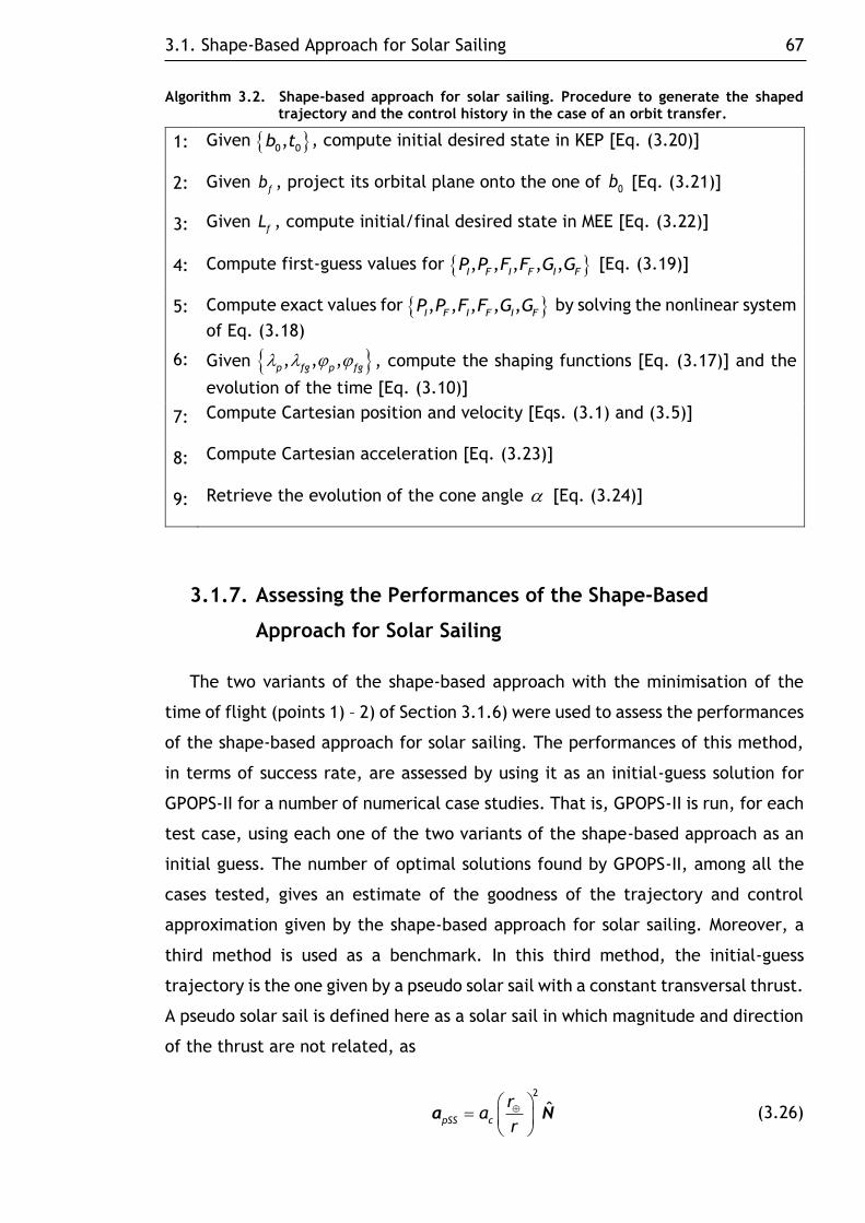
3.1. Shape-Based Approach for Solar Sailing 67
Algorithm 3.2. Shape-based approach for solar sailing. Procedure to generate the shaped trajectory and the control history in the case of an orbit transfer.
1: Given 0 0,b t , compute initial desired state in KEP [Eq. (3.20)]
2: Given f
b , project its orbital plane onto the one of 0b [Eq. (3.21)]
3: Given f
L , compute initial/final desired state in MEE [Eq. (3.22)]
4: Compute first-guess values for , , , , ,I F I F I F
P P F F G G [Eq. (3.19)]
5: Compute exact values for , , , , ,I F I F I F
P P F F G G by solving the nonlinear system
of Eq. (3.18)
6: Given , , ,p fg p fg , compute the shaping functions [Eq. (3.17)] and the
evolution of the time [Eq. (3.10)]
7: Compute Cartesian position and velocity [Eqs. (3.1) and (3.5)]
8: Compute Cartesian acceleration [Eq. (3.23)]
9: Retrieve the evolution of the cone angle [Eq. (3.24)]
3.1.7. Assessing the Performances of the Shape-Based
Approach for Solar Sailing
The two variants of the shape-based approach with the minimisation of the
time of flight (points 1) – 2) of Section 3.1.6) were used to assess the performances
of the shape-based approach for solar sailing. The performances of this method,
in terms of success rate, are assessed by using it as an initial-guess solution for
GPOPS-II for a number of numerical case studies. That is, GPOPS-II is run, for each
test case, using each one of the two variants of the shape-based approach as an
initial guess. The number of optimal solutions found by GPOPS-II, among all the
cases tested, gives an estimate of the goodness of the trajectory and control
approximation given by the shape-based approach for solar sailing. Moreover, a
third method is used as a benchmark. In this third method, the initial-guess
trajectory is the one given by a pseudo solar sail with a constant transversal thrust.
A pseudo solar sail is defined here as a solar sail in which magnitude and direction
of the thrust are not related, as
2
ˆpSS c
ra
ra N (3.26)

3.1. Shape-Based Approach for Solar Sailing 68
The trajectory starts at the initial set time and state and it is propagated for
a defined time of flight. In the orbital reference frame, the acceleration is
considered being always in the transversal direction, as
2
0 1 0T
pSS c
ra
ra (3.27)
The sign in Eq. (3.27) represents a thrust directed either towards or opposite
to the transversal unit vector and, therefore, an outward or inward spiral,
respectively. Note that a perfectly-reflecting flat solar sail cannot produce the
propulsive acceleration of Eq. (3.27) because the direction of such acceleration
would be defined by 2 , whereas its magnitude by 0 .
Regarding the numerical case studies, eleven single-leg rendezvous transfers
are considered in which the chosen objects are part of the PHA-NHATS database
used for the sequence-search phase (CHAPTER 4). Such database is made of PHAs
and asteroids part of the Near-Earth Object Human Space Flight Accessible Target
Study (NHATS) [206]. By definition, NHATS asteroids are targets possible to reach
from the Earth in a short (less than two years) return mission with low total
required v . PHAs, on the other hand, are in general characterised by higher v
if reached from the Earth. For this reason, all the transfers considered in this study
are so that the first object is either Earth or a NHATS asteroid and the second
object is a PHA.
Table 3.3 shows the main properties of the selected objects, whereas Table
3.4 details the properties of the transfers for each case study. Table 3.3 shows
that, among the chosen PHAs, seven are characterised by an eccentricity 0.2e
and seven are characterised by an inclination 2 degi . The departing date and
the time of flight for each rendezvous mission listed in Table 3.4 are taken from
the results of the search for sequences described in CHAPTER 4. The time of flight
is considered only if the transversal-thrust law is used as the initial guess. Both
inwards and outwards spirals are considered for the transversal-thrust law, as
shown in Eq. (3.27). Note that the ninth and tenth test cases study a transfer
between the same couple of asteroids but with different departing times and
times of flight (Table 3.4).

3.1. Shape-Based Approach for Solar Sailing 69
Table 3.3. Properties of the objects considered for the single-leg rendezvous missions.
Object , AUa e , degi PHA NHATS
Earth 1 0 0 no no
2011 CG2 1.178 0.158 2.757 yes yes
2005 TG50 0.923 0.135 2.402 no yes
2015 JF11 1.073 0.111 5.400 yes no
2012 KB4 1.093 0.061 6.328 no yes
2008 EV5 0.958 0.084 7.437 yes yes
2009 YF 0.936 0.121 1.523 no yes
2002 AW 1.071 0.256 0.571 yes no
2010 WR7 1.046 0.235 1.563 no yes
1989 UQ 0.915 0.265 1.299 yes no
2005 FG 1.122 0.213 3.882 no yes
1999 AQ10 0.934 0.236 6.501 yes no
2008 TX3 1.180 0.187 2.180 no yes
2000 EA14 1.117 0.202 3.555 yes no
2004 JN1 1.085 0.176 1.499 no yes
2006 KV89 1.150 0.273 3.554 yes no
2001 QE71 1.078 0.159 3.035 no yes
2001 US16 1.356 0.253 1.905 yes no
2015 EF7 1.209 0.225 3.570 no yes
2000 QK130 1.181 0.262 4.722 yes no
Table 3.4. Case studies for the single-leg rendezvous missions.
Case study Departing
object Arrival object
Departing
date
Time of
flight, days
1 Earth 2011 CG2 09 Jan 2029 690
2 2005 TG50 2015 JF11 26 Jan 2035 718
3 2012 KB4 2008 EV5 22 Feb 2031 647
4 2009 YF 2002 AW 23 Aug 2035 607
5 2010 WR7 1989 UQ 14 Jun 2024 640
6 2005 FG 1999 AQ10 19 Nov 2027 711
7 2008 TX3 2000 EA14 30 Aug 2028 740
8 2004 JN1 2006 KV89 31 Mar 2035 896
9 2001 QE71 2001 US16 06 Dec 2027 697
10 2001 QE71 2001 US16 23 Oct 2027 728
11 2015 EF7 2000 QK130 17 Apr 2026 531

3.1. Shape-Based Approach for Solar Sailing 70
An optimal solution to all the case studies shown in Table 3.4 has been sought
by using GPOPS-II with the three different initial guesses discussed above.
Moreover, the three NLP solvers available in GPOPS-II are used to test them in
problems like those ones discussed in this document. An optimisation is defined
successful when: a) the NLP solver returns a successful exit flag, b) a further mesh
refinement performed by GPOPS-II will not improve the quality of the solution,
and c) all the boundaries of time, state and control are verified through a post-
processing check. For the sake of conciseness, only the statistical results and the
control profiles of a representative case study are shown here. Table 3.5 shows
the number of successful cases for each initial guess used. On the other hand,
Table 3.6 shows the number of successful cases for each initial guess and each
NLP solver used. Figure 3.7a shows the control profile found by means of the
shaped-trajectory variant of the shape-based approach for case study 9. The
control profile of the optimised trajectory found by GPOPS-II with WORHP, for the
same case study, is shown in Fig. 3.7b.
Table 3.5. Number of successful cases for each initial guess.
Initial guess Number of successful cases
Transversal-thrust law 5/11 (45%)
Shape-based approach – propagated trajectory 10/11 (91%)
Shape-based approach – shaped trajectory 11/11 (100%)
Table 3.6. Number of successful cases for each initial guess and NLP solver.
Initial guess Number of successful cases
IPOPT SNOPT WORHP
Transversal-thrust law 3/11 (27%) 4/11 (36%) 4/11 (36%)
Shape-based approach
– propagated trajectory 9/11 (82%) 9/11 (82%) 9/11 (82%)
Shape-based approach
– shaped trajectory 9/11 (82%) 11/11 (100%) 11/11 (100%)
The overall results show that the use of the shape-based approach as an initial-
guess solution helps the convergence of GPOPS-II as ten optimal solutions have
been found out of the total number of eleven cases tested with the shape-based

3.1. Shape-Based Approach for Solar Sailing 71
guesses. In fact, an optimal solution has been found for all eleven cases tested
with the shaped-trajectory variant of the shape-based algorithm. On the contrary,
only five solutions have been found by using the trajectory obtained through the
transversal-thrust law as the initial guess. This validates the shape-based approach
developed for solar sailing. Moreover, the better performances shown by using the
shape-based approach against the transversal-thrust law endorse its use as an
initial guess for a high-fidelity direct-collocation optimisation method such as
GPOPS-II. The overall statistical results are very similar between the two variants
of the shape-based approach used, if no distinction among the NLP solvers is made
(Table 3.5). If the number of successful test cases is investigated as a function of
both the initial-guess method and the NLP solver used (Table 3.6), it can be seen
that, overall, the shaped-trajectory variant of the shape-based approach works
better than the propagated-trajectory variant. In fact, the statistical results show
a 100% success rate for both SNOPT and WORHP. Nevertheless, Table 3.6 shows
that both variants of the shape-based approach, as well as all the available NLP
solvers, are robust enough to be used in the early stages of solar-sail trajectory
design.
a) b)
Fig. 3.7. Shape-based approach (Case study 9). Control history found with (a) shape-based approach – shaped trajectory, and (b) GPOPS-II with NLP solver WORHP.

3.2. From Low Thrust to Solar Sailing: A Homotopic Approach 72
3.2. From Low Thrust to Solar Sailing: A Homotopic
Approach
An alternative method, with respect to the shape-based approach, has been
developed to quickly find preliminary solar-sail trajectories. The idea behind it is
to use a homotopic approach [64], together with a numerical continuation
technique [65], to find the desired solar-sail trajectory starting from a classical
low-thrust (LT) one. In fact, because of the differences in the control vector
between a classical LT propulsion system and a solar sail (Section 2.1.2), a low-
thrust OCP can be easier to solve numerically than a solar sail one.
The purpose of this section is to develop an efficient method to find a
minimum-time solar-sail transfer, starting from a solution for a low-thrust
minimum-time OCP, which can be easier to find or readily available. Given a
constant-mass low-thrust solution of the minimum-time OCP, the homotopic
transformation is introduced on the propulsive acceleration a . A constant-mass
LT is considered because the optimal control law for a LT-propelled spacecraft is
transformed to that of a propellantless solar sail. Moreover, finding a solution to
the minimum-time LT OCP with no mass variation is even easier than a classical
low-thrust OCP. As for the case of the shape-based approach for solar sailing
described in Section 3.1, the approximation of planar transfers is considered here.
Nevertheless, it has been demonstrated that, for small changes in the inclination,
the planar transfers obtained by means of this method are good approximations
of the 3D solar-sail solutions [66].
3.2.1. Mathematical Model
Consider a polar inertial reference frame ,r in the ecliptic plane, as shown
in Fig. 3.8. The state vector is
Tpol r u vx (3.28)
in which r is the radial distance of the spacecraft measured from the Sun,
identifies the spacecraft angular position from a fixed axis in space (inertial), u
and v are the radial and transversal spacecraft velocities, respectively. In this
case, the inertial axis, from which the angular position is computed, is the

3.2. From Low Thrust to Solar Sailing: A Homotopic Approach 73
direction of the vernal equinox (or first point of Aries) [203], as shown in Fig.
3.8. Therefore, note that can be actually related to the true longitude L .
However, will be used throughout this Section 3.2 to be consistent with the
common notation used for polar coordinates.
Fig. 3.8. Polar inertial reference frame in the ecliptic plane.
The equations of motion of a spacecraft under the action of gravity and a
generic acceleration a are [11]
2
2ˆ
ˆ
pol
u
v
r
v
r r
uv
r
a rx
a
(3.29)
Denoting with maxa the low-thrust maximum acceleration and with 0,1u
the non-dimensional control, the acceleration LTa given by a constant-mass low-
thrust system is
co,
s,
sinLT max
uaa (3.30)

3.2. From Low Thrust to Solar Sailing: A Homotopic Approach 74
The cone angle has the same meaning as in the solar-sail case, which is the
angle between the direction of the acceleration and the radial direction
( ˆcosLT
a r ). However, in the classical LT case, can assume any value, as
shown in Eq. (3.30). For the sake of clarity, recall the acceleration SSa given by a
solar sail as
2
2cos
cos ,s
,2 2in
SS c
ra
ra (3.31)
Optimal control problem formulation. The optimal control problems are
stated for both low-thrust and solar-sail cases [54]. The minimisation of the total
transfer time is considered for rendezvous (RV), flyby (FB), and orbit transfer (OT)
problems. Therefore, the objective function to be minimised is expressed as
0 0f f
J T t t (3.32)
From Eq. (3.32), it is clear that, in this case, the integral cost function is null
[see Eq. (2.25)]. Moreover, no path constraints are considered. Therefore, the
Hamiltonian defined in Eq. (2.26) becomes
T polxH (3.33)
in which the vector of the costates is defined as
T
r u v . The time
evolution of the costates is given by
T
polx
H (3.34)
The initial and final boundary conditions are derived for an orbit transfer, a
flyby and a rendezvous problem, as follows [11, 207].

3.2. From Low Thrust to Solar Sailing: A Homotopic Approach 75
00 0
1
f f
f
f f
f f
f
f
OT
OT
f
f
f
t
r t
t
u t
v t
t t
r
u
v
t
0
0
x x
xH
(3.35)
00 0
1
f f
f f
u f
f
f
f
B
f
FB
F
f
v
f
t
r t
t
t
t
t t
r
t
0
0
x x
xH
(3.36)
0 00
1
RV
RV
f
f f
f
f f
f
t
t
t tt
0
0
x x
x x
xH
(3.37)
The term 0x Eqs. (3.35) – (3.37) is the initial state of the departing object,
whereas the terms , , , ,f f f f f
r u vx are referred to the final state of the arrival
object. The last scalar boundary condition in Eqs. (3.36) – (3.37) is the
transversality condition on the Hamiltonian [Eq. (2.31)].
The optimal control laws for both low thrust and solar sail are derived by
minimising of the Hamiltonian with respect to the control variables. Consider the
first-order necessary condition for optimality and assume that no singular arcs
occur. That is, , 0,0u v
always. This hypothesis has been numerically
verified a posteriori for all the cases tested. Considering the Pontryagin’s
minimum principle, the optimal control law, in terms of the cone angle, is
argminH (3.38)

3.2. From Low Thrust to Solar Sailing: A Homotopic Approach 76
For the case of a constant-mass low-thrust system, the optimal control law is what
is usually referred to as a bang-bang thrust profile. That is, 1u and the
magnitude of the acceleration is the maximum available in all points of the
trajectory. The optimal direction of the thrust can be expressed, as a function of
the costates, as [102]
2 2 2 2
,cos sinu v
u v u v
(3.39)
in which , . On the other hand, for the case of a solar sail, Eq. (3.38)
becomes [2]
2 2
3 9 8tan
4
u u v
v
(3.40)
in which
2 2
, . It is worth noting that the optimal control law described
by Eq. (3.40) is defined for any values of ,u v
. In fact, it can be demonstrated
that
0
0limv
, if 0u
, and
0
l2
imv
, if 0u
.
3.2.2. Homotopy-Continuation Approach
In this section, the use of the homotopy to link the shooting functions relative
to the low-thrust and solar-sail OCPs is described. The shooting function for a
single OCP is represented by the nonlinear function : n mz , in which n
represents the number of optimisation variables and m is the number of nonlinear
scalar equations included in [208]. The zeros of the shooting function represent
the solution of the optimal control problem. For the OCPs at hand, such function
is expressed as
( )f
z (3.41)
in which z is the vector of the optimisation variables given by the initial values
of the costates 0t and the time of flight
0 fT , as follows.

3.2. From Low Thrust to Solar Sailing: A Homotopic Approach 77
0
0 fT
tz
(3.42)
Introducing the homotopic parameter 0,1 to link the solutions of the OCPs
throughout the homotopy, the shooting function becomes , : n mz .
When 0 , the shooting function is the one relative to the classical low-thrust
problem, whereas, when 1, the shooting function is the one relative to the
solar-sail problem.
Two linear homotopic transformations on the spacecraft acceleration are
considered and the related homotopic parameters are referred to as 1 and
2,
respectively. The first homotopic transformation is introduced as
2
2
1max 1
cos, ,1 co
s ns
iLTSS
ra u
ra a (3.43)
The corresponding shooting function is
1 1( , ) 0z (3.44)
The relation in Eq. (3.43) links the low-thrust acceleration of Eq. (3.30) to the one
that can be provided by a pseudo solar sail, given by Eq. (3.31) with maxc
a a .
Here, the term pseudo solar sail is referred to the fact that no constraint on the
thrust direction are enforced. That is, the pseudo-solar-sail solution of 1,1 0z
can be characterised by some points in the trajectory in which the acceleration is
directed towards the Sun. Nevertheless, such solution is used as initial guess for
the computation of the solar-sail OCP through a single-shooting approach. That is,
the zeros of 1,1 0z are computed subject to the constraint
,2 2
. In
all the numerical cases tested, the pseudo-solar-sail solution was always a good
initial guess for the direct computation of the solar-sail solution. Therefore, a
second homotopic transformation to link the solution of Eq. (3.44) with the solar-
sail OCP by continuously changing the boundaries on the cone angle, as shown in
[209], was not necessary.

3.2. From Low Thrust to Solar Sailing: A Homotopic Approach 78
The second linear homotopic transformation is introduced as the desired
characteristic acceleration can be different with respect to the corresponding
low-thrust acceleration (i.e. maxc
a a ). This second transformation allows linking
the initial solar-sail solution with ,0 maxc c
a a a to the final one, which is
characterised by max,fc c
a a a , as
2
2
2 ,0 2 ,
cos,1 cos ,
sin 2 2c c f
ra a
ra (3.45)
Note that the expression of the acceleration a in Eq. (3.45) is the same as the
one of a solar sail shown in Eq. (3.31), considering a modified characteristic
acceleration given by
2 ,0 2 ,
1c c c f
a a a (3.46)
In this case, the corresponding shooting function is
2 2( , ) 0z (3.47)
Numerical continuation. For both homotopies, which are described in terms
of the shooting functions of Eqs. (3.44) and (3.47), the zeros of the solar-sail
shooting function can be computed by using numerical continuation, starting from
the low-thrust solution LTz (Algorithm 3.3). This technique allows following the
so-called zero-path of the homotopy (i.e. the locus of solutions ( , )z of the system
( , ) 0z ) by numerically changing the parameter , starting from the solution
at 0 until computing the final solution at 1. The numerical continuation
used to solve the problem at hand is implemented in the form of discrete
continuation [208, 210]. That is, the value of the parameter is progressively
increased and, at each step, the solution of an intermediate OCP is computed.
Each intermediate solution is used as a starting point for the computation of the
following problem until the solution of the desired problem is found. The
continuation step size is determined as follows, starting by a defined initial value.
If the solution of an intermediate problem is found, the algorithm doubles the step
size to speed up the continuation process. On the contrary, if no solution is found

3.2. From Low Thrust to Solar Sailing: A Homotopic Approach 79
for the current intermediate problem, the step size is halved and the continuation
iteration is run again with a decreased step size until convergence is reached. If
the new step size is below a defined threshold min
, the algorithm terminates
unsuccessfully.
Algorithm 3.3. Homotopy-continuation approach.
1: Given 0 0,t b , compute
0
polx
2: Given 0 0
TT
LT LT ft Tz , initialise
LTz z
3: Define min max
,, , s.t.
4: While 1, Do
5: Solve , ,tmp
exitflag0z z
6: If 0exitflag , Then
7:
8: 2
9: If min , Then
10: Termination (Unsuccessful)
11: End If
12:
13: Else
14: Update tmp
z z
15: If 1, Then
16: 2
17:
18: Else
19: Termination (Successful)
20: End If
21: End If
22: End Do
Since the first homotopic transformation shown in Eq. (3.43) introduces some
complexity in the OCP formulation discussed in Section 3.2.1, a close look at the
transformed OCP formulation is given in the following subsection. On the contrary,
the second homotopic transformation does not affect the OCP formulation, being
the homotopy related to the value of the characteristic acceleration only.

3.2. From Low Thrust to Solar Sailing: A Homotopic Approach 80
Transformed optimal control problem formulation. The equations of motion
that describe the evolution in time of the state of the spacecraft during the first
homotopy are
m
2
2
1 1ax2
2
1
0
0co
cos
s
sin
pol
LTSS
u
v
r ra uv
rr r
uv
r
x (3.48)
The part of the Hamiltonian that depends only on the control variables u and
is denoted by H and expressed as
3 2sin cos cos sin cosT
LTSSA B C DaH (3.49)
in which
max max
2 2
max max
1 1
1 1
(1 ) , (1 )
,
v u
u v
ua ua
r ra a
r r
A B
C D (3.50)
Accordingly, the time evolution of the costates, shown in Eq. (3.34), becomes
2 3 2 22
2 3 3 2 3
1 1
2
2 cos 2 cos sin2
0
1 2
c cr u v
u r v
v v u
a r a rv uv v
r r r r r r
v
r
u v
r r r
(3.51)

3.2. From Low Thrust to Solar Sailing: A Homotopic Approach 81
The first-order optimality condition, shown in Eq. (3.38), becomes
6 5 4
3 2
( ) 2( 3 ) ( 11 )
4( 3 ) ( 11 ) 2( 3 ) ( ) 0
A D B C A D
B C A D B C A D
H (3.52)
in which
tan2
, thus 12tan ( ) . On the hypothesis that no singular arcs
occur, the first-order optimality condition for u leads to
1 if 0
0 i
cos sin
cos sif n 0
u v
u v
u (3.53)
It should be noted that no analytical solution exists for the roots of the sixth-order
polynomial of Eq. (3.52), in the generic case in which both 0u and 0
v .
Therefore, the optimal control can be only found by means of a numerical
algorithm able to compute the optimal values *u and * that minimise H . That
is, for each value of the non-dimensional control u in Eq. (3.53), the real roots of
the sixth-order polynomial of Eq. (3.52) are numerically computed. Therefore, the
value of H is evaluated for all the sets of solutions ,u , retrieving the optimal
control as
, argmin ,u uH (3.54)
3.2.3. Numerical Test Cases
In this section, four numerical test cases are presented (Table 3.7). The first
two test cases are considered to validate the proposed approach. As such, two
planar circular-to-circular Earth-Mars orbit transfers are studied with different
values of the sail characteristic acceleration. In these cases, the proposed
homotopic approach is compared with both a conventional solution method, which
is based on the use of a metaheuristic algorithm, and the results found in the
literature. The last two test cases are considered to assess the performances of
the proposed method in computing a solution to a planar rendezvous OCP. As such,
two planar rendezvous transfers from Earth to asteroid (99942) Apophis are
considered with different values of the sail characteristic acceleration. In these

3.2. From Low Thrust to Solar Sailing: A Homotopic Approach 82
last two test cases, the results found by means of the proposed homotopic
approach are compared with those ones shown in [211].
Table 3.7. Homotopic approach: numerical test cases.
2, mm sc
a Problem
Test case 1 1 Earth-Mars orbit transfer
Test case 2 0.1 Earth-Mars orbit transfer
Test case 3 0.6 Earth-Apophis rendezvous
Test case 4 0.12 Earth-Apophis rendezvous
Table 3.8 shows the main properties, in terms of Keplerian elements, of both
Mars and Apophis. Apophis orbit is considered coplanar with the ecliptic plane.
This assumption is reasonable in a first approximation, being its inclination only
3.3 deg [66]. The Earth orbit is considered circular with radius 1 AUr .
Table 3.8. Homotopic approach: Keplerian elements of the target objects on 14 Feb 2016. The inclination of both objects is assumed equal to zero.
Object , AUa e , degi , deg , deg , deg
Mars1 1.52368 (0) (0) (0) (0) (0)
(99942) Apophis2 0.92228 0.191 (0) 204.5 126.4 283.4
The tolerances on the errors on the final state have been set to 1,000 km, for
the position, and 0.1 m s , for both the radial and transversal velocities, as stated
in [11]. These tolerances are the same for all the test cases considered in this
section. It is also worth mentioning that a C++ implementation of the Bulirsch-
Stoer algorithm has been used to propagate the equations of motion more
efficiently, with higher accuracy and lower computational effort than the
conventional ordinary differential equation (ODE) solvers [212]. The absolute and
relative tolerances for the propagator have both been set to 810 [11]. All the
simulations have been performed in MATLAB on a 3.4 GHz Core i7-3770 with 16 GB
1 The orbit of Mars is assumed planar and circular. Moreover, only the semimajor axis is
considered, being Mars used only for orbit-transfer problems. The value of the semimajor axis is the same as the one considered in [11].
2 Data available online at https://cneos.jpl.nasa.gov/orbits/elements.html [retrieved 08 August 2015].

3.2. From Low Thrust to Solar Sailing: A Homotopic Approach 83
of RAM, running Linux Ubuntu 14.04. In the next subsections, the four test cases
are discussed in detail.
Validation of the homotopic approach: Earth-Mars orbit transfer. The first
two test cases have been considered for the purpose of (a) validating the novel
method proposed for computing solar-sail OCPs and (b) comparing its
performances with respect to a conventional GA method used to solve the same
solar-sail OCPs. The objective function to be minimised within the GA is the
Euclidean L2 norm of the shooting function (1( ,1)z or
2( ,1)z , according to the
specific test case).
Twenty different sets of settings have been considered for the GA simulations,
differing in the population size (Population = 50,100,150,200,500 ) and the
maximum number of generations allowed (MaxGenerations =
500,1000,1500,2000 ). Because of the heuristic nature of the GA, each set of
settings has been run 100 times and statistical values have been considered for
the comparison. Moreover, the solutions from GA have been refined by means of
a gradient-based method, which is implemented in the interior-point algorithm in
the MATLAB function fmincon. The results for GA are expressed in terms of success
rate of each set of settings, which is the percentage of runs (out of 100) that
terminate with at least one feasible solution (a solution within the required
tolerances). It has been noted that GA showed improved performances (in terms
of both computational time and success rate) if the transversality condition (which
is the last scalar boundary condition in Eqs. (3.35) – (3.37)) was not considered.
From an analytical point of view, it can be demonstrated that the transversality
condition is negligible, at least for what concerns the problems at hand [66, 102,
103]. For these reasons and for the sake of consistency, the transversality
condition on the Hamiltonian has been excluded in all the numerical cases
considered throughout this section. Nevertheless, it has been verified a posteriori
that the transversality condition was always verified. Because of the
transversality-condition avoidance, Eqs. (3.44) and (3.47) reduce to an
underdetermined system of nonlinear equations. That is, a least-square numerical
solver [213] is needed to find the solutions of such system within the homotopic
approach. However, it has been empirically verified that this approach is both

3.2. From Low Thrust to Solar Sailing: A Homotopic Approach 84
numerically stable and faster than (or, at least, as fast as) solving a square system,
at least for the cases tested.
The first test case is the planar circular-to-circular Earth-Mars orbit transfer
described in [11]. The low-thrust maximum acceleration has been considered the
same as the characteristic acceleration in the reference paper. That is,
2
max1 mm s
ca a . The results of both the homotopy approach and the GA are
shown in Table 3.9. The first row of Table 3.9 shows the number of sets with a
success rate above 90% (note that the homotopy can only be either successful or
not successful, since it is a deterministic approach). For the GA, the computational
time is the lowest average computational time among all the sets of settings with
a success rate above 90%. In Table 3.9, the minimum and maximum values of the
time of flight are shown for the GA. The result obtained through the homotopy
approach is consistent with those obtained via the GA method. Moreover, the
result found by means of the homotopic approach is in perfect agreement with
what shown in [11] (i.e. 0
407.7 daysf
T ). Only eight sets of settings of the GA
out of twenty have a success rate above 90% and the homotopy method is 42%
faster than the GA.
Table 3.9. Homotopic approach: homotopy and GA results comparison (Test case 1).
Homotopy GA
Sets with success rate above 90% - 8/20
Computational time, s 11 19
0, days
fT 407.72
407.69 (min)
407.72 (max)
Figure 3.9a shows the evolution of the cone angle over time during the first
continuation, which is from low thrust (green thick dashed line) to pseudo solar
sail (red thick continuous line), as shown in Eq. (3.43). All the intermediate
solutions are represented by thin cyan lines. Figure 3.9b shows the comparison
between the low-thrust (green dashed line) and the solar-sail (red continuous line)
cone angle over time. Figures 3.10a and 3.10b show the low-thrust and solar-sail
transfer trajectories, respectively. A plot of the acceleration vector along the
transfer is also shown. Figure 3.11a shows the zero-path of the homotopy, as

3.2. From Low Thrust to Solar Sailing: A Homotopic Approach 85
defined in [201], whereas Fig. 3.11b shows the evolution of the continuation
parameter during the first continuation.
a) b)
Fig. 3.9. Homotopic approach (Test case 1). Control history for coplanar circular-to-circular Earth-Mars orbit transfer (ac = 1 mm/s2). (a) Cone angle evolution during first continuation. (b) Low-thrust and solar-sail cone angle evolution.
a) b)
Fig. 3.10. Homotopic approach (Test case 1). Ecliptic plane view of the transfer trajectories for coplanar circular-to-circular Earth-Mars orbit transfer (ac = 1 mm/s2). (a) Low thrust. (b) Solar sail.
a) b)
Fig. 3.11. Homotopic approach (Test case 1). (a) Zero-path. (b) Evolution of .

3.2. From Low Thrust to Solar Sailing: A Homotopic Approach 86
A second scenario has been tested, considering the same problem but with a
smaller solar-sail characteristic acceleration (i.e. 20.1 mm sc
a ). That is, the
second continuation, described in Eq. (3.45), can be applied to the solution of the
previous test case. On the other hand, the optimisations through GA shall be
repeated with the new value of the characteristic acceleration. Table 3.10 shows
the comparison between the results of the homotopy approach and GA. The
computational time shown for the homotopic approach is the one needed to find
a solution to the second continuation only, starting from the solution of the first
one found in the previous test case. Note that this scenario is purely of academic
interest. In fact, it is unlikely that anybody would ever launch a seven-year solar-
sail mission to Mars. Nevertheless, this scenario is a good test bed for the second
continuation, given the long flight time.
Table 3.10. Homotopic approach: homotopy and GA results comparison (Test case 2).
Homotopy GA
Sets with success rate above 90% - 14/20
Computational time, s 1 16
0, days
fT 2661.51
2661.34 (min)
2661.43 (max)
Figure 3.12a shows the evolution of the cone angle during the second
continuation, in which the characteristic acceleration changes from
2
,01 mm s
ca to 2
,0.1 mm s
fca . Figure 3.12b shows the planar circular-to-
circular Earth-Mars orbit-transfer trajectory through a solar sail with
20.1 mm sc
a . As for Test case 1, the plots of the zero-path of the homotopy
and the evolution of the continuation parameter are shown in Fig. 3.13. In this
case, the continuation parameter needs to be halved several times when the
solution of the intermediate problem is not found, as described in Algorithm 3.3.
Nonetheless, despite the larger number of continuation steps with respect to Test
case 1, the convergence of the algorithm is very fast, as shown in Table 3.10.

3.2. From Low Thrust to Solar Sailing: A Homotopic Approach 87
a) b)
Fig. 3.12. Homotopic approach (Test case 2). Coplanar circular-to-circular Earth-Mars orbit transfer (ac = 0.1 mm/s2). (a) Cone angle evolution. (b) Solar-sail transfer trajectory (ecliptic plane view).
a) b)
Fig. 3.13. Homotopic approach (Test case 2). (a) Zero-path. (b) Evolution of .
Validation of the homotopic approach: Earth-Apophis rendezvous. The last
two test cases aim to validate the proposed approach for more complex transfer
scenarios. While keeping the hypothesis of planar transfers, the homotopic
approach is now applied to solar-sail optimal transfers to rendezvous with an
object onto an elliptic orbit. As shown in Table 3.7, the mission scenario consists
in a solar-sail transfer from the Earth to rendezvous with the asteroid (99942)
Apophis, as described in [211].
The spacecraft is injected directly into an interplanetary trajectory at Earth,
with zero hyperbolic excess energy, on 27 July 2017, as in [211]. The only
difference between the two cases tested is the value of the characteristic
acceleration. In Test case 3, the value of the characteristic acceleration is

3.2. From Low Thrust to Solar Sailing: A Homotopic Approach 88
20.6 mm sc
a , which corresponds to a sail lightness number 0.1, whereas,
in Test case 4, 20.12 mm sc
a , which corresponds to 0.02 [Eq. (2.20)]. The
two values correspond to the extreme values in the range of the sail lightness
numbers considered in [211], for a solar-sail-only transfer. The initial solution of
the low-thrust Earth-Apophis rendezvous OCP is computed by means of the PSO
algorithm described in Appendix B.2, in the Hamiltonian formulation. The
maximum acceleration considered for the low-thrust solution is 2
max0.6 mm s .a
Therefore, the first homotopy is used to find a solar-sail solution with
20.6 mm sc
a (Test case 3). Such solution is subsequently used to find the solar-
sail trajectory for Test case 4. The results of the two numerical cases presented
in this section are summarised in Table 3.11, together with the results shown in
[211]. As already discussed for Test case 2, the computational time shown in Table
3.11 and related to Test case 4 is the one needed for the second continuation
only, since the solution of the solar-sail OCP with 20.6 mm sc
a was already
found in Test case 3.
Table 3.11. Optimal solar-sail rendezvous from Earth to (99942) Apophis (in brackets the values from [211]).
Test case 3 Test case 4
2, mm sc
a 0.6 0.12
Computational time, s 28 1
0, days
fT 457 (468) 1160 (1260)
Figure 3.14 shows the optimal solar-sail transfer trajectories for both
20.6 mm sc
a and 20.12 mm sc
a . Figure 3.15 shows the evolution of the cone
angle during the second continuation. As shown in Table 3.11, the results are in
good agreement with the ones presented in [211], considering that those solutions
are computed for 3D transfers rather than planar transfers. Nevertheless, it has
been shown that the planar solutions presented here can be used as first-guess
solutions for a single-shooting approach to easily compute 3D transfers [66].
Furthermore, despite an increased complexity of the OCP to be solved, both Test
cases 3 and 4 require a little computational time, comparable with the ones of
the previous test cases, relative to circular-to-circular orbit transfers.

3.2. From Low Thrust to Solar Sailing: A Homotopic Approach 89
a) b)
Fig. 3.14. Homotopic approach (Test cases 3 and 4). Ecliptic plane view of the solar-sail transfer trajectories for rendezvous from Earth to (99942) Apophis. (a) ac = 0.6 mm/s2. (b) ac = 0.12 mm/s2.
Fig. 3.15. Homotopic approach (Test case 4). Cone angle evolution during the second continuation.
The proposed homotopic approach allows computing optimal solar-sail
trajectories for a wide range of characteristic accelerations, in a single and fast
run. This is achieved by means of the continuation on the characteristic
acceleration, in which intermediate solutions with
,0 ,,
cc c fa a a are computed
at each successful iteration. Other approaches would usually require a single
optimisation to be performed for each value of the characteristic acceleration,
leading to a higher computational effort to obtain the entire family of solutions.
Therefore, the homotopic approach presented here is particularly appealing for
preliminary mission design. In fact, the early stages of a solar-sail mission planning
are usually characterised by an uncertainty on the value of the sail characteristic

3.2. From Low Thrust to Solar Sailing: A Homotopic Approach 90
acceleration. For instance, in [16], the value of the characteristic acceleration is
shown as a function of the sail size for the DLR/ESA Gossamer Roadmap. A
preliminary mission is described in [16] which considers a characteristic
acceleration 20.3 mm sc
a and a sail size in the range between 2
54 m and
2
65 m , depending on the bus mass taken into account. One of the improvements
outlined in [16] is to find a solar-sail trajectory, within the same mission criteria,
with a lower value of the characteristic acceleration. For instance, Fig. 3.16 shows
a plot for the minimum time of flight 0 f
T as function of ca (computed by means
of the second homotopic continuation) in the case of the Earth-Apophis planar
rendezvous with characteristic acceleration bounded in 20.12,0.6 mm s
ca . A
time of flight of about 660 days is needed if a sail with a characteristic
acceleration 20.3 mm sc
a is considered.
Fig. 3.16. Minimum time of flight as a function of the characteristic acceleration for the coplanar Earth-Apophis case.

3.3. Discussion 91
3.3. Discussion
In this chapter, two different formulations for a fast solar-sail trajectory design
have been presented in the coplanar approximation: the shape-based approach
and the homotopic approach. The two formulations are conceptually very
different. In fact, in the case of the shape-based approach, the trajectory is
designed by means of predefined shaping functions and the control is analytically
retrieved a posteriori. Since there is no explicit control on the acceleration
history, a genetic algorithm is used to find the shape of the trajectory that best
fits the acceleration feasible by the given spacecraft. The use of the genetic
algorithm within the shape-based approach slightly slows down the overall method
but allows a more automatic use of the method. In fact, the inputs required from
the user are minimal. On the other hand, the homotopic approach exploits the
Pontryagin’s minimum principle to find the (locally) optimal solution to the given
solar-sail optimal control problem. This approach has been shown to be very
accurate and fast. Moreover, the output of this method is already an optimal
solution to the desired coplanar transfer. The drawback of this approach lies in
the sensitivity of the indirect method. In fact, even though the use of the
homotopy increases the convergence radius of the indirect method, the initial
values of the continuation parameter and its initial step size, as well as the
maximum and minimum allowed step size, may still affect the convergence of the
solution. Furthermore, the proposed method does not consider the computation
of the low-thrust solution. That is, the effort needed to find such solution should
be taken into account if an actual comparison between the computational efforts
of the two presented approaches is required. On the contrary, the shape-based
approach is a standalone method that does not need any pre-computed initial
guess to start with.
Because of the advantages and drawbacks of both methods, each approach is
used for a different purpose, as it will be shown in the next chapters. The shape-
based approach is used when several preliminary solar-sail trajectories are
needed, exploiting the little input needed from the user. On the contrary, the
homotopic approach is used in the cases of more complex mission scenarios that
do not require a large number of trajectories to be found.

CHAPTER 4.
ASTEROID SEQUENCE SEARCH
This chapter describes the developed approach to find a set of sequences of
asteroids for a multiple-NEA rendezvous mission through solar sailing. Finding a
sequence of NEA to be visited is primarily a combinatorial problem because of the
large amount of objects and the huge number of possible permutations between
them, as pointed out in Section 4.1. Furthermore, for each transfer leg, an
optimisation problem must be solved to assess the existence of a trajectory
feasible by a solar sail. For these reasons, two subsets of the whole NEA database
are introduced to reduce the amount of objects to deal with, as explained in detail
in Section 4.1. Therefore, the sequence search algorithm, described in Section
4.4, is characterised by a local pruning to reduce further the number of NEAs to
test in each step of the tree-search algorithm, as detailed in Section 4.2. Lastly,
the shape-based approach for solar sailing, described in Section 3.1, is used to
have a reliable approximation of the solar-sail trajectory within a reasonable
amount of time.
The content of this chapter was published in [198, 214-216], except for Test
cases 2-4 in Section 4.6.1.

4.1. Asteroid Database Selection 93
4.1. Asteroid Database Selection
The choice of target asteroids to be visited in a mission is a difficult task
because it shall consider, among all, composition, scientific interest, orbital
dynamics, and available launch window. NASA’s Near Earth Object Program listed
12,840 NEAs on 08 August 20151 and this number is rapidly increasing. All those
objects with an Earth minimum orbit intersection distance (EMOID) 0.05 AU and
an absolute magnitude 22 (i.e. diameter 110 240 m , depending on the
albedo2) are classified as PHAs. The problem of finding a sequence of encounters
is firstly a combinatorial problem. In fact, more than a trillion of sequences of
three objects can be found, if all the possible combinations with permutations are
considered. Moreover, there seem to be no clear common priorities on the
selection of NEAs in the scientific community. To reduce this huge amount of
possible combinations, further classifications can be considered which consider
the interest from an exploration point of view. Barbee et al. [206] introduced the
Near-Earth Object Human Space Flight Accessible Target Study (NHATS) in which
the objects are selected as those for which a four-impulse return mission can be
found within a set of design parameters such as total v required, total mission
duration, stay time at the object, and launch date interval. Because the mission
parameters for the trajectory computation can be set in several different ways,
the list of NHATS asteroids is not univocally defined.
To have a more useful and interesting database, a subset containing only PHAs
and NHATS asteroids is, therefore, considered in this work. This database contains
1,801 objects, 1,607 of which are PHAs. The criteria used to select the NHATS
database are the following.
1 Data available online at https://cneos.jpl.nasa.gov/orbits/elements.html [retrieved 08 August
2015].
2 Data available online at http://www.minorplanetcenter.net/iau/lists/Sizes.html [retrieved 08 August 2015].

4.1. Asteroid Database Selection 94
total required 8 km s
total mission duration 450 days
stay time at the object 8 daysNHATS criteria:
launch : 2015 2040
absolute magnitude 26
OCC 7
v
(4.1)
The term OCC in Eq. (4.1) is the Orbit Condition Code of a NEA’s orbit, which
refers to the accuracy of the orbit determination. For a complete explanation of
the above criteria, the interested reader is referred to the JPL/NASA NHATS
website1. In the following, this subset will be referred to as the PHA-NHATS
database.
Boden et al. [159] studied the target selection for manned NEA exploration and
realised that the NEA accessibility to date is limited due to uncertainties in the
objects’ characterisation and the available technology. Nonetheless, they pointed
out, “there might be more targets within the currently known NEA population” for
a NEA sample return mission. “One reason is that the actual rotation rates of most
NEAs are unknown”. A fast rotator, in fact, is not suitable for a sample return
mission, either human or robotic. On the other hand, slow rotators can exist
among those asteroids for which there currently is little knowledge about the
rotation. Therefore, a second subset for a multiple NEA rendezvous mission can
consider those objects with a large uncertainty on the rotation rate to improve
our knowledge for better planning a future exploration mission. The asteroid
lightcurve database (LCDB) is “a set of files generated from a database that
includes information directly and indirectly obtained from observations made to
determine the period and/or amplitude of asteroid lightcurves” [217]. The quality
code U provides the assessment of the quality of the period solutions within the
LCDB. For this reason, a second subset is considered in this study, which considers
PHAs and those NEAs in the LCDB with 2U . That is, all those objects for which
the given value of the rotation rate is not reliable for a statistical analysis. Such
second database contains 1,813 objects, 271 of which are NEAs in the LCDB with
2U 2. Note that, as for the PHA-NHATS database, all the 1,607 known PHAs are
1 Data available online at https://cneos.jpl.nasa.gov/nhats/intro.html [retrieved 08 August
2015].
2 Data available online at http://www.minorplanet.info/lightcurvedatabase.html [retrieved 20 February 2016].

4.1. Asteroid Database Selection 95
also considered as part of this second database. In the following, this subset will
be referred to as the PHA-LCDB database.
Table 4.1 shows the characteristics of the two databases considered in this
work.
Table 4.1. Characteristics of the two reduced databases considered.
Database PHAs NHATS LCDB Total
PHA-NHATS database 1,607 204 8 1,801
PHA-LCDB database 1,607 8 271 1,813
A graphical comparison between the complete database and the PHA-NHATS
database is given in Fig. 4.1, in which the heliocentric positions of all objects are
plotted for both databases, at a given reference time.
Fig. 4.1. Heliocentric view of the positions of all known NEAs (small blue dots) and PHAs (large red dots) on 24 March 2017. (a) Complete database. (b) PHA-NHATS database. Bodies not to scale.
It is worth noting that the two subsets considered in this study are very
different from each other. Despite the fact of having a similar number of objects
and being made mostly of PHAs, the PHA-NHATS database contains NHATS
asteroids that are, by definition, easy to be reached from the Earth. Therefore,
their orbital elements do not differ much from those of the Earth. In contrast,
there is not such constraint on the LCDB objects considered in the PHA-LCDB

4.1. Asteroid Database Selection 96
database. Such difference between the two databases can be visualised as follows.
Define the Tisserand parameter related to the Earth as [218]
212 cos
a erT i
a r (4.2)
in which the orbit of the Earth is considered circular. Perozzi et al. [169] proposed
the use of the Tisserand parameter related to the Earth as an indication of the
relative unperturbed velocity of an asteroid at close encounter with the Earth. To
do so, the parameter is defined as
3 T (4.3)
The negative value of the inverse normalised semimajor axis
r a can be plotted
against 2 . Figure 4.2 shows the distribution of all NEAs in the complete database
in the 2, r a space. The Earth in such space is in the point 0, 1 . The dashed
blue line has been obtained setting to zero both inclination and eccentricity in the
computation of the Tisserand parameter, thus representing the circular limit of
an orbit with the given value of the semimajor axis. That is, the portion of space
on the left side of the circular limit represents a forbidden portion of space, being
characterised by 2 0e . The Earth tangency condition is also plotted as a magenta
solid line. It has been obtained setting to zero the inclination in Eq. (4.2). Such
condition represents an orbit with a given semimajor axis being tangent with that
of the Earth. Except for the trivial case in which the unknown orbit is exactly that
of the Earth, the only other case in which the tangency condition is verified is
when either the radius of pericentre p
r or the radius of the apocentre ar is equal
to the semimajor axis of the Earth. This condition univocally defines the geometry
of the orbit on the ecliptic plane, as follows.
1 if
1 if p
ar r a e a r
r r a e a r (4.4)
1 if
1 if
re a r
a
re a r
a
(4.5)

4.1. Asteroid Database Selection 97
Substituting Eq. (4.5) into Eq. (4.2) and considering 0i , the expression of 2
for the tangency condition is given by
tangencycondition
2 3 2 2r r
a a (4.6)
Note that all the NEAs in the complete database have 0.5 AUa and, therefore,
Eq. (4.6) is defined for all the objects in the database. The distance along the 2
axis of a NEA from the tangency condition provides an indication of the additional
velocity needed for a planar rendezvous with the selected object. Such velocity
should be added to the one needed for the apocentre/pericentre manoeuvre once
the tangency condition is reached. Moreover, the quantity
r a on the y-axis is
related to the asteroid orbital energy normalised with respect to that of the Earth.
From Fig. 4.2, it is clear that the NHATS asteroids are easier to reach from the
Earth, since their energy is close to the one of the Earth 1.2, 0.8r a
and 2 0.1. On the other hand, the NEAs from LCDB with 2U are spread
over the allowed 2, r a space. Therefore, finding feasible sequences of
asteroids within the PHA-LCDB database is expected to be more difficult.
Fig. 4.2. Distribution of all NEAs in the (𝚼2, -r⨁/a) space. The two curves represent the circular limit and the Earth tangency condition.

4.1. Asteroid Database Selection 98
From a purely combinatorial point of view, an order of magnitude for the
complexity of the problem of finding a sequence of encounters can be given by
considering the total number of possible sequences of 3, 4 and 5Q objects
without repetition, both from the original and the two reduced databases. The
number of these Q -permutations of N objects N
QP (Table 4.2) is given by
!
!
N
Q
NP
N Q (4.7)
Table 4.2. Number of Q-permutations of N objects within the complete database and the reduced ones.
Database N 3Q 4Q 5Q
Complete database 12,840 122.1 10 162.7 10 203.5 10
PHA-NHATS database 1,801 95.8 10 131.0 10 161.9 10
PHA-LCDB database 1,813 95.9 10 131.1 10 161.9 10
Such combinatorial problem can be easily visualised for the specific case of an
asteroid sequence search. If all the objects in the considered database are used,
the asteroid sequence search can be represented as a tree, as discussed in Section
2.2.6 and schematically shown in Fig. 4.3. The BS implementation of the tree
search is considered in this work (see Section 2.2.6). The implementation of BS
has been chosen against DFS because it allows considering a maximum fixed
number of partial sequences as starting point for the next leg. A drawback of this
method is that complete sequences are available only at the end of the tree
search. On the other hand, the DFS implementation allows having complete
sequences already at the early stages of the tree-search run. However, branching
criteria based on the quality of the sequences found cannot be defined in the DFS
implementation. Figure 4.3 shows how the computational effort needed to find
all the possible branches in the tree grows as more feasible transfers are found.
The dotted red lines in the figure represent branches of the tree for which no
feasible solution has been found. In order to reduce further the computational
cost of the asteroid sequence search, a local pruning on the database is carried
out at the beginning of each leg. A detailed description of it is given in the next
Section 4.2.

4.2. Local Pruning on the Database 99
Fig. 4.3. Schematic of the tree search.
4.2. Local Pruning on the Database
A local pruning on the available NEA database is performed, based on
astrodynamics. This has been carried out to work on a locally reduced database,
for the reasons mentioned in Section 4.1. The local pruning is performed at the
beginning of each leg of the sequence and it depends on the starting orbit of the
respective leg, as it will be discussed in detail in Section 4.4.
Four conditions for the local pruning of the database are used: the first three
criteria are related to the in-plane trajectory, whereas the fourth takes into
account the orientation of the orbital planes:
i. The current spacecraft state is propagated, in an outward and inward
spiral, for the maximum allowed time of flight 0 ,maxf
T considered within
the trajectory model. A control law that maximises the semimajor axis
change is considered for the propagation of the spacecraft state. To obtain
the maximum and minimum semimajor axes, the locally-optimal law for
changing the semimajor axis through solar sailing, described in [2], is
used. The optimal sail cone and clock angles can be expressed as
1
1 1
if tan 1/ 2
tan 1/ 2 if tan 1/ 2
0
(4.8)
N objects to testK1 feasible trajectories
K1*(N-1) objects to testK2 feasible trajectories
K2*(N-2) objects to testK3 feasible trajectories
Earth
First leg
Second leg
Third leg

4.2. Local Pruning on the Database 100
in which
23 9 8tantan
4tan (4.9)
The angle in Eq. (4.9) represents the cone angle relative to the ideal
direction of the thrust for the maximisation of the change of the desired
orbital element. For the maximisation of the semimajor axis, such angle
has the following expression [2]:
1 costan
sin
e
e (4.10)
The maximum and minimum semimajor axes obtained are, then, the
maximum and minimum semimajor axes that the solar sail can reach
starting from the current state and traveling for the maximum available
time of flight. All NEAs with a semimajor axis outside the available range
are therefore excluded from the locally pruned database for the current
leg.
ii. Similarly to the preceding case, the trajectory is propagated by
considering a control law that maximises the change of eccentricity and
thus a maximum range of possible eccentricity variation is found. Only
those NEAs with eccentricity inside the available range are included in the
locally pruned database for the current leg. As in the preceding case, the
optimal sail cone and clock angles are given by Eqs. (4.8) – (4.9). However,
in this case, the angle is given by the following relation [2]:
2 cos cosectan cot
1 cos 1 cos
e e
e e (4.11)
iii. Defining the longitude of pericentre as , a transfer trajectory
between two orbits (subscript 1 and 2) with a large 1 2
m d ,o
is more difficult to achieve as the eccentricities of the two orbits increase.
This can be verified with the following test cases, in which two 200-day
transfers are computed by means of a zero-full-revolution ballistic
Lambert arc [77, 170, 219]. Keplerian elements of departing and arrival

4.2. Local Pruning on the Database 101
orbits are the same in both cases except for the eccentricity, as shown in
the following.
0
TEST CASE 1
1 AU 0.1 0 0 0 0
1 AU 0.1 0 30 deg 0 180 deg
Tkep
Tkep
f
x
x
(4.12)
0
TEST CASE 2
1 AU 0.5 0 0 0 0
1 AU 0.5 0 30 deg 0 180 deg
Tkep
Tkep
f
x
x
(4.13)
Figure 4.4 shows the Lambert solution for both transfer trajectories. The
difference in the required v is highlighted in the figure: the required
v related to the second test case is more than three times larger than
that of the first test case.
For this reason, a threshold on the maximum variation of the longitude of
pericentre has been considered for each object, taking into account the
value of the eccentricity as follows.
2
max1 e (4.14)
By using this threshold, the arrival object is removed from the locally-
pruned database if at least one of the following conditions is not satisfied.
1 max,1 2 max,2
2 max,2 1 max,1
mod mod
mod
,2 ,2
,2 d ,2mo (4.15)
In Fig. 4.5, two examples (not to scale) are sketched to give a graphical
view of the pruning on the longitude of pericentre given by Eq. (4.15).
Figure 4.5a shows a case in which Eq. (4.15) is satisfied and, in fact, the
ranges of possible variation of for the two objects overlap. On the other
hand, in Fig. 4.5b, the orbit of the second object is more eccentric, so
that the available range of variation of is smaller and does not overlap
with the one of the first object. In this second case, the first condition in
Eq. (4.15) is not satisfied and the second object is, therefore, not part of
the locally pruned database for the current leg.
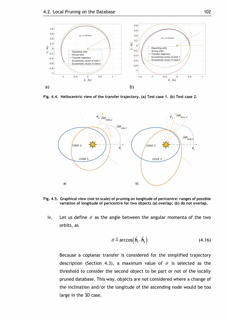
4.2. Local Pruning on the Database 102
a) b)
Fig. 4.4. Heliocentric view of the transfer trajectory. (a) Test case 1. (b) Test case 2.
Fig. 4.5. Graphical view (not to scale) of pruning on longitude of pericentre: ranges of possible variation of longitude of pericentre for two objects (a) overlap; (b) do not overlap.
iv. Let us define as the angle between the angular momenta of the two
orbits, as
1 2
ˆarccos hh (4.16)
Because a coplanar transfer is considered for the simplified trajectory
description (Section 4.3), a maximum value of is selected as the
threshold to consider the second object to be part or not of the locally
pruned database. This way, objects are not considered where a change of
the inclination and/or the longitude of the ascending node would be too
large in the 3D case.

4.3. Simplified Trajectory Model 103
4.3. Simplified Trajectory Model
A simplified trajectory model is used to check the feasibility of the trajectory
transfer from each object of the current leg to all the others in the locally pruned
database. One possibility is to use a ballistic Lambert-arc approximation, in which
the acceleration needed for the transfer is compared to the maximum
acceleration that the solar sail can achieve, multiplied by a penalty factor1.
However, a low-thrust trajectory differs from a ballistic Lambert arc and this
difference increases with the time of flight. Furthermore, a solar sail performs
best for trajectories with long flight times, due to the low but continuous
acceleration. In order to obtain solutions that are more reliable from the sequence
search and, therefore, decrease effort and time needed in the optimisation phase,
the shape-based approach described in Section 3.1 has been used with the
objective function 0 f
J T . In fact, the timeline of the asteroid encounters is one
of the fundamental output of the asteroid sequence search. The relative phasing
between two consecutive encounters at the beginning of the transfer trajectory
and the available transfer time are two essential characteristics of the sequence
that can affect the feasibility of the overall multiple rendezvous mission. That is,
it may be difficult to find a solar-sail solution for a sequence of asteroids and
encounter dates found by means of the ballistic Lambert-arc approximation. On
the other hand, the shape-based approach gives a better description of the
trajectory. Therefore, the output of the asteroid sequence search (i.e. the
sequence of asteroids and encounter epochs, which will be referred to as timed
sequence) is more likely to describe a mission feasible by a solar sail if the shape-
based approach is used. The drawback of the shape-based approach, with respect
to the use of Lambert arcs, is the use of the genetic algorithm that increases the
computational time needed to find preliminary sequences. Nevertheless, the
increased complexity of the transformation of Lambert arcs into solar-sail
trajectories and, therefore, the little reliability of such trajectory model, with
respect to solar sailing, justifies the increased computational time needed by the
shape-based approach. Other methods are used in the literature for guessing the
1 Peloni, A. and Ceriotti, M., “Solar Sailing Multiple NEO Rendezvous Mission: Preliminary
Results”, First Stardust Global Virtual Workshop (SGVW-1) on Asteroids and Space Debris, University of Strathclyde, Glasgow, Scotland, UK, 6-9 May 2014. Presentation available online at https://www.youtube.com/watch?v=j-uxCvo09Hc [retrieved 06 June 2017].

4.4. Sequence Search Algorithm 104
v needed for a low-thrust transfer which exploit, for instance, Edelbaum’s
formulation [220] or a parametrisation of the trajectory [59]. These would be
faster than the shape-based approach if used within the sequence search.
However, as for the case of the Lambert-arc approximation, these methods do not
consider the dynamics of a solar sail, which is more constrained than that of a
classical low thrust. Lastly, a low-v transfer is sought for classical low-thrust
trajectories because of the limited amount of propellant onboard. For solar
sailing, however, the amount of v is not a good indicator for the feasibility of a
transfer trajectory.
4.4. Sequence Search Algorithm
Figure 4.6 shows the flowchart of the process of searching for sequences, which
is detailed in Algorithm 4.1. First, the selected database (i.e. the PHA-NHATS or
the PHA-LCDB database, in this case) is locally pruned (details in Section 4.2) by
taking into account that the sequence starts at Earth at a fixed time 0t . This
pruning allows the algorithm to consider a list of encounters ,b tmp
L that contains
fewer objects at a time, avoiding spending time on objects that would be difficult
to reach. Approximated solar-sail trajectories are found by means of the shape-
based approach, as discussed in Section 4.3. For all the trajectories found, the
arrival NEAs are kept and considered as starting objects for the next iteration of
the algorithm. This is carried out by updating the list part
L that contains all the
partial timed sequences found so far. Next, once the objects in the current pruned
list ,b tmp
L have been considered for the trajectory calculation, the same process is
carried out in a tree-search algorithm, starting from the arrival body of each of
the temporary timed sequences is found so far. When the total mission duration
reaches the maximum allowed time (i.e. ten years, in the current scenario) or no
feasible solar-sail trajectories are found, the current timed sequence is
considered complete. Once all the temporary timed sequences are completed and
the list of partial timed sequences is empty (i.e. part
L ), the algorithm stops.
The computational time of the described sequence search increases as the
number of feasible transfer trajectories increases due to the tree nature of the
search itself (Fig. 4.3). Therefore, the possibility to reduce the number of partial

4.4. Sequence Search Algorithm 105
timed sequences considered at the beginning of each leg is added. Define max
seqN as
the maximum number of partial timed sequences to be used in the following leg
within the sequence search algorithm. Once all the potential transfer trajectories
have been studied for the current leg, the set tmp
L of all the partial timed
sequences found is rearranged so that these are sorted in ascending order with
respect to the total mission time. This is done so that those timed sequences with
fastest transfers have higher priority, since one of the goals of the sequence
search is to find sequences with as many encounters as possible within a fixed
mission time. Therefore, only the first max
seqN timed sequences that are part of tmp
L
are used for the next leg of the tree search. The discarded timed sequences are
stored so that they can be used or analysed after the algorithm has stopped.
Note that the only stochastic component of the sequence search algorithm is
the GA used within the shape-based approach. Except this, the algorithm is fully
deterministic.
The code has been implemented using mixed MATLAB/C code, speeding up the
computations where bottlenecks have been found in the MATLAB code (Appendix
B.1). Moreover, the algorithm is parallelised for different launch dates, since each
run assesses one specific launch date (Algorithm 4.1, Line 1).
Fig. 4.6. Sequence search flowchart.
Complete selected database
Local pruning on Keplerian elements
Semi-analytical approximated trajectory (coplanar shape-based method) to all available NEAs
Timed sequence complete
Mission time < 10 years?YES
NO
At least one trajectory satisfies the accelerations
requirements?
YES
NO
Add stay time at the object

4.4. Sequence Search Algorithm 106
Algorithm 4.1. Sequence search algorithm.
1: Given 0 0,t b , initialise 0 0
T
partL t b
2: Local pruning on ,b b tmp
L L
3: For each object ,j b tmp
b L , Do
4: Check the existence of a solar-sail trajectory 0f
T
5: If a feasible trajectory exists, Then
6:
0 0 0 0f f stay
parpar t
j j
t
t T t T tL L
b b
7: End If
8: End For
9: compl
L
10: While part
L , Do
11: For each partial timed sequence is , Do
12: Retrieve the last time of the timed sequence: 1,endi
t s
13: Retrieve the list of the bodies already encountered: ,
2,allb i i
L s
14: ,
\b b b i
L L L
15: Local pruning on ,b b tmp
L L
16: For each object ,j b tmp
b L , Do
17: Check the existence of a solar-sail trajectory 0f
T
18: If a feasible trajectory exists, Then
19:
0 0f f stay
tmp part
j j
t T t T tL L
b b
20: End If
21: End For
22: If tmp
L , Then
23: compl compl i
L L s
24: End If
25: End For
26: ;part tmp tmp
L L L
27: End While

4.5. Application to Gossamer Mission 107
4.5. Application to Gossamer Mission
The reference work of Dachwald et al. [16] showed a three-NEA rendezvous
mission through solar sailing, considering a sailcraft with a characteristic
acceleration 20.3 mm sc
a and a maximum mission duration of ten years. The
sequence of encounters, according to the DLR/ESA Gossamer roadmap [16], should
be made of at least three NEAs with a stay time in the order of a few days. The
mission lifetime should be at most ten years. Moreover, the mission should respect
the following criteria:
a) At least one object should be a PHA.
b) At least one object should be a potential target for future human
exploration (i.e. it should be part of the temporary NHATS database).
c) The last NEA should be a small object (i.e. absolute magnitude 25.5 ).
Note that the reason for the last point was to demonstrate the feasibility of a solar
sail as a gravity tractor [221, 222]. However, this point is not considered one of
the main aims of such a mission but rather a secondary goal1. Therefore, a
sequence of NEAs that satisfies the first two criteria but is characterised by the
last object being larger than 50 m in diameter is still considered a good sequence.
Because of the nature of the sequence search algorithm described in Section
4.4, these criteria can only be verified a posteriori. Although there is no guarantee
for meeting the above requirements, a large number of sequences are discovered.
Therefore, the candidate sequences are chosen such to best fit criteria a) – c) and
that are made of the largest number of encounters.
Moreover, Dachwald et al. [16] proposed three further steps to be investigated
in future works for improving the technical feasibility and for increasing the
support of the scientific and planetary defence communities:
i) Reduction of the total mission duration.
ii) Reduction of the required characteristic acceleration.
iii) Priority on PHAs within the target selection.
A reduction in the total mission duration has not been explicitly considered in
the current work. Nevertheless, within the asteroid sequence search, the timed
sequences are sorted for total mission duration and, if the maximum allowed
number of temporary sequences is exceeded, those with the longest mission
1 Prof Bernd Dachwald, 03 October 2014. Personal communication.

4.6. Numerical Test Cases 108
duration are discarded. Moreover, sequences with more than three encounters
have been found for the same maximum mission duration, as it will be shown in
Section 4.6.
A reduction of the required characteristic acceleration was addressed by
considering a solar sail with a characteristic acceleration
20.1, 0.15, 0.2 mm sc
a . Some results for the sequence search considering
20.3 mm sc
a will be shown as well for the sake of comparison. It is worth to
underline that, in the ideal case of a perfectly-reflecting flat solar sail, the
characteristic acceleration depends only on the area-to-mass ratio (AMR), as
shown in Eq. (2.19). Therefore, a characteristic acceleration 20.2 mm sc
a ,
instead of 20.3 mm sc
a , leads to a reduction of the AMR from 233 m kg to
222 m kg . That is, either more payload is allowed on the same sail or the use of
a smaller sail or a heavier structure is considered, with the result of lowering the
technological challenges and thus increasing the mission-specific TRL of the
available technology. According to the DLR/ESA Gossamer technology [3], such a
reduction in the characteristic acceleration leads to a reduction in the sail size
from about 2 2
54 m - 65 m to about 2 2
39 m - 48 m . The interval of sail
dimensions depends on the sailcraft bus adopted, as discussed in [16].
Finally, the solutions with at least one PHA are preferred to the others in the
final sequence selection.
4.6. Numerical Test Cases
The methodology proposed has been applied to the two reduced databases
described in Section 0. In the following subsections, the results of the sequence
search for both databases are shown and discussed.
4.6.1. PHA-NHATS Database
The PHA-NHATS database introduced in Section 4.1 is used for the first set of
test cases. Therefore, the output sequences are very likely to fulfil the
requirements from the DLR/ESA Gossamer roadmap, as discussed in Section 4.5.

4.6. Numerical Test Cases 109
Starting from the departure date of the reference mission (which is
0
28 November 2019t ), a systematic search of sequences has been carried out
on a set of launch dates spanning about ten years with a step size of 90 days
028 November 2019, 06 October 2029t . This choice allows taking into
account short- and long-term variations in the phasing between the asteroids. The
four values of the sail characteristic acceleration discussed in Section 4.5 are
considered to test different scenarios (namely, Test case 1 – 4, respectively). The
characteristics of each test case are shown in Table 4.3. Moreover, the minimum
allowed time of flight for each leg is the same in all test cases and is set to
0 ,min
500 daysf
T . The number of preliminary sequences found for each value of
the characteristic acceleration can be an indicator of the performances needed
by a solar sail for this kind of mission. In the following subsections, the four cases
tested are discussed and the results are shown.
Table 4.3. PHA-NHATS database: test cases for the sequence search algorithm.
2, mm sc
a 0 ,max, days
fT , days
stayt
max
seqN
Test case 1 0.20 1,000 100 ∞
Test case 2 0.15 1,500 50 ∞
Test case 3 0.10 1,500 50 ∞
Test case 4 0.30 1,000 100 200
Test case 1. For this test case, the pruning on the maximum number of
considered sequences is not limited and, therefore, it is max
seqN in Table 4.3.
This search resulted in more than 4,800 unique sequences made of five
encounters, of which at least one is a PHA. It is important to underline that all
the sequences found within this study contain only NHATS asteroids and sometimes
a PHA. Figure 4.7 shows the number of unique sequences found for each launch
date. Here, the term unique sequence refers to the sequence of asteroids only,
without considering the possible differences in time. Only those sequences with
at least one PHA and at least four encounters are plotted. Note that more than
400 unique sequences with five encounters and at least one PHA have been found
for a single launch date (which is 0
t 14 April 2028). If sequences with more than

4.6. Numerical Test Cases 110
four encounters and at least one PHA are considered, more than 1,000 unique
sequences have been found for a single launch date (which is 0
t 09 January
2029).
Fig. 4.7. Number of unique sequences with at least one PHA and four encounters as a function of the launch date. PHA-NHATS database with ac = 0.2 mm/s2 (Test case 1).
Figure 4.8 shows an example of the first three legs of all the timed sequences
with five encounters and at least a PHA found for the launch date 0
t 30 April
2025. The graph shows the typical tree nature of the solution, as discussed in
Section 0. Two different timed sequences are considered having a rendezvous with
the same object when the arrival times differ by 40 days at most. For example,
the object 2012 BB4 appears three times in the second leg but the rendezvous
times differ by more than 100 days. Therefore, these are considered as three
separate branches of the solution tree. The sequence characterised by the dashed
red path (that is, the sequence Earth – 2000 SG344 – 2015 JD3 – 2012 KB4) is the first
one of the fully-optimised sequences that will be shown in Section 5.4.3.
Figure 4.8 shows how several timed sequences are partly repeated. This allows
the target asteroids to be easily changed, even after launch, if needed. Moreover,

4.6. Numerical Test Cases 111
because a solar sail does not need any propellant, such a change is theoretically
easier with a solar sail than with an electric propulsion system.
Because of the tree nature of the sequence search and the need of a GA run to
check the existence of each trajectory, the whole search has been carried out by
running several parallel searches for the 41 launch dates over three different
machines: a 3.4 GHz Core i7-3770, a 3.4 GHz Core i7-4770, and a 2.3 GHz Core
AMD Opteron 6376. The first two machines have 16 GB of RAM and run Windows
7. The third one is part of the University of Glasgow Computer Cluster Facility1,
has up to 8 GB of RAM per core and runs CentOS 6. Considering only those
simulations carried out on the latter, which is the slowest machine, the average
computational time for each sequence search run is about 41.3 days, where each
successful run of the shape-based approach took about 60 seconds on average.
1 Data available online at http://www.gla.ac.uk/services/it/hpcc/ [retrieved 24 August 2015].

4.6. Numerical Test Cases 112
Fig. 4.8. Tree graph of first three legs of all timed sequences with five encounters found for launch date t0 = 30 April 2025 (Test case 1).

4.6. Numerical Test Cases 113
Test case 2. For this test case, a maximum allowed time of flight
0 ,max
1,500 daysf
T has been considered within the trajectory model to account
for the lower performances of the sailcraft. Such increased upper boundary on the
allowed flight time potentially reduces the number of objects that can be visited
by the chosen sailcraft within the maximum mission duration limit of ten years. In
fact, if the stay time at each object (Algorithm 4.1) used in the previous test case
is considered and the duration of each transfer leg is set to 0 ,maxf
T , only two
objects can be visited in ten years, as follows:
0 ,max 0 ,max 0 ,min
3,200 days 10 yearsf stay sf ftay
T t T t T (4.17)
However, if the stay time at each object is reduced to 50 daysstay
t , the
possibility to visit a third object with a shorter time of flight is added, as follows:
0 ,max 0 ,max 0 ,min
3,600 daysstay sf f tay f
T t T t T (4.18)
This is the reason for considering a stay time 50 daysstay
t for this test case, as
shown in Table 4.3. Nonetheless, the results are expected to show sequences
made of fewer objects with respect to the previous Test case 1. In fact, Fig. 4.9
shows that no sequences with five encounters are found. Nevertheless, this search
resulted in more than 1,200 unique sequences made of four encounters, of which
one is a PHA. If sequences with more than three encounters and at least one PHA
are considered, more than 3,200 unique sequences have been found over the ten-
year time span considered. That is, these results show that a large number of
three-NEA rendezvous missions still exists if a sailcraft with a characteristic
acceleration that is half of the one in the reference paper [16] is considered. In
fact, more than 40 unique three-NEA sequences exist for each launch date
considered.

4.6. Numerical Test Cases 114
Fig. 4.9. Number of unique sequences with at least one PHA and three encounters as a function of the launch date. PHA-NHATS database with ac = 0.15 mm/s2 (Test case 2).
Fig. 4.10. Number of unique sequences with at least one PHA and three encounters as a function of the launch date. PHA-NHATS database with ac = 0.1 mm/s2 (Test case 3).

4.6. Numerical Test Cases 115
Test case 3. For this test case, the values of the maximum allowed time of
flight and the stay time are chosen for the same reasons explained in the previous
subsection for Test case 2. Figure 4.10 shows the results for this test case. In this
case, the sail characteristic acceleration is too low to guarantee a significant
number of sequences made of at least two NEAs and a PHA for each launch date
considered. In fact, there are no such sequences for certain launch dates.
Test case 4. This case has been studied to show the potential amount of
sequences feasible if the characteristic acceleration of the DLR/ESA Gossamer
roadmap is considered [16, 51, 52]. Moreover, because of the larger characteristic
acceleration with respect to the previous test cases, a large amount of sequences
is expected to be found. For these reasons, as well as to decrease the total
computational time required, a reduced set of launch dates has been considered
for Test case 4. Moreover, the algorithm for this test case has been set so that
max
200seqN . That is, only the 200 timed sequences with the shortest time of flight
are kept for the next leg. This significantly reduces the amount of sequences that
will be found. Nevertheless, this search resulted in yet an extremely large number
of feasible sequences. In fact, considering both the complete and the discarded
(and thus incomplete) sequences, more than 20,000 unique sequences made of at
least five encounters, of which one is a PHA, are found. Figure 4.11 shows the
number of unique sequences found for each launch date. Only those sequences
with one PHA and at least five encounters are plotted. Note that more than 600
unique sequences with at least five encounters and one PHA have been found for
each launch date considered. Moreover, more than 1,000 sequences with six
encounters in less than ten years have been found as well. In fact, Fig. 4.11 shows
that there are up to 229 unique sequences made of six NEAs, of which one is a
PHA, for a single launch date (which is 0
t 26 May 2020).

4.6. Numerical Test Cases 116
Fig. 4.11. Number of unique sequences with at least one PHA and five encounters as a function of the launch date. PHA-NHATS database with ac = 0.3 mm/s2 (Test case 4).
Note the peak of sequences found for 0 0
t t 26 May 2020 (Fig. 4.11). An
analysis of it might give an insight about the structure of the solution itself. Among
the 2,188 sequences found for this launch date, 1,240 are characterised by the
first two ordered encounters being 2011 CG2 and 2014 UN114. That is, more than
half of the branches of the solution tree grow from the same bough. If the next
depth of the tree is analysed, it can be seen that more than half of the solutions
develop over three branches only. Figure 4.12 shows the first three depths of the
solution tree for 0
t . Specifically, it is shown that 1,490 sequences share the same
first encounter, whereas only 698 sequences are characterised by a different one.
The results found for 0
t 11 May 2023, which is the launch date relative to the
second peak shown in Fig. 4.11, are qualitatively similar. In fact, the two NEAs
2011 CG2 and 2014 UN114 are again the two most recurrent objects in all the
sequences found for that very launch date. In particular, 2011 CG2 is the second
encounter after 2012 BB14 for about 400 sequences. On the contrary, among all
the 1,039 unique sequences found for the first launch date (Fig. 4.11), 2011 CG2
appears only 108 times in total.

4.6. Numerical Test Cases 117
Fig. 4.12. Tree graph of the first three legs of all sequences with five encounters found for launch date t0 = 26 May 2020 (Test case 4). The number of sequences that share the same branch is shown above each of them.
Further analysis is carried out on 0
t to study the repeatability of the solution.
Specifically, two more runs of the sequence search are performed for
0 0
2 dayst t . The run for 0 0
2 dayst t resulted in 1,949 unique sequences
found with at least five encounters, one of which is a PHA. This is compatible with
what found for 0 0
t t . On the other hand, only 817 unique sequences were found
for 0 0
2 dayst t which is a significantly smaller number. An analysis on the
characteristics on the last run shows that there are no sequences for which the
first two ordered encounters are 2011 CG2 and 2014 UN114. This explains the
difference in the total number of sequences found. However, it is unlikely that a
difference of two days in the launch date causes the loss of the phasing between
the Earth and the two NEAs. Therefore, six runs of the sequence search are
performed for the same launch date to investigate the repeatability of such
solution. The results are shown in Fig. 4.13. It can be seen that five runs out of
six resulted into a number of unique sequences comparable with that of 0 0
t t
shown in Fig. 4.11. In fact, the result of the second run is the only one in which
no sequences are characterised by the first two encountered being 2011 CG2 and
2014 UN114. A deeper analysis shows that the leg from the Earth to 2011 CG2 for
the second run takes 956 days. On the contrary, all the other runs, for which the
leg from 2011 CG2 to 2014 UN114 is found, show a time of flight for the first leg of

4.6. Numerical Test Cases 118
about 537 days. This means that two minima exist in the OCP solved by GA. If GA
finds the local minimum 0
956 daysf
T , the phasing between 2011 CG2 and 2014
UN114 is lost and no solution exists. Note that this holds true for the problem
formulation considered. It can be shown that a feasible solar-sail trajectory does
indeed exist with 0
=1,200 daysf
T between the two objects. It is worth reminding,
however, that the maximum allowed time of flight has been chosen as
0 ,max
1,000 daysf
T in the current study (Table 4.3).
The discussion above highlighted an intrinsic characteristic of the tree search.
That is, a whole set of solutions might not be shown in the results of the sequence
search if no solutions are found for one branch or this is discarded by the BS
algorithm. For instance, it has been shown that several local minima (within the
chosen problem formulation) exist for one single leg. By using the genetic
algorithm, there is a statistical confidence that the global minimum is found but
there are rare cases in which this does not happen. In these cases, all the branches
that grow from those legs will be affected. Nonetheless, the results of the
sequence search showed that more than 600 unique sequences are found for each
launch date. Therefore, there is a guarantee that at least the preliminary
sequences shown exist.
Lastly, from the results shown for this test case, it can be seen that the choice
of sorting the partial sequences in ascending order with respect to the total
mission duration produced good results, in terms of number of sequences with at
least one PHA. Therefore, there is no need to add an explicit rule that analyses
the objects in each partial sequence. If, however, one wants to weight more those
sequences that already contain one or more objects of interest (e.g. PHAs), a
different rule can be considered for ordering the sequences to keep for the next
leg. A Pareto optimality rule, for instance, could be used to sort the partial
sequences so that preference is given to those sequences with the shortest mission
time and the largest number of PHAs.

4.6. Numerical Test Cases 119
Fig. 4.13. Number of unique sequences with at least one PHA and five encounters for six runs on the sequence search for launch date t0 = 28 May 2020 (Test case 4).
4.6.2. PHA-LCDB Database
The PHA-LCDB database introduced in Section 4.1 has been chosen to test the
reliability of the proposed approach on a more challenging mission scenario than
transfers between NHATS asteroids. Because of this, the number of sequences
found by the sequence search algorithm is expected to be significantly smaller
than what found considering the PHA-NHATS database.
For this test case, only one value of the characteristic acceleration is
considered. That is, 20.2 mm sc
a . The same set of departure dates considered
in the case of the PHA-NHATS database and discussed in Section 4.6.1 is used in
this case. A stay time of 50 days has been considered between two consecutive
legs within the sequence search algorithm. A maximum time of flight of 1,000 days
for each leg was allowed in the sequence search with the PHA-NHATS database,
whereas a maximum one-leg time of flight of 1,500 days was chosen for this study.
This choice has been driven by the fact that the single transfers are more
challenging in the case of the PHA-LCDB database.

4.7. Discussion 120
This search resulted in 589 unique sequences made of three encounters, of
which at least one is a PHA. Figure 4.14 shows the number of unique sequences
found for each departure date. Only those sequences with at least one PHA and
at least three encounters are plotted.
Fig. 4.14. Number of unique sequences with at least one PHA and three encounters as a function of the launch date. PHA-LCDB database with ac = 0.2 mm/s2.
4.7. Discussion
In this chapter, a methodology to find sequences of encounters for multiple
NEA rendezvous missions through solar sailing was presented and discussed. The
sequence search algorithm is characterised by: (a) the use of the shape-based
approach, presented in CHAPTER 3, to find approximated solar-sail trajectories,
(b) a local pruning to reduce the computational effort needed, and (c) the use of
two reduced databases of objects. Moreover, the proposed sequence search
algorithm returns sequences of NEAs with preliminary epochs for the asteroid
encounters, i.e. timed sequences. This provides a guideline for the next phase of

4.7. Discussion 121
the mission design, which is the trajectory-optimisation phase, as it will be
discussed in CHAPTER 5.
The use of the PHA-NHATS database resulted in more than 4,800 unique
sequences made of at least five asteroids (at least four NHATS asteroids and at
least one PHA) within less than ten years of total mission duration. This is true if
a solar sail with lower performances than the one considered in a previous
reference study is taken into account. If, instead, the characteristic acceleration
of the reference work is used, it has been shown that an extremely large number
of feasible sequences of at least five NEAs, of which one is a PHA, does exist.
However, a reduction of the characteristic acceleration was one of the future
steps to be addressed in the DLR/ESA Gossamer roadmap, as a lower characteristic
acceleration involves a smaller or heavier sail for the same spacecraft bus.
Therefore, this study showed that the mission-related TRL for the available solar-
sail technology is larger than it was previously thought and that such a mission can
be performed with current or at least near-term solar sail technology1. Moreover,
it was shown that, at least for the PHA-NHATS database, a 5-NEA-rendezvous
mission is always possible within ten years by means of a solar sail.
The PHA-LCDB database was used to test the proposed asteroid sequence
search on a different scenario. In fact, this second study was characterised by
transfers that are more challenging than those of the previous study, which
considered NHATS objects that, by definition, are targets easy to reach from the
Earth.
An additional advantage of the proposed sequence search algorithm is the
generation of a set of several feasible timed sequences, rather than a single
optimal one. This is of great help to the mission analysts or the decision makers
in the choice of the best mission. In fact, a solution is defined optimal on the basis
of the mathematical model and mission parameters (e.g. launch window, current
objects of interest, etc.) considered. If there is a change in one of these
parameters within a later phase of the mission design, the single “optimal”
solution, which has been found in a preliminary mission design phase, can be
worthless.
1 Note that a sail characteristic acceleration ac = 0.2 mm/s2 is within the capability of current
and near-term Gossamer sailcraft technology, according to [16, 31, 223]. Moreover, the technology developed at DLR for a controlled deployment of a Gossamer spacecraft is currently on TRL four approaching level five, according to [50].

4.7. Discussion 122
Finally, this study showed that, for each launch date, hundreds of accessible
NEA target sequences exist even within the restricted database of targets.
Therefore, it can be concluded that there are little to no constraints on the launch
window for a multiple-NEA rendezvous mission, if a solar sail is involved.
Moreover, solar sailing has the advantage of flexibility on the target asteroids.
The targets do not have to be selected before launch and they can be changed en
route if, for instance, scientific or commercial interest changes over the years of
the mission or when a new target of particular interest appears.

CHAPTER 5.
SEQUENCE OPTIMISATION
Once complete sequences of encounters for a multiple NEA rendezvous mission
through solar sailing have been found, an optimisation problem must be solved to
find 3D solar-sail trajectories. This chapter describes two optimisation approaches
developed for finding multiple NEA rendezvous trajectories feasible by a solar sail.
Both approaches employ the general-purpose optimal control software GPOPS-II,
which uses a variable-order adaptive Radau collocation method, together with
sparse nonlinear programming, as discussed in Section 2.2.2.
Several numerical test cases are shown and discussed to: (a) test the reliability
of the proposed algorithms, (b) test such algorithms in an environment
characterised by minimal inputs from the user, and (c) demonstrate the
capabilities and the versatility of the solar-sail propulsion system.
The content of this chapter was published and/or presented in [31, 197-200,
214-216].
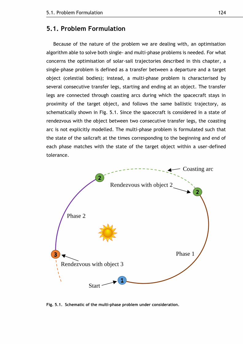
5.1. Problem Formulation 124
5.1. Problem Formulation
Because of the nature of the problem we are dealing with, an optimisation
algorithm able to solve both single- and multi-phase problems is needed. For what
concerns the optimisation of solar-sail trajectories described in this chapter, a
single-phase problem is defined as a transfer between a departure and a target
object (celestial bodies); instead, a multi-phase problem is characterised by
several consecutive transfer legs, starting and ending at an object. The transfer
legs are connected through coasting arcs during which the spacecraft stays in
proximity of the target object, and follows the same ballistic trajectory, as
schematically shown in Fig. 5.1. Since the spacecraft is considered in a state of
rendezvous with the object between two consecutive transfer legs, the coasting
arc is not explicitly modelled. The multi-phase problem is formulated such that
the state of the sailcraft at the times corresponding to the beginning and end of
each phase matches with the state of the target object within a user-defined
tolerance.
Fig. 5.1. Schematic of the multi-phase problem under consideration.
Phase 1
Phase 2
Rendezvous with object 2
Rendezvous with object 3
Start
Coasting arc

5.1. Problem Formulation 125
The dynamics within each phase is defined, in modified equinoctial elements,
as [7]
Ax x a b x (5.1)
in which a is the propulsive acceleration given by Eq. (2.18). The terms A x and
b x that appear in Eq. (5.1) are, respectively, the matrix and vector of the
dynamics expressed, in the orbital reference frame ˆ, ,r h , as follows [7]:
2
2
20 0
1sin 1 cos sin cos
1cos 1 sin sin cos
cos0 0
2
sin0 0
2
10 0 sin cos
p p
q
p p p gL q L f h L k L
q q
p p p fL q L g h L k L
q q
p s L
q
p s L
q
ph L k L
q
A x (5.2)
2
0 0 0 0 0
T
qp
pb x (5.3)
The terms q and 2s are the auxiliary variables defined in Eq. (3.3). Note that
both the state x and the acceleration a in Eqs. (5.1) - (5.3) are functions of the
time but their explicit dependency on the time has been omitted for the sake of
readability.
The problem of finding the optimal control vector
r h
T
N N Nu such
that the total mission duration is minimised while fulfilling the dynamics
constraints of Eq. (5.1) at any time, is solved via a direct collocation method [88].
This has been chosen against indirect methods because:

5.1. Problem Formulation 126
1. It is easier to deal with multi-phase problems. Furthermore, if the number
of phases is not fixed, the problem should be reformulated each time the
number of phases varies, if an indirect approach is used.
2. Its convergence to an optimal solution is usually easier than with an
indirect method, although the solution is less accurate. Nevertheless, very
accurate solutions are not required at this stage of the mission design.
3. Finding first guesses for the costates needed in the indirect method is
usually difficult, since the costates do not have any physical meaning. On
the other hand, an initial guess for the trajectory and the control history
is usually easier to find.
The control vector u should be bounded so that 1, 1,
hN N , whereas
0, 1r
N because of the inability of the solar sail to thrust towards the Sun.
Moreover, a path constraint should be considered which enforces the control
vector to be a unit vector. However, it has been noted that the NLP solvers can
sometimes have difficulties in solving an OCP for which the optimal control lies
exactly on the bounds. This is more likely to happen if a path constraint is set
which enforces the magnitude of the control vector to be within certain limits1.
Therefore, the bounds on each component of the control vector are set to be
larger than one and no path constraint on the magnitude of the control vector is
enforced. Nevertheless, the actual thrust unit vector considered within the
dynamics is the normalised control vector, such as
ˆ uN
u (5.4)
In this way, there is one less constraint to be satisfied and the problem is
numerically easier to solve. Note that the components of the normal unit vector
are preferred to the sail clock and cone angles as a control vector. Because of
their periodicity, in fact, the sail control angles can lead to numerical issues within
direct optimisation methods. Additionally, a set of endpoint constraints must be
satisfied in each phase j , such as
1 Dr Anil V. Rao, February 2016. Personal communication.

5.2. STO: Sequential Trajectory Optimiser 127
0 max
0 max
,
,
j j
f
j j
f
t t r
t t v
r
v (5.5)
in which r and v are, respectively, the position and velocity error of the
spacecraft with respect to the target.
Lastly, and again to help the numerical convergence of the optimiser, the
problem is scaled so that 1r and 1. Because all the considered target orbits
are near the Earth, this scaling guarantees that the norm of the position vector is
always 1r ; a characteristic acceleration 20.2 mm sc
a is scaled to
0.0337c
a in normalised units. Note that 1510c
a r if the SI units are
used, whereas the scaled problem is so that 210c
a r , which is more
suitable for numerical optimisation.
5.2. STO: Sequential Trajectory Optimiser
The sequential trajectory optimiser (STO) is the first optimisation approach
developed to find solutions to the multiple NEA rendezvous mission problem. The
trajectory found through the coplanar shape-based approach described in Section
3.1 is used as an initial-guess solution for the optimiser, which transforms it into
a 3D trajectory. The general-purpose optimal control software GPOPS-II, together
with the NLP solver SNOPT [72], is used within STO. Note that the interface for
WORHP within GPOPS-II was not yet implemented at the time STO was developed
and this is the reason for which WORHP has not been used within STO.
An algorithm has been developed in MATLAB to find the optimal trajectory in
terms of total mission duration, as shown in Fig. 5.2. Given the selected timed
sequence (i.e. list of target objects and encounter epochs), the algorithm
performs as follows.
1) The algorithm automatically computes the initial guess for each leg
separately by means of the shape-based approach with the objective
function of Eq. (3.25), as described in Section 3.1.6. To avoid possible
numerical problems in the optimisation phase that can affect the
convergence of the optimiser, several initial-guess solutions are generated

5.2. STO: Sequential Trajectory Optimiser 128
for each leg. That is, the trajectory is propagated by considering both a
constant control law between two points of the shaped function and a
cubic spline interpolation of the control law. Moreover, two different
stopping criteria are considered in the GA, so that four different initial-
guess solutions are generated for each leg.
2) The algorithm optimises the 3D trajectory leg by leg. Each initial guess is
optimised both without considering any further scaling method and by
further scaling the problem through the automatic-guessUpdate choice
provided by GPOPS-II [89]. Moreover, if no feasible or optimal solutions
are found for the current leg, the default hp adaptive mesh refinement is
changed so that the one developed by Liu et al. [92] is used for the whole
optimisation. Within this optimisation phase, the solution of each leg is
constrained to start at least two days after the arrival of the previous leg.
In this way, the optimiser is forced to find a solution that guarantees a
minimum time in the vicinity of the object for close-up observations.
Moreover, a multi-phase optimisation, which would only be used to reduce
the total mission duration, is not necessary.
3) Finally, if at least one feasible solution is found in all the legs individually,
the whole multi-phase trajectory is built by patching together all the
single-phase solutions found. This can be used as an initial guess for a
subsequent multi-phase optimisation, if the total mission duration needs
to be further reduced.

5.3. ATOSS: Automated Trajectory Optimiser for Solar Sailing 129
Fig. 5.2. Sequential trajectory optimiser algorithm.
5.3. ATOSS: Automated Trajectory Optimiser for Solar
Sailing
The Automated Trajectory Optimiser for Solar Sailing (ATOSS) has been
developed to find optimal solar-sail trajectories automatically and reliably. It has
been developed as an upgrade of the sequential trajectory optimiser described in
Section 5.2. ATOSS combines an initial-guess generator, which uses the shape-
based approach described in Section 3.1, with an optimisation strategy based on
a two-stage approach. Such approach, described in detail in Section 5.3.2, first
finds a solution to the OCP and then improves it by modifying the description of
the problem. Moreover, ATOSS can find solutions of single-phase as well as multi-
phase problems. The general-purpose optimal control solver GPOPS-II is used to
find the optimal solution to the solar-sail trajectory problem. Any of the NLP
solvers implemented within GPOPS-II can be used. However, only SNOPT and
WORHP [73] will be used in the test cases shown in Section 5.4, since those are
Timed sequence(departing and arrival objects and epochs for each leg)
Compute 4 different initial-guess solutions for each leg through coplanar shape-based
approach
Solve the optimisation problem for each leg
separately
Solve the optimisation problem for each leg
separately
With scaling Without scaling
Feasible or optimal solutions found in all the
legs?
Feasible or optimal solutions found in all the
legs?
Build the whole multi-phase trajectory
Build the whole multi-phase trajectory
No solutions
YES YES
NONO Both mesh refinements already
used?
NO
YES
Change the mesh refinement method

5.3. ATOSS: Automated Trajectory Optimiser for Solar Sailing 130
the two NLP solvers that perform better for the mission scenario under
consideration (see Section 3.1.7). The hp adaptive mesh refinement developed by
Liu et al. [92] is used in this work. Nevertheless, the mesh refinement method, as
well as most of the GPOPS-II settings, can be easily chosen by the user through
the ATOSS interface.
ATOSS can function in two modes, depending on the availability of a timed
sequence. This allows ATOSS to be easily interfaced with the sequence-search
algorithm described in CHAPTER 4 and thus to have a standalone toolbox able to
both look for preliminary sequences and optimise their trajectories, but also to
work independently of it. In fact, the output of the sequence-search algorithm is
complL , which is a list of timed sequences (Algorithm 4.1). In those cases for which
only a sequence of objects is provided (i.e. a non-timed sequence), ATOSS will
self-generate the preliminary timeline. This is generated considering the locally-
optimal control laws to maximise the rate of change of the orbital parameters, as
described in [2]. In particular, the laws to change individually semimajor axis,
eccentricity and inclination are implemented within ATOSS. For each transfer
between two consecutive objects, the preliminary timeline considers the time of
flight needed to achieve the desired change in one or more orbital elements. In
this work, the allowed time of flight for each transfer leg is bounded between 500
and 1,500 days. Moreover, a set stay time is added between two consecutive
transfers (100 days, in this work). It is worth noting that Graham and Rao [97]
showed that “the solutions to the minimum-time low-thrust optimal control
problem […] have essentially the same number of revolutions as that of the initial
guess”. Therefore, to improve ATOSS’ robustness in case of a non-timed sequence,
the possibility to add an extra full revolution to the self-generated time of flight
is considered.
A description of both the initial-guess generator and the optimisation strategy
implemented within ATOSS is given in the next subsections.

5.3. ATOSS: Automated Trajectory Optimiser for Solar Sailing 131
5.3.1. Initial-Guess Generator
Three different methods can be used to generate an initial-guess solution for
the optimiser, as follows.
1) Shape-based approach: propagated trajectory.
2) Shape-based approach: shaped trajectory.
3) Transversal-thrust law.
Note that the first two methods are two different variants of the shape-based
approach, as discussed in Section 3.1.6. Because there is no reliable indicator on
which one is best to serve as an initial guess for the subsequent numerical
optimisation, both can be used to generate an initial-guess solution for the
optimiser. Moreover, as discussed in Section 3.1.7, the performances of the two
variants are comparable when they are used to generate an initial-guess solution
for the solar-sail OCP. Lastly, the transversal-thrust law has been added to the
initial-guess generator only to be used as a benchmark for the shape-based
approach, as discussed in Section 3.1.7.
If an initial-guess solution to the problem at hand is already available, ATOSS
can use it to initialise the optimiser. For instance, the homotopy-continuation
approach for solar sailing, described in Section 3.2, can be used to generate initial-
guess solutions for ATOSS. An example of this is shown in Section 5.4.5.
5.3.2. Optimisation Strategy
The optimisation strategy implemented within ATOSS consists of two
sequential stages. Within the first stage, an initial solution for the multi-phase
OCP is sought. In the second stage, a better solution, in terms of total mission
duration, is computed by starting with the one found in the previous stage.
The general idea of the first stage is to find a solution to the OCP by starting
with simpler dynamics and eventually solve the problem with the full dynamics.
That is, starting from the chosen initial guess, the OCP is solved in three sequential
steps to help the convergence of the numerical optimiser. The solution of each
step is used as a first guess for the following step. Here and in the remainder of
this thesis, the term first guess is referred to as the solution used to initialise
GPOPS-II. For instance, the optimal solution found for the coplanar solar-sail
dynamics is used as the first-guess solution within GPOPS-II for solving the

5.3. ATOSS: Automated Trajectory Optimiser for Solar Sailing 132
following OCP that considers 3D dynamics, as shown in Fig. 5.3. The description
of the first stage is given, for a single-phase problem, as follows (Fig. 5.3).
1) Solve the single-phase OCP within a coplanar (2D) approximation, i.e. the
plane of the orbit of the final target object is projected onto the one of
the departing object, as shown in Eq. (3.21). The pseudo solar-sail model
shown in Eq. (3.26) is considered for the description of the acceleration.
2) Solve the single-phase optimisation problem by considering the solar-sail
acceleration [Eq. (2.18)] within a coplanar approximation.
3) Solve the single-phase optimisation problem by considering the 3D
dynamics with the solar-sail acceleration of Eq. (2.18).
Fig. 5.3. Flowchart of single-phase ATOSS’ optimisation strategy for the first stage.
Initial-guess solution
Pseudo solar sail coplanar
Optimal solution?
Solar sail coplanar
Optimal solution?
Solar sail 3D
Optimal solution?
Stop simulation:No results found
Stop simulation:No results found
Stop simulation:No results found
NO
NO
NO
YES
YES
YES
… To second stage
TIMED SEQUENCE

5.3. ATOSS: Automated Trajectory Optimiser for Solar Sailing 133
The boundaries on the initial and final time considered in the numerical
formulation of each OCP shown in Fig. 5.3 depend on the first-guess solution. This
is implemented so that it is possible to consider an upper limit to the time of flight
of a single-phase problem. For what concerns a multi-phase problem, this
implementation allows setting the boundaries on initial and final times of two
consecutive phases so that the latter phase is not allowed to start before the end
of the former. Nevertheless, it has been noted that very often the time of flight
of the optimal solution found is the minimum allowed by the problem formulation.
A reduction in the lower boundary on the final time by about 50-100 days often
resulted in unsuccessful runs of the numerical optimiser. Therefore, once an
optimal solution has been found for the 3D dynamics, the second stage of the
optimisation strategy is used.
In the second stage, ATOSS performs a discrete continuation on the lower
boundary of the final time, using the previous solution as a first guess for GPOPS-
II (Fig. 5.4). A user-defined value f
t is used to decrease the lower boundary on
the final time ( 20 daysf
t , in this work), whereas the boundaries on the initial
time are related to the initial time of the first-guess solution. Such continuation
is repeated until an unsuccessful run occurs. When an unsuccessful run occurs for
the first time, the value f
t is halved to try a smaller continuation step. If a
solution is found with the new value of the step size, the continuation loop
proceeds with this new value until another unsuccessful run occurs. Once the loop
has stopped, the solution of the entire optimisation is the last optimal solution
found. The loop can stop also when an optimal solution has been found if the time
of flight is larger than the minimum one allowed.
Note that, by using this continuation approach, more OCP problems are solved
than using a substantially reduced lower boundary on the time of flight.
Nevertheless, this approach significantly helps the convergence of the numerical
optimiser. Moreover, the computational time needed for each successful run of
the optimiser is usually small (varying between seconds and minutes).

5.3. ATOSS: Automated Trajectory Optimiser for Solar Sailing 134
Fig. 5.4. Flowchart of both single- and multi-phase ATOSS’ optimisation strategy for the second stage.
The strategy used for a multi-phase problem is similar to the one described for
the single-phase problem. The algorithm begins by optimising the first phase
starting from the selected initial-guess solution and following steps 1) – 3)
described above. Once a 3D solar-sail solution has been found for the first phase,
instead of performing the continuation on the lower boundary on the final time,
the second phase is added to the problem (Fig. 5.5). Subsequently, each phase is
sequentially added to the previous multi-phase solution (with j phases) so that
the updated multi-phase solution (with 1j phases) is computed. The first guess
for this new problem is given by patching the solution of the previous optimisation
with the initial guess of the new phase. The updated multi-phase OCP is therefore
solved so that the dynamics considered for the first j phases are the 3D solar-sail
ones, whereas the three-step approach shown in Fig. 5.3 is considered for the last
phase only. This approach is different respect to the sequential trajectory
optimiser described in Section 5.2, in which each phase of the problem is
optimised separately and, subsequently, all the single-phase optimal solutions are
…
Solar sail 3D
Optimal solution?
Optimal solution found
Step back: the result of the previous simulation was the
optimal one
Optimal solution found
NO
NO
NO
YES
YES
YES
YES
From first stage

5.3. ATOSS: Automated Trajectory Optimiser for Solar Sailing 135
patched together to build the multi-phase solution. That is, even if the solutions
of all phases are optimal, there is no guarantee that the overall multi-phase
solution is also optimal. On the contrary, the approach used within ATOSS
guarantees the optimality of the entire multi-phase solution. This is in agreement
with the Bellman’s principle of optimality, which states that “an optimal policy
has the property that whatever the initial state and initial decision are, the
remaining decisions must constitute an optimal policy with regard to the state
resulting from the first decision” [224]. Once a solution for the complete multi-
phase problem has been found, the continuation on the lower boundaries on the
final time is performed, as shown in Fig. 5.4. That is, the lower boundary on the
final time of each phase is decreased by the selected value f
t .
Fig. 5.5. Flowchart of multi-phase ATOSS’ optimisation strategy for the first stage.
First guess:
Solar sail 3D (first phases)Pseudo solar sail coplanar (phase )
Optimal solution?
Solar sail 3D (first phases)Solar sail coplanar (phase )
Optimal solution?
Solar sail 3D
Optimal solution?
Stop simulation:No results found
Stop simulation:No results found
Stop simulation:No results found
NO
NO
NO
YES
YES
YES
…
Add next phase
To second stage
Initial-guess solution
TIMED SEQUENCE

5.4. Numerical Test Cases 136
5.4. Numerical Test Cases
Several numerical test cases are used to prove the ability of the two optimisers
in finding 3D trajectories for multiple NEA rendezvous mission. Moreover, in
Section 5.4.6, the performances of both optimisers are tested in an automatic
optimisation campaign. All the simulations presented in this section were carried
out on a 3.40 GHz Core i7-3770 with 16 GB of RAM and running Windows 7. Both
NLP solvers SNOPT and WORHP are used and the results found with the one that
performs better are shown. Moreover, STO has been developed before the
interface for WORHP was implemented within GPOPS-II, thus the use of SNOPT in
those test cases solved with STO. Note that, despite it will be shown that ATOSS
statistically performs better than STO, there are cases in which the latter finds a
better solution than the former. These are the cases for which STO has been
chosen for the optimisation.
Different scenarios for multiple NEA rendezvous missions, other than those
discussed in this work, were published in [197, 198, 200, 214-216].
5.4.1. Circular-to-Circular Orbit Transfers: A Comparison with
the Literature
Quarta and Mengali [225] presented two planar circular-to-circular orbit
transfers considering an ideal sail with a characteristic acceleration
20.03 mm sc
a . With such a small value of the characteristic acceleration,
several complete revolutions are needed for the Earth-Mars and Earth-Venus
transfers. This increases the possibility of failure of the numerical optimiser, since
a larger number of revolutions might affect the numerical accuracy of the solver.
As such, these are interesting test cases to validate ATOSS. The shaped-trajectory
variant of the shape-based approach (No. 2) in Section 5.3.1) was used to generate
the initial-guess solution and SNOPT was used as NLP solver. The boundaries on f
L
for the GA were set as follows. A minimum-time transfer between two circular
coplanar orbits is achieved by maximising the absolute value of the rate of change
of the semimajor axis da dL , which can be expressed, by means of the Lagrange
variational equations, as [2]
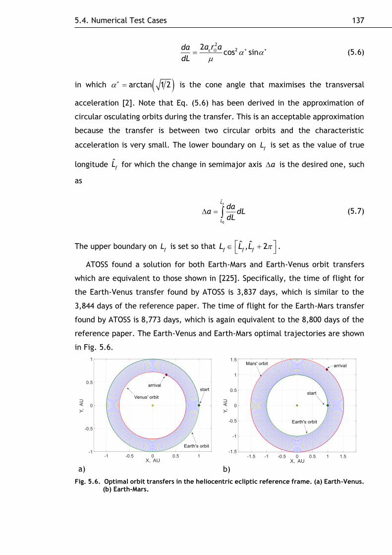
5.4. Numerical Test Cases 137
2
22c sinosc
a r ada
dL (5.6)
in which arctan 1 2 is the cone angle that maximises the transversal
acceleration [2]. Note that Eq. (5.6) has been derived in the approximation of
circular osculating orbits during the transfer. This is an acceptable approximation
because the transfer is between two circular orbits and the characteristic
acceleration is very small. The lower boundary on f
L is set as the value of true
longitude ˆf
L for which the change in semimajor axis a is the desired one, such
as
0
ˆfL
L
daa dL
dL (5.7)
The upper boundary on f
L is set so that
ˆ ˆ, 2f f f
L LL .
ATOSS found a solution for both Earth-Mars and Earth-Venus orbit transfers
which are equivalent to those shown in [225]. Specifically, the time of flight for
the Earth-Venus transfer found by ATOSS is 3,837 days, which is similar to the
3,844 days of the reference paper. The time of flight for the Earth-Mars transfer
found by ATOSS is 8,773 days, which is again equivalent to the 8,800 days of the
reference paper. The Earth-Venus and Earth-Mars optimal trajectories are shown
in Fig. 5.6.
a)
b)
Fig. 5.6. Optimal orbit transfers in the heliocentric ecliptic reference frame. (a) Earth-Venus. (b) Earth-Mars.

5.4. Numerical Test Cases 138
5.4.2. Three-NEA Rendezvous Mission: A Comparison with the
Literature
Dachwald et al. [16] presented a 3-NEA rendezvous mission, considering a sail
with a characteristic acceleration 20.3 mm sc
a . The total mission duration,
from launch until arrival to the final target body, is 9.16 years (which is 3,345
days). In that work, the sail is injected directly into an interplanetary trajectory
at Earth, with zero hyperbolic excess energy. Table 5.1 shows the properties of
all the encountered bodies. Here and in the following test cases, the estimated
sizes of the objects are calculated from the Minor Planet Center table of
conversion from absolute magnitude to diameter, considering an albedo in the
range 0.05 to 0.251.
Table 5.1. Properties of all the encounters of the sequence presented in [16]2.
Object 2004 GU9 2001 QJ142 2006 QQ56
Orbital type Apollo Apollo Aten
Semimajor axis, AU 1.001 1.062 0.985
Eccentricity 0.136 0.086 0.046
Inclination, deg 13.650 3.103 2.796
Absolute magnitude 21.2 23.7 25.9
Estimated size, m 170-380 50-120 10-40
EMOID, AU 0.0006 0.0094 0.0152
PHA Yes No No
NHATS No Yes No
ATOSS has been used to find a solar-sail trajectory for the same list of
encounter bodies to validate the proposed optimiser. ATOSS has been used
considering both a timed and a non-timed sequence as an input. In the first case,
the mission parameters of the reference work were used to produce the timed
sequence needed by ATOSS. This has been done to check whether ATOSS can
1 Data available online at http://www.minorplanetcenter.net/iau/lists/Sizes.html [retrieved 08
August 2015].
2 Data available online at https://cneos.jpl.nasa.gov/orbits/elements.html [retrieved 08 August 2015].

5.4. Numerical Test Cases 139
reproduce and refine the trajectory of the reference work by starting from the
same timed sequence. In the second case, instead, only the list of objects and the
departing date from the reference work have been given as an input to ATOSS.
This has been done to check whether ATOSS can find a similar solution to that
shown in [16] without any external input. Since the objects in the non-timed
sequence are NEAs, it has been chosen to consider only the time of flight given by
the law to maximise the rate of change of the inclination to generate the
preliminary timeline within ATOSS. In fact, Table 5.1 shows that the differences
in semimajor axis and eccentricity are small for the objects under consideration,
whereas there are significant differences in inclination. For both cases, the
shaped-trajectory variant of the shape-based approach was used to generate the
initial-guess solution and SNOPT was used as NLP solver.
The features of the mission are described in Table 5.2 for the case of the timed
sequence used as an input for ATOSS. Figure 5.7a shows the trajectory of the first
leg from Ref. [16], whereas the corresponding trajectory found by ATOSS is shown
in Fig. 5.7b. ATOSS found a solution for which the total mission duration is 8.46
years (i.e. 3,090 days), which is almost a year less than that proposed in [16].
However, the time spent at the first object, which is also classified as a PHA, is
the minimum allowed by the optimiser (i.e. two days). Even though this value of
the stay time is in line with the mission requirements (see Section 4.5), more time
might be needed at the object. If this is the case, a slower mission was found in
the same optimisation run which is one of the intermediate results of the
optimisation strategy shown in Fig. 5.4. The characteristics of this mission are
shown in Table 5.3. In this case, the total mission duration is 8.82 years (i.e. 3,220
days), spending 50 days at 2004 GU9. Such a mission is still approximately 120 days
shorter than the reference one. Note that ATOSS gives the possibility to set the
minimum allowed stay time at each object. Therefore, if a longer stay time at the
object is needed, this can be set and a new optimisation run.

5.4. Numerical Test Cases 140
Table 5.2. Mission parameters for the optimal 3-NEA rendezvous (values in brackets are those presented in [16] and used as timed sequence for ATOSS).
Object Stay time, days Start End Time of flight, days
Earth --- 16 May 2020
(28 Nov 2019)
13 May 2023
(13 Dec 2022)
1093
(1111)
2004 GU9 2
(113) 15 May 2023
(05 Apr 2023)
28 Jan 2027
(30 Jan 2027)
1354
(1396)
2001 QJ142 133
(90) 10 Jun 2027
(30 Apr 2027)
31 Oct 2028
(24 Jan 2029)
509
(635) 2006 QQ56 ---
Table 5.3. Mission parameters for the optimal 3-NEA rendezvous, longer mission (values in brackets are those presented in [16] and used as timed sequence for ATOSS).
Object Stay time, days Start End Time of flight, days
Earth --- 27 Mar 2020
(28 Nov 2019)
12 Feb 2023
(13 Dec 2022)
1053
(1111)
2004 GU9 50
(113) 03 Apr 2023
(05 Apr 2023)
30 Jan 2027
(30 Jan 2027)
1398
(1396)
2001 QJ142 106
(90) 16 May 2027
(30 Apr 2027)
19 Jan 2029
(24 Jan 2029)
614
(635) 2006 QQ56 ---
a)
b)
Fig. 5.7. Trajectory of the first leg from Earth to 2004 GU9. Heliocentric ecliptic reference frame. (a) Ref. [16] (Reproduced with permission of Springer). (b) ATOSS with timed sequence as an input.

5.4. Numerical Test Cases 141
In the second case, in which a non-timed sequence was used as an input, ATOSS
found a solution by self-generating the preliminary timeline for the encounters.
The total mission duration found by ATOSS is 8.83 years (i.e. 3,223 days), which is
about 120 days less than that shown in [16]. Table 5.4 shows the characteristics
of this mission together with the preliminary timeline self-generated by ATOSS.
Note that the sailcraft spends more than 90 days at each object, which is a stay
time equivalent to that shown in the reference paper.
Table 5.4. Mission parameters for the optimal 3-NEA rendezvous in the case of a non-timed sequence as an input (values in brackets are those self-generated by ATOSS).
Object Stay time, days Start End Time of flight, days
Earth --- 04 Mar 2020
(28 Nov 2019)
24 Dec 2022
(19 Dec 2022)
1026
(1117)
2004 GU9 99
(100) 02 Apr 2023
(29 Mar 2023)
23 Oct 2026
(12 Sep 2026)
1300
(1263)
2001 QJ142 111
(100) 11 Feb 2027
(21 Dec 2026)
30 Dec 2028
(04 May 2028)
688
(500) 2006 QQ56 ---
5.4.3. Multiple NEA Rendezvous Missions
The test cases studied in this subsection aim to show some fully-optimised
trajectories for a multiple NEA rendezvous mission. Because of the Gossamer
requirements discussed in Section 4.5, a solar sail with a characteristic
acceleration 20.2mm sc
a is considered throughout this subsection. Therefore,
from the results of the sequence search shown in Section 4.6 with 20.2mm sc
a
, two sequences have been selected as samples and fully optimised. The first
sequence has been selected among all the sequences found with five encounters,
of which one is a PHA and the last object is small, as from the mission
requirements a) – c) in Section 4.5. This sequence is one of those found for the
PHA-NHATS database. On the other hand, the second sequence has been chosen
among the results of the PHA-LCDB database. This sequence has been chosen
because it is characterised by the presence of two PHAs and all the target orbits
are significantly more eccentric than the one of the Earth, despite it has only
three encounters.

5.4. Numerical Test Cases 142
Sequence 1. The first sequence presented here contains five objects. All the
objects in the selected sequence are part of the NHATS database used and the
fourth, 2008 EV5, is also classified as a PHA. Table 5.5 shows the encountered
bodies in the sequence. Note that, in Table 5.5, the change in inclination between
two consecutive objects is always less than 5 deg, which is the threshold used for
the coplanar approximation [Eq. (4.16)]. However, Table 5.5 shows that the
inclination of the encounter’s orbits increases by moving from an object to the
following, eventually reaching an inclination of about 10 deg for the last
encounter. This result is significantly different respect to what could be found by
following the sequence search method described in [197], in which a threshold of
5 deg on the maximum inclination was considered within the pruning of the whole
database. Therefore, this sequence could not have been found because the last
three asteroids have an inclination larger than the 5 deg threshold.
Table 5.5. Properties of the encounters of sequence 11.
Object 2000 SG344 2015 JD3 2012 KB4 2008 EV5 2014 MP
Orbital type Aten Amor Amor Aten Amor
Semimajor axis, AU 0.977 1.058 1.093 0.958 1.050
Eccentricity 0.067 0.009 0.061 0.083 0.029
Inclination, deg 0.111 2.730 6.328 7.437 9.563
Absolute magnitude 24.7 25.6 25.3 20 26
Estimated size, m 35-75 20-50 20-50 260-590 17-37
EMOID, AU 0.0008 0.054 0.073 0.014 0.020
PHA No No No Yes No
NHATS Yes Yes Yes Yes Yes
By following the optimisation steps described in Section 5.3, a multi-phase
solution was found. ATOSS has been used with the NLP solver WORHP and the
shaped-trajectory variant of the shape-based approach as the initial-guess
solution. The parameters of the optimised mission are briefly described in Table
5.6. The values in brackets are the results of the sequence search algorithm, which
have been used as the timed sequence needed by ATOSS. Note that the stay time
1 Data available online at https://cneos.jpl.nasa.gov/orbits/elements.html [retrieved 08 August
2015].

5.4. Numerical Test Cases 143
in brackets is always equal to 100 days, since it is a fixed value, as specified in
Section 4.6.1. The sail is injected directly into an interplanetary trajectory at
Earth, with zero hyperbolic excess energy. The mission is completed in about 8.6
years after departing from Earth on 05 December 2025. As shown in Table 5.6, the
sail spends at least three months in the proximity of each object, giving sufficient
time for close-up NEA observations.
It is worth noting that the arrival at 2014 MP after 3,133 days is not necessarily
the end of the mission. As long as the sailcraft remains flightworthy, the visit at
2015 MP may well be followed by further legs to other NEAs. In fact, the duration
of the mission is not constrained by the amount of propellant on board, as it
usually happens when an electrical or chemical propulsion system is used. It only
depends on the ageing of the systems aboard and the will to pay the flight
operators a while longer for their effort. For instance, Pioneer 6 was designed to
last about 6 months, after its launch on 16 December 1965. The last successful
contact with it was made on 08 December 2000 – 35 years later. In 1997, three of
its instruments still worked well1.
Table 5.6. Mission parameters for optimised sequence 1 (values in brackets are those found through the sequence search algorithm and used as a first guess for ATOSS).
Object Stay time, days Start End Time of flight, days
Earth --- 05 Dec 2025
(30 Apr 2025)
18 Mar 2027
(11 Mar 2027)
468
(680)
2000 SG344 93
(100) 19 Jun 2027
(19 Jun 2027)
03 Nov 2028
(31 Oct 2028)
503
(500)
2015 JD3 104
(100) 16 Feb 2029
(08 Feb 2029)
22 Nov 2030
(14 Nov 2030)
644
(644)
2012 KB4 94
(100) 23 Feb 2031
(22 Feb 2031)
22 Nov 2032
(30 Nov 2032)
637
(647)
2008 EV5 95
(100) 25 Feb 2033
(10 Mar 2033)
04 Jul 2034
(25 Nov 2034)
493
(625) 2014 MP ---
1 Data available online at https://www.nasa.gov/centers/ames/missions/archive/pioneer.html
[retrieved 15 June 2017].

5.4. Numerical Test Cases 144
The complete trajectory of the optimised sequence 1 is shown in Fig. 5.8. The
stay times at the objects are highlighted against the interplanetary legs. The orbit
of the Earth is also plotted. Plots of the control histories on each leg are in Fig.
5.9. The three components of the acceleration vector in the orbital reference
frame over time are shown, together with the magnitude of the acceleration over
time.
a)
b)
Fig. 5.8. Heliocentric view of the 3D trajectory of optimised sequence 1: (a) ecliptic plane view; (b) 3D view.

5.4. Numerical Test Cases 145
a) b)
c) d)
e)
Fig. 5.9. Acceleration components history on each transfer leg of optimised sequence 1.
It is worth noting that, despite the few spikes in the control history shown in
the plots in Fig. 5.9, the results are feasible by a solar sail with currently-available
technology. This can be demonstrated by studying both slew rate and angular
acceleration of the sail required to follow the control histories shown in Fig. 5.9.
Denoting the angle as the angle between two consecutive attitudes [i.e.
1
ˆ ˆarccosi i
t tN N ], the sail slew rate is defined as the rate of change
of the sail attitude. Figure 5.10a shows the sail slew rate for the last leg of the
current five-NEA sequence. This leg has been chosen because it is the one with
the highest value of slew rate. Figure 5.10a shows that the sail slew rate is always
43 10 deg s. Studies on solar-sail attitude control in the literature show
that a solar sail with a characteristic acceleration of 20.1 mm sc
a is able to
perform a 35 deg manoeuvre in less than 3 hours [48, 226], thus with an average
sail slew rate of 35 10 deg s . Moreover, Wie and Murphy [226] show that

5.4. Numerical Test Cases 146
the spike in the slew rate for a 35 deg yaw manoeuvre is max
0.03 deg s , which
is higher than the maximum slew rate required during the whole mission described
here.
The angular acceleration needed to follow the control found through ATOSS
shall also be investigated to verify the feasibility of such a mission from the
attitude-control point of view. Figure 5.10b shows the angular acceleration for
the last transfer leg of the first optimised sequence, obtained by time
differentiation of the sail slew rate shown in Fig. 5.10a. It is possible to see a spike
in the angular acceleration, related to the first pick in the slew rate, of
9 2 d2 0 eg s1 . For comparison, note that the maximum torque allowed for
a Mars rendezvous mission in [227] (pp. 69-86) is set to 3
max10 Nm . Because a
solar sail with an area 2
160 mA and a total mass 0
450 kgm is considered in
the aforementioned work, the equivalent maximum allowed angular acceleration
is 8 2
max6 1 deg s0 , considering a perfect square sail rotating around one of
the principal axes of inertia on the sail plane. Such value is larger than the
maximum sail angular acceleration needed to achieve the proposed transfers (Fig.
5.10b).
Because no explicit constraints have been set on either the sail slew rate or
the angular acceleration within ATOSS, further optimisation may be needed if
stricter constraints are required.
a) b)
Fig. 5.10. Sail slew rate (a) and sail angular acceleration (b) over time on the last leg of optimised sequence 1.

5.4. Numerical Test Cases 147
From a trajectory optimisation point of view, it is interesting to study the
evolution of the total mission duration during the second stage of the optimisation
strategy implemented within ATOSS. As detailed in Section 5.3.2, once the entire
multi-phase 3D trajectory has been found, a discrete continuation on the lower
boundary on the final time is carried out to find a solution with a lower total
mission duration. Figure 5.11 shows the evolution of the total mission duration
within ATOSS. The total cumulative computational time needed to find a solution
is shown along the horizontal axis. Each point in the figure corresponds to a
solution found by ATOSS in each intermediate step. The first point is related to
the mission duration of the entire trajectory obtained by patching together the
initial-guess trajectories for each transfer leg. Note that the significantly longer
time related to the second point is due to ATOSS finding a 3D multi-phase
trajectory starting from the solutions of the shape-based approach, which is the
first stage of the optimisation strategy described in Section 5.3.2 and shown in
Fig. 5.5. In conclusion, Fig. 5.11 demonstrates the importance of the continuation
stage implemented within ATOSS, which decreases the total mission duration by
10% respect to the value of the initial guess. In fact, a gain of 6% of total mission
duration is achieved during the second stage of the optimisation strategy
developed within ATOSS (i.e. between the last and the second point shown in Fig.
5.11).
Lastly, the end-to-end optimisation phase, as described in Section 5.3, needed
about four hours of computational time. It is important to note, however, that
this is the overall time required by ATOSS and it includes the time spent within
the optimiser when the convergence was not achieved, other than the generation
of the initial guesses. If the time spent by the optimiser to find the shown
trajectory is considered alone, a total time of about half an hour is needed for the
end-to-end optimisation of the entire multi-leg trajectory, as shown in Fig. 5.11.

5.4. Numerical Test Cases 148
Fig. 5.11. Evolution of the total mission duration within ATOSS for optimised sequence 1.
Sequence 2. The second sequence contains three objects. This sequence has
been chosen among the others because it is characterised by the presence of two
PHAs, 1989 UQ and 2002 RW25. The first object of the sequence, 2003 WT153, is
part of the LCDB database with 2U . All the objects are Aten asteroids. That
is, their semimajor axes are all less than one astronomical unit. Moreover, the
orbits of all the encounters in the sequence are significantly more eccentric than
the one of the Earth, as shown in Table 5.7.

5.4. Numerical Test Cases 149
Table 5.7. Properties of the encounters of sequence 21.
Object 2003 WT153 1989 UQ 2002 RW25
Orbital type Aten Aten Aten
Semimajor axis, AU 0.894 0.915 0.825
Eccentricity 0.178 0.265 0.287
Inclination, deg 0.371 1.299 1.327
Absolute magnitude 28 19.4 18.8
Estimated size, m 7-15 330-740 420-940
EMOID, AU 0.002 0.014 0.016
PHA No Yes Yes
A multi-phase trajectory for the selected solar sail has been found by following
the optimisation steps described in Section 5.2 and the mission is summarised in
Table 5.8. The sailcraft needs 3,541 days (i.e. 9.7 years) to reach all asteroids in
this sequence, after spending more than three months in the proximity of each.
Figure 5.12 shows the two-dimensional projection of the complete 3D
trajectory of the chosen sequence. Plots of single-leg trajectories and controls
over time are not shown for the sake of brevity.
Table 5.8. Mission parameters for optimised sequence 2 (values in brackets are the ones found through the sequence search algorithm and used as an initial guess for STO).
Object Stay time, days Start End Time of flight, days
Earth --- 24 Apr 2028
(14 Apr 2028)
18 Jul 2031
(01 Oct 2031)
1181
(1265)
2003 WT153 134
(50) 30 Nov 2031
(20 Nov 2031)
29 Jun 2034
(19 Aug 2034)
943
(1003)
1989 UQ 110
(50) 18 Oct 2034
(08 Oct 2034)
02 Jan 2038
(19 Mar 2038)
1173
(1258) 2002 RW25 ---
1 Data available online at https://cneos.jpl.nasa.gov/orbits/elements.html [retrieved 08 August
2015].

5.4. Numerical Test Cases 150
Fig. 5.12. Heliocentric view of the complete three-dimensional trajectory of optimised sequence 2 (ecliptic plane view).
The total v needed for this mission is 52.1 km sv , which has been
calculated as the integral of the acceleration over time. Despite such a high v
is the result of a control law optimised for solar sailing, it is interesting to compare
with an electric propulsion system. As such, consider the spacecraft used in the
8th Global Trajectory Optimisation Competition (GTOC8) [175, 228]. This
spacecraft is characterised by a total mass 0
4,000 kgm , a dry mass
1,890 kgdry
m and a low-thrust engine with a specific impulse 5,000 sspI . It is
worth noting that both the specific impulse and the mass ratio 0
0.47dry
m m
considered are very high performing and no spacecraft, to the best of the author’s
knowledge, has similar performances to date. Recall the Tsiolkovsky rocket
equation as [229]
00ln
sp
f
mg
mv I (5.8)
in which, in this case, the final mass f
m is considered as the spacecraft dry mass
drym . By using Eq. (5.8), the maximum v available with such low-thrust system

5.4. Numerical Test Cases 151
is 37 km sv . On the other hand, to reach a v as high as 52 km s , a
spacecraft with the electric propulsion system considered in the GTOC8 should be
characterised by a mass ratio as low as 0
0.35dry
m m , which is very low for the
near-term electric-propulsion technology. For the above reasons, a multiple NEA
rendezvous mission with a total 52 km sv is not feasible by an electric
propelled spacecraft, even if a high-performing propulsion system is considered.
A solar sail, on the other hand, enables high-v trajectories such as the one
shown.
5.4.4. Multiple NEA Sample Return Mission
The optimised sequence 1 described in Section 5.4.3 has been considered to
study the potential for a multiple NEA sample return mission. To do so, the last
leg to 2014 MP has been removed and substituted with a return leg to the Earth.
STO was used to compute the return leg to the Earth. The total mission duration
is now 3,821 days (which is about 10.5 years), which is still compatible with the
ten-year mission requirements described in Section 4.5. The return leg to the
Earth is shown in Fig. 5.13, whereas Table 5.9 shows the updated mission
parameters.
It is worth noting that the sequence still contains 2008 EV5, which is classified
as a PHA and was selected as one of the candidate targets for the Asteroid Redirect
Robotic Mission (ARRM) by NASA [230]. Moreover, the stay time at 2008 EV5 is
above 100 days, which is the longest of this sequence of asteroids.
Fig. 5.13. Heliocentric view of the 3D return leg to the Earth.

5.4. Numerical Test Cases 152
Table 5.9. Mission parameters for the optimised sequence 1 with the last leg to the Earth.
Object Stay time, days Start End Time of flight, days
Earth --- 05 Dec 2025 18 Mar 2027 468
2000 SG344 93
19 Jun 2027 03 Nov 2028 503
2015 JD3 104
16 Feb 2029 22 Nov 2030 644
2012 KB4 94
23 Feb 2031 22 Nov 2032 637
2008 EV5 116
18 Mar 2033 22 May 2036 1161
Earth ∞
5.4.5. Online Change of the Mission: Two Test Cases for the
Planetary Defence
Two test cases have been studied as possible mission scenarios in response to
the mission exercises proposed by the planetary defence community. In both test
cases, the sailcraft is considered already flying to its planned mission to several
NEAs, when a PHA appears to gain interest over the worldwide community.
Therefore, the mission control decides to reroute the sailcraft to rendezvous or
flyby with such object. This will also demonstrate the target flexibility unique to
solar sailing. In the following subsections, the two test cases are discussed in
detail.
Test Case 1: 2011 AG5. During the 3rd International Academy of Astronautics
(IAA) Planetary Defense Conference (PDC) held in Flagstaff, AZ, USA in 2013, the
asteroid 2011 AG5 was considered as one of the reference scenarios to conduct an
exercise to respond to a hypothetical asteroid threat1. At the time of the
conference, the asteroid had a probability of impact with the Earth of 1 in 500
(i.e. 32 10 ) on 05 February 2040 [231], and the value of the object on the
Palermo scale [232] was 1P , which indicates that the PHA merits careful
1 Data available online at http://pdc.iaaweb.org/?q=content/2013-flagstaff [retrieved 15 June
2017].

5.4. Numerical Test Cases 153
monitoring. In fact, only two objects among all the ones studied in [232] had a
value 1P .
The first multiple NEA rendezvous mission discussed in Section 5.4.3 has been
considered as the baseline for the current scenario. That is, in the hypothesis that
the mission is flying as scheduled, the last leg to 2014 MP shown in Table 5.6 is
replaced to a leg to the potentially-hazardous asteroid 2011 AG5. Note that,
according to Chodas et al. [231], a deflection that will take place after 03
February 2023 is about 50 times harder than before such date. Nevertheless, the
rerouted sailcraft will inevitably reach the PHA after that date, since the entire
baseline mission starts on 2025 (Table 5.6). The solar sail can easily change its
route and reach 2011 AG5 before the potential predicted impact with the Earth,
thus providing detailed updates on the asteroid and its course. Moreover, this will
be performed at the only cost of the last asteroid not being visited as scheduled.
However, if 2011 AG5 will not collide with the Earth and destroy the mission
control centre, the sailcraft could be, in principle, still rerouted to its original
mission. Table 5.10 shows the properties of 2011 AG5.
Table 5.10. Properties of 2011 AG51.
Object 2011 AG5
Orbital type Apollo
Semimajor axis, AU 1.431
Eccentricity 0.390
Inclination, deg 3.681
Absolute magnitude 21.8
Estimated size, m 110-240
EMOID, AU 0.0002
PHA Yes
NHATS No
To find the transfer leg to the new target, the homotopic approach to solar
sailing, described in Section 3.2, has been used at first. Firstly, a constant-mass
low-thrust transfer between 2008 EV5 and 2011 AG5 has been computed by means
1 Data available online at https://cneos.jpl.nasa.gov/orbits/elements.html [retrieved 08 August
2015].

5.4. Numerical Test Cases 154
of the indirect optimisation approach. The time of flight and the initial values of
the costates have been determined through the PSO algorithm described in
Appendix B.2. For this scenario, the orbits of both objects are considered
coplanar. That is, the orbital plane of 2011 AG5 has been rotated and projected
onto the one of 2008 EV5, as described in Eq. (3.21). Moreover, the maximum
acceleration given by the propulsion system has been set to 2
max1 mm sa .
Starting from the low-thrust solution, the homotopy-continuation approach has
been used to find a coplanar solar-sail transfer with 20.2 mm sc
a . Then, ATOSS
has been used to find the final three-dimensional trajectory by first changing the
orientation of the orbital plane and then changing its inclination.
The total mission duration is now 4,398 days (i.e. about 12 years) and the
sailcraft arrives at the final target object on 25 May 2037, about 3 years before
the potential impact. Figure 5.14 shows the last transfer leg between 2008 EV5
and 2011 AG5, whereas Table 5.11 shows the updated mission parameters. Note
that the value of the stay time related to 2011 AG5 is the time interval between
the rendezvous and the expected impact with the Earth.
Fig. 5.14. Heliocentric view of the 3D transfer leg between 2008 EV5 and 2011 AG5.

5.4. Numerical Test Cases 155
Table 5.11. Mission parameters for optimised sequence 1 with the last leg to 2011 AG5.
Object Stay time, days Start End Time of flight, days
Earth --- 10 May 2025 26 Feb 2027 657
2000 SG344 123
29 Jun 2027 06 Sep 2028 436
2015 JD3 164
18 Feb 2029 24 Sep 2030 584
2012 KB4 160
04 Mar 2031 29 Sep 2032 576
2008 EV5 7.5
07 Oct 2032 25 May 2037 1691
2011 AG5 987
Test Case 2: 2017 PDC. A second test case is considered in this subsection
which targets the fictitious PHA 2017 PDC. This has been introduced at the 5th IAA
Planetary Defense Conference held in Tokyo, Japan on 20171. The full description
of the 2017 PDC hypothetical asteroid impact scenario can be retrieved at the
JPL/NASA Center for Near Earth Object Studies (CNEOS) website2. According to
this scenario, the asteroid 2017 PDC is discovered on 06 March 2017 and, on the
following day, a potential impact of this fictitious object with the Earth is
expected to be on 21 July 2027. Two months after its discovery, the asteroid has
a probability of impact with the Earth of 1 in 100 and, therefore, its value on the
Palermo scale is 0.22P 3, which corresponds to “a situation more threatening
than the background hazard” [232]. Table 5.12 shows the properties of the
fictitious asteroid 2017 PDC.
1 Data available online at http://pdc.iaaweb.org/?q=content/2017-tokyo [retrieved 16 June
2017].
2 Data available online at https://cneos.jpl.nasa.gov/pd/cs/pdc17/ [retrieved 16 June 2017].
3 Value obtained according to [232], considering the properties of a standard NEA.

5.4. Numerical Test Cases 156
Table 5.12. Properties of 2017 PDC1.
Object 2017 PDC
Orbital type Apollo
Semimajor axis, AU 2.24
Eccentricity 0.607
Inclination, deg 6.297
Absolute magnitude 21.9
Estimated size, m 110-240
EMOID, AU 0.0008
PHA Yes
NHATS No
Note that, because of the expected date of impact, the first multiple NEA
rendezvous mission discussed in Section 5.4.3 is not a good candidate as a baseline
mission. Therefore, from the results of the same sequence search performed on
the PHA-NHATS database and discussed in Section 4.6.1, a different sequence has
been optimised and considered as a baseline mission for a leg to 2017 PDC. Table
5.13 shows the mission parameters for this optimised sequence.
Table 5.13. Mission parameters for the baseline mission for the 2017 PDC test case.
Object Stay time, days Start End Time of flight, days
Earth --- 13 Aug 2020 26 Apr 2022 621
2005 TG50 128
02 Sep 2022 13 Jan 2024 498
2015 JF11 104
25 Apr 2024 10 Jun 2026 776
2012 BB14 139
28 Oct 2026 02 Aug 2028 644
2014 YN ---
1 Data available online at
https://ssd.jpl.nasa.gov/horizons.cgi?find_body=1&body_group=all&sstr=2017+PDC [retrieved 06 March 2017].

5.4. Numerical Test Cases 157
As for the previous test case, in the hypothesis that the mission is flying as
scheduled, the sailcraft is rerouted, after the second transfer leg, to go towards
2017 PDC. The same methodology applied to the previous test case has been used,
starting from a low-thrust solution with 2
max2 mm sa . Nevertheless, the orbit
of 2017 PDC is significantly different from the one of the departing object because
of the high eccentricity and the large semimajor axis. Moreover, the time
constraint on the mission1 and the low characteristic acceleration of the sailcraft
make this scenario very difficult to solve and no feasible transfer trajectories have
been found to rendezvous 2017 PDC. In fact, a solar-sail transfer leg with
20.73 mm sc
a has been found which needs more than 2,000 days to be
performed, considering the orbit of 2017 PDC coplanar with the one of 2011 JF11.
That is, a sailcraft with a considerably larger characteristic acceleration than the
one considered in this study would arrive at the target object on 21 August 2030,
which is about three years after the predicted impact with the Earth. Figure 5.15
shows the transfer leg together with the non-dimensional acceleration vector.
Fig. 5.15. Heliocentric view of the coplanar transfer between 2015 JF11 and 2017 PDC (ac = 0.73 mm/s2).
1 After the second leg of the baseline mission, there are only three years left to reach 2017 PDC
before the impact with the Earth, if any.

5.4. Numerical Test Cases 158
Even though the sailcraft rerouting has been proven inefficient for a
rendezvous with 2017 PDC, the same (already flying) sailcraft can still be used to
target 2017 PDC for a fast flyby. Such a mission gives an extra (free) opportunity
to monitor the asteroid’s path before the expected impact, even after a potential
deflection mission takes place. In fact, if a deflection mission was successful, the
orbit of 2017 PDC would only be slightly different from the unperturbed one1.
Therefore, the unperturbed orbit of the asteroid can be safely considered for the
trajectory design.
The initial-guess solution for ATOSS has been computed by means of the
homotopy-continuation approach, starting from a low-thrust transfer with
2
max0.2 mm sa . In this case, the final spacecraft velocity is left free, since a
flyby is considered. The optimised 3D trajectory found by ATOSS is shown in Fig.
5.16, whereas Table 5.14 shows the mission parameters of the updated sequence
with the addition of the flyby to 2017 PDC. After a three-year journey, the sailcraft
reaches 2017 PDC on 07 April 2027, which is about three months before the
expected impact. Note that no stay time at 2017 PDC is considered, since the
sailcraft reaches the asteroid for a fast flyby.
Table 5.14. Mission parameters for the baseline mission for the 2017 PDC test case with the last leg to 2017 PDC.
Object Stay time, days Start End Time of flight, days
Earth --- 13 Aug 2020 26 Apr 2022 621
2005 TG50 128
02 Sep 2022 13 Jan 2024 498
2015 JF11 91
13 Apr 2024 07 Apr 2027 1089
2017 PDC ---
1 At the end of the PDC 2017 exercise, it was shown that the orbit of 2017 PDC after the
successful deflection mission was such that the asteroid would miss the Earth by about 1,000 km.

5.4. Numerical Test Cases 159
Fig. 5.16. Heliocentric view of the 3D transfer trajectory to flyby 2017 PDC.
5.4.6. Automated Optimisation Campaign
The last set of test cases aims to assess the performances of both STO and
ATOSS as automated optimisers. To do so, all the 589 preliminary sequences with
at least three encounters and at least one PHA found for the PHA-LCDB database
shown in Section 4.6.2 are optimised by means of the two optimisers developed.
Moreover, the performances of ATOSS are compared to those of the sequential
trajectory optimiser. The number of optimal solutions found and the
computational time needed for the entire automated optimisation campaign are
the two parameters used for the performance test. For the entire optimisation
campaign, the NLP solver SNOPT, together with the propagated-trajectory variant
of the shape-based approach, is used within ATOSS.
Once the initial settings are defined at the beginning of the optimisation
campaign, all the simulations are carried out with the same settings and with no
user intervention. Of course, it is likely that some of the results found can be
improved by choosing ad hoc settings for each test case so that the optimisers are
tuned for that specific scenario (see, for instance, the “no free lunch theorems
for optimisation” [233]). Nevertheless, this is beyond the scope of this work, which
aims to test the capability of the developed optimisers to find as many optimal
solutions as possible automatically. Once solutions for all the test cases have been
found, the user can choose the most interesting ones to be further optimised.

5.4. Numerical Test Cases 160
The results of the automated optimisation campaign are schematically shown
in Table 5.15. STO found a solution for 343 sequences, which is 58% of the total
number of sequences tested. On the other hand, ATOSS found fully-optimised
solar-sail trajectories for 390 sequences, which is 66% of the total number of
sequences tested. The sequences optimised through ATOSS are characterised by
84 unique NEAs. Among them, there are 58 PHAs, 11 asteroids which are part of
the NHATS database and 28 NEAs which are part of the LCDB with 2U .
STO took less than a month looking for solutions to all the 589 sequences found,
performing more than 20 optimisations per day on average. On the other hand,
when ATOSS was used on the same machine, the entire automated optimisation
campaign took less than six days of computational time.
These results demonstrate the reliability of both STO and ATOSS as automated
optimisers. Moreover, such results also demonstrate the reliability of the sequence
search algorithm described in CHAPTER 4, since more than 50% of the preliminary
sequences found are shown to be feasible. It is interesting to compare the quality
of the solutions found by the two optimisers. An estimate of the quality of the
solutions can be obtained by analysing the total mission durations found by the
two optimisers. This is done only on those sequences (292) for which both
optimisers found a solution. Two solutions are considered equivalent if the
difference in their mission durations is within twenty days. An analysis of the
numerical results showed that in 285 test cases (~98%) the solutions found by
ATOSS are shorter than those found by STO. On the other hand, STO found a
shorter solution than ATOSS in only one test case; the two optimisers found
equivalent solutions in the remaining six test cases (~2%). From the comparison of
the results found by means of the two optimisers developed, it can be seen that
ATOSS outperforms the sequential trajectory optimiser in success rate,
computational speed and quality of the solutions found. The better performances
of ATOSS in terms of success rate and computational speed are likely due to the
first stage of the optimisation strategy, which has been developed in purpose to
help the numerical convergence of the NLP solver. The second stage of the
optimisation strategy developed within ATOSS is the reason for the better
solutions, in terms of quality, found by ATOSS in comparison with those found by
STO.

5.5. Discussion 161
Table 5.15. Automated optimisation campaign results.
Optimiser Number of
solutions found Success rate Computational time
STO 343 58% < 30 days
ATOSS 390 66% < 6 days
5.5. Discussion
In this chapter, two optimisation tools have been presented which are
developed to find solutions to the solar-sailing multiple NEA rendezvous OCP. Both
optimisers have been developed with the main goal of being mostly automatic,
thus requiring minimal input from the user. This is because, at this stage of the
mission design, it is more important to have many candidate mission scenarios
rather than finding very accurate solutions.
A number of test cases demonstrated the capabilities of the two optimisers
presented. A five-NEA rendezvous mission is shown to be feasible in less than ten
years with a near-term solar sail, allowing at least three months in the vicinity of
each encounter for close-up observations. A second test case showed a mission to
rendezvous three objects on eccentric orbits. It was shown that such very mission
would not be feasible with a near-term electric propulsion system because of the
limited amount of propellant available. Furthermore, three more test cases
showed the versatility of the solar-sail propulsion system, which allows changing
the mission even after has started. The capability to change targets en-route
allows a mission already in flight to respond to either extreme events such as a
potential Earth impactor being discovered or changes in the commercial/scientific
interest. Lastly, an automated optimisation campaign demonstrated the reliability
of both optimisers to perform without any input from the user. This is a key
feature of the developed optimisers, since very often the numerical optimisation
is sensitive to the optimisation parameters. Nevertheless, ATOSS showed better
performances, in terms of success rate, computational time needed and quality
of the solutions found, than its counterpart does. This is understandable, being
ATOSS an upgrade of the sequential trajectory optimiser. Lastly, ATOSS allows
setting a minimum desired stay time at each target object. This feature can be

5.5. Discussion 162
fundamental in the mission design of a multiple NEA rendezvous, for which a
minimum time for close-up observation might be needed by the onboard
instruments.
All the numerical test cases discussed in this section not only demonstrated the
capabilities of the two optimisers developed but also revealed the potential of
solar sailing to achieve goals unattainable by a classical electric propulsion
system.

CHAPTER 6.
CONCLUSIONS
This thesis presented several techniques and methodologies for preliminary
trajectory design of multiple near-Earth asteroid (NEA) rendezvous missions
through solar sailing. This final chapter summarises the work carried out, the tools
developed, and the main findings of this thesis. Known limitations are also
discussed and directions for a possible future research are drawn.
6.1. Summary of the Work
In this thesis, the problem of preliminary mission design for solar-sail multiple
NEA rendezvous is tackled. A NEA rendezvous with close-up observations is
important to improve our knowledge about these objects. A multiple rendezvous
is even a more attractive mission because of the large population of asteroids and
the many uncertainties that still characterise them. This, however, introduces
several difficulties in the mission design, such as the potentially-high v needed.
Furthermore, the rate of NEAs’ discovery and the dynamic change in the objects
of interest make the en-route change of the target objects an appealing
perspective. As it was shown for the case of the Hayabusa-2 extended mission,
however, this is usually complicated by the amount of propellant available on
board. For this reason, solar sailing is an attractive propulsion system since its
thrust is entirely generated by reflecting sunlight and thus no onboard propellant
is needed. As such, it is well suited for a multiple rendezvous mission.
The principal objective of this thesis was to develop a tool for the preliminary
trajectory design of multiple NEA rendezvous missions through solar sailing. In
fact, not a single tool was built but several techniques, algorithms and tools were

6.1. Summary of the Work 164
developed. These can work independently or can be easily interfaced between
themselves and thus be used as a larger standalone toolbox able to perform the
required multiple-NEA rendezvous mission design from the selection of the
sequence of asteroids to the full trajectory optimisation.
The first step towards the achievement of this objective was the development
of a mathematical model for the fast representation of a solar-sail trajectory. This
is the cornerstone of the entire work as a fast and reliable trajectory model is
needed for generating preliminary sequences of encounters as well as having an
initial approximated trajectory. The shape-based approach was considered for the
description of the trajectory because it is a semi-analytical approach and no
complex and time-consuming optimal control problem (OCP) needs to be solved.
In fact, this approach consists in designing the desired shape of the trajectory by
means of a set of chosen equations. Thus, the acceleration that the spacecraft
shall provide to follow the planned trajectory is analytically retrieved a posteriori.
Because of the intrinsic differences between the thrust that can be produced by
a classical low-thrust system and a solar sail, a new set of shaping functions was
proposed for solar sailing. This was proven to give a reliable approximation of the
solar-sail trajectory on a number of NEA-to-NEA transfers. A second method was
developed which generates solar-sail trajectories starting from classical low-
thrust ones. A homotopy-continuation technique is the core of the method, which
solves several OCPs by slightly changing the acceleration model. The advantages
and drawbacks of both methods were discussed. It appeared that the shape-based
approach is better suited for finding a large number of trajectories in an
automated way, whereas the second method is more suited for complex
trajectories (such as the fast flyby of the fictitious potentially hazardous asteroid
2017 PDC).
The second step towards the completion of this thesis’ goal was to develop an
algorithm to look for possible sequences of NEAs to be visited in a multiple
rendezvous mission. In fact, it was noted that all the solar-sailing multiple asteroid
rendezvous missions studied in the literature lack an actual search for sequences
and the NEAs to visit are mostly handpicked. Therefore, an algorithm was
developed which exploits the tree-like search space given by all the possible
sequences of objects. The reason behind this choice is that this is a preliminary
mission design study and one of the expected outcomes is to provide a set of
feasible mission scenarios for the stakeholders. A tree search provides the user

6.1. Summary of the Work 165
with a large number of possible mission scenarios that can be chosen on the basis
of the current cost function (e.g. available launch date, some objects are
currently more interesting than others, etc.). Nevertheless, a complete tree
search over the whole database of known NEAs is computationally unmanageable.
For this reason, a reduced database made of asteroids interesting for the
planetary defence and for the human spaceflight was considered. This allowed a
reduction of the search-space dimensionality by more than three orders of
magnitude. Moreover, a local pruning of those branches of the tree that are more
likely to be unfeasible by means of the chosen sailcraft was performed at the
beginning of each transfer leg. This was carried out based on astrodynamics
considerations, such as the maximum change of a selected orbital element that is
feasible by the given propulsion system in the maximum allowed time. This
enabled a significant reduction of the number of objects to be considered. Some
heuristics (such as the minimum/maximum allowed transfer time) gives the user
the possibility to shape the search for sequences to suit their requirements in
terms, for instance, of computational effort or number of sequences returned. In
fact, stricter pruning criteria involve a reduced branching of the tree of feasible
sequences of NEA encounters. Lastly, the shape-based approach for solar sailing
was used to provide the trajectory within the search for sequences without the
need of solving an OCP for each transfer leg to be tested. Despite other models
are available in the literature which are faster than the shape-based approach
(e.g. ballistic Lambert arc), the trajectories generated with the shape-based
approach are more reliable. That is, there is a high probability that the
preliminary sequences found by means of the sequence search are feasible if
optimised with a refined trajectory model.
The third and last step towards the achievement of this thesis’ goal was to
develop a strategy to optimise the chosen sequences of NEAs with a refined
trajectory model. Since a shaped solar-sail trajectory was already available from
the sequence search, it was chosen to use it as an initial-guess solution for a
direct-transcription optimisation technique. Moreover, multi-phase problems are
usually easy to be dealt with if a direct optimisation method is used. Two
optimisation strategies were developed; namely the Sequential Trajectory
Optimiser (STO) and the Automated Trajectory Optimiser for Solar Sailing (ATOSS).
These focused on the automation of the optimisation itself. In fact, both strategies
require minimal input from the user and, therefore, are well suited to solve a

6.2. Summary of the Findings 166
large number of OCPs in an automated way. This is a valuable feature for a tool
for preliminary mission analysis, since a large number of possible trajectories are
usually evaluated in the preliminary phases of the mission design. Moreover,
ATOSS allows setting a minimum desired stay time at each target asteroid. This
feature can be fundamental in the mission design of a multiple NEA rendezvous,
for which a minimum time for close-up observation might be needed by the
onboard instruments. Several numerical test cases were carried out considering
both single and multiple rendezvous with NEAs. Specifically, the three-NEA
rendezvous presented by Dachwald et al. was reproduced, thus validating the
proposed optimisation strategies. Moreover, an automated optimisation campaign
was carried out which demonstrated the ability of the developed optimisers to
work autonomously. In fact, more than 500 solar-sail multiple-NEA rendezvous
OCPs were solved without any interaction with the user. This test case also
assessed the validity of the preliminary sequences returned by the asteroid
sequence search.
In the following subsection, the major findings of this thesis are highlighted
and briefly discussed.
6.2. Summary of the Findings
Solar sailing is a very attractive propulsion system, as it was highlighted in
Section 2.1. Nonetheless, this technology is not ready yet to be used as a
conventional spacecraft propulsion system. Many researchers are currently
studying solar sailing to increase its technology readiness level (TRL). For this
reason, all the solar-sailing missions that have already flown (e.g. IKAROS and
NanoSail-D) were mainly technological demonstrators. On the other hand, one of
the aims of this thesis was to look at the TRL-related problem from a different
perspective. That is, scenarios with high mission-related TRL were sought for
solar-sailing multiple NEA rendezvous. In fact, a sailcraft with lower performances
than the one considered by Dachwald et al. in their reference mission was used
throughout this thesis. In this case, lower performances are expressed in terms of
a lower characteristic acceleration. As it was shown in Section 2.1, the
characteristic acceleration is proportional to the sail area-to-mass ratio (AMR).
Achieving a high AMR is one of the technological challenges that many of the
6.2. Summary of the Findings 167
researchers on solar sailing are currently working on. This thesis showed that a
large number of interesting mission scenarios exists for a solar sail with
performances within the capabilities of current and near-term DLR/ESA Gossamer
sailcraft technology. That is, the mission-related TRL for multiple NEA rendezvous
through solar sailing was demonstrated to be larger than it was previously thought.
The results from the sequence search algorithm showed that several sequences
of target NEAs are possible for a wide window of launch dates. For instance, more
than 200 different four-NEA mission scenarios were found for each launch date
tested within a ten-year window. It is worth reminding that all the numerical test
cases shown were computed by considering a maximum mission flight time of ten
years. Such large variety of potential mission scenarios demonstrates that there
are little to no constraints on the launch window for a multiple NEA rendezvous
mission if a solar sail is considered.
Lastly, the unique characteristic of solar sailing of being propellantless was
exploited in two mission scenarios related to the planetary defence. In both cases,
it was assumed that the sailcraft was flying its planned multiple rendezvous
mission when a potential hazardous asteroid gained importance among the
worldwide community because of its increasing threat. Therefore, it was
considered to deviate the sailcraft route from its original path towards the new
target. Obviously, such a new modified mission would not be able to substitute a
mitigation mission but it would provide the planetary-defence community with
additional useful information about the asteroid. These test cases (which currently
constitute only academic exercises) demonstrated the versatility of the solar-sail
propulsion system, which can accommodate a change in the mission even after
the launch. This would be potentially very difficult for a spacecraft that uses a
classical low-thrust propulsion system because of the limited amount of propellant
on board.

6.3. Current Limitations and Future Research 168
6.3. Current Limitations and Future Research
Despite the positive results shown in this thesis, the proposed research has also
some known limitations. These might constitute a basis for a future study. In the
following subsections, the current limitations are examined and proposed
directions for a future research are outlined.
6.3.1. Current Limitations
The research presented in this thesis was aimed to address the problem of
preliminary mission design. As such, some approximations were considered which
allowed the development of the described tools and thus provided a full picture
of the solar-sailing potential for this kind of mission. The current known limitations
of this work can be divided into two main groups and are as follows.
Dynamics. The sailcraft was considered as a mass point subject only to the
gravitational pull of the Sun and the solar radiation pressure. The asteroids were
treated as massless points on Keplerian orbits around the Sun. As such, the
sailcraft was assumed rendezvousing a NEA when its state matched with the one
of the target and the gravitational interaction between the two bodies was not
modelled. As purely two-body dynamics were considered, no planetary gravity
assists were taken into account. Moreover, the sailcraft was considered injected
directly into interplanetary orbit at Earth, whereas a whole new set of solutions
arises if the possibility of having a nonzero hyperbolic excess energy at Earth is
introduced.
Solar-sail model. The work of Dachwald et al. was used as a reference for a
near-term multiple-NEA rendezvous mission feasible by a solar sail. As such, the
same model for the acceleration generated by the sailcraft was used. A different
and more detailed acceleration model might be used in a future research to refine
the baseline tools developed here. Moreover, the attitude control of the
spacecraft was not modelled and the solar sail was considered able to perform the
required orbital manoeuvres instantaneously. Despite this is not realistic, it was
shown that the trajectories found after the optimisation phase require an attitude
control effort below the allowed values found in the literature.

6.3. Current Limitations and Future Research 169
6.3.2. Proposed Future Research
Considering the current limitations of this work discussed in Section 6.3.1,
directions for further studies can be followed. Therefore, lines for a future
research are proposed here. These would further improve the tools developed for
mission design of multiple-NEA rendezvous through solar sailing, as well as give
the possibility to widen our knowledge about near-Earth asteroids and increase
the worldwide interest on solar sailing.
Proximity operations at the asteroids. A phase can be added between two
consecutive transfer legs in which proximity operations at the encounter are
investigated. This would need a model for the gravitational field of the asteroid
as well so that both the close approach and the interaction between spacecraft
and asteroid are analysed. Some studies have already been carried out for sailcraft
hovering about large asteroids [234, 235] or deploying landers for in-situ
characterisation [31, 223]. These might be considered as a good inception for the
proposed work.
Hyperbolic excess energy at Earth and gravity assist of the main bodies.
The possibility to consider a hyperbolic excess energy at Earth within the asteroid
sequence search adds three degrees of freedom to the entire search space
(namely, the three components of the spacecraft velocity vector when leaving
Earth). Other than increasing the computational effort needed to find interesting
sequences of NEAs, this potentially widens the typology of feasible missions,
allowing trajectories to more eccentric orbits. A parametric study on solar-sail
orbit transfers with the inclusion of hyperbolic excess velocity at Earth showed an
interesting relation between the optimal direction of the hyperbolic excess
velocity vector and the Lagrange multipliers [144]. This might be used as a
reference for the proposed research direction. Furthermore, also the possibility
to use one or more gravity assists of the main bodies (e.g. Earth, Moon and Mars,
in this case) increases the amount and typology of potential solar-sail missions for
multiple NEA rendezvous. A study in this direction can start by looking at the broad
literature available on multiple gravity assist trajectory planning.

6.3. Current Limitations and Future Research 170
Trajectory refinement. A third proposed direction for future study involves a
refinement of the trajectory by considering, for instance, a different solar-sail
force model or the interaction between attitude and orbital dynamics. A study in
this direction was carried out by Borggräfe within the framework of the low-thrust
trajectory optimisation software InTrance [227]. Furthermore, N-body dynamics
can be considered for the transfer trajectories, using models such as the circular
restricted three-body problem (CR3BP). As such, the gravitational influence of
major bodies like the Earth can be examined. A potential approach to this problem
is the use of a homotopy-continuation method, such as the one described in
Section 3.2. A homotopic transformation can be defined to link the dynamics of
the sailcraft in the two-body problem to the solar-sail dynamics in the CR3BP.
Solar-sail trajectory indicator. Indicators to compute equivalent v for low-
thrust cases, such as Edelbaum’s formulation for near-circular orbits [236], are
used extensively in pruning the search space for the target selection of multiple-
target mission [220]. However, as discussed in Section 4.3, the amount of v
needed for a transfer does not provide a good indication about the feasibility of
such a trajectory by means of the sailcraft under consideration. Therefore, a solar-
sail trajectory indicator can be investigated which would be the reciprocal of the
equivalent v for low thrust. As such, this can be used in addition to the pruning
criteria already developed within the sequence search, thus further reducing the
computational effort needed to compute the shaped trajectories.

APPENDIX A.
METAHEURISTIC OPTIMISATION
METHODS: A CLOSER LOOK
This appendix presents a brief description of two of the most studied
metaheuristic optimisation methods, which are the genetic algorithm and the
particle swarm optimisation. In fact, these are the two metaheuristic optimisation
methods used to find some of the results shown within this thesis. Lastly, InTrance
is briefly presented. Although it has not been used in this work, InTrance is a
promising algorithm for low-thrust trajectory optimisation. Therefore, the author
considers worthwhile giving a brief review of it.
A.1. Genetic Algorithm
GA simulates the natural selection within the biological evolution of species,
as described by Darwin’s theory. This is based on the “survival of the fittest”
concept [101] (thus the term fitness function often used instead of cost or
objective function). GA is a population-based algorithm in which each individual
(the so-called chromosome) contains all the information about the optimisation
variables. First, an initial population is randomly generated. To find the optimum
of the desired function, an evolution process is applied on the current population
(Fig. A.1). Such evolution process consists of the following steps [101]:

A.1. Genetic Algorithm 172
Evaluation: the cost function associated with each chromosome is
evaluated.
Selection: some of the chromosomes are randomly (yet with a probability
depending on their cost function) selected for reproduction.
Crossover: the selected chromosomes (parents) cross over to form new
offspring (children).
Mutation: the new offspring mutate with a set probability.
After the reproduction (i.e. crossover and mutation) is completed for all the
parents, the new population is formed and is ready to be evaluated again for a
new iteration of the evolution process. The genetic algorithm stops when some
stopping criteria are triggered (e.g. the cost function over the entire population
is almost the same, the value of the cost function did not change over the last
iterations, the maximum number of iterations is reached, etc.).
Fig. A.1. Schematic of the GA’s evolution process.
EVALUATION SELECTION
CROSSOVERMUTATION

A.2. Particle Swarm Optimisation 173
A.2. Particle Swarm Optimisation
PSO is a population-based optimisation method in which each individual (the
so-called particle) is characterised by a position r and a velocity v in the space
whose coordinates are the optimisation variables. The whole algorithm mimics a
flock of birds looking for food. Each individual knows the place in which it found
more food (which is the so-called cognitive factor) and the place in which the
largest amount of food has been found so far by the entire flock (which is the so-
called social factor). Therefore, the next place in which the bird will look for food
depends on its current position and velocity (which is the so-called inertial factor),
as well as both the cognitive and the social factors, properly weighted. Figure A.2
shows a schematic of the state (position and velocity) evolution implemented
within PSO. If the time evolution is seen as a succession of steps max
1, ,k K , the
state history of each particle 1, ,i N is described by the position ( )k ir and
velocity ( )k iv of each particle i at each step k [102]. At each step, the current
historical best position of each particle ( )k
bestip is evaluated as
( ( )) argmin kk
besti J ip (A.1)
Likewise, the current historical best position of the entire swarm ( )k
bestg is evaluated
as
( ( )) argmink
b st
k
eJg (A.2)
The velocity vector is then updated for the next step 1k as
( )( 1) ( ) ( ) (( ) )k k k k
I
k k
best bestC Si c i c i i c ip gv v r r (A.3)
in which the terms Ic , C
c and Sc are the inertial, cognitive and social weights,
respectively. These are defined as [102]
3
1
2
0.5 0.5 0,1
1.49445 0,1
1.49445 0,1S
I
C
c r
c r
c r
(A.4)

A.2. Particle Swarm Optimisation 174
in which 10,1r , 2
0,1r , and 30,1r are three independent random numbers
between 0 and 1. Note that different values of such weights can lead to different
convergence rates of the optimiser and can even make the difference between a
successful and an unsuccessful run of the PSO. Lastly, the position vector related
to the next step 1k is updated as
( 1) ( ) ( 1)k k ki i ir r v (A.5)
Fig. A.2. Schematic of position and velocity evolution implemented within PSO. The next position of each particle is influenced by the current velocity, the location of its current personal best solution pbest, and the location of the current best solution of the swarm gbest [237].
i
i
i
( )k ir
( 1)k ir
( )k
bestg
( )k
bestip
( 1)k iv
( )k iv
j
j
j
( )k jr
( 1)k jr
( )k
bestjp
( 1)k jv
( )k jv
Current velocityVelocity towards
Velocity towards
Updated velocity
( )k
bestp
( )k
bestg

A.3. InTrance 175
A.3. InTrance
InTrance (Intelligent Trajectory optimization using neurocontroller evolution)
is implemented as the fusion between ANNs and metaheuristic optimisation
methods, the so-called evolutionary neurocontroller (NC). ANNs are based on the
way the information is processed within the animal nervous systems. This process
is “massively parallel, analog, fault tolerant and adaptive” [117] and is a good
approach to solve general learning problems. ANNs need to be trained on a training
set of known exemplary input-output pairs. However, the optimisation of low-
thrust trajectories is a so-called delayed reinforcement-learning problem,
because the result of the output is visible only at the end of the integration. For
this kind of problems, usually no training sets are available and ANNs generally
fail to find a solution. For this reason, a metaheuristic optimisation algorithm is
used to test the solutions found by ANN. In particular, a GA is implemented within
InTrance but any other metaheuristic optimisation method can be, in principle,
used. GA is employed to tune the set of parameters π (the so-called neurons)
used by the NC. The evolution of the (random) initial parameters is ruled by the
fitness function that weights the input parameters on the basis of the final
trajectory, deciding which set of neurons are more promising for the optimal
solution. A schematic of the method implemented within InTrance for solving a
trajectory optimisation OCP is shown in Fig. A.3. For a more exhaustive
explanation of the evolutionary neurocontroller method, the interested reader is
referred to [117, 227].
InTrance is designed to automatically find low-thrust trajectories, exploiting
the learning behaviour of ANNs and the evolutionary characteristics of GA.
Therefore, it is a powerful tool to find preliminary solutions to missions
challenging from a design point of view, such as the solar-sail mission designed to
maximise the kinetic impact with the asteroid 2004 WR [238]. Nevertheless, one
of the main drawbacks of InTrance is the computational effort needed to find a
solution. In fact, the double loop formed by the GA and the propagation of the
equations of motion shown in Fig. A.3 is intrinsically computationally expensive.
This is not a big issue if few trajectories need to be evaluated. On the other hand,
if a large number of trajectories are needed, the computational effort needed by
InTrance to find all the solutions becomes unmanageable.

A.3. InTrance 176
Fig. A.3. Schematic of trajectory optimisation using the evolutionary neurocontroller implemented within InTrance [117].

APPENDIX B.
IMPLEMENTATION DETAILS
B.1. MATLAB and C: A Performances Study
The asteroid sequence search described in CHAPTER 4 is mostly coded in
MATLAB. The analytical ephemerides are coded in C and interfaced with MATLAB
through MEX functions, as described in [170]. Because of the significant number
of times the ephemerides are needed within the asteroid sequence search, this
choice was straightforward for a first speedup of the entire sequence search.
However, a further action was needed in the code implementation for an
additional decrease in the computational effort needed. Therefore, a study was
carried out to locate the bottlenecks within the algorithm implementation. That
is, a test run of the asteroid sequence search, as described in Algorithm 4.1, was
carried out by setting the maximum depth of the BS to one (i.e. only the first leg
of the multiple rendezvous mission was sought). The MATLAB built-in function
profile was used to profile the execution time of all the functions called. The
entire run took about 3.5 hours, the majority of which spent to compute the
shaping functions. Specifically, the function that computes the Cartesian
acceleration [Eq. (3.23)] was called almost 500,000 times for an overall time of
more than 6,600 s. That is, more than 50% of the overall runtime was spent in
computing r . Therefore, the function related to Eq. (3.23), as well as the one
that computes the velocity vector [Eq. (3.5)], was implemented in C and a new
test run was carried out. This time, the entire run took about 96 minutes, which
is less than 50% of the previous test. The MATLAB profile highlighted the function
that computes the boundary conditions [Eq. (3.18)] as the one that took the
longest computational time. In fact, being called within a Newton loop (i.e. the

B.1. MATLAB and C: A Performances Study 178
MATLAB built-in function fsolve) inside a GA, this function was called almost
17,000,000 times for a total time of about 1,350 s (which is the 23% of the overall
runtime). A third test run was carried out with the C implementation of the
boundary-condition function. This took about 71 minutes, the 61% of which spent
inside the fsolve function. Therefore, the modified version of the Levenberg-
Marquardt algorithm implemented within the MINPACK C subroutine lmdif1 was
used instead of the MATLAB counterpart fsolve. That is, the entire function that
computes the nonlinear constraints for GA is now coded in C and interfaced with
MATLAB through a MEX function. A last test run was carried out which took 13
minutes in total. The combined MATLAB/C implementation was able to reduce by
94% the computational effort needed by the original MATLAB code. A graphical
view of the computational times for the four aforementioned test runs is shown
in Fig. B.1.
Fig. B.1. Computational times needed for the computation of the first leg of the asteroid sequence search considering four different implementations of the shape-based approach.
1 Data available online at http://www.netlib.no/netlib/minpack/lmdif.f [retrieved 23 November
2014].

B.2. PPSO: Peloni Particle Swarm Optimiser 179
B.2. PPSO: Peloni Particle Swarm Optimiser
Following the PSO algorithm presented by Pontani and Conway [102], PPSO has
been implemented in MATLAB. It is freely available online at
https://uk.mathworks.com/matlabcentral/fileexchange/58895-ppso under the
BSD 2-Clause License. PPSO has been implemented to have a custom alternative
to the MATLAB built-in functions for GA and PSO, which are ga and particleswarm,
respectively. Therefore, no extra effort has been put to optimise the
implementation and the algorithm itself. Moreover, at the time PPSO was firstly
implemented, there was no MATLAB built-in function for the particle swarm
optimisation.
A number of numerical cases have been tested to assess the reliability of the
PPSO implementation. PPSO does not explicitly handle nonlinear constraints and
thus the test cases are chosen accordingly. Moreover, both a parallelised and a
vectorised version of the algorithm are implemented within PPSO to have the
possibility to reduce the total runtime needed. For the test cases presented here,
the standard sequential non-vectorised version of the code is used. In the
following subsections, the test cases are briefly described and the results shown.
A.1.1. Test Case 1: Rastrigin’s Function
Test case 1 is the Rastrigin’s function, which is the example used in the MATLAB
User’s Guide [204] to show how to minimise a function with the GA. Two
independent variables 1x and 2
x are used for this test case. Thus, the objective
function is
1
2
2
2
1 22 1, 20 10 cos 2 cos 2J x x xx xx (B.1)
and the known global minimum is 1 2, 0,0 0J x x J . The performances of
PPSO are compared with those of the MATLAB built-in functions ga and
particleswarm. Table B.1 shows the non-default settings considered. Because of
the statistical convergence of the metaheuristic optimisation algorithms, each
optimiser is run 100 times. The number of times the optimiser finds the optimum
(which is, the success rate), within the set tolerance opt
, is the measure of the
performances used for this test case.

B.2. PPSO: Peloni Particle Swarm Optimiser 180
Table B.1. PPSO Test Case 1: Non-default settings.
Setting Value
Optimiser’s function tolerance 810
Maximum number of iterations max
K 500
Population size 25 (PPSO and particleswarm), 100 (ga)
opt
310
The results of Test case 1 are shown in Table B.2. The average number of function
evaluations among the successful runs only is used as an estimate of the
optimisers’ speed. This is done to avoid external factors that might affect the
results. However, it has been noted that the rankings based on the average
number of function evaluations mirror those based on the cpu time. For what
concerns the success rate, it can be seen that PPSO is the most reliable optimiser
among those tested. Regarding the speed, PPSO rates second in the ranking.
Table B.2. PPSO Test Case 1: Results.
Optimiser Success Rate Average Function Evaluations
PPSO 100% 7014
ga 78% 9427
particleswarm 95% 3068
A.1.2. Test Case 2: Simple Function of Two Variables
Test case 2 is the example used in the MATLAB User’s Guide [204] to show how
to minimise a function with the built-in function particleswarm. Two independent
variables 1x and 2
x are used for this test case. Thus, the objective function is
1 22
2 2
1 1, expJ x x x x x (B.2)
and the known global minimum is 1 2, 2 2,0 0.4289J x x J . The
performances of PPSO are compared with those of the MATLAB built-in functions
ga and particleswarm. Table B.3 shows the non-default settings considered. As in
the previous case, each optimiser is run 100 times.

B.2. PPSO: Peloni Particle Swarm Optimiser 181
Table B.3. PPSO Test Case 2: Non-default settings.
Setting Value
Optimiser’s function tolerance 810
Maximum number of iterations max
K 500
Population size 30 (PPSO and particleswarm), 100 (ga)
opt
310
The results of Test case 2 are shown in Table B.4. For what concerns the success
rate, it can be seen that PPSO is the most reliable optimiser among those tested.
Regarding the speed, PPSO rates second in the ranking.
Table B.4. PPSO Test Case 2: Results.
Optimiser Success Rate Average Function Evaluations
PPSO 77% 4446
ga 74% 7759
particleswarm 10% 1607
A.1.3. Test Case 3: CEC 2005
Test case 3 aims to test the performances of PPSO against some of the test
functions considered for the Congress on Evolutionary Computation (CEC) 2005
[239]. The functions 1 – 6 and 8 – 14 are tested, considering the problem dimension
10D . The interested reader is referred to [239] for a detailed description of the
single functions. Each function is tested 25 times and the success rate is used as
a performance index. Also in this case, PPSO is compared to ga and particleswarm.
Moreover, the two versions of PSO that competed in CEC 2005 are used as a further
comparison. These are: 519-PSO [240] and 620-PSO [241] (the names are those
given by the congress organisers as unique identifiers).
Table B.5 shows the results of Test case 3. Note that, on average, PPSO
performs better than the two MATLAB built-in optimisers and in line with the
results of the two PSO that took part in the competition. In fact, PPSO is able to
find more solutions than 519-PSO and 620-PSO for more than one test function.
Moreover, PPSO was coded using a standard implementation of the particle swarm
theory, whereas both 519-PSO and 620-PSO were implemented with the purpose
to improve the standard implementation of PSO.

B.2. PPSO: Peloni Particle Swarm Optimiser 182
Table B.5. PPSO Test Case 3: Results.
Function PPSO particleswarm ga 519-PSO 620-PSO
1 96% 100% 100% 100% 100%
2 100% 100% 96% 100% 100%
3 0% 0% 0% 0% 100%
4 92% 0% 0% 100% 0%
5 100% 100% 0% 100% 80%
6 4% 12% 0% 0% 100%
8 0% 0% 0% 0% 100%
9 0% 0% 8% 0% 0%
10 0% 0% 0% 0% 0%
11 0% 0% 0% 0% 76%
12 16% 8% 0% 0% 0%
13 0% 0% 0% 0% 0%
14 0% 0% 0% 0% 88%
A.1.4. Test Case 4: Optimal Two-Impulsive Transfer between
Two Circular Orbits
Test case 4 aims to test PPSO on a simple space-trajectory problem. This test
case, which is the second example in [102], describes a two-impulsive transfer
between two circular orbits. The goal is to find the impulsive thrust, in terms of
magnitude and direction, such that the total v is minimised. In this case, the
optimal known solution is given by the Hohmann transfer. Therefore, a run is
considered successful if the difference between the total v found by the
optimiser and the known optimal one is less than a set tolerance opt
. Defining
as the ratio between arrival and departing radius, ten scenarios are considered
with 2, ,11, as in the reference paper. For each scenario, both PPSO and ga
are used and run 100 times. Table B.6 shows the non-default settings used for the
two optimisers, whereas Table B.7 shows the results in terms of success rate and
average function evaluations.

B.2. PPSO: Peloni Particle Swarm Optimiser 183
Table B.6. PPSO Test Case 4: Non-default settings.
Setting Value
Optimiser’s function tolerance 1010
Maximum number of iterations max
K 500
Population size 30 (PPSO), 100 (ga)
opt
1010
Table B.7. PPSO Test Case 4: Results.
PPSO ga
Success
Rate
Average Function
Evaluations
Success
Rate
Average Function
Evaluations
2 100% 8,124 0% ---
3 100% 8,179 0% ---
4 100% 8,315 0% ---
5 100% 8,536 3% 5,332
6 100% 8,324 6% 5,329
7 100% 8,719 7% 5,326
8 100% 8,658 9% 5,325
9 100% 9,018 9% 5,327
10 100% 8,974 11% 5,335
11 100% 8,883 13% 5,324
A.1.5. Test Case 5: Bi-Impulsive Earth-Apophis Transfer
In the last test case, the bi-impulsive Earth-Apophis transfer described in [110]
is considered. Three values for the population size are considered for both PPSO
and ga, as done in the reference paper. In this case, each optimiser is run 200
times and a solution is considered optimal if the value of the objective function
differs from the known optimum by at most opt
. A maximum number of function
evaluations is allowed for each test, as shown in Table B.8. Table B.9 shows the
results, in terms of success rate, compared with the three versions of PSO
described in [110], namely PSOn05, PSOn07 and PSOn09 with 5,10,20n
depending on the population size considered. Note that, if a population of 10
particles is considered, PPSO performances are inferior to the others. For the case

B.2. PPSO: Peloni Particle Swarm Optimiser 184
of a population of 20 particles, the performances of PPSO are in line with the
other optimisers. Lastly, the success rate of PPSO with a population size of 40
particles is the best one.
Table B.8. PPSO Test Case 5: Non-default settings.
Setting Value
Maximum number of function
evaluations 10,000
Population size 10, 20, 40 (PPSO), 100, 200, 400 (ga)
opt
310
Table B.9. PPSO Test Case 5: Results.
Optimiser Population Size Success Rate
PPSO 10 25.5%
PPSO 20 36%
PPSO 40 62%
ga 100 22%
ga 200 44%
ga 400 53%
PSO505 10 35.5%
PSO1005 20 34.5%
PSO2005 40 41%
PSO507 10 39.5%
PSO1007 20 42.5%
PSO2007 40 41%
PSO509 10 43.5%
PSO1009 20 38.5%
PSO2009 40 42%

REFERENCES
[1] Jahn, R. G. and Choueiri, E. Y., “Electric Propulsion”, Encyclopedia of Physical Science and Technology (Third Edition), edited by R.A. Meyers, Academic Press, New York, NY, USA, 2003, pp. 125-141.
[2] McInnes, C. R., Solar Sailing: Technology, Dynamics and Mission Applications, Springer Praxis Publishing, Chichester, UK, 1999, pp. 2,32-55,112-120,129-148,171.
[3] Geppert, U., Biering, B., Lura, F., Block, J., Straubel, M. and Reinhard, R., “The 3-step DLR-ESA Gossamer road to solar sailing”, Advances in Space Research, Vol. 48, No. 11, 2011, pp. 1695-1701. DOI: 10.1016/j.asr.2010.09.016.
[4] Conway, B. A., Spacecraft Trajectory Optimization, Cambridge Aerospace Series, Cambridge University Press, New York, NY, USA, 2010, pp. 1-7,16-36.
[5] Conway, B. A., “A brief survey of methods available for numerical optimization of spacecraft trajectories”, 61st International Astronautical Congress, International Astronautical Federation Paper IAC-10-C1.2.1, Prague, Czech Republic, 2010.
[6] Betts, J. T., “Survey of Numerical Methods for Trajectory Optimization”, Journal of Guidance, Control, and Dynamics, Vol. 21, No. 2, 1998, pp. 193-207. DOI: 10.2514/2.4231.
[7] Betts, J. T., Practical Methods for Optimal Control and Estimation Using Nonlinear Programming (Second Edition), Soc. for Industrial and Applied Mathematics, Philadelphia, PA, USA, 2010, pp. 45,91,123-126,132-165,266.
[8] Petropoulos, A. E. and Longuski, J. M., “Shape-Based Algorithm for the Automated Design of Low-Thrust, Gravity Assist Trajectories”, Journal of Spacecraft and Rockets, Vol. 41, No. 5, 2004, pp. 787-796. DOI: 10.2514/1.13095.
[9] De Pascale, P. and Vasile, M., “Preliminary Design of Low-Thrust Multiple Gravity-Assist Trajectories”, Journal of Spacecraft and Rockets, Vol. 43, No. 5, 2006, pp. 1065-1076. DOI: 10.2514/1.19646.
[10] Colasurdo, G. and Casalino, L., “Optimal Control Law for Interplanetary Trajectories with Nonideal Solar Sail”, Journal of Spacecraft and Rockets, Vol. 40, No. 2, 2003, pp. 260-265. DOI: 10.2514/2.3941.
[11] Mengali, G. and Quarta, A. A., “Solar sail trajectories with piecewise-constant steering laws”, Aerospace Science and Technology, Vol. 13, No. 8, 2009, pp. 431-441. DOI: 10.1016/j.ast.2009.06.007.
[12] Mengali, G. and Quarta, A. A., “Rapid Solar Sail Rendezvous Missions to Asteroid 99942 Apophis”, Journal of Spacecraft and Rockets, Vol. 46, No. 1, 2009, pp. 134-140. DOI: 10.2514/1.37141.

References 186
[13] Li, S., Zhu, Y. and Wang, Y., “Rapid design and optimization of low-thrust rendezvous/interception trajectory for asteroid deflection missions”, Advances in Space Research, Vol. 53, No. 4, 2014, pp. 696-707. DOI: 10.1016/j.asr.2013.12.012.
[14] Taheri, E. and Abdelkhalik, O., “Shape Based Approximation of Constrained Low-Thrust Space Trajectories using Fourier Series”, Journal of Spacecraft and Rockets, Vol. 49, No. 3, 2012, pp. 535-546. DOI: 10.2514/1.58789.
[15] Dachwald, B. and Seboldt, W., “Multiple near-Earth asteroid rendezvous and sample return using first generation solar sailcraft”, Acta Astronautica, Vol. 57, No. 11, 2005, pp. 864-875. DOI: 10.1016/j.actaastro.2005.04.012.
[16] Dachwald, B., Boehnhardt, H., Broj, U., Geppert, U., Grundmann, J. T., Seboldt, W., et al., “Gossamer Roadmap Technology Reference Study for a Multiple NEO Rendezvous Mission”, Advances in Solar Sailing, edited by M. Macdonald, Springer Praxis Books, Springer-Verlag, Berlin, Germany, 2014, pp. 211-226.
[17] Johnson, L., Young, R., Montgomery, E. and Alhorn, D., “Status of solar sail technology within NASA”, Advances in Space Research, Vol. 48, No. 11, 2011, pp. 1687-1694. DOI: 10.1016/j.asr.2010.12.011.
[18] Macdonald, M. and McInnes, C., “Solar sail science mission applications and advancement”, Advances in Space Research, Vol. 48, No. 11, 2011, pp. 1702-1716. DOI: 10.1016/j.asr.2011.03.018.
[19] Giannone, P., Elementi di Astronomia, Pitagora Editrice, Bologna, Italy, 2004, pp. 48-50,56,163-164,468-472 (Italian).
[20] Kutner, M. L., Astronomy: A Physical Perspective (Second Edition), Cambridge University Press, Cambridge, UK, 2003, pp. 9-21,101-119.
[21] Grossman, J., “Solar Sailing: The Next Space Craze?”, Engineering and Science, Vol. 63, No. 4, 2000, pp. 18-29. ISSN: 0013-7812.
[22] Janhunen, P., “Electric Sail for Spacecraft Propulsion”, Journal of Propulsion and Power, Vol. 20, No. 4, 2004, pp. 763-764. DOI: 10.2514/1.8580.
[23] Zubrin, R., “The Use of Magnetic Sails to Escape from Low Earth Orbit”, 27th Joint Propulsion Conference, AIAA Paper 91-3352, Sacramento, CA, USA, 1991.
[24] Mengali, G., Quarta, A. A. and Janhunen, P., “Electric Sail Performance Analysis”, Journal of Spacecraft and Rockets, Vol. 45, No. 1, 2008, pp. 122-129. DOI: 10.2514/1.31769.
[25] Griffiths, D. J., Introduction to Quantum Mechanics, Prentice Hall, Upper Saddle River, NJ, USA, 1995, pp. 2,143,216.
[26] Mencuccini, C. and Silvestrini, V., FISICA II: Elettromagnetismo - Ottica, Liguori Editore, Naples, Italy, 1998, pp. 490-498 (Italian).
[27] Stratton, J. A., Electromagnetic Theory, International Series in Physics, McGraw-Hill, New York, NY, USA, 1941, pp. 128,131-135.
[28] Maxwell, J. C., A Treatise on Electricity and Magnetism. Vol. II, Clarendon Press, Oxford, UK, 1881, pp. 402-403.

References 187
[29] Mengali, G., Quarta, A. A., Circi, C. and Dachwald, B., “Refined Solar Sail Force Model with Mission Application”, Journal of Guidance, Control, and Dynamics, Vol. 30, No. 2, 2007, pp. 512-520. DOI: 10.2514/1.24779.
[30] Heiligers, J., Diedrich, B., Derbes, W. and McInnes, C., “Sunjammer: Preliminary End-to-End Mission Design”, AIAA/AAS Astrodynamics Specialist Conference, AIAA Paper 2014-4127, San Diego, CA, USA, 2014.
[31] Grundmann, J. T., Boden, R. C., Ceriotti, M., Dachwald, B., Dumont, E., Grimm, C. D., et al., “Soil to Sail - Asteroid Landers on Near-Term Sailcraft as an Evolution of the GOSSAMER Small Spacecraft Solar Sail Concept for In-Situ Characterization”, 5th IAA Planetary Defense Conference - PDC 2017, International Academy of Astronautics Paper IAA-PDC-17-05-19, Tokyo, Japan, 2017.
[32] Conway, B. A., “The Problem of Spacecraft Trajectory Optimization”, Spacecraft Trajectory Optimization, edited by B.A. Conway, Cambridge Aerospace Series, Cambridge University Press, Cambridge, UK, 2010, pp. 1-15.
[33] Tsuda, Y., Mori, O., Funase, R., Sawada, H., Yamamoto, T., Saiki, T., et al., “Flight status of IKAROS deep space solar sail demonstrator”, Acta Astronautica, Vol. 69, No. 9-10, 2011, pp. 833-840. DOI: 10.1016/j.actaastro.2011.06.005.
[34] Tsuda, Y., Mori, O., Funase, R., Sawada, H., Yamamoto, T., Saiki, T., et al., “Achievement of IKAROS - Japanese deep space solar sail demonstration mission”, Acta Astronautica, Vol. 82, No. 2, 2013, pp. 183-188. DOI: 10.1016/j.actaastro.2012.03.032.
[35] Heaton, A. F., Faller, B. F. and Katan, C. K., “NanoSail-D Orbital and Attitude Dynamics”, Advances in Solar Sailing, edited by M. Macdonald, Springer Praxis Books, Springer-Verlag, Berlin, Germany, 2014, pp. 95-113.
[36] Johnson, L., Whorton, M., Heaton, A., Pinson, R., Laue, G. and Adams, C., “NanoSail-D: A solar sail demonstration mission”, Acta Astronautica, Vol. 68, 2011, pp. 571-575. DOI: 10.1016/j.actaastro.2010.02.008.
[37] Betts, B., Nye, B., Vaughn, J., Greeson, E., Chute, R., Spencer, D. A., et al., “LightSail 1 Mission Results and Public Outreach Strategies”, The Fourth International Symposium on Solar Sailing 2017, Paper 17093, Kyoto, Japan, 2017.
[38] McNutt, L., Johnson, L., Clardy, D., Castillo-Rogez, J., Frick, A. and Jones, L., “Near-Earth Asteroid Scout”, AIAA SPACE 2014 Conference and Exposition, AIAA Paper 2014-4435, San Diego, CA, USA, 2014.
[39] Bach, V., Becker, C., Dervan, J., Diedrich, B. L., Few, A., Heaton, A. F., et al., “Near Earth Asteroid (NEA) Scout Solar Sail Implementation”, Annual AIAA/USU Conference on Small Satellites, AIAA, Logan, UT, USA, 2016.
[40] Johnson, L., “Solar Sails for Spacecraft Propulsion”, University of Tennessee, Knoxville, TN, USA, 04 April 2016, https://ntrs.nasa.gov/archive/nasa/casi.ntrs.nasa.gov/20160005683.pdf [retrieved 11 July 2017].
[41] Ceriotti, M. and McInnes, C. R., “Generation of Optimal Trajectories for Earth Hybrid Pole Sitters”, Journal of Guidance, Control, and Dynamics, Vol. 34, No. 3, 2011, pp. 847-859. DOI: 10.2514/1.50935.

References 188
[42] McKay, R., Macdonald, M., Biggs, J. and McInnes, C., “Survey of Highly Non-Keplerian Orbits with Low-Thrust Propulsion”, Journal of Guidance, Control, and Dynamics, Vol. 34, No. 3, 2011, pp. 645-666. DOI: 10.2514/1.52133.
[43] Forward, R. L., “Statite - A Spacecraft That Does Not Orbit”, Journal of Spacecraft and Rockets, Vol. 28, No. 5, 1991, pp. 606-611. DOI: 10.2514/3.26287.
[44] Circi, C., “Simple Strategy for Geostationary Stationkeeping Maneuvers Using Solar Sail”, Journal of Guidance, Control, and Dynamics, Vol. 28, No. 2, 2005, pp. 249-253. DOI: 10.2514/1.6797.
[45] Sarli, B. V. and Tsuda, Y., “Hayabusa 2 extension plan: Asteroid selection and trajectory design”, Acta Astronautica, Vol. 138, 2017, pp. 225-232. DOI: 10.1016/j.actaastro.2017.05.016.
[46] Farrés, A., “Transfer orbits to L4 with a solar sail in the Earth-Sun system”, Acta Astronautica, Vol. 137, 2017, pp. 78-90. DOI: 10.1016/j.actaastro.2017.04.010.
[47] Ceriotti, M., Diedrich, B. L. and McInnes, C. R., “Novel mission concepts for polar coverage: An overview of recent developments and possible future applications”, Acta Astronautica, Vol. 80, No. 0, 2012, pp. 89-104. DOI: 10.1016/j.actaastro.2012.04.043.
[48] Peloni, A., Barbera, D., Laurenzi, S. and Circi, C., “Dynamic and Structural Performances of a New Sailcraft Concept for Interplanetary Missions”, The Scientific World Journal, Vol. 2015, 2015. DOI: 10.1155/2015/714371.
[49] Grundmann, J. T., Bauer, W., Biele, J., Cordero, F., Dachwald, B., Koch, A. D., et al., “From Sail to Soil – Getting Sailcraft Out of the Harbour on a Visit to One of Earth’s Nearest Neighbours”, 4th IAA Planetary Defense Conference - PDC 2015, International Academy of Astronautics Paper IAA-PDC-15-04-17, Frascati, Italy, 2015.
[50] Seefeldt, P., Spietz, P., Sproewitz, T., Grundmann, J. T., Hillebrandt, M., Hobbie, C., et al., “Gossamer-1: Mission concept and technology for a controlled deployment of gossamer spacecraft”, Advances in Space Research, Vol. 59, No. 1, 2017, pp. 434-456. DOI: 10.1016/j.asr.2016.09.022.
[51] McInnes, C. R., Bothmer, V., Dachwald, B., Geppert, U., Heiligers, J., Hilgers, A., et al., “Gossamer Roadmap Technology Reference Study for a Sub-L1 Space Weather Mission”, Advances in Solar Sailing, edited by M. Macdonald, Springer Praxis Books, Springer-Verlag, Berlin, Germany, 2014, pp. 227-242.
[52] Macdonald, M., McGrath, C., Appourchaux, T., Dachwald, B., Finsterle, W., Gizon, L., et al., “Gossamer Roadmap Technology Reference Study for a Solar Polar Mission”, Advances in Solar Sailing, edited by M. Macdonald, Springer Praxis Books, Springer-Verlag, Berlin, Germany, 2014, pp. 243-257.
[53] Goldstine, H. H., A History of the Calculus of Variations from the 17th through the 19th Century, Studies in the History of Mathematics and Physical Sciences, Springer-Verlag, New York, NY, USA, 1980, pp. 373-383.
[54] Hull, D. G., Optimal Control Theory for Applications, Mechanical Engineering Series, Springer-Verlag, New York, NY, USA, 2003, pp. 11-12,45-47.

References 189
[55] Conway, B. A., “A Survey of Methods Available for the Numerical Optimization of Continuous Dynamic Systems”, Journal of Optimization Theory and Applications, Vol. 152, No. 2, 2012, pp. 271-306. DOI: 10.1007/s10957-011-9918-z.
[56] Rao, A. V., “Survey of Numerical Methods for Optimal Control”, 2009 AAS/AIAA Astrodynamics Specialist Conference, AAS Paper 09-334, Pittsburgh, PA, USA, 2009.
[57] Alemany, K. and Braun, R. D., “Survey of Global Optimization Methods for Low-Thrust, Multiple Asteroid Tour Missions”, 17th AAS/AIAA Space Flight Mechanics Meeting, AAS Paper 07-211, Sedona, AZ, USA, 2007.
[58] Gao, Y., “Near-Optimal Very Low-Thrust Earth-Orbit Transfers and Guidance Schemes”, Journal of Guidance Control and Dynamics, Vol. 30, No. 2, 2007. DOI: 10.2514/1.24836.
[59] Kluever, C. A., “Efficient Computation of Optimal Interplanetary Trajectories Using Solar Electric Propulsion”, Journal of Guidance, Control, and Dynamics, Vol. 38, No. 5, 2014, pp. 821-830. DOI: 10.2514/1.g000144.
[60] Casalino, L., “Approximate Optimization of Low-Thrust Transfers Between Low-Eccentricity Close Orbits”, Journal of Guidance, Control, and Dynamics, Vol. 37, No. 3, 2014, pp. 1003-1008. DOI: 10.2514/1.62046.
[61] Gatto, G. and Casalino, L., “Fast Evaluation and Optimization of Low-Thrust Transfers to Multiple Targets”, Journal of Guidance, Control, and Dynamics, Vol. 38, No. 8, 2015, pp. 1525-1530. DOI: 10.2514/1.g001116.
[62] Zuiani, F., Vasile, M., Palmas, A. and Avanzini, G., “Direct transcription of low-thrust trajectories with finite trajectory elements”, Acta Astronautica, Vol. 72, 2012, pp. 108-120. DOI: 10.1016/j.actaastro.2011.09.011.
[63] Pontryagin, L. S., Boltyanskii, V. G., Gamkrelidze, R. V. and Mishchenko, E. F., The Mathematical Theory of Optimal Processes, John Wiley & Sons, New York, NY, USA, 1962, pp. 9-114.
[64] Whitehead, G. W., Elements of Homotopy Theory, Graduate Texts in Mathematics, Springer-Verlag, New York, NY, USA, 1978, pp. 3-8.
[65] Allgower, E. L. and Georg, K., Introduction to Numerical Continuation Methods, Classics in Applied Mathematics, Soc. for Industrial and Applied Mathematics, Philadelphia, PA, USA, 2003, pp. 1-6.
[66] Sullo, N., Peloni, A. and Ceriotti, M., “Low-Thrust to Solar-Sail Trajectories: A Homotopic Approach”, Journal of Guidance, Control, and Dynamics, Vol. 40, No. 11, 2017, pp. 2796-2806. DOI: 10.2514/1.G002552.
[67] Pan, B., Lu, P., Pan, X. and Ma, Y., “Double-Homotopy Method for Solving Optimal Control Problems”, Journal of Guidance, Control, and Dynamics, Vol. 39, No. 8, 2016, pp. 1706-1720. DOI: 10.2514/1.G001553.
[68] Polsgrove, T., Kos, L., Hopkins, R. and Crane, T., “Comparison of Performance Predictions for New Low-Thrust Trajectory Tools”, AIAA/AAS Astrodynamics Specialist Conference and Exhibit, AIAA Paper 2006-6742, Keystone, CO, USA, 2006.

References 190
[69] Boyd, S. and Vandenberghe, L., Convex Optimization, Cambridge University Press, Cambridge, UK, 2004, pp. 241-249.
[70] Büskens, C., Knauer, M., Geffken, S., Kuhlmann, R., Hasse, J. N. and Jacobse, M., “User's Guide to WORHP 1.10”, Steinbeis-Forschungszentrum Optimierung, Steuerung und Regelung, 2017, 11 May 2017, http://worhp.de [retrieved 17 May 2017].
[71] Wächter, A. and Biegler, L. T., “On the implementation of an interior-point filter line-search algorithm for large-scale nonlinear programming”, Mathematical Programming, Vol. 106, No. 1, 2006, pp. 25-57. DOI: 10.1007/s10107-004-0559-y.
[72] Gill, P., Murray, W. and Saunders, M., “SNOPT: An SQP Algorithm for Large-Scale Constrained Optimization”, SIAM Review, Vol. 47, No. 1, 2005, pp. 99-131. DOI: 10.1137/S0036144504446096.
[73] Büskens, C. and Wassel, D., “The ESA NLP Solver WORHP”, Modeling and Optimization in Space Engineering, edited by G. Fasano and J.D. Pinter, Springer Optimization and Its Applications, Springer-Verlag, New York, NY, USA, 2012, pp. 85-110.
[74] Sims, J. A. and Flanagan, S. N., “Preliminary Design of Low-Thrust Interplanetary Missions”, AAS/AIAA Astrodynamics Specialist Conference, AAS Paper 99-0328, Girdwood, AK, USA, 1999.
[75] Sims, J. A., Finlayson, P. A., Rinderle, E. A., Vavrina, M. A. and Kowalkowski, T. D., “Implementation of a Low-Thrust Trajectory Optimization Algorithm for Preliminary Design”, AIAA/AAS Astrodynamics Specialist Conference and Exhibit, AIAA Paper 2006-6746, Keystone, CO, USA, 2006.
[76] Yam, C. H., Izzo, D. and Biscani, F., “Towards a High Fidelity Direct Transcription Method for Optimisation of Low-Thrust Trajectories”, 4th International Conference on Astrodynamics Tools and Techniques - ICATT, ESA, Madrid, Spain, 2010.
[77] Battin, R. H., An Introduction to the Mathematics and Methods of Astrodynamics, Revised Edition, AIAA Education Series, AIAA, Reston, VA, USA, 1999, pp. 174-175,295-342,392-393,492-493.
[78] Jorba, À. and Zou, M., “A Software Package for the Numerical Integration of ODEs by Means of High-Order Taylor Methods”, Experimental Mathematics, Vol. 14, No. 1, 2005, pp. 99-117. DOI: 10.1080/10586458.2005.10128904.
[79] Garg, D., Patterson, M. A., Francolin, C., Darby, C. L., Huntington, G. T., Hager, W. W., et al., “Direct trajectory optimization and costate estimation of finite-horizon and infinite-horizon optimal control problems using a Radau pseudospectral method”, Computational Optimization and Applications, Vol. 49, No. 2, 2011, pp. 335-358. DOI: 10.1007/s10589-009-9291-0.
[80] Garg, D., Patterson, M., Hager, W. W., Rao, A. V., Benson, D. A. and Huntington, G. T., “A unified framework for the numerical solution of optimal control problems using pseudospectral methods”, Automatica, Vol. 46, No. 11, 2010, pp. 1843-1851. DOI: 10.1016/j.automatica.2010.06.048.
[81] Yong, E., “Trajectory Optimization of Lifting-type Reentry Vehicle Via Gauss Pseudospectral Method”, 62nd International Astronautical Congress, International Astronautical Federation Paper IAC-11-C1.2.5, Cape Town, South Africa, 2011.

References 191
[82] Huntington, G. T., “Advancement and Analysis of a Gauss Pseudospectral Transcription for Optimal Control Problems”, PhD Thesis, Department of Aeronautics and Astronautics, Massachusetts Insitute of Technology, Cambridge, MA, USA, 2007.
[83] Huntington, G. T. and Rao, A. V., “Comparison of Global and Local Collocation Methods for Optimal Control”, Journal of Guidance, Control, and Dynamics, Vol. 31, No. 2, 2008, pp. 432-436. DOI: 10.2514/1.30915.
[84] Garg, D., Hager, W. W. and Rao, A. V., “Pseudospectral methods for solving infinite-horizon optimal control problems”, Automatica, Vol. 47, No. 4, 2011, pp. 829-837. DOI: 10.1016/j.automatica.2011.01.085.
[85] Patterson, M. A., Hager, W. W. and Rao, A. V., “A ph Mesh Refinement Method for Optimal Control”, Optimal Control Applications and Methods, Vol. 36, No. 4, 2014, pp. 398-421. DOI: 10.1002/oca.2114.
[86] Canuto, C., Hussaini, M. Y., Quarteroni, A. and Zang, T. A. J., Spectral Methods - Fundamentals in Single Domains, Scientific Computation, Springer-Verlag, Berlin, Germany, 2006, pp. 76.
[87] Rao, A. V., Benson, D. A., Darby, C. L., Patterson, M. A., Francolin, C., Sanders, I., et al., “Algorithm 902: GPOPS, A MATLAB Software for Solving Multiple-Phase Optimal Control Problems Using the Gauss Pseudospectral Method”, ACM Transactions on Mathematical Software, Vol. 37, No. 2, 2010. DOI: 10.1145/1731022.1731032.
[88] Patterson, M. A. and Rao, A. V., “GPOPS − II: A MATLAB Software for Solving Multiple-Phase Optimal Control Problems Using hp–Adaptive Gaussian Quadrature Collocation Methods and Sparse Nonlinear Programming”, ACM Transactions on Mathematical Software, Vol. 41, No. 1, 2014, Article 1. DOI: 10.1145/2558904.
[89] Patterson, M. A. and Rao, A. V., “GPOPS-II: A General-Purpose MATLAB Software for Solving Multiple-Phase Optimal Control Problems (Version 2.3)”, University of Florida, Gainesville, FL, USA, December 2016, www.gpops2.com [retrieved 28 June 2017].
[90] Darby, C. L., Hager, W. W. and Rao, A. V., “An hp-adaptive pseudospectral method for solving optimal control problems”, Optimal Control Applications and Methods, Vol. 32, No. 4, 2011, pp. 476-502. DOI: 10.1002/oca.957.
[91] Darby, C. L., Hager, W. W. and Rao, A. V., “Direct Trajectory Optimization Using a Variable Low-Order Adaptive Pseudospectral Method”, Journal of Spacecraft and Rockets, Vol. 48, No. 3, 2011, pp. 433-445. DOI: 10.2514/1.52136.
[92] Liu, F., Hager, W. W. and Rao, A. V., “Adaptive mesh refinement method for optimal control using nonsmoothness detection and mesh size reduction”, Journal of the Franklin Institute, Vol. 352, No. 10, 2015, pp. 4081-4106. DOI: 10.1016/j.jfranklin.2015.05.028.
[93] Patterson, M. A. and Rao, A., “Exploiting Sparsity in Direct Collocation Pseudospectral Methods for Solving Optimal Control Problems”, Journal of Spacecraft and Rockets, Vol. 49, No. 2, 2012, pp. 354-377. DOI: 10.2514/1.a32071.
[94] Porsa, S., Lin, Y.-C. and Pandy, M. G., “Direct Methods for Predicting Movement Biomechanics Based Upon Optimal Control Theory with Implementation in

References 192
OpenSim”, Annals of Biomedical Engineering, Vol. 44, No. 8, 2016, pp. 2542-2557. DOI: 10.1007/s10439-015-1538-6.
[95] Van den Bogert, A. J., Blana, D. and Heinrich, D., “Implicit methods for efficient musculoskeletal simulation and optimal control”, Procedia IUTAM, Vol. 2, 2011, pp. 297-316. DOI: 10.1016/j.piutam.2011.04.027.
[96] De Groote, F., Kinney, A. L., Rao, A. V. and Fregly, B. J., “Evaluation of Direct Collocation Optimal Control Problem Formulations for Solving the Muscle Redundancy Problem”, Annals of Biomedical Engineering, Vol. 44, No. 10, 2016, pp. 2922-2936. DOI: 10.1007/s10439-016-1591-9.
[97] Graham, K. F. and Rao, A. V., “Minimum-Time Trajectory Optimization of Multiple Revolution Low-Thrust Earth-Orbit Transfers”, Journal of Spacecraft and Rockets, Vol. 52, No. 3, 2015, pp. 711-727. DOI: 10.2514/1.a33187.
[98] Weinstein, M. J. and Rao, A. V., “A Source Transformation via Operator Overloading Method for the Automatic Differentiation of Mathematical Functions in MATLAB”, ACM Transactions on Mathematical Software, Vol. 42, No. 2, 2016, pp. 1-44. DOI: 10.1145/2699456.
[99] Glover, F. W. and Laguna, M., Tabu Search, Springer, New York, NY, USA, 1997, pp. 17-23.
[100] Elbeltagi, E., Hegazy, T. and Grierson, D., “Comparison among five evolutionary-based optimization algorithms”, Advanced Engineering Informatics, Vol. 19, No. 1, 2005, pp. 43-53. DOI: 10.1016/j.aei.2005.01.004.
[101] Sivanandam, S. N. and Deepa, S. N., Introduction to Genetic Algorithms, Springer-Verlag, Berlin, Germany, 2008, pp. 15-37.
[102] Pontani, M. and Conway, B. A., “Particle Swarm Optimization Applied to Space Trajectories”, Journal of Guidance, Control, and Dynamics, Vol. 33, No. 5, 2010, pp. 1429-1441. DOI: 10.2514/1.48475.
[103] Pontani, M. and Conway, B. A., “Optimal Low-Thrust Orbital Maneuvers via Indirect Swarming Method”, Journal of Optimal Theory and Applications, Vol. 162, No. 1, 2014, pp. 272-292. DOI: 10.1007/s10957-013-0471-9.
[104] Dorigo, M. and Gambardella, L. M., “Ant colony system: a cooperative learning approach to the traveling salesman problem”, IEEE Transactions on Evolutionary Computation, Vol. 1, No. 1, 1997, pp. 53-66. DOI: 10.1109/4235.585892.
[105] Ceriotti, M. and Vasile, M., “Automated Multigravity Assist Trajectory Planning with a Modified Ant Colony Algorithm”, Journal of Aerospace Computing, Information, and Communication, Vol. 7, No. 9, 2010, pp. 261-293. DOI: 10.2514/1.48448.
[106] Ceriotti, M. and Vasile, M., “MGA trajectory planning with an ACO-inspired algorithm”, Acta Astronautica, Vol. 67, No. 9–10, 2010, pp. 1202-1217. DOI: 10.1016/j.actaastro.2010.07.001.
[107] Storn, R. and Price, K., “Differential Evolution – A Simple and Efficient Heuristic for Global Optimization over Continuous Spaces”, Journal of Global Optimization, Vol. 11, No. 4, 1997, pp. 341-359. DOI: 10.1023/a:1008202821328.

References 193
[108] Kirkpatrick, S., Gelatt, C. D. J. and Vecchi, M. P., “Optimization by Simulated Annealing”, Science, Vol. 220, No. 4598, 1983, pp. 671-680. DOI: 10.1126/science.220.4598.671.
[109] Vasile, M., Martin, J. M. R., Masi, L., Minisci, E., Epenoy, R., Martinot, V., et al., “Incremental planning of multi-gravity assist trajectories”, Acta Astronautica, Vol. 115, 2015, pp. 407-421. DOI: 10.1016/j.actaastro.2015.05.033.
[110] Vasile, M., Minisci, E. and Locatelli, M., “On Testing Global Optimization Algorithms for Space Trajectory Design”, AIAA/AAS Astrodynamics Specialist Conference and Exhibit, AIAA Paper 2008-6277, Honolulu, HI, USA, 2008.
[111] Rosa Sentinella, M. and Casalino, L., “Cooperative evolutionary algorithm for space trajectory optimization”, Celestial Mechanics and Dynamical Astronomy, Vol. 105, No. 1-3, 2009, pp. 211-227. DOI: 10.1007/s10569-009-9223-4.
[112] Pontani, M., “Particle swarm optimization of ascent trajectories of multistage launch vehicles”, Acta Astronautica, Vol. 94, No. 2, 2014, pp. 852-864. DOI: 10.1016/j.actaastro.2013.09.013.
[113] Sullo, N., Sousa-Silva, P. A., O. Terra, M. and Ceriotti, M., “Optimisation of Low-Thrust and Hybrid Earth-Moon Transfers”, 67th International Astronautical Congress, International Astronautical Federation Paper IAC-16-C1.4.5, Guadalajara, Mexico, 2016.
[114] Englander, J. A., Vavrina, M. A. and Hinckley, D., “Global Optimization of Low-Thrust Interplanetary Trajectories Subject to Operational Constraints”, 26th AAS/AIAA Space Flight Mechanics Meeting, AAS Paper 16-239, Napa, CA, USA, 2016.
[115] Vavrina, M. A., Englander, J. A. and Ellison, D. H., “Global Optimization of N-Maneuver, High-Thrust Trajectories Using Direct Multiple Shooting”, 26th AAS/AIAA Space Flight Mechanics Meeting, AAS Paper 16-272, Napa, CA, USA, 2016.
[116] Izzo, D., “PyGMO and PyKEP: Open Source Tools for Massively Parallel Optimization in Astrodynamics (the case of interplanetary trajectory optimization)”, 5th International Conference on Astrodynamics Tools and Techniques - ICATT, ESA, Noordwijk, The Netherlands, 2012.
[117] Dachwald, B., “Low-Thrust Trajectory Optimization and Interplanetary Mission Analysis Using Evolutionary Neurocontrol”, PhD Thesis, Institut für Raumfahrttechnik, Universität der Bundeswehr München, Munich, Germany, 2004.
[118] Dachwald, B., “Optimization of very-low-thrust trajectories using evolutionary neurocontrol”, Acta Astronautica, Vol. 57, 2005, pp. 175-185. DOI: 10.1016/j.actaastro.2005.03.004.
[119] Rosa Sentinella, M. and Casalino, L., “Hybrid Evolutionary Algorithm for the Optimization of Interplanetary Trajectories”, Journal of Spacecraft and Rockets, Vol. 46, No. 2, 2009, pp. 365-372. DOI: 10.2514/1.38440.
[120] Dachwald, B. and Ohndorf, A., “1st ACT global trajectory optimisation competition: Results found at DLR”, Acta Astronautica, Vol. 61, No. 9, 2007, pp. 742-752. DOI: 10.1016/j.actaastro.2007.03.011.

References 194
[121] Walker, M. J. H., Ireland, B. and Owens, J., “A set of modified equinoctial orbit elements”, Celestial Mechanics, Vol. 36, No. 4, 1985, pp. 409-419. DOI: 10.1007/bf01227493.
[122] Walker, M. J. H., “A set of modified equinoctial orbit elements” (Errata), Celestial Mechanics, Vol. 38, No. 4, 1986, pp. 391-392. DOI: 10.1007/bf01238929.
[123] Wall, B. J. and Conway, B. A., “Shape-Based Approach to Low-Thrust Rendezvous Trajectory Design”, Journal of Guidance, Control, and Dynamics, Vol. 32, No. 1, 2009, pp. 95-102. DOI: 10.2514/1.36848.
[124] Izzo, D., “Lambert's Problem for Exponential Sinusoids”, Journal of Guidance Control and Dynamics, Vol. 29, No. 5, 2006, pp. 1242-1245. DOI: 10.2514/1.21796.
[125] Vasile, M., De Pascale, P. and Casotto, S., “On the optimality of a shape-based approach based on pseudo-equinoctial elements”, Acta Astronautica, Vol. 61, No. 1–6, 2007, pp. 286-297. DOI: 10.1016/j.actaastro.2007.01.017.
[126] Wall, B. J., “Shape-Based Approximation Method for Low-Thrust Trajectory Optimization”, AIAA/AAS Astrodynamics Specialist Conference and Exhibit, AIAA Paper 2008-6616, Honolulu, HI, USA, 2008.
[127] Wall, B. J. and Conway, B. A., “Genetic algorithms applied to the solution of hybrid optimal control problems in astrodynamics”, Journal of Global Optimization, Vol. 44, No. 4, 2009, pp. 493-508. DOI: 10.1007/s10898-008-9352-4.
[128] Wang, D., Zhang, G. and Cao, X., “Modified inverse-polynomial shaping approach with thrust and radius constraints”, Proceedings of the Institution of Mechanical Engineers, Part G: Journal of Aerospace Engineering, Vol. 229, No. 13, 2015, pp. 2506-2518. DOI: 10.1177/0954410015579473.
[129] Novak, D. M. and Vasile, M., “Improved Shaping Approach to the Preliminary Design of Low-Thrust Trajectories”, Journal of Guidance, Control, and Dynamics, Vol. 34, No. 1, 2011, pp. 128-147. DOI: 10.2514/1.50434.
[130] Wall, B. J. and Novak, D., “A 3D shape-based approximation method for low-thrust trajectory design”, AAS/AIAA Astrodynamics Specialist Conference, AAS Paper 11-479, Girdwood, AK, USA, 2011.
[131] Novak, D. M., “Methods and Tools for Preliminary Low Thrust Mission Analysis”, PhD Thesis, School of Engineering, University of Glasgow, Glasgow, Scotland, UK, 2012.
[132] Taheri, E. and Abdelkhalik, O., “Fast Initial Trajectory Design for Low-Thrust Restricted-Three-Body Problems”, Journal of Guidance, Control, and Dynamics, Vol. 38, No. 11, 2015, pp. 2146-2160. DOI: 10.2514/1.G000878.
[133] Taheri, E. and Abdelkhalik, O., “Initial three-dimensional low-thrust trajectory design”, Advances in Space Research, Vol. 57, No. 3, 2016, pp. 889-903. DOI: 10.1016/j.asr.2015.11.034.
[134] Gondelach, D. J. and Noomen, R., “Hodographic-Shaping Method for Low-Thrust Interplanetary Trajectory Design”, Journal of Spacecraft and Rockets, Vol. 52, No. 3, 2015, pp. 728-738. DOI: 10.2514/1.A32991.

References 195
[135] Taheri, E., Kolmanovsky, I. and Atkins, E., “Shaping Velocity Coordinates for Generating Low-Thrust Trajectories”, 27th AAS/AIAA Space Flight Mechanics Meeting, AAS Paper 17-440, San Antonio, TX, USA, 2017.
[136] Xie, C., Zhang, G. and Zhang, Y., “Simple Shaping Approximation for Low-Thrust Trajectories Between Coplanar Elliptical Orbits”, Journal of Guidance, Control, and Dynamics, 2015, pp. 2448-2455. DOI: 10.2514/1.G001209.
[137] Fang, Q., Wang, X., Sun, C. and Yuan, J., “A Shape-Based Method for Continuous Low-Thrust Trajectory Design between Circular Coplanar Orbits”, International Journal of Aerospace Engineering, Vol. 2017, 2017. DOI: 10.1155/2017/9234905.
[138] Roa, J., Peláez, J. and Senent, J., “New Analytic Solution with Continuous Thrust: Generalized Logarithmic Spirals”, Journal of Guidance, Control, and Dynamics, Vol. 39, No. 10, 2016, pp. 2336-2351. DOI: 10.2514/1.G000341.
[139] Roa, J., Peláez, J. and Senent, J., “Spiral Lambert’s Problem”, Journal of Guidance, Control, and Dynamics, Vol. 39, No. 10, 2016, pp. 2250-2263. DOI: 10.2514/1.G000342.
[140] Sauer, C. G. J., “Optimum Solar-Sail Interplanetary Trajectories”, AIAA/AAS Astrodynamics Conference, AIAA Paper 76-792, San Diego, CA, USA, 1976.
[141] Powers, R. B., Coverstone-Carroll, V. and Prussing, J. E., “Solar sail optimal orbit transfers to synchronous orbits”, Astrodynamics 1999, Pts 1-3, edited by K.C. Howell et al., Advances in the Astronautical Sciences, Univelt Inc, San Diego, CA, USA, 2000, pp. 523-537.
[142] Circi, C., “Mars and Mercury Missions Using Solar Sails and Solar Sails and Solar Electric Propulsion”, Journal of Guidance, Control, and Dynamics, Vol. 27, No. 3, 2004, pp. 496-498. DOI: 10.2514/1.5425.
[143] Mengali, G. and Quarta, A. A., “Optimal Three-Dimensional Interplanetary Rendezvous Using Non-Ideal Solar Sail”, Journal of Guidance, Control, and Dynamics, Vol. 28, No. 1, 2005, pp. 173-177. DOI: 10.2514/1.8325.
[144] Zeng, X., Gong, S. and Li, J., “Fast solar sail rendezvous mission to near Earth asteroids”, Acta Astronautica, Vol. 105, No. 1, 2014, pp. 40-56. DOI: 10.1016/j.actaastro.2014.08.023.
[145] Otten, M. and McInnes, C. R., “Near Minimum-Time Trajectories for Solar Sails”, Journal of Guidance, Control, and Dynamics, Vol. 24, No. 3, 2001, pp. 632-634. DOI: 10.2514/2.4758.
[146] Stolbunov, V., Ceriotti, M., Colombo, C. and McInnes, C., “Optimal Law for Inclination Change in an Atmosphere Through Solar Sailing”, Journal of Guidance, Control and Dynamics, Vol. 36, No. 5, 2013, pp. 1310-1323. DOI: 10.2514/1.59931.
[147] Macdonald, M. and McInnes, C., “Analytical Control Laws for Planet-Centered Solar Sailing”, Journal of Guidance, Control, and Dynamics, Vol. 28, No. 5, 2005, pp. 1038-1048. DOI: 10.2514/1.11400.
[148] Tsu, T. C., “Interplanetary Travel by Solar Sail”, ARS Journal, Vol. 29, No. 6, 1959, pp. 422-427. DOI: 10.2514/8.4791.

References 196
[149] Heiligers, J., McInnes, C. R., Biggs, J. D. and Ceriotti, M., “Displaced geostationary orbits using hybrid low-thrust propulsion”, Acta Astronautica, Vol. 71, 2012, pp. 51-67. DOI: 10.1016/j.actaastro.2011.08.012.
[150] Wawrzyniak, G. G. and Howell, K. C., “Numerical techniques for generating and refining solar sail trajectories”, Advances in Space Research, Vol. 48, No. 11, 2011, pp. 1848-1857. DOI: 10.1016/j.asr.2011.04.012.
[151] Uchiyama, K. and McInnes, C. R., “Analytical Control Laws for Interplanetary Solar Sail Trajectories with Constraints”, 59th International Astronautical Congress, International Astronautical Federation Paper IAC-08-C1.5.4, Glasgow, Scotland, UK, 2008.
[152] Liu, Y., Cheng, Z., Huang, X., Zhou, L. and Wang, L., “Propellantless sail-craft design for the Main Belt Asteroid Exploration Mission”, The Fourth International Symposium on Solar Sailing 2017, Paper 17033, Kyoto, Japan, 2017.
[153] Bando, M. and Yamakawa, H., “Near-Earth Asteroid Flyby Survey Mission Using Solar Sailing Technology”, The Journal of the Astronautical Sciences, Vol. 58, No. 4, 2011, pp. 569-581. DOI: 10.1007/bf03321532.
[154] McInnes, C. R., “Inverse Solar Sail Trajectory Problem”, Journal of Guidance, Control, and Dynamics, Vol. 26, No. 2, 2003, pp. 369-371. DOI: 10.2514/2.5057.
[155] von Stryk, O. and Glocker, M., “Numerical Mixed-Integer Optimal Control and Motorized Traveling Salesmen Problems”, Journal Européen des Systèmes Automatisés, Vol. 35, No. 4, 2001, pp. 519-533.
[156] Stuart, J., Howell, K. and Wilson, R., “Application of Multi-Agent Coordination Methods to the Design of Space Debris Mitigation Tours”, Advances in Space Research, Vol. 57, 2016, pp. 1680-1697. DOI: 10.1016/j.asr.2015.05.002.
[157] Wagner, S. and Wie, B., “Hybrid Algorithm for Multiple Gravity-Assist and Impulsive Delta-V Maneuvers”, Journal of Guidance, Control, and Dynamics, Vol. 38, No. 11, 2015, pp. 2096-2107. DOI: 10.2514/1.G000874.
[158] Stuart, J. R., Howell, K. C. and Wilson, R. S., “Design of End-to-End Trojan Asteroid Rendezvous Tours Incorporating Scientific Value”, Journal of Spacecraft and Rockets, Vol. 53, No. 2, 2016, pp. 278-288. DOI: 10.2514/1.A33396.
[159] Boden, R. C., Hein, A. M. and Kawaguchi, J., “Target selection and mass estimation for manned NEO exploration using a baseline mission design”, Acta Astronautica, Vol. 111, 2015, pp. 198-221. DOI: 10.1016/j.actaastro.2015.02.018.
[160] Olympio, J. T., “Optimal Control Problem for Low-Thrust Multiple Asteroid Tour Missions”, Journal of Guidance, Control, and Dynamics, Vol. 34, No. 6, 2011, pp. 1709-1720. DOI: 10.2514/1.53339.
[161] Englander, J. A., Conway, B. A. and Williams, T., “Automated Mission Planning via Evolutionary Algorithms”, Journal of Guidance, Control, and Dynamics, Vol. 35, No. 6, 2012, pp. 1878-1887. DOI: 10.2514/1.54101.
[162] Izzo, D., “1st ACT global trajectory optimisation competition: Problem description and summary of the results”, Acta Astronautica, Vol. 61, No. 9, 2007, pp. 731-734. DOI: 10.1016/j.actaastro.2007.03.003.

References 197
[163] Bertrand, R., Epenoy, R. and Meyssignac, B., “Problem Description for the 4th Global Trajectory Optimisation Competition”, Centre National d'Etudes Spatiales (CNES), 2009, http://www.esa.int/gsp/ACT/doc/MAD/ACT-RPT-MAD-GTOC4-problem_stmt.pdf [retrieved 24 August 2017].
[164] Bertrand, R., Epenoy, R. and Meyssignac, B., “Final Results of the 4th Global Trajectory Optimisation Competition”, Centre National d'Etudes Spatiales (CNES), 2009, http://mech.math.msu.su/~iliagri/gtoc4/gtoc4_final_results.pdf [retrieved 24 August 2017].
[165] Chilan, C. M. and Conway, B. A., “Automated Design of Multiphase Space Missions Using Hybrid Optimal Control”, Journal of Guidance, Control, and Dynamics, Vol. 36, No. 5, 2013, pp. 1410-1424. DOI: 10.2514/1.58766.
[166] Di Carlo, M., Romero Martin, J. M. and Vasile, M., “CAMELOT - Computational-Analytic Multi-fidElity Low-thrust Optimisation Toolbox”, 6th International Conference on Astrodynamics Tools and Techniques - ICATT, Darmstadt, Germany, 2016.
[167] Di Carlo, M., Romero Martin, J. M. and Vasile, M., “Automatic Trajectory Planning for Low-Thrust Active Removal Mission in Low-Earth Orbit”, Advances in Space Research, Vol. 59, No. 5, 2017, pp. 1234-1258. DOI: 10.1016/j.asr.2016.11.033.
[168] Di Carlo, M., Romero Martin, J. M., Gomez, N. O. and Vasile, M., “Optimised Low-Thrust Mission to the Atira Asteroids”, Advances in Space Research, Vol. 59, No. 7, 2017, pp. 1724-1739. DOI: 10.1016/j.asr.2017.01.009.
[169] Perozzi, E., Rossi, A. and Valsecchi, G. B., “Basic targeting strategies for rendezvous and flyby missions to the near-Earth asteroids”, Planetary and Space Science, Vol. 49, No. 1, 2001, pp. 3-22. DOI: 10.1016/S0032-0633(00)00124-0.
[170] Ceriotti, M., “Global Optimisation of Multiple Gravity Assist Trajectories”, PhD Thesis, School of Engineering, University of Glasgow, Glasgow, Scotland, UK, 2010.
[171] Izzo, D., Hennes, D., Simões, L. F. and Märtens, M., “Designing Complex Interplanetary Trajectories for the Global Trajectory Optimization Competitions”, Space Engineering: Modeling and Optimization with Case Studies, edited by G. Fasano and J.D. Pintér, Springer Optimization and Its Applications, Springer International Publishing, Cham, Switzerland, 2016, pp. 151-176.
[172] Casalino, L. and Pastrone, D., “Mission Design and Disposal Method Comparison for the Removal of Multiple Debris”, 26th AAS/AIAA Space Flight Mechanics Meeting, AAS Paper 16-278, Napa, CA, USA, 2016.
[173] Yi, L., Jisheng, L., Hengnian, L., Zheng, C., Pu, H., Jun Feng, L., et al., “Fast Design of Low-Thrust Transfer Orbit for Manned Asteroids Exploration”, 65th International Astronautical Congress, International Astronautical Federation Paper IAC-14-C1.9.10, Toronto, Canada, 2014.
[174] Petropoulos, A. E., Bonfiglio, E. P., Grebow, D. J., Lam, T., Parker, J. S., Arrieta, J., et al., “GTOC5: Results from the Jet Propulsion Laboratory”, Acta Futura, Vol. 8, 2014, pp. 21-27. DOI: 10.2420/AF08.2014.21.
[175] Peloni, A., Wolz, D., Ceriotti, M. and Althöfer, I., “Construction and Verification of a Solution of the 8th Global Trajectory Optimization Competition Problem. Team 13: GlasgowJena+”, 26th AAS/AIAA Space Flight Mechanics Meeting, AAS Paper 16-425, Napa, CA, USA, 2016.

References 198
[176] Stuart, J. R., Howell, K. C. and Wilson, R. S., “Automated Design of Propellant-Optimal, Low-Thrust Trajectories for Trojan Asteroid Tours”, Journal of Spacecraft and Rockets, Vol. 51, No. 5, 2014, pp. 1631-1647. DOI: 10.2514/1.A32748.
[177] Barbee, B. W., Davis, G. W. and Hur-Diaz, S., “Spacecraft Trajectory Design for Tours of Multiple Small Bodies”, 2009 AAS/AIAA Astrodynamics Specialist Conference, AAS Paper 09-433, Pittsburgh, PA, USA, 2009.
[178] Vasile, M. and Locatelli, M., “A hybrid multiagent approach for global trajectory optimization”, Journal of Global Optimization, Vol. 44, No. 4, 2009, pp. 461-479. DOI: 10.1007/s10898-008-9329-3.
[179] Sanchez, P., Colombo, C., Vasile, M. and Radice, G., “Multicriteria Comparison Among Several Mitigation Strategies for Dangerous Near-Earth Objects”, Journal of Guidance, Control, and Dynamics, Vol. 32, No. 1, 2009, pp. 121-142. DOI: 10.2514/1.36774.
[180] Sugimoto, Y., Radice, G. and Sanchez, J. P., “Effects of NEO composition on deflection methodologies”, Acta Astronautica, Vol. 90, No. 1, 2013, pp. 14-21. DOI: 10.1016/j.actaastro.2012.08.030.
[181] Miller, P. L., Barbee, B. W. and Morrison, D., “Asteroid-Characterization Priorities for Planetary Defense”, 4th IAA Planetary Defense Conference - PDC 2015, International Academy of Astronautics Paper IAA-PDC-15-03-01, Frascati, Italy, 2015.
[182] Mainzer, A., Grav, T., Masiero, J., Bauer, J., McMillan, R. S., Giorgini, J., et al., “Characterizing Subpopulations within the near-Earth Objects with NEOWISE: Preliminary Results”, The Astrophysical Journal, Vol. 752, No. 2, 2012, pp. 110-125. DOI: 10.1088/0004-637X/752/2/110.
[183] Harris, A. W., Barucci, M. A., Cano, J. L., Fitzsimmons, A., Fulchignoni, M., Green, S. F., et al., “The European Union funded NEOShield project: A global approach to near-Earth object impact threat mitigation”, Acta Astronautica, Vol. 90, No. 1, 2013, pp. 80-84. DOI: 10.1016/j.actaastro.2012.08.026.
[184] Koschny, D. and Drolshagen, G., “Activities in Europe related to the mitigation of the threat from near-Earth objects”, Advances in Space Research, Vol. 56, No. 3, 2015, pp. 549-556. DOI: 10.1016/j.asr.2015.03.027.
[185] Cheng, A. F., Santo, A. G., Heeres, K. J., Landshof, J. A., Farquhar, R. W., Gold, R. E., et al., “Near-Earth Asteroid Rendezvous: Mission overview”, Journal of Geophysical Research, Vol. 102, No. E10, 1997, pp. 23695 - 23708. DOI: 10.1029/96JE03364.
[186] Blume, W. H., “Deep Impact Mission Design”, Space Science Reviews, Vol. 117, No. 1, 2005, pp. 23-42. DOI: 10.1007/s11214-005-3386-4.
[187] Fujiwara, A., Kawaguchi, J. and Uesugi, K. T., “Role of sample return mission MUSES-C in asteroid study”, Advances in Space Research, Vol. 34, No. 11, 2004, pp. 2267-2269. DOI: 10.1016/j.asr.2003.07.065.
[188] Fujiwara, A., Kawaguchi, J., Yeomans, D. K., Abe, M., Mukai, T., Okada, T., et al., “The Rubble-Pile Asteroid Itokawa as Observed by Hayabusa”, Science, Vol. 312, No. 5778, 2006, pp. 1330-1334. DOI: 10.1126/science.1125841.

References 199
[189] Glassmeier, K. H., Boehnhardt, H., Koschny, D., Kührt, E. and Richter, I., “The Rosetta Mission: Flying Towards the Origin of the Solar System”, Space Science Reviews, Vol. 128, No. 1, 2007, pp. 1-21. DOI: 10.1007/s11214-006-9140-8.
[190] Pätzold, M., Andert, T. P., Asmar, S. W., Anderson, J. D., Barriot, J. P., Bird, M. K., et al., “Asteroid 21 Lutetia: Low Mass, High Density”, Science, Vol. 334, No. 6055, 2011, pp. 491-492. DOI: 10.1126/science.1209389.
[191] Berry, K., Sutter, B., May, A., Williams, K., Barbee, B. W., Beckman, M., et al., “OSIRIS-REx Touch-And-Go (TAG) Mission Design and Analysis”, 36th AAS Guidance and Control Conference, AAS Paper 13-095, Breckenridge, CO, USA, 2013.
[192] Tsuda, Y., Nakazawa, S., Kushiki, K., Yoshikawa, M., Kuninaka, H. and Watanabe, S., “Flight status of robotic asteroid sample return mission Hayabusa2”, Acta Astronautica, Vol. 127, 2016, pp. 702-709. DOI: 10.1016/j.actaastro.2016.01.027.
[193] Cheng, A. F., Atchison, J., Kantsiper, B., Rivkin, A. S., Stickle, A., Reed, C., et al., “Asteroid Impact and Deflection Assessment mission”, Acta Astronautica, Vol. 115, 2015, pp. 262-269. DOI: 10.1016/j.actaastro.2015.05.021.
[194] Gates, M., Stich, S., McDonald, M., Muirhead, B., Mazanek, D., Abell, P., et al., “The Asteroid Redirect Mission and sustainable human exploration”, Acta Astronautica, Vol. 111, 2015, pp. 29-36. DOI: 10.1016/j.actaastro.2015.01.025.
[195] Bonin, G., Foulds, C., Armitage, S. and Faber, D., “Prospector-1: The First Commercial Small Spacecraft Mission to an Asteroid”, AIAA/USU Conference on Small Satellites, AIAA Paper SSC16-VI-2, Logan, UT, USA, 2016.
[196] Grundmann, J. T., Bauer, W., Biele, J., Boden, R. C., Ceriotti, M., Cordero, F., et al., “Small Spacecraft Solar Sailing for Small Solar System Body Multiple Rendezvous and Landing”, 2018 IEEE Aerospace Conference, IEEE Paper 2360, Big Sky, MT, USA, 2018.
[197] Peloni, A., Ceriotti, M. and Dachwald, B., “Preliminary Trajectory Design of a Multiple NEO Rendezvous Mission Through Solar Sailing”, 65th International Astronautical Congress, International Astronautical Federation Paper IAC-14-C1.9.7, Toronto, Canada, 2014.
[198] Peloni, A., Ceriotti, M. and Dachwald, B., “Solar-Sail Trajectory Design for a Multiple Near-Earth-Asteroid Rendezvous Mission”, Journal of Guidance, Control, and Dynamics, Vol. 39, No. 12, 2016, pp. 2712-2724. DOI: 10.2514/1.G000470.
[199] Peloni, A., Rao, A. V. and Ceriotti, M., “ATOSS: Automated Trajectory Optimiser for Solar Sailing”, Fourth European Optimisation in Space Engineering (OSE) Workshop, Bremen, Germany, 2017.
[200] Peloni, A., Rao, A. V. and Ceriotti, M., “Automated Trajectory Optimizer for Solar Sailing (ATOSS)”, Aerospace Science and Technology, Vol. 72, 2018, pp. 465-475. DOI: 10.1016/j.ast.2017.11.025.
[201] Sullo, N., Peloni, A. and Ceriotti, M., “From Low Thrust to Solar Sailing: A Homotopic Approach”, 26th AAS/AIAA Space Flight Mechanics Meeting, AAS Paper 16-426, Napa, CA, USA, 2016.
[202] Efroimsky, M., “Gauge Freedom in Astrodynamics”, Modern Astrodynamics, edited by P. Gurfil, Butterworth-Heinemann, London, UK, 2006, pp. 23-52.

References 200
[203] Vallado, D. A. and McClain, W. D., Fundamentals of Astrodynamics and Applications, Space Technology Series, McGraw-Hill, New York, NY, USA, 1997, pp. 31-37,546.
[204] MATLAB User's Guide, Ver. R2014b, MathWorks, Natick, MA, USA, 2014.
[205] González, Á. F., “A shape-based approach to solar sail trajectory optimization in 3D”, BSc Thesis, School of Engineering, University of Glasgow, Glasgow, Scotland, UK, 2015.
[206] Barbee, B. W., Esposito, T., Pinon, E., Hur-Diaz, S., Mink, R. G. and Adamo, D. R., “A Comprehensive Ongoing Survey of the Near-Earth Asteroid Population for Human Mission Accessibility”, AIAA Guidance, Navigation and Control Conference, AIAA Paper 2010-8368, Toronto, Canada, 2010.
[207] Mengali, G. and Quarta, A. A., “Optimal nodal flyby with near-Earth asteroids using electric sail”, Acta Astronautica, Vol. 104, No. 2, 2014, pp. 450-457. DOI: 10.1016/j.actaastro.2014.02.012.
[208] Jiang, F., Baoyin, H. and Li, J., “Practical Techniques for Low-Thrust Trajectory Optimization with Homotopic Approach”, Journal of Guidance, Control, and Dynamics, Vol. 35, No. 1, 2012, pp. 245-258. DOI: 10.2514/1.52476.
[209] Geffroy, S. and Epenoy, R., “Optimal low-thrust transfers with constraints---generalization of averaging techniques”, Acta Astronautica, Vol. 41, No. 3, 1997, pp. 133-149. DOI: 10.1016/S0094-5765(97)00208-7.
[210] Sullo, N. and Ceriotti, M., “A Homotopy-Based Method for Optimization of Hybrid High-Low Thrust Trajectories”, 65th International Astronautical Congress, International Astronautical Federation Paper IAC-14-C1.8.6, Toronto, Canada, 2014.
[211] Gong, S., Li, J. and Jiang, F., “Interplanetary trajectory design for a hybrid propulsion system”, Aerospace Science and Technology, Vol. 45, 2015, pp. 104-113. DOI: 10.1016/j.ast.2015.04.020.
[212] Press, W. H., Teukolsky, S. A., Vetterling, W. T. and Flannery, B. P., Numerical Recipes in C: The Art of Scientific Computing, Second Edition, Cambridge University Press, New York, NY, USA, 1992, pp. 724-732.
[213] Moré, J. J., “The Levenberg-Marquardt algorithm: Implementation and theory”, Numerical Analysis, edited by G.A. Watson, Lecture Notes in Mathematics, Springer-Verlag, Berlin, Germany, 1978, pp. 105-116.
[214] Peloni, A., Ceriotti, M. and Dachwald, B., “Solar-Sailing Trajectory Design for Close-up NEA Observations Mission”, 4th IAA Planetary Defense Conference - PDC 2015, International Academy of Astronautics Paper IAA-PDC-15-P-19, Frascati, Italy, 2015.
[215] Peloni, A., Dachwald, B. and Ceriotti, M., “Multiple NEA Rendezvous Mission: Solar Sailing Options”, The Fourth International Symposium on Solar Sailing 2017, Paper 17017, Kyoto, Japan, 2017.
[216] Peloni, A., Dachwald, B. and Ceriotti, M., “Multiple Near-Earth Asteroid Rendezvous Mission: Solar-Sailing Options”, Advances in Space Research, (in press). DOI: 10.1016/j.asr.2017.10.017.

References 201
[217] Warner, B. D., Harris, A. W. and Pravec, P., “The asteroid lightcurve database”, Icarus, Vol. 202, No. 1, 2009, pp. 134-146. DOI: 10.1016/j.icarus.2009.02.003.
[218] Carusi, A., Kresák, L. and Valsecchi, G. B., “Conservation of the Tisserand Parameter at Close Encounters of Interplanetary Objects with Jupiter”, Earth, Moon, and Planets, Vol. 68, No. 1-3, 1995, pp. 71-94. DOI: 10.1007/BF00671499.
[219] Shen, H. and Tsiotras, P., “Using Battin's method to obtain multiple-revolution Lambert's solutions”, AAS/AIAA Astrodynamics Specialist Conference, AAS Paper 03-568, Big Sky, Montana, USA, 2003.
[220] Shen, H.-X., Zhang, T.-J., Huang, A.-Y. and Li, Z., “GTOC9: Results from the Xi’an Satellite Control Center (team XSCC)”, Acta Futura, Vol. 11, 2018, pp. 49-55. DOI: 10.5281/zenodo.1139240.
[221] Lu, E. T. and Love, S. G., “Gravitational tractor for towing asteroids”, Nature, Vol. 438, No. 7065, 2005, pp. 177-178. DOI: 10.1038/438177a.
[222] Wie, B., “Dynamics and Control of Gravity Tractor Spacecraft for Asteroid Deflection”, Journal of Guidance, Control, and Dynamics, Vol. 31, No. 5, 2008, pp. 1413-1423. DOI: 10.2514/1.32735.
[223] Grundmann, J. T., Biele, J., Dachwald, B., Grimm, C. D., Lange, C., Ulamec, S., et al., “Small Landers and Separable Sub-Spacecraft for Near-term Solar Sails”, The Fourth International Symposium on Solar Sailing 2017, Paper 17094, Kyoto, Japan, 2017.
[224] Bellman, R., Dynamic Programming, Princeton University Press, Princeton, NJ, USA, 1957, pp. 83.
[225] Quarta, A. A. and Mengali, G., “Semi-Analytical Method for the Analysis of Solar Sail Heliocentric Orbit Raising”, Journal of Guidance, Control, and Dynamics, Vol. 35, No. 1, 2012, pp. 330-335. DOI: 10.2514/1.55101.
[226] Wie, B. and Murphy, D., “Solar-Sail Attitude Control Design for a Sail Flight Validation Mission”, Journal of Spacecraft and Rockets, Vol. 44, No. 4, 2007, pp. 809-821. DOI: 10.2514/1.22996.
[227] Borggräfe, A., “Analysis of Interplanetary Solar Sail Trajectories with Attitude Dynamics”, Diploma Thesis, Institute of Flight System Dynamics, RWTH Aachen, Aachen, Germany, 2011.
[228] Petropoulos, A. E., “GTOC8: Problem Description and Summary of the Results”, 26th AAS/AIAA Space Flight Mechanics Meeting, AAS Paper 16-501, Napa, CA, USA, 2016.
[229] Wertz, J. R. and Larson, W. J., Space Mission Analysis and Design, Third Edition, Space Technology Library, Microcosm Press and Springer, New York, NY, USA, 2010, pp. 688-691.
[230] Reeves, D. M., Mazanek, D. D., Cichy, B. D., Broschart, S. B. and Deweese, K. D., “Asteroid Redirect Mission Proximity Operations for Reference Target Asteroid 2008 EV5”, 39th Annual AAS Guidance and Control Conference, AAS Paper 16-105, Breckenridge, CO, USA, 2016.

References 202
[231] Chodas, P. W., Chesley, S. R. and Yeomans, D. K., “Impact Hazard Assessment for 2011 AG5”, 3rd IAA Planetary Defense Conference, International Academy of Astronautics Paper IAA-PDC13-03-11, Flagstaff, AZ, USA, 2013.
[232] Chesley, S. R., Chodas, P. W., Milani, A., Valsecchi, G. B. and Yeomans, D. K., “Quantifying the Risk Posed by Potential Earth Impacts”, Icarus, Vol. 159, No. 2, 2002, pp. 423-432. DOI: 10.1006/icar.2002.6910.
[233] Wolpert, D. H. and Macready, W. G., “No Free Lunch Theorems for Optimization”, IEEE Transactions on Evolutionary Computation, Vol. 1, No. 1, 1997, pp. 67-82. DOI: 10.1109/4235.585893.
[234] Farrés, A., Jorba, À. and Mondelo, J.-M., “Orbital Dynamics and Control for a Non-Perfectly Reflecting Solar Sail Close to an Asteroid”, 2nd IAA Conference on Dynamics and Control of Space Systems, International Academy of Astronautics Paper IAA-AAS-DyCoSS1-11-09, Rome, Italy, 2014.
[235] Morrow, E., Scheeres, D. J. and Lubin, D., “Solar Sail Orbit Operations at Asteroids”, Journal of Spacecraft and Rockets, Vol. 38, No. 2, 2001, pp. 279-286. DOI: 10.2514/2.3682.
[236] Edelbaum, T. N., “Propulsion Requirements for Controllable Satellites”, ARS Journal, Vol. 31, No. 8, 1961, pp. 1079-1089. DOI: 10.2514/8.5723.
[237] Wang, X., Wan, W., Zhang, X. and Yu, X., “Annealed particle filter based on particle swarm optimization for articulated three-dimensional human motion tracking”, Optical Engineering, Vol. 49, No. 1, 2010, pp. 017204: 1-11. DOI: 10.1117/1.3281669.
[238] Dachwald, B. and Wie, B., “Solar Sail Trajectory Optimization for Intercepting, Impacting, and Deflecting Near-Earth Asteroids”, AIAA Guidance, Navigation, and Control Conference and Exhibit, AIAA Paper 2005-6176, San Francisco, CA, USA, 2005.
[239] Suganthan, P. N., Hansen, N., Liang, J. J., Deb, K., Chen, Y.-P., Auger, A., et al., “Problem Definitions and Evaluation Criteria for the CEC 2005 Special Session on Real-Parameter Optimization”, Nanyang Technological University, KanGAL Report Number 2005005, Singapore, 2005, May 2005, http://web.mysites.ntu.edu.sg/epnsugan/PublicSite/Shared%20Documents/Forms/AllItems.aspx?RootFolder=%2fepnsugan%2fPublicSite%2fShared%20Documents%2fCEC2005&FolderCTID=&View=%7bDAF31868-97D8-4779-AE49-9CEC4DC3F310%7d [retrieved 30 August 2017].
[240] Fatih Tasgetiren, M., Liang, Y. C., Gencyilmaz, G. and Eker, I., “Global Optimization of Continuous Functions Using Particle Swarm Optimization”, IEEE Congress on Evolutionary Computation (Special Session on Real-Parameter Optimization), IEEE Paper 519, Edinburgh, Scotland, UK, 2005.
[241] Liang, J. J. and Suganthan, P. N., “Dynamic Multi-Swarm Particle Swarm Optimizer with Local Search”, IEEE Congress on Evolutionary Computation (Special Session on Real-Parameter Optimization), IEEE Paper 620, Edinburgh, Scotland, UK, 2005.


![VIOLONCELLO · 2019. 12. 6. · Viola + Violoncello + Doublebass ☆8901 村雲 あや子 (1949-) インタースパーション (1988) [10'30"] [R-8901] MURAKUMO Ayako Interspersion](https://static.fdocuments.in/doc/165x107/60dca7873292620d7378f372/violoncello-2019-12-6-viola-violoncello-doublebass-a8901-e-.jpg)


