Nuovi modelli di viaggio: dal LOW COST al NO COST, al PEER TO PEER

Environmental Protection Agency
Stancil & Co.____________________________________________________________________________________________________________________________________________
Peer Review of Refining Industry Cost Model
Report Date: September 27, 2013

Environmental Protection Agency Peer Review of Refining Industry Cost Model
Table of Contents
Stancil & Co.____________________________________________________________________________________________________________________________________________ i
Page Number
I. Introduction ............................................................................................................................................................. I-1
II. Summary and Conclusions .................................................................................................................................... II-1
III. General Observations
Model Methodology ............................................................................................................................................ III-1
Model Structure and Capacity Assumptions........................................................................................................ III-1
FCC Naphtha Post-Treater Capacity Calculations .............................................................................................. III-2
Crude and Coker Naphtha Hydrotreater Capacity Calculations........................................................................... III-4
FCC Feed Sulfur Level Calculations ................................................................................................................... III-4
IV. EPA Inquiry A ......................................................................................................................................................... IV-1
V. EPA Inquiry B ......................................................................................................................................................... V-1
VI. EPA Inquiry C ......................................................................................................................................................... VI-1
VII. EPA Inquiry D ......................................................................................................................................................... VII-1
VIII. EPA Inquiry E ......................................................................................................................................................... VIII-1
IX. EPA Inquiry F ......................................................................................................................................................... IX-1
Vendor 1 ............................................................................................................................................................. IX-1
Vendor 2 ............................................................................................................................................................. IX-3
Vendor 3 ............................................................................................................................................................. IX-3
X. EPA Inquiry G ......................................................................................................................................................... X-1
XI. EPA Inquiry H ......................................................................................................................................................... XI-1
XII. EPA Inquiry I .......................................................................................................................................................... XII-1
XIII. EPA Inquiry J .......................................................................................................................................................... XIII-1

Environmental Protection Agency Peer Review of Refining Industry Cost Model
I. Introduction
Stancil & Co.____________________________________________________________________________________________________________________________________________ I-1
The Environmental Protection Agency (EPA) Office of Transportation and Air Quality (OTAQ) contracted with ICF International to provide three independent peer reviews to separately assess a Refining Industry Cost Model (EPA Model) that was created to assist in finalizing Tier 3 regulations that affect gasoline sulfur standards. Stancil & Co. (Stancil) was one of the three subcontractors chosen to perform one of these peer reviews. The EPA model was originally developed by APT (Mathpro) for the EPA to estimate the cost of benzene control under Mobile Source Air Toxics 2 (MSAT2). The model was later revised by the EPA OTAQ to include representations for gasoline desulfurization along with the associated capital and operating costs. The EPA model is a refinery-by-refinery representation of all United States (U.S.) refineries that calculates the cost for each refinery to reduce gasoline sulfur levels to the standards proposed by the Tier 3 regulations. Stancil’s review focused on model methodology, the various assumptions and data used, how data was interpreted and incorporated into the model, and the logic equations used throughout the model. Our goal was to assess the EPA model’s ability to determine refining costs for reducing gasoline sulfur levels from current levels to proposed Tier 3 levels and to recommend changes to improve model accuracy. In addition to a general review of the model, the EPA requested specific review of 10 different areas of the model. Each of these areas will be addressed in separate sections of this report.

Environmental Protection Agency Peer Review of Refining Industry Cost Model
II. Summary and Conclusions
Stancil & Co.____________________________________________________________________________________________________________________________________________ II-1
Stancil spent seven days with access to the Environmental Protection Agency (EPA) model to review the assumptions and logic that were used to calculate the refinery-by-refinery estimated costs for implementation of the proposed Tier 3 regulations. We found that in order to understand the cost estimations for expansion of gasoline treatment capacity, a detailed understanding of the assumptions used for unit capacities and calculation of gasoline production volumes was necessary to understand the logic behind the technology choices made. The flow of discussion in this report will touch upon some issues with model structure, unit capacity assumptions, and fluid catalytic cracker (FCC) feed sulfur calculations in Section III General Observations and then proceed to discussions on the ten areas of interest identified by the EPA in Sections IV through XIII. By its nature, the EPA model is a very large and complicated model that attempts to model all individual United States (U.S.) refineries within a single Excel workbook. The number of logical statements that are used to handle all of the various refinery situations is also very cumbersome. The addition of actual process unit throughputs and actual finished gasoline volumes to the model in its latest incarnation added an additional level of complexity to the model. We agree there is benefit to validating the model’s accuracy by comparing the model theoretical yield predictions to actual volumes produced at the refineries; however, trying to do both tasks within a single model can be very confusing. We would recommend that the EPA consider doing the actual capacity and production balances in a separate workbook from the theoretical calculations and then compare the results of each model side-by-side. In our linear programming (LP) validation work, we find this side-by-side comparative analysis very helpful in improving model accuracy. The addition of the actual unit throughput information into the model appears to have clouded the distinctions between the design capacities of the refinery process units and the operable capacities of the process units in the model. We are of the opinion that design capacities reported by the Energy Information Agency (EIA) in terms of barrels per stream day (B/SD) are the appropriate benchmark capacity from which to size additional gasoline treatment equipment needed for Tier 3 regulations. The EPA model uses the lower annual averaged capacity reported by the EIA in terms of barrels per calendar day (B/CD) in its cost calculations. We believe that the “maximum FCC gasoline” volume should be calculated using EIA B/SD FCC capacities for sizing the new post-treaters rather than the current method of using EIA B/CD capacities. The same B/SD methodology should also be used in determining the size of additional naphtha hydrotreating requirements. We believe that the EPA model understates the amount of sulfur in FCC feedstock for some refineries. The level of sulfur in FCC feed is used to estimate FCC naphtha sulfur concentrations that are then later used to determine some of the technology choices in the EPA model. This adjustment may affect only a few refineries, but we believe it is one of the assumptions that are important to recognize. Part of the downside to using a refinery-by-refinery model is recognizing all of the smaller effects that can add to refiners’ costs.

Environmental Protection Agency Peer Review of Refining Industry Cost Model
II. Summary and Conclusions
Stancil & Co.____________________________________________________________________________________________________________________________________________ II-2
In our opinion, light straight run (LSR) gasoline volumes appear to be underestimated in the EPA model. This conclusion stems from two areas: the first being the correlation equation used to calculate the LSR yield from crude oil appears to underestimate LSR yield based on some of the test cases we assessed. The second area is the cut point between LSR and heavy straight run (HSR) naphtha used in the EPA model is lower than what we routinely see at the refineries we work with. Directionally, using a higher LSR cut point will help with the model’s overproduction of reformer feed. Additional LSR volume may lead to some additional naphtha treating requirements at some refineries. In general, we believe that assuming the reformate yields at 90 research octane number (RON) currently used in the EPA model may be overestimating the volume of reformate production. While we have no data to show what the average might be for the entire U.S., the refineries we work with on a routine basis typically operate in a range of 94 RON to 98 RON for semi-regenerative reformers and up to 100 RON for CCR units depending on their specific octane situation. A lot of effort is spent in the EPA model to balance theoretical yields of gasoline against actual production volumes. A number of corrections are used to shift gasoline into distillates. Some of these are undercutting reformer feed into jet fuel, undercutting FCC naphtha into light cycle oil (LCO), and shifting hydrocracker (HDC) operations from naphtha mode into diesel mode. All of these are legitimate means that refiners use to shift gasoline production to jet fuel or diesel production. In the model, these shifts are done as needed to force the gasoline and reformer feed to balance with actual throughput and production values for each refinery though there is no data available to verify that a particular refiner is actually operating the way that the model assumes. One way the EPA could lend credence to the methodology would be to perform a distillate balance to see if the theoretical yields match actual data. Based on the comments of previous peer reviews and our review of the model, it appeared to us that most of the vendor technical information on FCC naphtha post-treater capital and operating costs were unchanged since the last peer review. Our opinion of the minimum investment cases provided by Vendor 1 for evaluating FCC naphtha post-treater costs for reducing FCC naphtha sulfur concentrations from 75 ppm to 25 ppm is they do not seem to be practical from an operations standpoint of avoiding periodic FCC shutdowns or rate reductions due to shorter post-treater catalyst run cycles. While we understand that there may be some potentially new developments in technology and catalyst design that may improve the performance of existing FCC naphtha hydrotreaters, there was no information available in Vendor 1’s information package to evaluate the basis of these claims. We noted that the EPA incorporated some of this data in the refining cost model, but we were unable to understand the EPA’s logic in how investment costs were determined for the 200 ppm and 800 ppm FCC naphtha sulfur cases in the model. We noted that the previous peer reviewers expressed similar concerns with the same set of data in their 2011 report. If the EPA plans to use this minimum investment data, we would recommend that the additional costs associated with FCC throughput reductions or shutdowns that were recommended by the vendor be included in the EPA model analysis.

Environmental Protection Agency Peer Review of Refining Industry Cost Model
II. Summary and Conclusions
Stancil & Co.____________________________________________________________________________________________________________________________________________ II-3
We were able to validate Vendor 3’s cost estimate for building a two-stage, post-treating unit based on the construction costs we have seen working with various clients and construction companies. Including the 30% contingency factor recommended by the vendor, Vendor 3’s cost estimates for building a two-stage FCC naphtha hydrotreater match fairly well with what our own cost curves would predict. While we do not have any cost curves for adding a second-stage reactor alone, the fact that we can match the vendor’s capital cost for a full two-stage unit allows us to have confidence in the method used by the EPA for estimating Vendor 3’s second–stage only costs. We would agree that extractive treating of butane is widely practiced today. This does not, however, necessarily assure that an ultra low sulfur butane product is being uniformly produced. We have noted sulfur amounts in blending butane that range anywhere from 0 ppm to 30 ppm at the refineries we work with. Many refiners store excess butane production off-site during the summer months when gasoline Reid vapor pressure (RVP) specifications are low and bring them back to the refinery for gasoline blending in the winter months when RVP specifications are higher. Specifications for refinery-grade butane at some off-site storage facilities allow up to 140 ppm total sulfur. Even if refiners are able to produce ultra low sulfur butane for gasoline blending, they may need to incur extra expense to set up dedicated butane storage facilities or potentially add more caustic treating capacity to treat any butane being brought back from storage to suitable sulfur levels for Tier 3 gasoline blending. Based on assay data that shows sulfur content in LSR gasoline is not correlated with the amount of sulfur in crude oil, we would have to conclude that there is not particular crude sulfur percentage cut-off point where extractive caustic treatment of LSR would stop and hydrotreating would begin. The cut-off point in the EPA model is currently set at a crude sulfur content of 1.0 Wt.%. One possible issue with extractive caustic treatment of gasoline boiling range material, such as LSR, is that sulfur removal efficiency is lower than for lighter LPG feedstock. We have only anecdotal evidence from a competing vendor that this efficiency may be as low as 90%. At this efficiency level, LSR feed with sulfur concentrations over 10 ppm could become problematic if a refinery were depending on a treated LSR sulfur content of 1 ppm for gasoline blending as in the EPA model. We would recommend that the EPA try to verify from the vendors, what is the sulfur removal efficiency for extractive caustic treatment of LSR materials.

Environmental Protection Agency Peer Review of Refining Industry Cost Model
III. General Observations
Stancil & Co.____________________________________________________________________________________________________________________________________________ III-1
Model Methodology In reviewing the EPA model, we noted that while the model’s primary function is to estimate the refinery-by-refinery costs of proposed lower Tier 3 gasoline sulfur standards, a considerable amount of the model is devoted to estimating the refinery-by-refinery volume and sulfur level of gasoline blendstocks produced. The volume of blendstocks produced at each refinery was initially estimated based on process unit capacity information and unit yield assumptions obtained from various sources. The total volume of the estimated blendstocks was then compared to the total volume of the actual gasoline production from each refinery. For refineries where the estimated blendstock volumes and/or total gasoline volume did not match actual values, a number of options are built in to adjust the model’s yield assumptions to bring the estimated and actual volumes into balance. Several of these adjustment options are discussed in more detail later in this report. Sulfur concentrations for each of the gasoline blendstocks were estimated from various assumptions provided by literature sources, refinery consultants, and technology providers. FCC naphtha is assumed to be the primary contributor to the amount of sulfur in the gasoline pool, but the concentrations vary widely from refinery-to-refinery. To account for this variability, the EPA model calculates what the FCC naphtha sulfur concentration would need to be given the volume of other gasoline blendstocks and their sulfur concentration to produce the sulfur concentration in the total volume of finished gasoline. The model uses these baseline volume and sulfur assumptions to determine the amount of sulfur removal needed to meet the proposed Tier 3 standards. The model has incorporated various equipment configuration options based on data provided by literature sources, refinery consultants, and technology providers to remove the amount of sulfur needed. This data includes estimates for capital and operating costs needed to assess the economic impact of the Tier 3 regulation. Model Structure and Capacity Assumptions Review of the EPA model found that process unit capacity data used in various formulas throughout the model referenced at least four different worksheets. Capacity data from the Energy Information Administration (EIA), the Oil & Gas Journal (O&GJ), and the Office of Air Quality Planning and Standards (OAQPS) were used. Initially, many of the capacities appeared to be mislabeled as being B/SD capacities when they were actually B/CD capacities. Actual throughput volumes from the OAQPS, which are essentially B/CD capacities for the year they occurred, were not designated as being actual rates and were often mislabeled as being B/SD capacities as well. After looking at how the capacities data was being used, we came to the conclusion that the EPA was using the actual rates from OAQPS to be B/CD capacities and the B/CD rates reported in the annual EIA capacity report were being used as B/SD capacities.
Environmental Protection Agency Peer Review of Refining Industry Cost Model
III. General Observations
Stancil & Co.____________________________________________________________________________________________________________________________________________ III-2
EIA reports all unit capacities as B/SD in their annual refining capacity report. Some of the primary operating units (atmospheric crude distillation, coking, reforming, hydrocracker (HDC), and fluid catalytic cracking (FCC)) are also reported in B/CD. Refiners are required to report these capacities to the EIA annually on form EIA-820. The B/SD capacity of a unit represents the engineering design capacity a unit is capable of when operating at over a 24-hour period. Usually, these are capacities that have been demonstrated during past operating periods and define the benchmark flow rates for new equipment design considerations. Downstream conversion units such as the coker, HDC, and FCC, will routinely operate at their B/SD capacities for periods of time until some operating or maintenance problem forces the unit to slow down. Since the amount of crude a refinery can process is typically limited by the capacity of these downstream conversion units, there is usually an economic incentive to maximize their throughput. The B/CD capacity of a unit represents the total rated capacity and is the amount of input that a unit can process under usual operating conditions during a year. The total amount of input reflects throughput reductions resulting from various limitations that can be expected to occur throughout the year. The average amount of this annual throughput is expressed in terms of capacity during a 24-hour period. The B/CD capacities refiners report will usually take into account anticipated limitations arising from turnarounds, equipment inspections, routine maintenance and repairs, environmental constraints, as well as types and grades of feedstock inputs and product produced. Barrel per calendar day capacities for the atmospheric crude unit may also include the limitations of these downstream units. Actual annual average operating capacities, like those reported by the OAQPS, will reflect all of the above limitations in addition to unexpected unit downtimes or rate curtailments that result from weather events, accidents, fires, inventory containment, or economic conditions. The capacity utilization percentages reported by the EIA represent these actual average capacities divided by the B/CD rates. It is not unusual to see capacity utilization percentages of over 100% reported if a refinery has experienced a period of good operations. FCC Naphtha Post-Treater Capacity Calculations One area we have an issue with regarding the use of B/CD and/or B/SD unit rates in the EPA model is with the calculations to determine capacity requirements for FCC naphtha post-treating units that are used to determine capital costs. For the calculation of maximum FCC naphtha volume, the EPA model uses the EIA B/CD capacity for the FCC unit multiplied by the PADD-by-PADD naphtha yields in the “process inputs” sheet. This B/CD volume of FCC naphtha, denoted as “max FCC gasoline” in the EPA model later becomes the design basis for determining the FCC naphtha treating costs associated with going to a 10 ppm or 5 parts per million (ppm) gasoline sulfur standard. In our opinion, the “max FCC gasoline” volume should be calculated based on the EIA B/SD capacities for the FCC rates.

Environmental Protection Agency Peer Review of Refining Industry Cost Model
III. General Observations
Stancil & Co.____________________________________________________________________________________________________________________________________________ III-3
As mentioned previously, the B/SD capacity of a unit represents the engineering design rate a unit is capable of when operating, and downstream processing units like the FCC routinely operate at their B/SD capacity over various periods of time. One of the principals in designing refinery equipment is to ensure that the new equipment is sized such that it will not become a limiting factor in any foreseeable mode of operation. In terms of the “max FCC gasoline” volume calculation, this would include not only the gasoline volume associated with the FCC B/SD capacity, but also with the unit operating in a maximum gasoline mode. To do otherwise, the refiner would have to make an economic decision to purposefully derate the unit’s capacity. If the FCC naphtha post-treater size were designed on the B/CD capacity basis, it would not have the spare make-up capacity to get back to average in the event the unit had a planned or unplanned downtime. We noted in the EPA model that an average overdesign factor of 7.5% was applied to the “maximum FCC gasoline” volume calculated from the B/CD FCC capacities based on a 5% to 10% over-design range used by one of the vendors in their FCC naphtha post-treater cost calculations. Our understanding of using an over-design factor in equipment design is to allow for fluctuations in service that would be expected or anticipated with respect to normal operation. For instance, if an FCC were operating at its design capacity, naphtha produced while the unit was in a normal steady-state operation would be at some constant design flow rate. Occasionally, equipment malfunctions or perhaps off-specification feedstock can cause what is called a unit “upset” making the production yields change rapidly and cause flow rates to vacillate up and down for a period of time until the unit controls can return the unit to steady-state operation. The over-design factor allows for enough extra equipment size to handle the flow rate during the “up” portion of the vacillation to prevent overloading. Other purposes for using an over-design factor are to allow for decreases in equipment and catalyst efficiency over a period of time between turnarounds and to provide allowances for future developments and expansion. We do not believe the over-design factor is intended to bridge the gap between B/SD and B/CD capacities. In summary, it is our opinion that maximum FCC naphtha rates used to calculate capital costs for installing FCC naphtha post-treaters in the EPA model should be based on the B/SD FCC capacities shown in the EIA annual capacity report. We also believe that the maximum FCC naphtha rates should be for a full boiling range product that would include the 350°F to 400°F fraction as seasonal demands for gasoline can often drive refineries into maximum gasoline production mode. Calculation of FCC naphtha post-treater operating cost for utilities, hydrogen consumption, and octane loss on a B/CD basis, as they currently are in the EPA model, are appropriate for determining ongoing annual costs. Our primary concern is to be sure all of the one-time capital outlays refiners will face are captured.
Environmental Protection Agency Peer Review of Refining Industry Cost Model
III. General Observations
Stancil & Co.____________________________________________________________________________________________________________________________________________ III-4
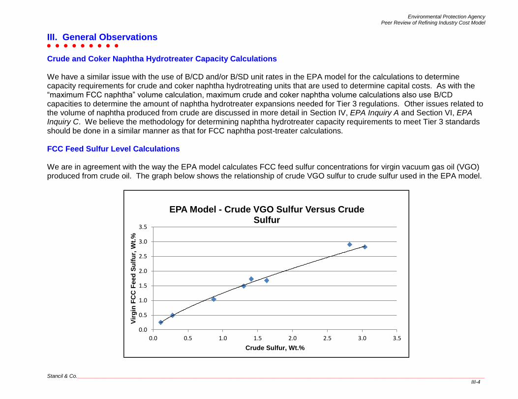
Crude and Coker Naphtha Hydrotreater Capacity Calculations We have a similar issue with the use of B/CD and/or B/SD unit rates in the EPA model for the calculations to determine capacity requirements for crude and coker naphtha hydrotreating units that are used to determine capital costs. As with the “maximum FCC naphtha” volume calculation, maximum crude and coker naphtha volume calculations also use B/CD capacities to determine the amount of naphtha hydrotreater expansions needed for Tier 3 regulations. Other issues related to the volume of naphtha produced from crude are discussed in more detail in Section IV, EPA Inquiry A and Section VI, EPA Inquiry C. We believe the methodology for determining naphtha hydrotreater capacity requirements to meet Tier 3 standards should be done in a similar manner as that for FCC naphtha post-treater calculations. FCC Feed Sulfur Level Calculations We are in agreement with the way the EPA model calculates FCC feed sulfur concentrations for virgin vacuum gas oil (VGO) produced from crude oil. The graph below shows the relationship of crude VGO sulfur to crude sulfur used in the EPA model.
0.0
0.5
1.0
1.5
2.0
2.5
3.0
3.5
0.0 0.5 1.0 1.5 2.0 2.5 3.0 3.5
Vir
gin
FC
C F
eed
Su
lfu
r, W
t.%
Crude Sulfur, Wt.%
EPA Model - Crude VGO Sulfur Versus Crude Sulfur

Environmental Protection Agency Peer Review of Refining Industry Cost Model
III. General Observations
Stancil & Co.____________________________________________________________________________________________________________________________________________ III-5
Data from Stancil’s crude assay database is shown on the graph below. While this graph represents more crude types with a wider range of sulfur concentrations, the general relationship yields crude VGO sulfur concentrations similar to the range of crude sulfur samples used in the EPA model.
There are, however, other gas oil streams produced in some refineries that are processed in the FCC unit that can add significantly to the sulfur load. These would include heavy gas oils produced from coker units, deasphalted oils produced from solvent deasphalting units, atmospheric residuum, and vacuum residuum. The most common stream is heavy gas oil produced from coker units. Coker heavy gas oil (HGO) yield is typically around 25 volume percent (Vol.%) of the vacuum residuum feed to a coker unit. The sulfur concentration of the coker HGO can roughly be estimated as about 1.1 times the sulfur concentration of the vacuum resid. The graph shown below represents the relationship of vacuum residuum sulfur to crude sulfur based on a vacuum residuum cut point of 1,000°F.
0.0
1.0
2.0
3.0
4.0
5.0
6.0
0.0 1.0 2.0 3.0 4.0 5.0 6.0
Vir
gin
FC
C F
ee
d S
ulf
ur,
Wt.
%
Crude Sulfur, Wt.%
Stancil - Crude VGO Sulfur Versus Crude Sulfur

Environmental Protection Agency Peer Review of Refining Industry Cost Model
III. General Observations
Stancil & Co.____________________________________________________________________________________________________________________________________________ III-6
Assuming a crude sulfur of 2.0 weight percent (Wt.%), vacuum residuum would contain about 4.0 Wt.% or 40,000 ppm sulfur. Coker HGO produced from this material would contain approximately 44,000 ppm sulfur. By comparison, virgin VGO produced from this same crude would have about 20,000 ppm sulfur. If the coker HGO comprised 10 Vol.% of FCC feed, the sulfur concentration would increase to 22,400 ppm, about 12% higher than a 100% virgin VGO feed.
Since FCC feed sulfur content is used to estimate FCC naphtha sulfur calculations in the EPA model that affect some of the logic used to determine post-treating technology choices, we think at a minimum the coker HGO should be included in the FCC feed sulfur calculations for those refineries with coker units.
y = -0.2093x2 + 2.3238x + 0.1941R² = 0.9316
0.0
1.0
2.0
3.0
4.0
5.0
6.0
7.0
8.0
0.0 1.0 2.0 3.0 4.0 5.0 6.0
Vacu
um
Resid
uu
m S
ulf
ur,
Wt.
%
Crude Sulfur, Wt.%
Stancil - Vacuum Residuum Sulfur Versus Crude Sulfur
Environmental Protection Agency Peer Review of Refining Industry Cost Model
IV. EPA Inquiry A
Stancil & Co.____________________________________________________________________________________________________________________________________________ IV-1
Inquiry A – Review the methodology for estimating the volume of light and heavy straight run naphtha which is based on a regression analysis of the API gravity and light straight run fraction from the assays of [13] crude oils. (This replaced the previous method of relying on similar correlation for the average quality of crude oil refined in each PADD).
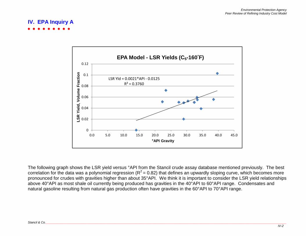
Initially, one concern we had for the methodology being used in the EPA model to determine crude naphtha yields is that the 13 crude oil assays used do not provide a large enough sample size to adequately develop generalized yield correlations with crude density in degrees American Petroleum Institute (°API) gravity for the various crude cut points in question. However, as Stancil will demonstrate with some examples, even with a larger sample size we are not convinced that the use of generalized yield equations will give accurate results for mixtures of various crudes types. While the 13 crude assays used in the EPA model provided some coverage of the crude types processed throughout the U.S. Stancil felt that a number of important crude types were left out of the mix. We did not see assays for shale oil (such as Bakken, Eagle Ford, etc.), heavy Canadian diluted bitumen crudes (such as Western Canadian Select (WCS), Cold Lake, etc.), or U.S. Gulf Coast (USGC) offshore crudes (such as Light Louisiana Sweet (LLS), Mars, Thunderhorse, etc.) represented. These crudes have been and will continue to comprise an increasing amount of the U.S. crude supply in the future. Based on our conversation during the kick-off meeting, it was our understanding that the number of crude assays available to the EPA for this study was limited, so we took the liberty of utilizing our crude assay database to develop some graphics to illustrate some of our concerns. Using the yield data from the 13 crude oils in the EPA model, we graphically recreated the yield representations for the crude light straight run (LSR) gasoline and heavy straight run (HSR) naphtha to visually illustrate the distribution of data. Each graph shows the linear equation that was developed from the data to estimate LSR and HSR yields as a function of °API gravity. We also developed similar graphs for LSR and HSR from a database of crude assays we maintain at Stancil. This data set contained approximately 175 different crudes that were recently updated. We recut the assays to the same distillation cut point temperatures as those in the EPA refining model. We note from the graph on the following page that the linear LSR yield correlation developed from the 13 crudes in the EPA model has a low coefficient of determination (denoted by R2) of 0.38 that is an indication the equation may have limited utility for producing precise results. Visually examining the data, one can conclude that the equation may produce reasonable yield results for crudes around 30°API (the median °API and LSR yield for all 13 crudes is 29.4 and 0.0506, respectively), but it is less clear how well it would predict LSR yields for crudes at 20°API or 40°API.
Environmental Protection Agency Peer Review of Refining Industry Cost Model
IV. EPA Inquiry A
Stancil & Co.____________________________________________________________________________________________________________________________________________ IV-2
The following graph shows the LSR yield versus °API from the Stancil crude assay database mentioned previously. The best correlation for the data was a polynomial regression (R2
= 0.82) that defines an upwardly sloping curve, which becomes more pronounced for crudes with gravities higher than about 35°API. We think it is important to consider the LSR yield relationships above 40°API as most shale oil currently being produced has gravities in the 40°API to 60°API range. Condensates and natural gasoline resulting from natural gas production often have gravities in the 60°API to 70°API range.
LSR Yld = 0.0021*API - 0.0125R² = 0.3760
0
0.02
0.04
0.06
0.08
0.1
0.12
0.0 5.0 10.0 15.0 20.0 25.0 30.0 35.0 40.0 45.0
LS
R Y
ield
, V
olu
me F
racti
on
API Gravity
EPA Model - LSR Yields (C5-160 F)

Environmental Protection Agency Peer Review of Refining Industry Cost Model
IV. EPA Inquiry A
Stancil & Co.____________________________________________________________________________________________________________________________________________ IV-3
Another part of this graph we would like to point out is in the gravity region around 20°API by noting there are several outlying data points with high LSR contents of 6 to 11 volume percent (Vol.%). These outliers are the heavy Canadian bitumen crudes that are diluted with natural gasoline, condensates, and light naphtha for transportation and handling requirements. The graph below is the linear HSR yield correlation developed from the 13 crudes in the EPA refining model. We note that the correlation has a reasonably good R2 value and visual examination indicates the equation has a reasonably good fit for the data provided.
y = 2E-06x3 - 8E-05x2 + 0.0022x + 0.0001R² = 0.8197
0.00
0.05
0.10
0.15
0.20
0.25
0.30
0.35
0.40
0.45
0.0 10.0 20.0 30.0 40.0 50.0 60.0 70.0 80.0
LS
R Y
ield
, V
olu
me
Fra
cti
on
API Gravity
Stancil - LSR Yield (C5-160 F)

Environmental Protection Agency Peer Review of Refining Industry Cost Model
IV. EPA Inquiry A
Stancil & Co.____________________________________________________________________________________________________________________________________________ IV-4
The following graph shows the HSR yield versus °API from the Stancil crude assay database mentioned previously. The best correlation for the HSR data was a polynomial regression with an R2 = 0.89 that defines an upwardly sloping curve similar to LSR, though less pronounced. As with LSR, we would reiterate the importance of considering the yield relationships above 40°API to account for shale oil, natural gasoline, and condensate production.
HSR Yld = 0.0090*API - 0.1063R² = 0.8827
0
0.05
0.1
0.15
0.2
0.25
0.3
0.0 5.0 10.0 15.0 20.0 25.0 30.0 35.0 40.0 45.0
HS
R Y
ield
, V
olu
me
Fra
cti
on
API Gravity
EPA Model - HSR Yields (160 F-350 F)
Environmental Protection Agency Peer Review of Refining Industry Cost Model
IV. EPA Inquiry A
Stancil & Co.____________________________________________________________________________________________________________________________________________ IV-5
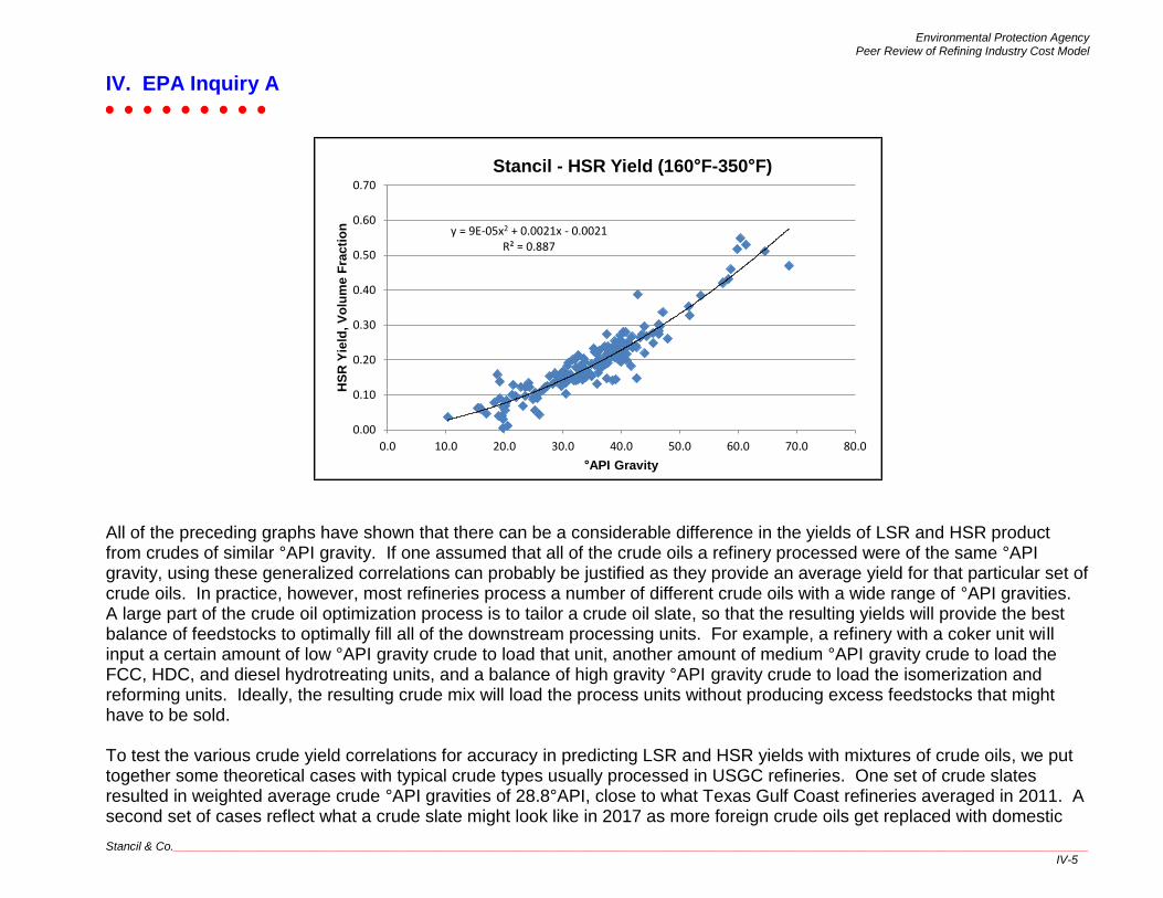
All of the preceding graphs have shown that there can be a considerable difference in the yields of LSR and HSR product from crudes of similar °API gravity. If one assumed that all of the crude oils a refinery processed were of the same °API gravity, using these generalized correlations can probably be justified as they provide an average yield for that particular set of crude oils. In practice, however, most refineries process a number of different crude oils with a wide range of °API gravities. A large part of the crude oil optimization process is to tailor a crude oil slate, so that the resulting yields will provide the best balance of feedstocks to optimally fill all of the downstream processing units. For example, a refinery with a coker unit will input a certain amount of low °API gravity crude to load that unit, another amount of medium °API gravity crude to load the FCC, HDC, and diesel hydrotreating units, and a balance of high gravity °API gravity crude to load the isomerization and reforming units. Ideally, the resulting crude mix will load the process units without producing excess feedstocks that might have to be sold.
To test the various crude yield correlations for accuracy in predicting LSR and HSR yields with mixtures of crude oils, we put together some theoretical cases with typical crude types usually processed in USGC refineries. One set of crude slates resulted in weighted average crude °API gravities of 28.8°API, close to what Texas Gulf Coast refineries averaged in 2011. A second set of cases reflect what a crude slate might look like in 2017 as more foreign crude oils get replaced with domestic
y = 9E-05x2 + 0.0021x - 0.0021R² = 0.887
0.00
0.10
0.20
0.30
0.40
0.50
0.60
0.70
0.0 10.0 20.0 30.0 40.0 50.0 60.0 70.0 80.0
HS
R Y
ield
, V
olu
me
Fra
cti
on
API Gravity
Stancil - HSR Yield (160 F-350 F)

Environmental Protection Agency Peer Review of Refining Industry Cost Model
IV. EPA Inquiry A
Stancil & Co.____________________________________________________________________________________________________________________________________________ IV-6
and Canadian grades. We should emphasize that these are not actual crude slates and are being used only for the purpose of assessing yield correlation accuracy. The first case, summarized below, uses crude data from the EPA refining model to calculate weighted averages for °API, LSR yield, and HSR yield based on the indicated percentages of Maya, Saudi Medium, Bonny Light, and West Texas Intermediate (WTI) crudes. We then used the EPA model equations to calculate LSR and HSR yields based on the weighted average crude °API. For this case, the EPA model equations under predicted both LSR and HSR by about 1.0% and 0.8%, respectively.
EPA Data - Conventional Crude 2011
% of Crude
Vol. Fraction
Crude Slate °API LSR HSR
Maya 45 22.3 0.0514 0.1252
Saudi Medium 25 30.4 0.0527 0.1504
Bonny Light 15 34.6 0.0389 0.1880
WTI 15 39.7 0.1028 0.2592
Weighted Average 100 28.8 0.0576 0.1610
EPA Equation Results 28.8 0.0479 0.1527
The second case with crude data from the EPA refining model is summarized below. For this case, we assumed Saudi Medium and Bonny Light are replaced with a mixture of Bow River and additional WTI. We allow a higher weighted average °API to reflect the abundance of light crude production expected in the future. For this case, the EPA model equations under predicted both LSR and HSR by about 2.7% and 1.4%, respectively.

Environmental Protection Agency Peer Review of Refining Industry Cost Model
IV. EPA Inquiry A
Stancil & Co.____________________________________________________________________________________________________________________________________________ IV-7
EPA Data - Conventional Crude 2017
% of Crude
Vol. Fraction
Crude Slate °API LSR HSR
Maya 35 22.3 0.0514 0.1252
Bow River 20 23.4 0.0719 0.1029
Bonny Light 0 34.6 0.0389 0.1880
WTI 45 39.7 0.1028 0.2592
Weighted Average 100 30.4 0.0786 0.1810
EPA Equation Results 30.4 0.0512 0.1669
The next set of cases used a number of different crude oils in the Stancil crude assay database to simulate the 2011 case and the Stancil LSR and HSR correlation equations discussed previously to estimate the LSR and HSR yields. For this case, a number of other crudes typically processed on the USGC (Bachaquero 17 (BCF-17), Mars, LLS, and Saharan Blend) were included. For this case, the Stancil equations prediction for LSR was very close, but the HSR prediction was low by about 2.9%.
Stancil Data - Conventional Crude 2011
% of Crude
Vol. Fraction
Crude Slate °API LSR HSR
BCF-17 15 16.9 0.0136 0.0456
Maya 20 21.6 0.0242 0.1292
Mars 10 29.0 0.0593 0.1521
Saudi Medium 22 30.8 0.0464 0.1833
Bonny Light 18 35.3 0.0543 0.2332
LLS 10 36.5 0.0550 0.1854
Saharan Blend 5 45.5 0.1309 0.2691
Weighted Average 100 28.8 0.0448 0.1622
Stancil Equation Results 28.8 0.0449 0.1331

Environmental Protection Agency Peer Review of Refining Industry Cost Model
IV. EPA Inquiry A
Stancil & Co.____________________________________________________________________________________________________________________________________________ IV-8
The final case with crude data from the Stancil database is summarized below. For this case, we assumed Saudi Medium, Saharan Blend and some BCF-17 are replaced with a mixture of WCS (diluted bitumen), WTI, and Eagle Ford Light (shale oil). As in the other future case, we allow a higher weighted average °API to reflect the abundance of light crude production expected in the future. For this case, the Stancil equations under predicted both LSR and HSR by about 0.6% and 2.9%, respectively.
Stancil Data - With Unconventional Crude
2017
% of Crude
Vol. Fraction
Crude Slate °API LSR HSR
BCF-17 10 16.9 0.0136 0.0456
Western Canadian Select 20 20.3 0.0624 0.0816
Maya 20 21.6 0.0242 0.1292
Mars 10 29.0 0.0593 0.1521
LLS 10 36.5 0.0550 0.1854
WTI 15 39.9 0.0718 0.2691
Eagle Ford Lt Shale 15 51.6 0.0917 0.3533
Weighted Average 100 30.3 0.0546 0.1738
Stancil Equation Results 30.3 0.0491 0.1445
Based on the information just presented, it is difficult to draw definitive conclusions for using the regression correlation method to estimate crude yields. For the case studies, all of the correlation equations tended to under predict LSR and HSR yields. Given the poor to mediocre R2 values for the correlation equations, we would expect there would be some fairly large margins of error in the predictions. The other trend of note from the case studies is the LSR and HSR prediction error tended to be larger for the future cases, which contained higher percentages of light crude and unconventional crudes. For the purposes of determining Tier 3 costs, under prediction of LSR and HSR could have the effect of underestimating the costs required for naphtha hydrotreating projects if more LSR needs to be hydrotreated. We would recommend that the EPA consider performing a sensitivity case assuming a 1% higher LSR yield to see what the impact would be on Tier 3 costs.

Environmental Protection Agency Peer Review of Refining Industry Cost Model
V. EPA Inquiry B
Stancil & Co.____________________________________________________________________________________________________________________________________________ V-1
Inquiry B – Review the methodology of basing the refinery blendstock volumes for the reformer, alkylation unit, isomerization unit, aromatics unit and naphtha hydrotreater on actual throughput volume data from the Office of Air Quality Planning and Standards (OAQPS). Alkylation unit throughput is reported as actual alkylate yield; therefore, using the actual alkylation throughput volumes from OAQPS will accurately reflect the blendstock volume in the gasoline pool. In the isomerization process, some hydrocracking reactions occur that result in some of the gasoline feedstock being converted to light gases. In our modeling work, Stancil generally assumes the isomerate blendstock yield is about 98.5 Vol.% of the unit throughput. The volume of reformate blendstock produced at the reformer will vary depending on feedstock quality, operating pressure, and the octane severity the unit is operating. The data shown in the “process inputs” sheet of the EPA model appears to indicate an operating severity of 90 research octane number (RON) across every PADD with an 87% reformate yield which would be consistent with a higher pressure, semi-regenerative catalytic reformer. There is a reformate yield chart in Petroleum Refining1 that matches this data for a feed quality with N+2A = 60 (N= Vol.% naphthenes, A= Vol.% aromatics). Following this curve shows the reformate yield effect for operating at higher severities. Continuous catalytic reformers (CCR) operate at lower pressures, which improve reformate yields. In our modeling work, Stancil generally assumes about 2.5 Vol.% improvement in reformate yields with a CCR unit. The table below summarizes the approximate yields, as discussed.
Semi-Regenerative Catalytic Reformer
Continuous Catalytic Reformer
Reformer Severity
(RON)
Reformate Yield
(Vol. %)
Reformate Yield
(Vol. %)
90 87.0 89.5
95 84.5 87.0
100 78.0 80.5
To attain the amount of reformate produced, the actual reformer throughput will need to be multiplied by the appropriate yield assumption in this table. For refiners making premium grade gasoline, reformers generally need to operate at a 97 RON to 99 RON severity for some amount of time to make a blending component with high enough octane to meet premium gasoline specifications of 91 to 93 road octane number. The rest of the time, they may only need to operate in the range of 92 RON to
1 James H. Gary and Glenn E. Handwerk, Petroleum Refining: Technology and Economics, 4
th ed., Marcel Dekker, Inc., New York, 2001, p. 202.

Environmental Protection Agency Peer Review of Refining Industry Cost Model
V. EPA Inquiry B
Stancil & Co.____________________________________________________________________________________________________________________________________________ V-2
95 RON as needed, to blend low octane components such as LSR, isomerate, light hydrocracker gasoline, light reformate, and raffinate. Refiners in the business of producing aromatics for petrochemical feedstocks may run their reformers at full rates and high severities all the time to maximize production of benzene, toluene, and xylene compounds. Also, some refiners that do not have on-site hydrogen production facilities or have access to off-site supplies of hydrogen may also run additional reformer throughput and severities to generate hydrogen for their desulfurization processes. In general, Stancil believes that assuming the reformate yields at 90 RON currently used in the EPA model may be overestimating the volume of reformate production. While we have no data to show what the average might be for the entire U.S., the refineries we work with on a routine basis typically operate in a range of 94 RON to 98 RON for semi-regenerative reformers and up to 100 RON for CCR units depending on their specific octane situation. Most of these refiners operating at the high end of the severity spectrum are undercutting reformer feed to distillates or blending reformer feed in gasoline. The refiners operating on the low end of the severity range tend to be more limited in their distillate operations and are reforming full range naphtha (i.e., 210°F to 380°F). Based on Stancil's view of reforming operations as described above, we would agree in principal with the concepts presented in the “Reformer Feed Logic” section in the MSAT2 representations of the EPA model for balancing reformer feed and overall gasoline volumes. Logically, we believe that shifting the 340°F to 400°F naphtha into jet fuel would be the first step to reducing reformer feed. The second step would then be to shift the 180°F to 285°F naphtha into gasoline blending or feedstock sales. Even so, it may not be reasonable to assume that refiners have enough excess octane in their pool to be able to blend large volumes of low octane 180°F to 285°F naphtha. We would recommend that EPA develop an octane balance for the gasoline pool to validate the assumptions for blending low octane reformer feedstock into gasoline. These octane balances would also shed some light on the appropriate reformer severity to assume for each refinery. In practice, refiners typically do not have a separate distillation tower to separate the reformer feed into 180°F to 285°F and 285°F to 340°F naphtha fractions. For the 180°F to 285°F naphtha fraction to be blended into gasoline or sold, it would need to be fractionated overhead with the LSR. For those refineries operating an LSR isomerization unit, cutting the LSR with a 285°F cut point could be problematic from a catalyst cycle length standpoint. Also, the cut point temperature between reformer feed and kerosene can range from as low as 300°F when operating in maximum kerosene mode to a high of 380°F when operating in maximum gasoline mode. Stancil has no data to indicate what the average HSR naphtha cut point is at this
Environmental Protection Agency Peer Review of Refining Industry Cost Model
V. EPA Inquiry B
Stancil & Co.____________________________________________________________________________________________________________________________________________ V-3
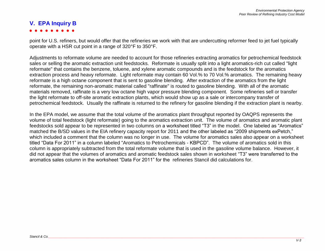
point for U.S. refiners, but would offer that the refineries we work with that are undercutting reformer feed to jet fuel typically operate with a HSR cut point in a range of 320°F to 350°F. Adjustments to reformate volume are needed to account for those refineries extracting aromatics for petrochemical feedstock sales or selling the aromatic extraction unit feedstocks. Reformate is usually split into a light aromatics-rich cut called "light reformate" that contains the benzene, toluene, and xylene aromatic compounds and is the feedstock for the aromatics extraction process and heavy reformate. Light reformate may contain 60 Vol.% to 70 Vol.% aromatics. The remaining heavy reformate is a high octane component that is sent to gasoline blending. After extraction of the aromatics from the light reformate, the remaining non-aromatic material called "raffinate" is routed to gasoline blending. With all of the aromatic materials removed, raffinate is a very low octane high vapor pressure blending component. Some refineries sell or transfer the light reformate to off-site aromatic extraction plants, which would show up as a sale or intercompany transfer of petrochemical feedstock. Usually the raffinate is returned to the refinery for gasoline blending if the extraction plant is nearby. In the EPA model, we assume that the total volume of the aromatics plant throughput reported by OAQPS represents the volume of total feedstock (light reformate) going to the aromatics extraction unit. The volume of aromatics and aromatic plant feedstocks sold appear to be represented in two columns on a worksheet titled “T3” in the model. One labeled as “Aromatics” matched the B/SD values in the EIA refinery capacity report for 2011 and the other labeled as “2009 shipments exPetch,” which included a comment that the column was no longer in use. The volume for aromatics sales also appear on a worksheet titled “Data For 2011” in a column labeled “Aromatics to Petrochemicals - KBPCD”. The volume of aromatics sold in this column is appropriately subtracted from the total reformate volume that is used in the gasoline volume balance. However, it did not appear that the volumes of aromatics and aromatic feedstock sales shown in worksheet “T3” were transferred to the aromatics sales column in the worksheet “Data For 2011” for the refineries Stancil did calculations for.

Environmental Protection Agency Peer Review of Refining Industry Cost Model
VI. EPA Inquiry C
Stancil & Co.____________________________________________________________________________________________________________________________________________ VI-1
Inquiry C – Comment on EPA incorporating, and how EPA incorporated in its refinery-by-refinery cost model, refiner plans for complying with the Mobile Source Air Toxics [MSAT2] rulemaking to reduce the content of benzene in their gasoline. This affected the volume of benzene precursors sent to the reformer or the volume of benzene extracted from the gasoline pool. We noted that the EPA model initially used a cut point temperature of 160°F for splitting LSR and HSR. For MSAT2 compliance, the EPA model later assumes the LSR cut point shifts up to 180°F to reduce the volume benzene and benzene precursors going to the reformer. In practice, we have found that many refiners operate their fractionators to a LSR cut point temperature of 200°F to 210°F for benzene control. While benzene and its precursor molecules boil in the range of 155°F to 180°F (shown in the table below), many fractionators used for splitting LSR and HSR simply do not have the number of trays and efficiency that would be needed to produce a sharp cut at 180°F that will remove most of the benzene and benzene precursors. As a result, there will be some benzene and benzene precursors that overlap into the higher boiling range fractions that diminish as the boiling range goes higher. Most compounds that boil in the 180°F to 200°F range do not have characteristics that make good reforming material, so there is little incentive to spend the capital or extra energy needed for recovery as reformer feed.
Compound Boiling Point, °F
n-Hexane 155
Methylcyclopentane 161
Benzene 176
Cyclohexane 177
Conversely, refiners in the business of aromatics recovery may operate below a 150°F cut point between LSR and HSR in order to maximize benzene production in their reformers. We noted that the EPA refining model was generating much more reformer feed for the total U.S. than was indicated by the actual reformer rates. After various adjustments in the model’s MSAT2 section, it appears that most of the 160°F to 180°F boiling range material was removed from reformer feed and routed to gasoline blending, isomerization, or sales. Expanding this MSAT2 cut point adjustment range to include the 180°F to 200°F fraction would directionally help reduce this reformer feed imbalance problem. The resulting increase in LSR production may also directionally increase the cost of compliance for the Tier 3 regulations.

Environmental Protection Agency Peer Review of Refining Industry Cost Model
VI. EPA Inquiry C
Stancil & Co.____________________________________________________________________________________________________________________________________________ VI-2
As mentioned in the previous section, final adjustments to reformate volume in the EPA model need to account for aromatics sales as petrochemical feedstocks as well as sales of light reformate that are used for off-site aromatic extraction plant feed. A benefit for refineries having these operations is that little else is needed to comply with MSAT2 regulations. For refineries utilizing isomerization or benzene saturation to control finished gasoline benzene levels, the reformate stream is also split, but the light reformate cut is only deep enough to capture the benzene. Typically, light reformate in this mode of operation has a cut point of 210°F to 220°F that allows the remaining heavy reformate to have benzene levels below 0.6 Vol.%. This very light reformate stream can be feedstock for the isomerization or benzene saturation units. The toluene and xylene materials remain in the heavy reformate fraction that goes on to gasoline blending. Light reformate has a low octane rating, generally in the range of 70 road octane number (RdON) to 75 RdON depending on benzene content. Saturating the benzene will generally lower the octane rating by 3 RdON to 4 RdON.

Environmental Protection Agency Peer Review of Refining Industry Cost Model
VII. EPA Inquiry D
Stancil & Co._____________________________________________________________________________________________________________________________________________ VII-1
Inquiry D – Review the methodology applied by EPA to estimate that refiners are maximizing propylene production at the expense of FCC naphtha production. Using refinery-by-refinery propylene sales information provided by EIA, EPA estimated that higher amounts of propylene production compared to the feedstock volume to the FCC unit would have caused lower FCC naphtha production. Propylene demand in the U.S. is about 15 million metric tons (MT) per year. The traditional sources of propylene have been naphtha-fed steam crackers that produce ethylene for the petrochemicals industry and FCC units at oil refineries. Together these sources supply about 90% of the propylene market. For both of these processes, propylene has historically been a by-product resulting from the production of the primary products these units were designed to make. The table below puts the demand for these various products into perspective.
Product
U.S. Demand
(Million MT/Year)
Propylene 15
Ethylene 129
Gasoline 26,600
Due to the low relative demand, propylene supply availability is generally more dependent on the demand for ethylene and gasoline than its own market. For example, if gasoline demand is high, refiners may increase run rates on their FCC units to produce more gasoline which also produces more propylene. Since propylene can also be used as feedstock for alkylation units, refiners might also choose to divert some propylene from sales to producing alkylate for gasoline blending or sales. Conversely, if demand for gasoline declines, refiners will cut FCC runs to reduce gasoline and consequently propylene drops as well. The graph below is a plot showing the average refinery production of propane and propylene by U.S. refiners since 1990. This data combines the volumes of propane with refinery-grade propylene (which is a usually an 80/20 mix of propylene/propane). As can be seen, refinery production of propane and refinery-grade propylene sales peaked between 2000 and 2004 and has been in a slight down trend since then, losing roughly 30,000 barrels per day (B/D) to 40,000 B/D on average.

Environmental Protection Agency Peer Review of Refining Industry Cost Model
VII. EPA Inquiry D
Stancil & Co._____________________________________________________________________________________________________________________________________________ VII-2
The next graph is a plot of the average refinery FCC unit charge over the same time period. FCC unit charge rates peaked around 2004 and were in decline until 2010 and have since appeared to stabilize. On average the decline has been around 400,000 B/D. Using a refinery-grade propylene yield of 11 Vol.% on FCC feed would translate into a production loss of 40,000 B/D to 45,000 B/D refinery-grade propylene. These charts do not indicate that refiners were taking any extraordinary measures to maximize propylene production beyond what they had been doing in the past.
350
400
450
500
550
600
650
19
90
19
91
19
92
19
93
19
94
19
95
19
96
19
97
19
98
19
99
20
00
20
01
20
02
20
03
20
04
20
05
20
06
20
07
20
08
20
09
20
10
20
11
20
12
Th
ou
san
ds
of
Ba
rre
ls P
er
Da
y
EIA - U.S. Refinery Production of Propane and Propylene

Environmental Protection Agency Peer Review of Refining Industry Cost Model
VII. EPA Inquiry D
Stancil & Co._____________________________________________________________________________________________________________________________________________ VII-3
The chart below shows refinery-grade propylene and unleaded gasoline prices on the USGC since 2009. As can be seen, refinery-grade propylene prices were very strong relative to gasoline from about mid-2009 through the summer of 2011. Based on the strength of these prices, we would opine that polypropylene producers may have bid up propylene prices to divert extra volume away from alkylation and gasoline production.
4200
4400
4600
4800
5000
5200
5400
5600
19
90
19
91
19
92
19
93
19
94
19
95
19
96
19
97
19
98
19
99
20
00
20
01
20
02
20
03
20
04
20
05
20
06
20
07
20
08
20
09
20
10
20
11
20
12
Th
ou
san
ds
of
Ba
rre
ls P
er
Da
y
EIA U.S. Fluid Catalytic Cracking Unit Charge
0
50
100
150
200
250
300
350
400
2009 2010 2011 2012 2013
US
GC
, C
en
ts P
er
Ga
llo
n
USGC Refinery-Grade Propylene and Unleaded Gasoline Prices
Refinery-Grade Propylene Unleaded 87

Environmental Protection Agency Peer Review of Refining Industry Cost Model
VII. EPA Inquiry D
Stancil & Co._____________________________________________________________________________________________________________________________________________ VII-4
The same trend is shown on the chart below which compares the prices of refinery-grade propylene with alkylate on the USGC. Since the end of 2011, propylene prices have been very volatile which would indicate supply and demand balance is very tight.
From the standpoint of the methodology used in the EPA refining model, we would agree that refiners were likely doing whatever they could to maximize propylene for sales for much of 2011 based on the strength in propylene prices. This would include adding ZSM-5 catalyst additive to their FCC units and diverting propylene feed away from alkylation to sales. For 2012 and 2013, the weaker price structure might have seen an on-again, off-again situation for maximizing propylene which in and of itself could have contributed to the price volatility. Refiners assess the economics for these operating decisions on a monthly basis and implementing either strategy is relatively easy to start and stop as economics dictate. ZSM-5 catalyst additive has been used in this manner for the last 25 years. Generally, we see base refinery-grade propylene yields of 10 Vol.% to 12 Vol.% on FCC feed without ZSM-5. Assuming a recovery factor of 0.85 would leave 8.5 Vol.% to 10 Vol.% for propylene sales. The EPA model is currently set up to activate the FCC naphtha to propylene volume shift at 6.5 Vol.%. We would recommend raising the activation level to at least 8.5 Vol.% if the EPA decides to continue using this shift.
0
50
100
150
200
250
300
350
400
2009 2010 2011 2012 2013
US
GC
, C
en
ts P
er
Ga
llo
n
USGC Refinery-Grade Propylene and Alkylate Prices
Refinery-Grade Propylene Alkylate

Environmental Protection Agency Peer Review of Refining Industry Cost Model
VII. EPA Inquiry D
Stancil & Co._____________________________________________________________________________________________________________________________________________ VII-5
Generally, each refiner has some maximum amount of ZSM-5 they can add to their FCCU that will allow them to capture some of the propylene and butylene yield benefits and still stay within the unit’s light ends handling capacities. Being a small market with unpredictable pricing margins would deter many refiners to expand this equipment for propylene alone. Those refiners situated near a petrochemicals complex that consumes propylene and could lock in long-term contract agreements would be more likely to upgrade their facilities to maximize propylene. For most of our modeling work, we have been using up to 5 weight percent (Wt.%) ZSM-5 concentration in FCC catalyst.

Environmental Protection Agency Peer Review of Refining Industry Cost Model
VIII. EPA Inquiry E
Stancil & Co._____________________________________________________________________________________________________________________________________________ VIII-1
Inquiry E – Comment on EPA’s methodology of forcing each refinery’s gasoline volume modeled by the refinery-by-refinery cost model to match actual refinery gasoline production volume as reported by refiners to EPA. In trying to match individual refinery gasoline volumes, we used the practice of undercutting FCC naphtha and heavy naphtha into the diesel and jet fuel pools. Since we often had mismatched gasoline volumes in those refineries with hydrocrackers, we also estimate hydrocracker operation (naphtha, intermediate, or diesel modes) as a means to match gasoline volumes. More often than not, heavy naphtha volumes tend to exceed reformer throughput volumes, so for those refineries that have excessive gasoline volumes, we assume that the excessive heavy naphtha volume is sold. For refineries with insufficient gasoline volume, this excess heavy naphtha volume is assumed to be blended into gasoline (but not reformed). In a couple of cases where there is a large shortfall in feedstock for reformers we assume that the heart cut of the FCC naphtha is being sent to the reformer for producing more aromatics for aromatics extraction. We agree that the technique used in the EPA model of undercutting heavy naphtha into jet fuel is a realistic way to balance both the reformer feed volumes as well as actual finished gasoline volumes to the model’s theoretical estimates. As mentioned in Section VI, EPA Inquiry C, we believe that light gasoline volumes (LSR, hydrocracker (HDC) light gasoline, and light coker gasoline) are likely understated with the cut points being assumed and are contributing some of the excess heavy naphtha reformer feed being predicted in the model. Undercutting heavy naphtha to the jet fuel or diesel pools is one of the easiest and most common steps refiners can take to shift gasoline to distillates. We also concur that the technique used in the EPA model of undercutting FCC naphtha into the diesel pool is another realistic way to balance gasoline volumes to the model’s theoretical estimates. In practice, refiners accomplish this by changing the cut point between naphtha and light cycle oil (LCO) at the FCC unit’s main fractionator. LCO is usually used as feedstock for the diesel hydrotreater (DHT) or HDC units. If a refiner is producing residual fuel oil, LCO may also be used as a blending stock to adjust density and viscosity specifications. While we agree that refiners have been directionally shifting HDC operations away from naphtha production to produce more distillates, it is difficult to generally categorize how much of a shift between naphtha and distillate mode a particular refinery is capable of. Determining the yields of naphtha or distillate a HDC will make depends largely on the type of feedstock, operating pressure, and catalyst type the unit is operating with. HDC feedstocks can be generally categorized as distillate, gas oil, and residual. Many older HDC units were originally designed to operate with distillate feedstocks in a boiling range of 600°F to 800°F such as diesel, atmospheric gas oil, light vacuum gas oil, and FCC LCO. LCO is typically limited to 25 Vol.% or 30 Vol.% of the total feed due to the amount of reaction heat it releases in an HDC. The hydrogenation reactions that occur in an HDC unit are exothermic, that is they release heat into the system, so maintaining control of the reactor temperature is a factor in

Environmental Protection Agency Peer Review of Refining Industry Cost Model
VIII. EPA Inquiry E
Stancil & Co._____________________________________________________________________________________________________________________________________________ VIII-2
considering feedstocks. Operating pressures on HDC units can range anywhere from 500 pounds per square inch gauge (psig) to 3,000 psig. Higher pressure will promote the hydrocracking reaction. The annual O&GJ World Refining Survey designates HDC units operating over 1,450 psig as being high pressure units. Many of the distillate HDC units listed in the O&GJ are considered to be high pressure conventional units. In a full conversion (naphtha) operating mode, a distillate feedstock HDC may yield 100% or more of gasoline boiling range material depending on the density of material used as feedstock. HDC units able to process heavy VGO as feedstock may be able to yield up to 108% gasoline range material in a full naphtha mode operation. With LPG recovery, HDC liquid yields can often be 120% to 130% of feed that result from cracking heavy materials into lighter materials and saturating them with hydrogen. HDC units operating in a maximum distillate mode usually operate with a different catalyst than those operating in a naphtha mode. Fractionating towers on many of the older HDC units were not designed with jet fuel or diesel draw trays or rundown lines and require installation of this equipment to operate in a distillate mode. In a full distillate operating mode, a distillate feedstock HDC may only yield 10% or less of gasoline boiling range material with distillate yields of 95% or more depending on the density of material used as feedstock. HDC units able to process heavy VGO as feedstock may yield 15% gasoline range material in full distillate mode operation. With LPG recovery, HDC liquid yields may only be 105% to 110% of feed. Losing 15% to 20% of liquid recovery volume can be a large disincentive for a refinery to operate in a full distillate mode. Refiners we are familiar with tend to operate in some intermediate mode between the two cases described. Some HDC units with heavy VGO feed operate at mild to moderate pressures (below 1,450 psig) and only partially convert the feedstock to gasoline and diesel products. The remaining unconverted material is processed by the FCC unit. This process is similar to an FCC feed treater. The difference is that instead of hydrotreating catalyst, hydrocracking catalyst is used. Some existing FCC feed hydrotreaters have been converted to this mode of operation. Yields of gasoline range boiling material for these units will be in the 10% to 15% range, distillate yields range from 30% to 35%, and 65% to 55% of hydrotreated FCC feed depending on the conversion. In summary, a lot of effort is spent in the EPA model to balance theoretical yields of gasoline against actual production volumes by shifting gasoline into distillates. Some of these are undercutting reformer feed into jet fuel, undercutting FCC naphtha into light cycle oil (LCO), and shifting hydrocracker (HDC) operations from naphtha mode into diesel mode. All of these are legitimate means that refiners use to shift gasoline production to jet fuel or diesel production. In the model, these shifts are done as needed to force the gasoline and reformer feed to balance with actual throughput and production values for each refinery though there is no data available to verify that a particular refiner is actually operating the way that the model assumes. One way the EPA could lend credence to the methodology would be to perform a distillate balance to see if the theoretical yields match actual data.

Environmental Protection Agency Peer Review of Refining Industry Cost Model
IX. EPA Inquiry F
Stancil & Co.____________________________________________________________________________________________________________________________________________ IX-1
Inquiry F – Review the new data received from vendors and how EPA is using that data. As suggested by the first peer reviewers, we requested and obtained more information from vendors of gasoline desulfurization equipment and included this information in the final rule cost analysis. The vendors confirmed that the hydrogen consumption values that they reported were actual, not stoichiometric. Vendor 1 Vendor 1 supplied inside battery limits (ISBL) capital and operating cost data for two different sets of cases where the initial FCC naphtha sulfur concentrations were assumed to be 2,000 ppm, 800 ppm, and 200 ppm. The basis for each of these cases was at 30,000 B/D and assumes each of these naphtha streams are treated down to 75 ppm sulfur with a single-stage reactor to represent the current Tier 2 FCC naphtha sulfur levels. The investment and operating cost data supplied for each case represents the incremental costs to further treat the FCC naphtha from 75 ppm to 25 ppm sulfur or from 75 ppm to 10 ppm sulfur. The first set of cases provided a wide array of minimum investment options for treating FCC naphtha from 75 ppm sulfur down to 25 ppm and 10 ppm by applying some undisclosed minor facility modifications and operating the existing single-stage reactor at more severe conditions to meet the 25 ppm and 10 ppm sulfur specifications. Most of these cases result in higher octane losses and shorter run lengths between catalyst change-outs. The vendor also indicated that in addition to additional catalyst costs and the associated maintenance, there would also be costs associated with storing untreated gasoline or shutting down the FCC unit. We would also add that shutting down or reducing rates significantly on the FCC would also be expected to curtail rates on virtually every unit in the refinery starting with the crude unit which produces most of the FCC feed and coker unit which receives its feed from the crude unit. Ideally, ancillary units like FCC naphtha hydrotreaters should be designed so the catalyst run length coincides with the normal turnaround schedules of the primary operating units (crude, FCC, coker, HDC, etc.) they serve. For an FCC unit, the turnaround cycle is usually four to five years. While we understand there may be some potentially new developments in technology and catalyst design that may improve the performance of existing FCC naphtha hydrotreaters, there was no information available in Vendor 1’s information package to evaluate the basis of these claims. Therefore, while these minimum investment cases are interesting, we are not convinced that they are practical from an operations standpoint. We noted the EPA incorporated some of this data in the refining cost model for evaluating FCC naphtha treating costs associated with the 10 ppm gasoline standard, but we were unable to follow how the vendor data might have been interpreted to get the investment requirements shown for the 200 ppm and 800 ppm cases. For the 200 ppm case, the EPA model shows $157.5 per B/D investment versus the vendor data that indicates a $0 investment for a 75 ppm to 25 ppm FCC naphtha sulfur

Environmental Protection Agency Peer Review of Refining Industry Cost Model
IX. EPA Inquiry F
Stancil & Co.____________________________________________________________________________________________________________________________________________ IX-2
reduction. Operating costs used in the model for this case matched the data supplied by the vendor. For the 800 ppm case, the EPA model shows $60 per B/D investment versus a range of $0 to $100 per B/D investment for a 75 ppm to 25 ppm FCC naphtha sulfur reduction. Operating costs used in the model for this case matched the data supplied by the vendor. We note that one of the first peer reviewers had similar concerns with the apparent inconsistency of investment requirements between the 200, 800, and 2,000 ppm cases in their 2011 report. If the EPA plans to use this minimum investment data, we would recommend that the additional costs associated with the FCC throughput reductions or shutdowns recommended by the vendor be included in the EPA model analysis. The second set of ISBL and operating cost data provided by Vendor 1 assumes installation of a second-stage reactor in the 800 ppm and 2,000 ppm sulfur FCC naphtha feed cases and a gasoline splitter on the 200 ppm sulfur FCC naphtha feed case. These cases applied primarily to reducing FCC naphtha sulfur to 10 ppm for the 5 ppm sulfur gasoline standard. All of this data for these cases was incorporated into the EPA model. Vendor 1 did include one case that added a second-stage reactor on an 800 ppm sulfur FCC naphtha feed case that reduced FCC naphtha from 75 ppm to 25 ppm for the 10 ppm gasoline standard but was not used in the EPA model. This seemed like a more reasonable case to use than the one chosen. Vendor 1 also provided ISBL capital and operating costs for installing a grassroots post-treater to reduce FCC naphtha from 100 ppm to 10 ppm sulfur to apply in situations where there is no existing FCC gasoline treater. We noted the EPA model also used this same capital cost data for the case to reduce FCC naphtha from 100 ppm to 25 ppm sulfur. The difference between the two cases was that the operating costs for the 25 ppm case were lowered proportionally from the 10 ppm case to reflect less sulfur removal. We noted that Vendor 1 did not give an accuracy assessment for the quotes given. Scoping type estimates such as these typically have +/- 30% to 50% accuracy, as Vendors 2 and 3 stipulated for their estimates. We note that the EPA model is currently set up not to include any capital cost contingency. We would recommend that the EPA consider adding at least a 30% capital cost contingency factor to the model. Vendor 1, however, did indicate outside battery limits (OSBL) costs to be 30% to 50% of ISBL investments versus the EPA model assumption of 35% of ISBL.

Environmental Protection Agency Peer Review of Refining Industry Cost Model
IX. EPA Inquiry F
Stancil & Co.____________________________________________________________________________________________________________________________________________ IX-3
Vendor 2 Vendor 2 supplied ISBL capital and operating cost data to upgrade existing units that are operating to reduce FCC naphtha sulfur concentrations of 800 ppm to 75 ppm. Two cost estimates were provided for installing a new polishing reactor to allow taking the treated FCC naphtha sulfur level from 75 ppm to 25 ppm and 75 ppm to 10 ppm. The ISBL capital costs in the EPA model for these two cases were consistent with the vendor estimates. The octane losses shown in the EPA model were somewhat higher than the vendor estimates. Vendor 2 provided estimates for hydrogen, fuel, and power consumption as a percentage increase over existing consumption, but did not give values for the existing consumption. Since the EPA model has data in per barrel consumption values for these items, we assume the EPA had access to the existing operating cost data. Since Vendor 2 did not supply cost estimates for either the 200 ppm or 2,000 ppm FCC feed sulfur cases, we assume the EPA applied some method to scale the 800 ppm FCC feed sulfur cost estimate up or down to generate the capital and operating cost estimates for the 200 ppm and 2,000 ppm FCC feed sulfur cases shown in the model. We were not able to readily discern how these adjustments were performed; however, the costs shown appeared to be directionally what we would expect. As mentioned previously, Vendor 2 indicated the accuracy of their capital cost estimates were +/- 50%. We would reiterate our recommendation that the EPA use a 30% contingency factor for capital cost estimates in the EPA model. Vendor 3 Vendor 3 supplied ISBL capital and operating cost information for both single-stage and two-stage FCC naphtha hydrotreaters processing FCC naphtha with sulfur levels of 800 ppm at 10,000 B/D. The single-stage cases provided the costs for reducing the FCC naphtha sulfur from 800 ppm to a base case level of 75 ppm and also to 10 ppm. The two-stage cases provided the costs of reducing the FCC naphtha sulfur from 800 ppm to a base case level of 25 ppm and also to 10 ppm. To estimate the costs for adding a second-stage reactor, the EPA subtracted the capital and operating costs for a two-stage unit from the costs of the base case single-stage unit (800 ppm to 75 ppm sulfur). This was done for both the 800 ppm to 25 ppm and the 800 ppm to 10 ppm two-stage reactor cases. The resulting differences in capital cost were multiplied by a vendor supplied factor of 1.15 to account for extra costs that might be incurred from adding the second reactor to an existing unit versus building a new two-stage unit from scratch. The resulting capital costs and operating costs for each of the new second-stage units appear to give reasonable results. We would still recommend that the EPA use the +/- 30% contingency factor provided by the vendor for capital cost estimates in the EPA model.

Environmental Protection Agency Peer Review of Refining Industry Cost Model
IX. EPA Inquiry F
Stancil & Co.____________________________________________________________________________________________________________________________________________ IX-4
We were able to validate Vendor 3’s cost estimate for building a two-stage unit based on the construction costs we have seen working with various clients and construction companies. Including the 30% contingency factor, Vendor 3’s cost estimates for building a two-stage FCC naphtha hydrotreater match fairly well with what our own cost curves would predict. While we do not have any cost curves for adding a second-stage reactor alone, the fact that we can match the vendor’s capital cost for a full two-stage unit allows us to have confidence in the method used by the EPA for estimating Vendor 3’s costs for the second-stage reactor.

Environmental Protection Agency Peer Review of Refining Industry Cost Model
X. EPA Inquiry G
Stancil & Co.____________________________________________________________________________________________________________________________________________ X-1
Inquiry G – Review the methodology EPA used to adjust desulfurization costs to account for cases when a refinery’s modeled desulfurization situation differed from the typical case for which the vendors provided us information. For example, for reducing a refinery’s gasoline sulfur from 30 ppm to 10 ppm, the refiner would typically need to reduce its FCC naphtha from 75 to 25 ppm. Depending on the amount of FCC naphtha blended into its gasoline, the amount of sulfur control that the refiner would need to achieve in its FCC naphtha would be larger or smaller than this. We linearly adjusted the desulfurization cost to account for the variances from a typical case. For cases where the total sulfur removed between the Tier 2 and the Tier 3 case was greater or lower, a factor was generated to account for the difference in sulfur removed. For example, if a refinery has an existing FCC naphtha post-treater and the total amount of FCC naphtha sulfur removed needed to be 55 ppm to meet the 10 ppm gasoline pool sulfur standard, but the amount of sulfur removed by the new treating equipment installed was based on 50 ppm (75 ppm to 25 ppm), a factor of 1.10 was calculated (55/50 = 1.10) and used to increase the amount of H2 consumption and increase the amount of octane loss to account for the additional costs to remove the extra sulfur. Using the same formula, if the amount of sulfur that needed to be removed was lower than 50 ppm, the factor would reduce the amount of hydrogen consumption and octane loss. We would concur that adjusting the H2 consumption and octane loss costs are appropriate. We would also agree that there is no need to adjust the fuel, power, and catalyst costs as these are small in comparison. Also, there is no need to adjust the capital as this cost is more sensitive to naphtha charge rate than to the amount of sulfur removal.

Environmental Protection Agency Peer Review of Refining Industry Cost Model
XI. EPA Inquiry H
Stancil & Co.____________________________________________________________________________________________________________________________________________ XI-1
Inquiry H – Review the methodology EPA used to adjust desulfurization costs to account for situations where the level of desulfurization increases above a certain point that causes the desulfurization cost to be increase[d] substantially in a nonlinear manner, thus the costs begin to increase exponentially. If we did not make this adjustment, we believe that we would be underestimating the cost for those refineries which must achieve a very high percentage of desulfurization. As it turned out, all five of the refineries we tracked calculations for in the model had FCC naphtha post-treaters and fit the example described in Section G. Stancil did note that the formula used to calculate the single-stage correction factor for desulfurization amounts higher than 96% was unusual as it multiplies fraction of sulfur removal above 96% by 3. We assume that this is the adjustment being made to correct the situation described in your inquiry. From what we could gather from the various default options in the model, it appears that for refineries with no existing FCC naphtha post-treating, the option is to use the capital cost and operating data for Vendor 1’s grassroots post-treater that was designed to reduce FCC naphtha from 100 ppm to 10 ppm sulfur. Since this hydrotreater is operating at level not much different than the second-stage polishing units estimated, the operating costs are fairly low versus what would be expected for a unit removing over 96% of the FCC naphtha sulfur. If over 96% of the sulfur is being removed to get to a 25 ppm target, the FCC naphtha feed would be over 600 ppm to 800 ppm sulfur. With this level of feed sulfur, the operating costs would look more like the grassroots single-stage hydrotreater estimates provided by Vendor 3 which are roughly three times higher than the operating costs for Vendor 1’s grassroots post-treater. If Vendor 3’s post-treater capital and operating cost data were used as the default option, then perhaps the single-stage correction factor above would not be needed. Otherwise, we would concur that multiplying the operating costs of Vendor 1’s 100 ppm to 10 ppm by 3 is an appropriate correction.

Environmental Protection Agency Peer Review of Refining Industry Cost Model
XII. EPA Inquiry I
Stancil & Co.____________________________________________________________________________________________________________________________________________ XII-1
Inquiry I – Review and comment on the conclusions that EPA reached through a conversation with technical experts that extractive treating of butane is widely practiced today by refiners and that the sulfur level of butane is under 5 ppm. Thus, no additional desulfurization needs to occur for butane. Also, between a review of crude oil assays and the follow-up discussion with technical experts, it was concluded that extractive treating of light straight run naphtha (LSR) from sweeter crude oils will yield a low sulfur level in that stream that would not require additional desulfurization under Tier 3. However, even after extractive treating of LSR from more sour crude oils, LSR could still contain greater than 10 ppm sulfur that refiners may find too high under Tier 3 (this assumes that the LSR is being blended straight to gasoline instead of being hydrotreated before being isomerized). Stancil would agree that extractive treating of butane is widely practiced today but not necessarily for the reason of lowering total sulfur in the product. Butane and other LPG products have copper strip corrosion specifications. Hydrogen sulfide (H2S) and other acidic compounds are the primary culprits that cause a failure of this test. Even 1 ppm H2S can result in a failed corrosion test. Refiners usually treat butane and other LPG products with caustic or amine compounds to extract the H2S and neutralize any acidic compounds. There are other sulfur compounds in butane called mercaptans that contribute to the total sulfur content of the stream, but do not affect the corrosion test. Since caustic treating will also remove mercaptans from butane, a consequence of meeting corrosion test specifications is that the butane will usually end up having lower total sulfur. Testing for free H2S at the 1 ppm level is difficult to do, so refiners sometimes measure the mercaptan level of the butane going and coming out of the caustic treater to assure some level of mercaptan reduction is taking place. Since H2S will be removed before the mercaptans, observing a reduction in the mercaptan levels across the treater will assure all of the H2S is removed. This does not, however, necessarily assure that an ultra low sulfur butane product is being produced. We have noted sulfur amounts in blending butane that range anywhere from 0 ppm to 30 ppm at the refineries we work with. We would also point out that specifications for storage of refinery-grade butane at Mount Belvieu, the largest underground LPG storage facility on the USGC, allows up to 140 ppm total sulfur. This is also the specification for physical butane that is used for settling futures contracts at the Chicago Mercantile Exchange (CME). Some LPG pipeline companies also have this same 140 ppm total sulfur while others have a 30 ppm total sulfur specification. In addition to butane that is produced at refineries, butane produced at NGL fractionation facilities is also stored at Mont Belvieu and may not be treated to the same sulfur level as at a refinery. Many refiners store excess butane production off-site during the summer months when gasoline RVP specifications are low and bring them back to the refinery for gasoline blending in the winter months when RVP specifications are higher. If they are storing the butane in a fungible storage facility like Mount Belvieu, the sulfur level of the butane they bring back from storage
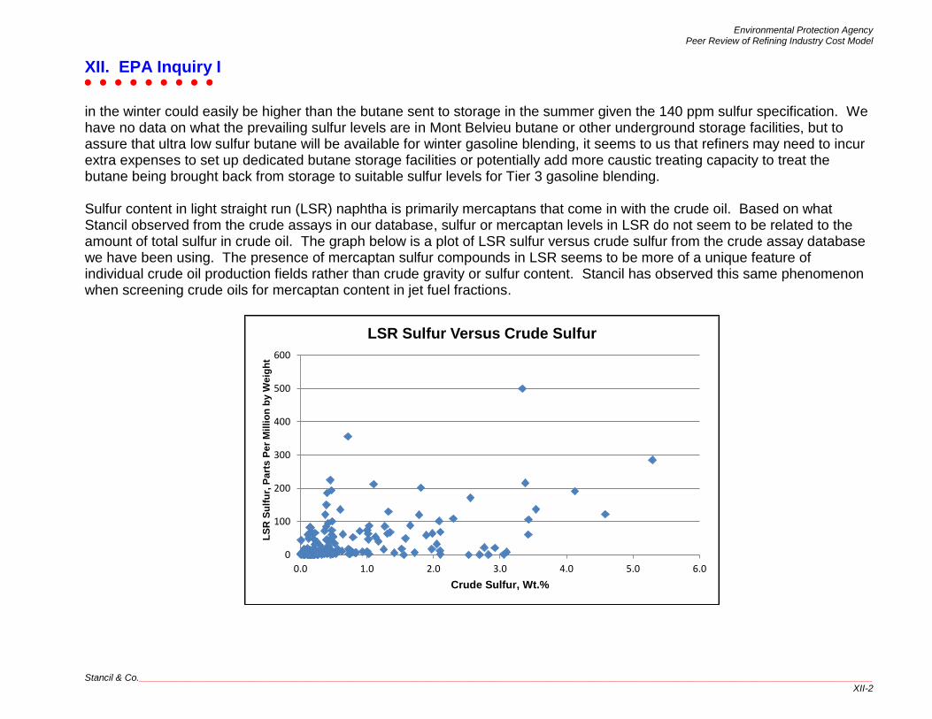
Environmental Protection Agency Peer Review of Refining Industry Cost Model
XII. EPA Inquiry I
Stancil & Co.____________________________________________________________________________________________________________________________________________ XII-2
in the winter could easily be higher than the butane sent to storage in the summer given the 140 ppm sulfur specification. We have no data on what the prevailing sulfur levels are in Mont Belvieu butane or other underground storage facilities, but to assure that ultra low sulfur butane will be available for winter gasoline blending, it seems to us that refiners may need to incur extra expenses to set up dedicated butane storage facilities or potentially add more caustic treating capacity to treat the butane being brought back from storage to suitable sulfur levels for Tier 3 gasoline blending. Sulfur content in light straight run (LSR) naphtha is primarily mercaptans that come in with the crude oil. Based on what Stancil observed from the crude assays in our database, sulfur or mercaptan levels in LSR do not seem to be related to the amount of total sulfur in crude oil. The graph below is a plot of LSR sulfur versus crude sulfur from the crude assay database we have been using. The presence of mercaptan sulfur compounds in LSR seems to be more of a unique feature of individual crude oil production fields rather than crude gravity or sulfur content. Stancil has observed this same phenomenon when screening crude oils for mercaptan content in jet fuel fractions.
0
100
200
300
400
500
600
0.0 1.0 2.0 3.0 4.0 5.0 6.0
LS
R S
ulf
ur,
Pa
rts
Pe
r M
illi
on
by W
eig
ht
Crude Sulfur, Wt.%
LSR Sulfur Versus Crude Sulfur

Environmental Protection Agency Peer Review of Refining Industry Cost Model
XII. EPA Inquiry I
Stancil & Co.____________________________________________________________________________________________________________________________________________ XII-3
Based on this, we would have to conclude that there is not a particular crude sulfur percentage cut off point where extractive caustic treatment of LSR would stop and hydrotreating would begin. The cut-off point in the EPA model is currently set at a crude sulfur content of 1.0 Wt.%. One possible issue with extractive caustic treatment of gasoline boiling range material is that sulfur removal efficiency is lower than for lighter LPG feedstocks. We have only anecdotal evidence from a competing vendor that this efficiency may be as low as 90%. At this efficiency level, LSR feed with sulfur concentrations over 10 ppm could become problematic if a refinery were depending on a treated LSR sulfur content of 1 ppm for gasoline blending as is in the EPA model. We would recommend that the EPA try to verify from vendors what the sulfur removal efficiency is for extractive caustic treatment of LSR materials. For those refineries that have coker units, the naphtha produced is usually processed with the LSR and HSR such that the light coker naphtha will end up combined with the LSR. Even with a light sweet crude slate, light coker naphtha can easily have 2,000 ppm to 3,000 ppm sulfur content. Considering the efficiency hurdle needed for extractive caustic treatment to be effective, we would recommend those refineries with coker units automatically default to installing new LSR hydrotreating capacity if needed.

Environmental Protection Agency Peer Review of Refining Industry Cost Model
XIII. EPA Inquiry J
Stancil & Co.____________________________________________________________________________________________________________________________________________ XIII-1
Inquiry J – Ensure the integrity of the new calculations (added since the first peer review) in the refinery-by-refinery cost model by working through those equations in the spreadsheet. Check the new equations with sufficient frequency (i.e., one refinery in each PADD) to ensure that the refinery model formulas refer to the appropriate cells. Report any errors. We tracked the calculations for five different refineries, one per PADD as requested, beginning with unit capacities to end with the final cost results. All of the equations appeared to calculate correctly and refer to the appropriate cells as far as we could tell. Chasing down the logic loops in the model through redundant capacity tables tended to made this task a very time consuming process. The refineries we chose had similar sulfur reduction strategies so we were not able to fully check out the calculations for some of the more unusual refinery situations, but did our best to understand the logic employed. We noted that one of the refineries we tracked did not show any alkylation rate in the actual throughput data supplied by the OAQPS even though that particular refinery has an alkylation unit. Perhaps, the data was not supplied or did not get entered at OAQPS, but it may point to a problem with substituting actual data for standard capacity data into the model. We would suggest the EPA compare this actual data with the capacity data listed in the EIA and O&GJ capacity reports for consistency.