Peer Discipline and the Strength of OrganizationsI

David K. Levine1, Salvatore Modica2

Abstract

Groups do not act as individuals - as Olson and other have emphasized: incentives within groupsmatter. Here we study internal group discipline through a model of costly peer punishment. Weinvestigate schemes that minimize the cost to a collusive group of enforcing particular actions, anduse the model to determine how the strength of the group - as measured, for example, by ability toraise funds to provide a public good - depends on the size of the group, the size of the prize, andthe heterogeneity of the group. We �nd that voluntary provisions models do not scale properly,while the peer discipline model does. The peer discipline model predicts that for a �xed size ofan auctioned (rival) prize the strength of the group is single-peaked - increasing when the groupis small then declining. The strength of the group also declines with heterogeneity. When groupscompete for transfers which one group may have to make in favor of another we �nd that smallgroups have an advantage over larger ones.JEL Classi�cation Numbers:

C72 - Noncooperative GamesD7 - Analysis of Collective Decision-MakingD72 - Political Processes: Rent-Seeking, Lobbying, Elections, Legislatures, and Voting Behavior

Keywords: Folk Theorem, Anti-Folk Theorem, Organization, Group

IFirst Version: November 26, 2012. We are especially grateful to Michele Boldrin, Michael Chwe, Drew Fudenberg,Zacharias Maniadis, Eric Maskin, Andy Postelwaite and seminar participants at the St. Louis Federal Reserve Bankand Venice Conference on Economic Theory. We are grateful to the EIEF, to NSF Grant SES-08-51315 and to theMIUR for �nancial support.

∗Corresponding author David K. Levine, 1 Brooking Dr., St. Louis, MO, USA 63130Email addresses: david@dklevine.com (David K. Levine), salvatore.modica@unipa.it (Salvatore Modica)

1Department of Economics, WUSTL2Università di Palermo

Preprint submitted to Mimeo: WUSTL September 14, 2013

1. Introduction

Groups do not act as individuals - as Olson [46] and others have emphasized incentives within

groups matter. Formal research is however rather scant on the topic, and as we report below most

papers dealing with groups do not explicitly deal with internal working of group discipline. Group

strength depends on a number of characteristics, including the size and cohesion of the group.

Here we study self-sustaining discipline through a model of costly peer punishment. We investigate

schemes that might be adopted by a collusive group to minimize the cost of enforcing actions -

e�ectively social norms - which are possibly not Nash equilibria, and use the model to determine

how the strength of the group - as measured, for example, by ability to raise funds to provide a

public good - depends on the size of the group, the size of the prize, and the heterogeneity of the

group.

Our model is one of an initial choice of action by group members in a base game followed

by an open-ended game of peer punishment. In the open-ended peer punishment games group

members repeatedly audit each other and determine punishments for violating the social norm

and the prescribed behavior in audits. While this does not describe the method used to provide

incentives in all groups at all times - for example, we do not consider dictatorship by a residual

claimant or organizations that monitor one another - the setting is an important one for many of

the groups studied by political economists. The essential feature is that groups members agree

that not punishing deviators can in turn be punished, a condition which has been found crucial

also in �eld work such as that conducted by Elinor Ostrom and reported for instance in Ostrom

[47] and Ostrom, Walker and Gardner [48]. From a conceptual point of view punishment cannot

have a de�nite end even if there are third party enforcement agencies. As Juvenal was aware in

the 2nd Century CE �Quis custodiet ipsos custodes?� - who will guard the guardians? Repeated

game theorists know the answer to that question: they must guard each other and for that to be

possible the game should not have a de�nite ending.

Several considerations point to a model of peer discipline. As argued by Dixit [17], using the

formal legal system is costly (in terms of money, time and uncertainty of outcomes) and requires

veri�able information which is not always available. Moreover:

• In many settings third party enforcement is not even feasible - for example, in the case of

criminal gangs, or collusive oligopolists concerned about anti-trust law. In other contexts the

underlying action that may be enforced through peer punishment may be membership in an

organization - for example, members of an interest group may through peer discipline encour-

age each other to pay dues and join a lobbying group. Contractual relations are irrelevant

where the action undertaken is signature of the contract itself.

• In some settings the activities encouraged through peer discipline may be inimical to the

ostensible interests of the organization. For example, a corrupt police force may collude to

protect corrupt law o�cers by a �code of silence� that for obvious reasons cannot easily be

enforced by third parties.

1

• Even if contracting enforced by third parties is possible, the writing and enforcing of contracts

is expensive - this is especially likely to be the case in a group with many people.3 Moreover,

contracts are not a magic wand. Somebody must determine whether or not the contract has

been violated and if legal sanctions are required, and somebody else must check that this

determination was made properly, especially if it is decided that no punishment is called for.

Hence, while contracts with third parties may reduce the cost to the group of enforcement,

it does not alleviate the need for peer discipline.

The type of scheme we study - group members who seamlessly monitor each other - is frequently

seen in practice. Besides the procedures observed by Ostrom in her work on common property

management, it is the type of enforcement mechanism used by modern internet groups such as

Wikipedia and Slashdot. It is also typical of how criminal organizations operate - failure to carry

out a punishment is itself a punishable o�ense in the typical codes of criminal conduct. By contrast

enforcement mechanisms that involve only a single round of punishment tend to be less e�ective:

in cases such as the Better Business Bureau - a single agency charged with monitoring business

behavior - we �nd numerous complaints about the organization.4

The calculation of equilibria of our setting is essentially based on the strongly symmetric com-

putation of Abreu, Pearce and Stachetti [1].5 When punishment is costly to the punisher the Nash

equilibria of the �base game� will also be equilibria of the punishment game in which the signals are

ignored and nobody ever punishes. But depending on the parameters of the cost of carrying out

and receiving punishments and the quality of information there can be other �more cooperative�

equilibria. We characterize equilibria of the peer-punishment game, and derive the implementation

that maximizes group utility. This gives rise to a simple expression for the �cost of peer punishment�

that can be used to analyze the e�ectiveness of groups.

The use of punishments and rewards to induce desired behavior over basic actions is not a

new idea. It is the basis of the e�ciency wage model, for example as described in Shapiro and

Stiglitz [52], and also the models of collusion proofness, for example, as described by La�ont [32].

Generally speaking, these models have not had costs associated with enforcement - in the e�ciency

wage model there is generally no punishment on the equilibrium path, while in the La�ont model

punishments and rewards take the form of transfer payments so that there is no net cost. In

practice however, there is punishment on the equilibrium path - as in La�ont - but practical forms

of punishment, such as exclusion, generally have a net cost associated with them. In our setup we

allow the possibility of costs on the equilibrium path, and in addition model the enforcement of �rst

3Li [38] appears to argue the opposite. However we rarely see large groups in lobbying organization bound togetherby contractual relationships, while for individual employment and business arrangements involving small numbers ofindividuals are typically contractual when contractual arrangements are feasible.

4The 17th century pirates constitute an interesting exception. Their decisions had to be taken quite swiftly, andto avoid abuses they had a balance of power whereby abuses of the captain were judged by the quartermaster. Ofcourse the matter ended up there, in at most two rounds of judgment.

5The highly structured nature of the game avoids the types of complications found in more general repeated gamesas described in Fudenberg Levine and Maskin [22] and Sugaya [54].

2

stage punishments through subsequent actual rounds of auditing rather than through commitment

to carry out punishments (or transfers).

To determine group e�ectiveness we analyze willingness to pay, �rst in a context where a single

group bids for a given prize. Empirical results on the relation between group size and strength in

this case are mixed, see the survey by Potters and Sloof [51]. The theory indicates that the results

di�er depending on the rivalry of the prize. Our main �ndings are the following:

• In the case where prizes are non-rival, so that all group members receive the full bene�t of

the prize, a group is stronger the larger it is.

• In the case of rival prizes, where each group member receives a proportional share of a prize

of �xed value, the insight of Olson [45] is true only up to a point. When the group is small,

willingness to pay increases with group size up to a threshold. Above this threshold size

willingness to pay decreases with group size.6

• Homogeneous groups are stronger than heterogeneous ones.

We then turn to the case of two groups of di�erent size that compete for transfers, as is typically

the case in the political arena. Modeling bids as second price auctions we �nd that:

• For a prize of �xed size and of equal value to both groups there is an �optimal� group size,

and the stronger group is the one �closer� to that size. Moreover, various ine�ciencies are

likely to emerge.

• When one of the groups - or the seller (a politician for example) - can take the initiative in

setting the size of the prize, small groups are stronger in that they will obtain transfers from

larger groups at low �political� cost, while large groups will opt out of the competition. When

the seller sets the agenda the large group is favored and the transfers to the seller are more

substantial. One interpretation of results such as Olson [45] who give evidence that small

groups are often successful in practice is that this is because they take the initiative.

The model also makes speci�c quantitative predictions - that can be examined, for example, using

the laboratory methods of Dal Bo [13].

There is of course a large literature on lobbying and other interest groups. Generally these

models have fallen into four categories. Some treat the strength of the group as a black box and

proceed with a working assumption, generally one in which strength decreases with size (Olson [45]

Becker [6], Becker [9]), or in the case of Acemoglu [2] that strength increases with group size for a

relatively small and a relatively large group.7 A second class of models treats collusive groups as

6Of course di�erent models may deliver di�erent predictions. Dixit [17], Chapter 3 for example considers a two-period model of bilateral trading where misbehavior by a given individual in the �rst random match can be punishedif her second partner knows that when the second match occurs. Assuming that this information is harder to comethe larger the group yields the result that larger groups are less capable of enforcing `fair' trade.

7This is consistent with our results, since we show that strength increases with size for a small group, and for arelatively large group, the opposition is small, and therefore weak. Acemoglu is also more focused on non-rival case,such as the National Ri�e Association - where our results indicate that strength increases with size.

3

individuals - e�ectively ignoring internal incentive constraints - and focuses instead on information

di�erences between the groups: examples are Nti [44], Persson and Tabellini [50], Kroszner and

Stratman [31] La�ont and Tirole [34], Austen Smith and Wright [4], Banks and Weingast [5],

Damania, Frederiksson and Mani [14], Green and La�ont [26], La�ont [33] and Di Porto, Persico

and Sahuguent [16]. Dixit, Grossman and Helpman [18] is similar, but allows the endogenous

possibility that groups either act non-collusively, or collusively as a single individual. A few papers

assume that leaders of the group can distribute bene�ts di�erentially (this may or may not be what

Olson [45] has in mind by �selective incentives�8) so that there is no public goods problem: see for

example Nitzan and Ueda [43] and Uhlaner [55]. Finally Pecorino [49] and Lohmann [39] treat the

problem of individual contribution within a group as a voluntary public goods contribution problem

- a problem which other authors often indicate informally they view as key. As we shall point out,

such a model does not behave very well in understanding the reason why groups of similar relative

size, but very di�erent absolute size (farmers in Belgium versus farmers in the United States) seem

to be similarly e�ective.

Finally, we should mention a paper that goes in the direction opposite of ours: in Mitra [42]

there is a �xed cost of forming a group - in contrast to our conclusion that there is a �xed cost per

person in the group - so the more people there are the easier it is to overcome the �xed cost.

In the next two sections we lay out the model and characterize feasible and optimal discipline

implementations. In section 4 we then apply the results to analyze the relation between group size,

heterogeneity and strength. In section 5 we turn to competing groups and agenda setting. Section

6 concludes.

2. The Discipline Model

There are N > 2 identical players i = 1, . . . , N in the group. We �rst describe the peer discipline

environment, in which group members monitor each other. Along the lines of Kandori [29]'s

information systems we allow for the self-referential nature of punishment equilibria by supposing

that the group plays a potentially unlimited number of rounds.

In the initial round - we call it round zero - group members choose primitive actions ai ∈ Arepresenting production decisions and the like. We let aR ∈ A denote the action of a representative

member of the group. By playing ai against aR player i gets payo�s u(ai, aR), and also generates

a binary good/bad signal zi0 ∈ {0, 1} where the probability of a bad signal 0 is π0(ai, aR).9

8Olson's concept is a bit slippery. He may have in mind people who are not in a group bene�ting from theactivity of the group - although this view of voluntary group participation runs somewhat counter to his notion ofwhat constitutes a group. He argues that the group should devise auxiliary services (free lawyers, insurance) which�selectively� bene�t only group members. It is not entirely clear why it would not be better to free ride on the groupand pay directly for the auxiliary services, unless the group has some cost advantage in providing those services. Inour setting members to not have the option of leaving the group - which is to say that they can not avoid beingpunished by group members. For example, farmers cannot avoid being shunned by neighboring farmers by refusingto join a farm association.

9Note that we do not specify what happens if more than one player deviates from a common action chosen bygroup members either for signal probabilities or for utility. As we will restrict attention to symmetric equilibria in

4

Following the primitive actions and the corresponding signals and utilities, a sequence of audit

rounds t = 1, 2, . . . commences. During these rounds players are matched in pairs as auditor i

and auditee j.10 These matches may be active or inactive. A player cannot audit himself, so if

i = j a match is inactive. Second, auditing is possible only if it is the �rst audit round or if in the

previous round the auditee was herself an auditor in an active match. Hence if the current auditee

was an auditor in an inactive match in the previous round, the current match is also inactive. The

remaining matches are active.

In round t ≥ 1 in an active match an auditor i assigned to audit member j observes the signal

zjt−1 ∈ {0, 1} of the behavior of the auditee in the previous round and has two choices ri: to

recommend punishment (ri = 1) or not to recommend punishment (ri = 0), while the auditee j

does not get a move. Based on a member i's behavior as an auditor, another signal zit ∈ {0, 1}is generated. If the auditor recommends punishment on a bad signal or does not recommend

punishment on a good signal, then the bad signal is generated with probability π; otherwise with

probability πp ≥ π.Note that the consequences of auditing decisions are assumed to be symmetric in the sense that

π = Pr(zit = 0 | zjt−1 = 1, ri = 0) = Pr(zit = 0 | zjt−1 = 0, ri = 1), similarly with πp. We refer to

this as signal symmetry. In other words the distribution of zit depends only on whether the player

�follows the social norm� (punish on bad signal or not punish on good) but not on which right thing

she does. We should also mention that neither π0(ai, aR) nor π and πp depend on the size of the

group - in other words we assume that auditors are close to the auditees regardless of size.11

Remark. What is important is not what is true but what players think. Even if signal symmetryfails, it will be di�cult for players to learn the consequences of the asymmetry. If their learningprocess merges information about the particular way in which the social norm was followed, theywill act as if the distribution is symmetric. This can be formalized as the model of analogy basedexpectations developed in Jehiel [28]. Hence a broader interpretation of this assumption is that weare studying an analogy based equilibrium in which players do not distinguish di�erent deviationsfrom the social norm.

2.1. Costs and Punishments

Payo�s are additively separable between the initial primitive utilities and costs incurred or

imposed during auditing - that is, we assume quasi-linearity. There is no discounting, as we imagine

these rounds take place relatively quickly.

Following a recommendation of punishment a punishment is imposed, once or several times

with some probability. Suppose that the auditor is i. The corresponding auditee then su�ers an

expected utility penalty of P it ≥ 0, the auditor incurs an expected utility cost of Cit = θP it , and

which all group members play the same way, we only need to specify the pair (ai, aR) for determining equilibrium,so for notational simplicity and because it does not matter, we do not give a complete speci�cation of the game.

10We do not have in mind that only a single person assesses whether the auditee has adhered to the social norm,rather that there is a single auditor who evaluates the evidence, possibly provided by many other people, and makesa determination of �guilt� or �innocence.�

11This picture of localized monitoring is di�erent in spirit from Dixit [17], which in terms of our model may beinterpreted as arguing that the di�erences π0(ai, aR) − π0(aR) and πp − π decrease with group size.

5

in addition the other N − 2 members of the group share an expected utility cost of CiGt = ψP it .12

We assume that it is feasible to choose any value of P it , but that the corresponding costs to the

auditor and other group members are scaled accordingly, that is that θ and ψ are constants. We

refer to this as a linear punishment scheme. It includes the case in which there is one particular

punishment that may be repeated several times,13 possibly randomly: for example a coin can be

�ipped so that with some probability the player is punished twice. The scheme is also consistent

with the possibility of actual punishment being possible only once: for example losing a job or the

death penalty. In this case P it can be a probability (or �demerits�) that is cumulated over time,

with the actual punishment being issued at the time the game ends. Notice that it makes sense for

probabilities of indivisible punishments that utility is additively separable.

With the exception of the auditee whose loss must be non-negative, the other costs may be

either positive or negative, allowing the possibility that particular individuals may bene�t from the

punishment - for example if the auditee is demoted, some other group member may be promoted

to �ll the vacated position. However, we assume that the group as a whole cannot bene�t from

punishment, so that 1 + θ + ψ ≥ 0.

Discussion. Punishment may have many possible forms. For example, if the auditee is �red

from his job, removed from the organization or demoted this may have an adverse e�ect on the

organization and hence lower the utility of those group members who are not directly involved

in the punishment. On the other hand, some punishments may involve the collaboration of the

entire group - for example shunning or refusing to speak to a group member. These costs are in

a sense �avoidable� by an individual group member who may refuse to go along with the �social

norm� of carrying out the punishment, and so avoid the cost of doing so. Rather than giving each

player several decisions: whether to punish in a particular audit and also whether to carrying out

their own �share� of a punishment, we compress the decision into a single decision �whether to

follow the social norm.� Roughly speaking then we regard the individual cost Cit as including the

expected costs imposed by carrying out the player's individual share of punishments mandated in

other matches as well as their own.

There are two speci�c limitations with linear punishment schemes. First, there may be more

than one di�erent type of punishment: for example you may either be �red or moved to a less nice

o�ce. These di�erent punishments may have di�erent values of θ, ψ. However, if multiple values

of θ, ψ are available, after applying our results on group cost minimization for each value of θ, ψ

we may then pick the combination of θ, ψ that yields the least cost. Second, the linear punishment

schemes does not recognize that there may be an upper bound on the worst possible punishment.

Earlier literature, such as work on e�ciency wage, has focused on a higher level of informational

perfection and the size of the upper bound. As a practical matter, the fact that the worst possible

12There may also be a utility cost to individuals outside the group, however as this plays no role in analyzingequilibrium we ignore it for the time being.

13Since we assume that a player can potentially be punished in each round, it makes sense that he can be punishedseveral times in one round.

6

punishments that are used have diminished over time - at one time private organizations could

use torture as a punishment; now torture is usually banned, and in many cases even governments

are prohibited from using the death penalty, while private organizations are severely limited in

the punishments that they can carry out - suggests that extreme punishments are generally not

required to provide adequate incentives. Moreover, the set of applications we have in mind, such as

membership or contributions to lobbying organizations, or the decision whether to accept a single

bribe, generally do not bring great bene�ts or cost to the individual, so that large punishments are

not generally relevant. Hence our focus not on worst possible punishments, but rather the costs to

punisher and the group of carrying out the punishments - that is on the ratios θ, ψ rather than the

maximum levels.

There are two other limitations of the model. First, it allows only punishments and not rewards,

and second it does not allow for a �xed cost of carrying out an audit. This is primarily for simplicity.

The use of rewards and not punishments is essentially a normalization. If it is possible to reward

group members for good behavior, we can attribute the expected value of receiving a reward in every

audit round to the initial utility u(ai, aR), and consider not receiving the reward as a �punishment�

in subsequent rounds. Take the example of an end of year bonus that might be withheld. We can

on the one hand consider this as a reward. But we can equally well consider it part of income, and

treat the withholding of the bonus as a punishment.

Fixed costs of carrying on audits is more complex because these costs can potentially be avoided

by not carrying out the audit, and we need to consider how easy this is to observe. Our view is that

it is relatively easy to see whether an audit has been conducted, and relatively more di�cult to see if

it has been done with due diligence, so we focus on strategic misrepresentation of recommendations

rather than failing to carry out audits. If auditing is perfectly observable, then there is no cost in

equilibrium of carrying out punishments since they are o� the equilibrium path only, and we may

ignore the incentive e�ects of avoiding the �xed cost of auditing. Although our computations of

audit costs ignore �xed costs we may easily incorporate them into the model: if CF is the �xed cost

of carrying out an audit, since on the equilibrium path punishments are carried out with probability

π we may simply add CF /π to the group cost CG and this gives the correct expected cost of the

audit.14

2.2. Implementations and Equilibrium

An implementation speci�es the procedure for matching and a pro�le of punishment costs. At

the beginning of each audit round either the game ends or a matching and punishment pro�le are

established. A matching is simply a 1-1 map from the set of players to the set of players with

the argument being the auditor and the image being the auditee. A punishment pro�le is the

assignment of P i (and implicitly Ci = θP i, CiG = ψP i) to each auditor i's match.

14Notice that in this case if punishments are to be randomized it should be done by randomizing the audit itselfrather than randomizing following the recommendation - the former leads to a proportionate reduction of the �xedcost, the latter does not.

7

An implementation is a determination at the beginning of each round whether the game ends,

and if not of a matching and punishment pro�le. That determination can depend (randomly) on

the history of previous matchings and punishment pro�les. However it may not depend on the

private signals or past recommendations of punishments.

A pure strategy for a player is an initial action and subsequently choices of signal dependent

punishment recommendations. In general these choices depend both on the private history of the

player (the signals he has seen and the recommendations he has made) as well as the public history,

that is previous matchings and punishment pro�les. A pro�le of strategies are a Nash Equilibrium

if given the strategies of the others no player can improve his payo�. A public strategy depends only

on the public history and a perfect public equilibrium is a Nash equilibrium in public strategies with

the additional property that following every public history the strategies are a Nash equilibrium

in the subsequent game. A peer discipline equilibrium is a perfect public equilibrium in which all

players follow the strategy of punishing on the bad signal and not punishing on the good signal,

and we say that we say that aR is incentive compatible in the implementation if there is a peer

discipline equilibrium with aR as common initial action.

Note that the rules of the implementation are not strategically manipulable in the sense that

future matching and punishment pro�les do not depend on the recommendations made by auditors

- the chances of future participation are exogenous, and an auditor need only care about the chances

of being audited and punished in the next round.

An obvious and important fact is that a possible implementation is not to have any auditing

rounds. In this case aR is incentive compatible in the implementation if and only if it is a symmetric

Nash equilibrium of the primitive game with payo�s u(ai, aR). Our interest will be in establishing

which non-Nash outcomes in the primitive game can be sustained by non-trivial peer punishment

- and at what cost.

We should note that in the general case there is no assumption of anonymity and players may

be treated di�erently based on their name. Indeed, it may be that some people are audited less

frequently than others, so must be punished more when �caught.� Or it may be that only a subset

of the population carry out audits - or that there is a hierarchy, with only �managers� conducting

audits, and only a subset of �top managers� conducting audits in the next round, and so forth.15

2.3. Enforceability

Recall that in the initial primitive round the probability of a �bad� signal 0 is π0(ai, aR) and

utility is u(ai, aR). Following the repeated game literature such as Fudenberg Levine and Maskin

[22] we say that aR is enforceable if there is some punishment scheme based on the signal such

15While we consider groups that collude to minimize costs to the group of punishment, we do not impose renegoti-ation proofness. In the case of groups that collude by communication in setting up rules, it is typically expensive andimpractical to convene a meeting every time a decision must be made. We imagine that such meetings are infrequentrelative to the frequency with which decisions are taken. Moreover, in some cases the equilibrium and mechanism thatminimizes cost may evolve rather than be explicitly agreed to, or agreed to at a far distant time, possibly by peoplequite di�erent from those currently in the group. These tendencies are strengthened in light of evidence showing thatthere is strong inertia in Nash equilibrium when many people are involved.

8

that aR is incentive compatible. In the case of a binary signal, this means there must be some

punishment P1 such that for all ai we have u(aR, aR)− π0(aR, aR)P1 ≥ u(ai, aR)− π0(ai, aR)P1. If

for all ai we have u(ai, aR)− u(aR, aR) ≤ 0 we say that aR is static Nash. This case is not terribly

interesting since no peer discipline is required to implement it as an outcome.

We now characterize enforceability. Let σ(ai, aR) ≡ sgn(π0(ai, aR)−π0(aR, aR)). For σ(ai, aR) =

0, that is for actions indistinguishable from aR, if u(ai, aR) = u(aR, aR) de�ne the gain function

G(ai, aR) = 0, otherwise G(ai, aR) = sgn(u(ai, aR) − u(aR, aR)) · ∞. For actions that are distin-

guishable from aR de�ne the gain function to be

G(ai, aR) =u(ai, aR)− u(aR, aR)

π0(ai, aR)− π0(aR, aR).

Let nowG(aR) ≡ maxσ(ai,aR)≥0 G(ai, aR) andG−(aR) ≡ minσ(ai,aR)<0 G(ai, aR). Note thatG−(aR) ≥0 if and only if σ(ai, aR) ≥ 0 for all ai with u(ai, aR)− u(aR, aR) > 0.

Lemma 1. The group action aR is enforceable with the punishment P1 ≥ 0 if and only if max{0, G(aR)} ≤P1 ≤ G−(aR), hence it is enforceable if and only if max{0, G(aR)} ≤ G−(aR).

Proof. Spelling out the inequality u(aR, aR)−π0(aR, aR)P1 ≥ u(ai, aR)−π0(ai, aR)P1 and applyingthe de�nitions just given yields that aR is enforceable with punishment P1 ≥ 0 if and only ifmax{0, G(aR)} ≤ P1 ≤ G−(aR). The conclusion follows.

Observe that enforceability only concerns the �rst audit round hence does not imply peer

discipline in the full sequence of audit rounds: an agent will deviate from an enforceable aR if she

thinks that punishment will not be in�icted in the future. For peer discipline equilibrium we need

more.

3. Feasible and Optimal Implementations

We �rst examine the simple case of a two-stage implementation. This both serves to illustrate

how the model works, and, as we shall see, as far as optimality goes, is perfectly general. In

the two stage implementation a single punishment level P1 is chosen along with a probability of

continuing the game after each audit round 0 < δ < 1. When audit rounds take place, matchings

are symmetric: for example we may place players randomly on the circle and have each player audit

the adjacent opponent in the clockwise direction.

3.1. Characterization of Equilibrium in the Two-Stage Implementation

For notational simplicity, we set πR0 = π0(aR, aR), GR = G(aR), uR = u(aR, aR).

Theorem 1. If the action aR is not static Nash it can be incentive compatible in the two-stageimplementation only if aR is enforceable and P1 ≥ max{GR, |θP 1|/[πp − π]}. In this case, aR isincentive compatible if and only if

P1 ≥ GR , δ ≥ |θ|/[πp − π].

9

The resulting equilibrium utility level is

uR −[πR0 + (δ/(1− δ))π

](1 + θ + ψ)P1.

Proof. Recall that in the present case punishment is in�icted only if the game continues, whichoccurs with probability one in the initial round and δ in the other ones. The condition P1 ≥ GR

thus follows from Lemma 1.In an audit round, if you are an auditor and see a bad signal you are willing to punish if and

only if the cost you would save by deviating is no greater than the extra expected punishment youwould get next round, that is C1 ≤ δ[πp − π]P1, or θ ≤ δ[πp − π]. Similarly, if you are an auditorand see a good signal you are willing not to punish if and only if θ ≥ −δ[πp − π]. Combining thesetwo gives the second incentive constraint.

The necessary conditions follow from δ ≤ 1. The expected present values on the equilibrium pathare then computed by summing the geometric series given the parameters. Indeed the individualplayer gets θP1 as an auditor and P1 as an auditee, each in the event of a bad signal; the groupcost term is ψP1, equal to ψP1/(N − 2) times the number of times it is incurred which is N − 2(the audits where the player does not participate).

Notice that equilibrium utility for group members goes to minus in�nity as δ → 1: this is

because punishment occur essentially forever - it can be viewed as a kind of Hat�eld and McCoy

equilibrium.16

3.2. Optimal Punishment Plans in the Two-stage Case

We now consider choosing P1, δ to maximize the utility of a representative group member for a

given initial action aR. The condition P1 ≥ max{GR, |C1|/[πp − π]} is maintained.

Theorem 2. The non static-Nash enforceable initial action aR is incentive compatible for sometwo-stage implementation if and only if |θ| < πp−π. In this case to maximize the average expectedutility of the group over two-stage implementations it is necessary and su�cient that the incentiveconstraints hold with equality, that is

P1 = GR , δ =|θ|

πp − π

The equilibrium utility level is

uR −[πR0 +

|θ|[πp − π]− |θ|

π

](1 + θ + ψ)GR.

Proof. From Theorem 1 the objective is decreasing in both P1, δ hence it is maximized when theseparameters are minimized - that is, when the constraints bind.

Remark. Observe that we can always increase the δ's slightly and obtain an equilibrium that isstrict in all the audit rounds at the price of a small reduction in group welfare. Such an equilibrium

16Notice also that if 1 + θ + ψ > 0 and θ, ψ > 0 these equilibria are not renegotiation proof - in this case allgroup members will prefer that the punishments not be carried out. If either θ or ψ are negative then after therecommendations are made at least some group members will wish to carry out the punishments, while before thesignals are seen all will agree to dispense with auditing rounds. See also footnote 15.

10

can be more robust as it does not require individuals to �make the right choice� when indi�erent.Notice however that, as we shall see below, it is not always possible to avoid indi�erence in the �rstperiod.

3.3. The General Linear Case

Theorem 2 in fact holds not only for all two-stage implementation, but as shown in the Appendix,

for all implementations.

Theorem 3. The non static-Nash enforceable initial action aR is incentive compatible for someimplementation if and only if |θ| < πp − π. In this case to maximize the per capita expected utilityof the group it is necessary and su�cient that the incentive constraints hold with equality for eachpositive probability public history. The per capita expected equilibrium utility level per person is

uR −[πR0 +

|θ|[πp − π]− |θ|

π

](θ + ψ + 1)GR.

The expression

Π ≡[

|θ|[πp − π]− |θ|

π

]can be viewed as a measure of the frequency of peer punishment on the equilibrium path, and we

can rewrite per capita group utility as

uR − (πR0 + Π)(θ + ψ + 1)GR.

Notice that even if θ is zero, there is still a cost[πR0 (ψ + 1)

]GR from the need to punish in the

�rst round.

4. Group Size and the Strength of Groups

What determines strength of a group? A simple measure of group e�ectiveness is its ability

to mobilize resources. In this section we analyze a simple model of willingness to pay and focus

particularly on the role of group size in determining strength. This group e�ectiveness can have a

variety of interpretations - for example the group might be attempting to corrupt a politician as in

Ades and DiTella [3] or Slinko and Yakovlev [53], or it could be a consortium bidding on a contract.

Throughout this analysis we will maintain the assumption that |θ| < πp − π so that peer

punishment is feasible. We study simple model of linear cost of e�ort and a prize worth S that

will be divided equally among the group, each group member getting a bene�t of s = S/N . The

question we ask is: how much e�ort is the group willing to provide to get the prize? To determine

willingness to provide e�ort, we use a Becker-DeGroot-Marschak (BDM) elicitation procedure.17

The bid itself is a commitment to an implementation and basic actions that are incentive compatible

with respect to that implementation; this includes also the possibility of not using peer discipline

17Basically this is a second price auction. In the political economy setting the all-pay auction studied, for example,by Krishna and Morgan [30] may be more relevant, but here we are trying to abstract from strategic considerations.

11

at all, but having instead (incentive compatible) voluntary contributions. E�ort is provided only

after the bid is accepted; otherwise the situation would be strategically one of an all-pay auction.

Hence we have in mind a lobbyist who goes to a politician and says �my group will provide so many

campaign contributions and provide so many volunteers in your next election if you provide us with

S.� We will consider also the case in which the prize can be rescinded if a threshold e�ort level is

not provided.

E�ort may be divisible or indivisible. Strategically this makes a di�erence: when e�ort is divis-

ible, everyone can contribute equally a small amount, and it is relatively easy to monitor whether

individuals made the agreed upon contribution. As a practical matter e�ort is not indivisible: lob-

bying, protesting, bribing and so forth require an overhead cost of thinking about and organizing

oneself to participate in the activities. In general it is not feasible to spend two minutes a year

contributing to a group e�ort in an e�ective way. Hence we will focus on the case where each group

member j can provide either 0 or 1 unit of e�ort: ej ∈ {0, 1}.With indivisible e�ort in order to bid B the group should appoint a subset of B members each

to provide an e�ort level of 1. To maintain symmetry of e�ort provision across group members we

assume this is done through a messaging technology by which the group sends messages to individ-

uals indicating whether they are expected to contribute: each individual j receives an independent

signal σj = {0, 1} of whether or not to provide e�ort, where µ ≡ pr(σj = 1) = B/N . Notice that

the actual e�ort level that will be provided is random - however the bid is evaluated according to

the expected value. The BDM mechanism chooses a random number B and if B ≤ B the bid is

accepted. For reasons that will emerge below - groups may prefer a higher e�ort level to a lower

one - when the bid is accepted we take B to be a �oor on e�ort - the group is free to deliver a

higher level if it chooses to do so. To model imperfect monitoring we assume that auditors can

tell whether or not the auditee has contributed e�ort, but observe whether or not they received a

signal with noise. That is, it is observable whether or not the auditee turned up at the rally, but if

he did not, he may say �I never got the phone call� and the auditor cannot perfectly determine the

truth of this. Speci�cally, in the �rst audit round auditor i observes auditee j's action and a signal

sj ∈ {0, 1} which is equal to σj with probability 1− ε and to the opposite 1− σj with probability

ε ≤ 1/2.

4.1. Enforceability and Signal Compression

So far we have allowed only binary signals of behavior in the initial round. Here the auditor

observes a pair (ej , sj) where ej is the e�ort provided by the auditee and sj is the auditors garbled

version of the signal received by the auditee. Hence there are four - rather than two - possible

values of the signal. However: in general if enforceability is satis�ed it is always possible using

randomization to reduce a multi-value signal to a binary signal without consequence for the cost of

punishment or incentives. Rather than proving this in general the idea becomes clear by working

it through in this speci�c instance.

In the primitive action game each group member has the following four possible strategies

corresponding to chosen e�ort level depending on signal value. [01]: do not contribute on σ = 0,

12

contribute on σ = 1; [00]: never contribute; [11]: always contribute; [10]: contribute on σ = 0, do

not contribute on 1. We are interested in the enforceability of [01]. Since we are assuming linear

cost of e�ort, individual expected utilities of the alternative strategies are easily computed. The

group member gets the expected value of s given the bid, call it s, minus probability of e�ort. So

for example utility of conforming to [01] is u([01], [01]) = s − µ; while u([10], [01]) = s − (1 − µ);

and so forth.

Since there are four possible signal combinations which the auditor may observe, (ej , sj) =

(1, 1), (0, 1), (1, 0), (0, 0), there are four possible corresponding punishments P11, P01, P10, P00. Let

P1 = max{P00, P01, P10, P11} and let β00, β01, β10, β11 be de�ned by P00 = β00P1, P01 = β01P1, P10 =

β10P1, P11 = β11P1. Note that the β's may be interpreted as probabilities, and the one correspond-

ing to the highest P is equal to 1. The expected value of punishment contingent on strategy choice

is then

[01]: [µ(1− ε)β11 + (1− µ)εβ01 + µεβ10 + (1− µ)(1− ε)β00]P1≡ π0([01], [01])P1

[00]: [(µ(1− ε) + (1− µ)ε)β01 + (µε+ (1− µ)(1− ε))β00]P1 ≡ π0([00], [01])P1

[11]: [(µ(1− ε) + (1− µ)ε)β11 + (µε+ (1− µ)(1− ε))β10]P1 ≡ π0([11], [01])P1

[10]: [(1− µ)εβ11,+µ(1− ε)β01 + (1− µ)(1− ε)β10 + µεβ00]P1≡ π0([10], [01])P1

where the π0's are the e�ective probabilities of bad signal. More precisely, the underlying signal with

four outcomes is compressed to a single binary signal where if the underlying signal has the value

(ej , sj) the bad signal has probability βejsj ; and punishment occurs if a bad signal is generated.

It remains to say how the probabilities β are chosen. Concordant with our earlier assumption

that the group chooses an implementation to maximize per capita group utility, we imagine that

the β's are chosen to maximize

s− µ− [π0([01], [01]) + Π](θ + ψ + 1)GR

where GR is determined by all the π0's. The following is proved in the Appendix.

Theorem 4. If

Π ≤ (1− µ)(1− 2ε)

ε

group utility maximization implies β00 = β10 = β11 = 0, β01 = 1. Otherwise β10 = β11 = 0 andβ00 = β01 = 1.

Per capita group utility is equal to

s− µ− (θ + ψ + 1) ·min{(1− µ)ε+ Π

1− ε, (1− µ) + Π}

Thus there are two cases depending on the condition εΠ ≤ (1 − µ)(1 − 2ε). If it holds then

punishment should occur only when the auditors signal shows a contribution was supposed to be

made and it was not. If it fails then punishment should occur if a contribution was not made

regardless of whether the auditor thinks it should have been. It may be slightly puzzling in the

13

latter case that the optimal strategy is in fact to contribute only when asked to - would it not be

better to contribute regardless of whether or not asked to? But the punishment is calibrated so that

the group member is exactly indi�erent between contributing and not contributing, so is content to

contribute exactly when asked to. Notice that here, unlike in the audit rounds, indi�erence plays

a key role.

This theorem has a surprising implication: group utility may be increasing in µ - that is, it

may prefer to provide a higher level of e�ort. To understand why, examine the expression for per

capita group utility. E�ort level µ has two e�ects. First, as µ goes up everyone has to contribute

a greater amount of expected e�ort. This lowers utility accordingly. On the other hand, as µ

goes up the cost of punishing the basic actions is proportional to 1 − µ, and this goes down. To

understand why, consider the case µ = 1 in which case there is no cost of punishing the basic action.

This is transparent: everyone is asked to contribute and punishment only occurs when there is a

failure to contribute - which never happens on the equilibrium path. 18 By contrast when µ is

smaller sometimes people are erroneously punished, with a corresponding social cost. The next

result shows that decreased cost due to lower monitoring cost as µ rises may exceed the increased

cost of providing the e�ort.

Theorem 5. Group utility is increasing in µ if and only if (θ + ψ + 2)ε ≥ 1 or

µ ≥ 1− Πε

1− 2ε.

Proof. See the proof of Theorem 6 in the Appendix.

Notice that there are two cases. In the former case the cost of punishment is high - so dominates

the cost of e�ort. In the second case the e�ort level is high and the noise ε is large, so that the

frequency of false signals is high.

Remark. The fact that utility may be increasing in µ has a subtle implication for policy. Considera policy to discourage or weaken an organization such as a rent-seeking lobbyist or criminal gang.It is natural to engage in policies that raise the cost of punishment - for example, if a criminal gangpunishes members by murdering them, then by cracking down with sweeps when the murder rateis high (large ψ) or vigorously prosecuting murderers (large θ). However if the increased cost tothe gang of peer discipline causes a shift from the regime in which utility is decreasing in µ to onein which utility is increasing in µ it could actually trigger an increase in gang activity.

4.2. Willingness to Pay and Group Size

We now turn to the issue of willingness to pay in a BDM mechanism. If the group bids an e�ort

level B = Nµ group utility is

S −Nµ−N(θ + ψ + 1) min

{(1− µ)ε+ Π

1− ε, (1− µ) + Π

}.

18Note however, that there is still the overhead of operating the peer punishment system Π(θ+ψ+1)/(1− ε). Thisis required as a deterrent so that people will actually choose to contribute.

14

The alternative is not to bid. Hence the group should bid the highest value of Nµ that gives

positive utility, or not bid at all if there is no such value. The following is our main �rst result.

Theorem 6. The bid function is single peaked as a function of N . De�ne

N =S

1 + (θ + ψ + 1)ΠˆN =

S

(θ + ψ + 1) ε+Π1−ε

For N ≤ N the bid is N . If ε(θ + ψ + 2) ≤ 1 and

(θ + ψ + 1)ε(1 + Π)

1− ε< 1

thenˆN > N , and for N ≤ N ≤ ˆ

N the bid is given by the following function, decreasing in N :

B ≡(1− ε)S −N

[(ε+ Π)(θ + ψ + 1)

]1− ε(θ + ψ + 2)

In all other cases the group does not bid.

Proof. See the Appendix.

Observe that the group always bids less than the full value S, and that N is �optimal� in the

sense that for the speci�c prize S a group of size N will make the highest possible bid. However

the word �optimal� should be interpreted cautiously here: the size of a group may be determined

from many considerations - it may have to participate in many di�erent auctions and they may not

all be second price auctions, for example. Moreover, so far we have assumed homogeneous groups,

which puts an additional constraint on the size of a group.

With that cautionary note, we observe that �optimal� group size N increases linearly with the

size of the prize S but at a rate that is less than 1. Moreover N falls as the cost of peer punishment

Π(ψ + θ + 1) rises.

Remark. The general result that there is an �optimal� group size neither too big or too smallholds for general increasing marginal cost of e�ort provision.19 Here we have greatly simpli�edcomputations and found a simple closed form solution by a sharp form of increasing marginal costof e�ort provision: it is constant up to the capacity constraint, then is in�nite.

4.3. The Case of a Non-rival Prize

Lobbying often concerns non-rival goods, as in the case of laws a�ecting all group members

equally. Here a prize is worth S - not S/N - to each member of the group. In this case, as the

reader can guess, the result is a group is stronger the larger it is. For simplicity we shall specialize

to the low punishment cost case in which ε(θ + ψ + 2) ≤ 1 and

(θ + ψ + 1)ε(1 + Π)

1− ε< 1.

19With the indivisibility of e�ort provision there cannot be increasing marginal cost for individuals, but the groupwill face increasing marginal cost if individual costs of e�ort provision are independently drawn from a distribution,and the �message� is a threshold of cost below which members are expected to contribute full e�ort.

15

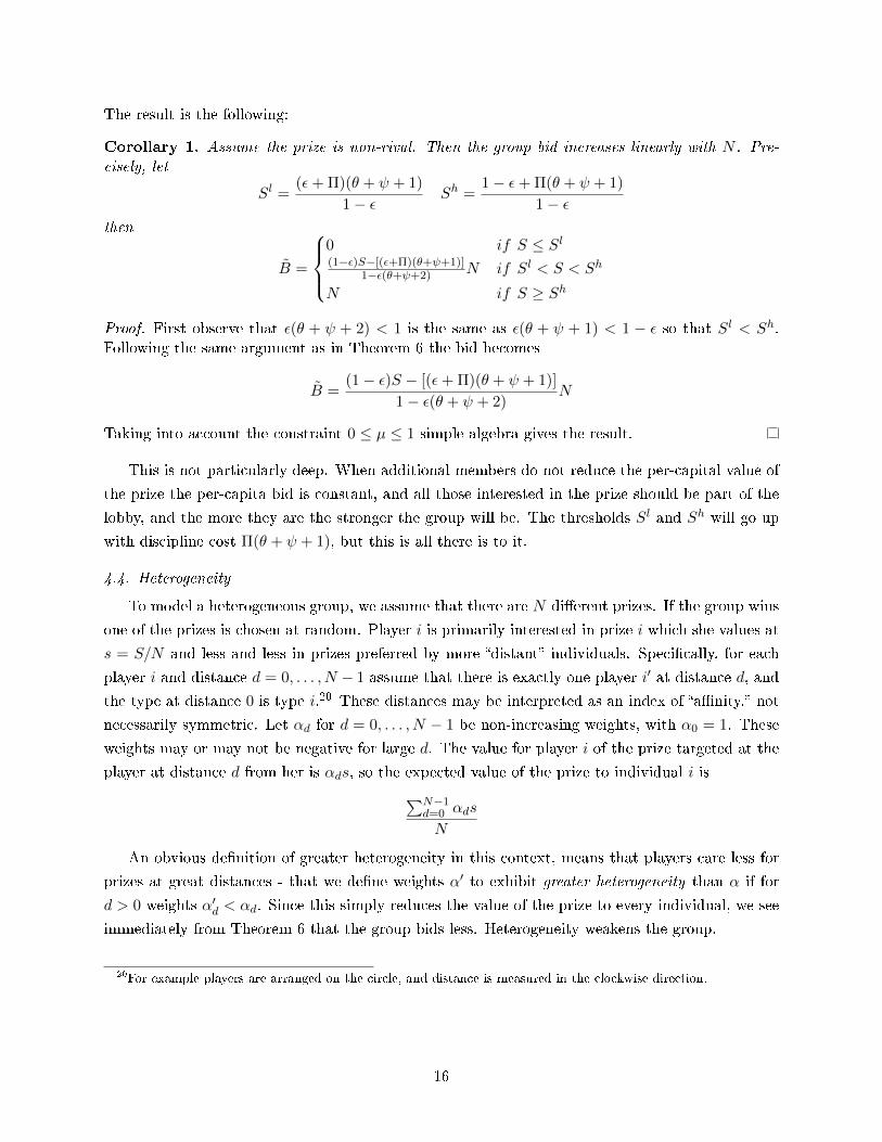
The result is the following:

Corollary 1. Assume the prize is non-rival. Then the group bid increases linearly with N . Pre-cisely, let

Sl =(ε+ Π)(θ + ψ + 1)

1− εSh =

1− ε+ Π(θ + ψ + 1)

1− εthen

B =

0 if S ≤ Sl(1−ε)S−[(ε+Π)(θ+ψ+1)]

1−ε(θ+ψ+2) N if Sl < S < Sh

N if S ≥ Sh

Proof. First observe that ε(θ + ψ + 2) < 1 is the same as ε(θ + ψ + 1) < 1 − ε so that Sl < Sh.Following the same argument as in Theorem 6 the bid becomes

B =(1− ε)S − [(ε+ Π)(θ + ψ + 1)]

1− ε(θ + ψ + 2)N

Taking into account the constraint 0 ≤ µ ≤ 1 simple algebra gives the result.

This is not particularly deep. When additional members do not reduce the per-capital value of

the prize the per-capita bid is constant, and all those interested in the prize should be part of the

lobby, and the more they are the stronger the group will be. The thresholds Sl and Sh will go up

with discipline cost Π(θ + ψ + 1), but this is all there is to it.

4.4. Heterogeneity

To model a heterogeneous group, we assume that there are N di�erent prizes. If the group wins

one of the prizes is chosen at random. Player i is primarily interested in prize i which she values at

s = S/N and less and less in prizes preferred by more �distant� individuals. Speci�cally, for each

player i and distance d = 0, . . . , N − 1 assume that there is exactly one player i′ at distance d, and

the type at distance 0 is type i.20 These distances may be interpreted as an index of �a�nity,� not

necessarily symmetric. Let αd for d = 0, . . . , N − 1 be non-increasing weights, with α0 = 1. These

weights may or may not be negative for large d. The value for player i of the prize targeted at the

player at distance d from her is αds, so the expected value of the prize to individual i is∑N−1d=0 αds

N

An obvious de�nition of greater heterogeneity in this context, means that players care less for

prizes at great distances - that we de�ne weights α′ to exhibit greater heterogeneity than α if for

d > 0 weights α′d < αd. Since this simply reduces the value of the prize to every individual, we see

immediately from Theorem 6 that the group bids less. Heterogeneity weakens the group.

20For example players are arranged on the circle, and distance is measured in the clockwise direction.

16

4.5. Voluntary Contributions With Prizes That Can Be Withdrawn

We now compare the predictions of the previous section with those of the alternative �usual�

voluntary public goods contribution model. Realized group e�ort level E is a noisy signal of intended

group e�ort µN . When a peer mechanism is implemented there is no useful information in this

signal since individual contributions are directly observed. However, if it is possible to withdraw

the prize based on E a voluntary contribution mechanism may be used to provide an incentive for

a positive level of contributions.

Suppose the group commits to a voluntary level of per capita contribution µ. It does so by send-

ing independent messages with probability µ indicating that individual e�ort should be provided.

Such a bid is feasible if it is in fact incentive compatible to follow those recommendations. If these

recommendations are followed the realized e�ort level E will follow a binomial with parameters µ

as success probability and N as number of trials. If the prize cannot be withdrawn then there is no

incentive to provide e�ort. Suppose instead that the bid includes a threshold µ with the agreement

that if e�ort level E falls below Nµ the prize will be withdrawn.

Observe �rst that a necessary condition for voluntary contribution is s ≥ 1. Otherwise even an

individual who will lose the prize for sure if he does not contribute will not do so. Consider �rst

the case µ = 1, where everyone is called to contribute. If the threshold µ = 1 then the prize will

be withdrawn if any single person fails to contribute regardless of N . Hence if s ≥ 1 voluntary

contribution by everyone is incentive compatible. However, this result is heavily dependent on

the fact that the aggregate statistic E is a perfect signal of individual behavior. In practice some

people will be unable to contribute because of other obligations, health problems, and so forth and

so on, and indeed the size of the group may not be known with perfect accuracy. A simple way to

model this in the current framework is to assume that there is an upper bound µ < 1 and that it is

infeasible to send signals with probability µ > µ. The remaining probability 1− µ may be thought

of as �the chance that the person is unable to contribute.� This leads to a radically di�erent result:

Theorem 7. For all s and 1 > µ > µ > 0 there exists an N such that N > N implies that anyincentive compatible µ < µ.

The key feature of this result is that the number N depends on s rather than S. In particular,

if the per capita size of the reward s is �xed, then if the group size is large enough there will be

no voluntary contribution. By contrast in the peer discipline case the threshold N is linear in S.21

If the per capita size of reward s is �xed and the group size is expanded, then the threshold N

increases in proportion. Think of this in terms of, for example, the farm lobby seeking a per farmer

subsidy of s. In the voluntary contributions model, a large country with many farmers would have

an ine�ective farm lobby, since N is very large. In the peer discipline case the size of the country

does not matter for the e�ectiveness of the farm lobby. As we observe that the farm lobby has

21With the upper bound on µ the maximum bid N changes because instead of B > N we must consider B > µNand the optimal group size becomes N = (1 − ε)S/[µ− ε(2µ− 1 − (1 − µ)(θ + ψ)) + κ] which is increasing in µ butmore important remains linear in S.

17

similar e�ectiveness in large countries such as the United States and smaller ones such as Japan,

there is some reason to believe that the absolute size of the group is not important. Moreover, in

the U.S. there are about 3 million farmers and 2 million farms. In particular, the public goods

problem that must be overcome by the group if there are to be voluntary contributions seems nearly

insurmountable.

Remark. One alternative explanation as to why the e�ectiveness of a group does not depend onthe absolute size for a �xed per capita prize is that contributions are voluntary but players arealtruistic. A standard model of altruism distinguishes between personal utility ui for player iand and uG =

∑j 6=i uj for other group members, and makes the hypothesis that the individual

maximizes a weighted sum ui+αNuG. In the voluntary contribution model this amounts to havingthe individual prize valued at (1 +αNN)s. There are two cases. If αNN remains bounded for largeN then the basic result goes through unchanged. However, if αNN grows without bound then theresult can be overturned. However it is implausible that αNN grows without bound. Consider theproblem of voluntary provision of taxes τi to provide a public good. Let τG =

∑j 6=i τj and assume

the value of the public good is v(τi+τG). The individual objective function is (1+αNN)v(τi+τG)−τi.The corresponding �rst order condition for voluntary contribution is v′(τi + τG) = 1/(1 +αNN), soin a large group voluntary contributions are so large that v′ is nearly zero, that is, the saturationpoint for the public good is reached. However, the condition for e�ciency is that v′(τi + τG) = 1so there are far too many contributions. Hence there should be no need in a large country like theUnited States to tax in order to provide (say) for defense spending - indeed, the problem shouldbe to discourage the ine�ciently high level of private contributions. This is the case even if weassume that individuals care only for people of a similar type - even if farmers care only for otherfarmers, the fact that there 3 million of them would probably be adequate to raise enough moneyto pay for the defense budget through voluntary contributions. The point is that if farmers arecontributing voluntarily to farm lobbying because they are altruistic towards other farmers, theyshould be very happy indeed to contribute voluntarily to the national defense. Of course publicgoods contributions are not carried out through voluntary contributions, but using punishment fornon-compliance.

Remark. Theorem 7 is a variation on the literature on the negligibility of agents, especially Mailathand Postlewaite [40], Levine and Pesendorfer [36] and Fudenberg, Levine and Pesendorer [23]. Thisliterature asks when a Stackelberg leader can punish a group of N followers based on an aggregatesignal to induce a desired behavior. The result - which is quite robust - is that this is not possibleif there is noise in the individual signal of behavior that is aggregated.

5. Competing Groups

Because the BDM mechanism is compatible with the second price auction, we can extend the

previous analysis to consider two groups that compete in a second price auction. We suppose that

the groups are identical except for their size. We are interested in which group will win the bidding,

and in the resulting e�ciency implications. We are also interested in endogenizing the size of the

prize - we consider how the di�erent groups and the seller might choose the size of the prize.

We shall work again in the low punishment cost case in which ε(θ + ψ + 2) ≤ 1 and

(θ + ψ + 1)ε(1 + Π)

1− ε< 1.

18

Let N1 < N2 be the group size, and consider �rst the case where the prize has a �xed value S, the

same for both groups. From Theorem 6 we immediately �nd

Corollary 2. When both groups value the prize equally

1. if N1 ≥ ˆN both groups bid zero; otherwise

1. if N1 ≥ N or N2 ≥ ˆN the small group wins

2. if N2 ≤ N the large group wins

3. if N1 < N < N2 ≤ ˆN there are cases where either group may win

Basically this shows that it is advantageous to be small but not too small - that it is advantageous

to be close to N .

Suppose now that the two groups value the prize di�erently, bearing in mind that N = N(S).

If one group values the prize more, that increases the chances of winning, but a group closer to

N may never-the-less win despite the fact it values the prize less. We can identify three di�erent

kinds of e�ciency losses as a result of this bidding procedure.

1. If the prize is valued di�erentially by the two groups the prize can to the wrong group.

2. If the winning group pays a positive price, then there is a social cost to the punishment that

takes place on the equilibrium path.

3. If the winning group pays a positive price the e�ort provided may be socially costly. It seems

usual in the literature about lobbying - for example Hillman and Samet [27] or Ehrlick and Lui

[20] - that this e�ort is socially costly. Whether this is true in general depends on the value of the

e�ort to the group versus the recipient of the e�ort: if the e�ort is �getting out the vote� it is a

social loss; if the e�ort is �shining the shoes of the politician� and he likes his shoes shined it may

be partially a transfer payment (hence no e�ciency loss) depending on the value to him of having

his shoes shined, versus the value of the e�ort to the provider.

Related to the �nal point - there is an important issue with laws designed to prevent bribery.

They may simply result in ine�cient bribes. That is, cash transfers are relatively e�cient, while

�shoe shining� isn't. If the bribe is simply that I work at my highest valued occupation and give

you some of the proceeds there isn't an e�ciency loss. If the bribe requires me to work at a lower

valued occupation (�shoe shining� when I'm a heart surgeon) then there is an e�ciency loss from

my working in a less valuable occupation.

5.1. Agenda Setting: Endogenous Prizes

We continue to study two groups of size N1 < N2 competing for a prize in a second price auction.

Now however, as in the political area, we will assume that the prize is a transfer payment between

the groups and analyze agenda setting. Speci�cally we will consider respectively the agenda being

set by the small group, by the large group, and by the seller - the politician. The agenda setter will

determine two things: which group j will pay for the transfer, and how large the transfer - the prize

S - is. Given the agenda the politician auctions the prize in a second price auction, collects the

winning bid, and commands the designated group j to pay the prize (more precisely min{S,Nj}) to

19

the winner. Note that the winner may be group j itself; in this case they are paying the politician

to avoid being taxed even more.

Obviously if it is one of the groups setting the agenda they will designate the other to pay -

that is, they will propose the legislator a transfer from the other group to their advantage - and

strategically choose the size of the prize so that they win the auction. The maximum group j can

pay is Nj (when they provide full e�ort), so the largest prize that group 2 can choose is N1 and

the largest prize that group 1 can choose is N2. The politician on the other hand can choose which

group will make the transfer as well as the size of the prize.

We also assume that for a given utility all groups lexicographically prefer a smaller prize to a

larger one. In case of a tie in the bidding, we impose the continuity requirement that the group

that would win when the prize was slightly higher wins the tie. The following may be seen as the

second main result of the paper.

Theorem 8. We consider again the low punishment cost case. A transfer takes place only if thesmall group sets the agenda, in which case it sets the prize S to

SL2 ≡ (θ + ψ + 1)ε+ Π

1− εN2,

bids a positive amount and pays zero; the large group pays min{SL2 , N2} to the small group. If thelarge group sets the agenda, it sets the prize equal to zero.

The winning group pays a positive amount only if the politician sets the agenda, in which caseshe chooses the large group to pay for the prize, which she sets equal to

S ≡N1[1− ε(θ + ψ + 2)] +N2

[(ε+ Π)(θ + ψ + 1)

]1− ε

Both groups bid N1 and the large group wins the bidding, so there is no transfer between the groupsbut simply a payment by the large group of N1 to the politician.

Proof. If the small group sets the agenda it will call the highest prize for which the large group

bids zero, that is the S for which N2 =ˆN , that is SL2 . It will not set a higher prize because

the transfer to their advantage goes up more slowly (slope 1) than the other group's bid (slope(1 − ε)/[1 − ε(θ + ψ + 2)]). The large group has nothing to win in this game because to win theywould have to bid at least N1 to the politician (from Corollary 2) to get at most N1 from the smallgroup. The politician on the other hand maximizes the lower bid (which is what she gets), whoseupper bound is N1. This is achieved by having both groups bid N1, which occurs when the largerone bids that much. From the equation B(N2) = N1 we then get S.

It is useful to have an idea of how much bribes are actually paid. Bribes include campaign

expenditure and also things like employment of o�cials after they leave o�ce. Data on presidential

campaigns from Floating Path [21] shows that this is quite small, less than 0.1% of GDP. This

suggests that the agenda setting ability lies with the outside groups and not with the politicians:

that politicians cannot simply threaten transfer payments in order to collect bribes. It also suggests

that, in accordance with our result, in general it is small groups who obtain transfers from larger

groups, at low �political� cost.

20

5.2. Di�erential Productivity

A group of size N may be more productive, so each unit of e�ort translates into A units of bid.

If the prize S is in dollar units, then the prize in e�ciency units is S/A and the dollar bid is derived

by multiplying the e�ort bid by A so that in the low punishment cost case

AB ≡ A(1− ε)(S/A)−N

[(ε+ Π)(θ + ψ + 1)

]1− ε(θ + ψ + 2)

=(1− ε)S −AN

[(ε+ Π)(θ + ψ + 1)

]1− ε(θ + ψ + 2)

which is identical to the dollar bid for a group of size AN and unitary productivity. Note that this

determines also N andˆN , and that when ε(θ + ψ + 2) ≥ 1 the groups bid AN . Hence a group of

sizes N and productivity A chooses the same bid as a group of size AN .

This says that a group that is twice as productive, but has half as many members is exactly as

e�ective as a group twice as big but half as productive. It is the total resources controlled by the

group that matters (in e�ect). You might think that a group twice as productive but half the size

would be more e�ective. But it is not: the problem is that while it has half as many members, so

that halves the �xed cost of peer discipline, the per-capita discipline costs it twice as much since

the cost in e�ort is the same but each unit of e�ort has a double opportunity cost in dollars. Or to

say it di�erently: the productive guys do not have to work as hard to produce a given bid, but it

is pretty expensive for them to waste their time monitoring each other.

As an example, think about in�uence within an academic department. There are those who are

very productive and those who are not. The productive ones can be more in�uential per unit time,

but don't waste their time organizing their productive peers to lobby with the administration. So

the department is run by the unproductive ones.

6. Conclusion

The broad issue we have addressed is the relation between size, cohesion and the strength of

groups. Since the pioneering work of Olson [45] the presumption has been that smaller, more ho-

mogeneous groups may perform better owing to the increased easiness of enforcing group discipline.

This idea is of course challenged by the observation that large groups may be harder to coordinate

but have nonetheless more weight in the political arena.

To address this we have developed a model of group behavior with explicit account of individual

incentives inside the group. The model seems more descriptively realistic than the voluntary con-

tribution model, and makes more appropriate predictions with respect to large groups. To analyze

the strength of the group we look at the amount of e�ort the group can enforce on its members in

a second price auction. We have considered two di�erent contexts. The �rst is one where the prize

comes from outside a single group or a pair of competing groups, typically a politician; the second

is a situation where two groups compete for a prize which is a transfer from a group to the other -

at a cost to be paid to the politician.

In the �rst case we have found that Olson's original idea that small groups are stronger needs

to be re�ned. It is true that larger groups bid more the larger the prize, but for a given prize there

21

is an �optimal�, highest-bidding group size, which outperforms both smaller and larger groups.

Moreover, the analysis reveals that when the same prize is valued di�erently by di�erent competing

groups ine�ciencies in allocation of the prize are likely to emerge, and this has subtle implications

for anti-corruption policy.

In the case of two groups contending a transfer granted by a politician from one group to

another - where the politician awards the group which grants her a higher payo� - we �nd instead

that indeed smaller groups have an advantage, and usually secure themselves the transfer from the

larger group, at low �political� cost, by taking the initiative and strategically choosing the size of

the transfer.

We have not pursued all aspects of the model, focusing largely on the issue of group size. The

model has implications as well for the role of information in internal discipline, issues which we

hope to examine in greater detail in future work. Also, we have treated the costs of punishment

as exogenous. To the extent that they can take of form of transfer payments as in La�ont [33] the

cost on the equilibrium path can be reduced. If the cost to the auditor can be made equal to zero

(θ = 0) and the cost to the auditee is a transfer payment to the rest of the group (ψ = CG/P = −1)

then the cost to the group of peer discipline is zero. This is analogous to the usual folk theorem

in repeated games with private information, as in Fudenberg Levine and Maskin [22] where the

discount factor approaching one makes it possible for future rewards and punishments to e�ectively

act as transfer payments.

The peer discipline setting allows the consideration of di�erent types of monitoring schemes.

Trial by press or peer pressure to conform are simple informal schemes. Often more formal judicial

schemes are used - for example �ring an employee may require formal hearings. Formal schemes

systematically consider evidence. On the one hand, this means that the signals of malfeasance

are more accurate. On the other hand, a higher level of evidence is generally required, so while

punishment of the innocent is less likely, punishment of the guilty is less likely as well. Using an

underlying signal structure with thresholds such as that in Fudenberg and Levine [24] we can see

how di�erent formal and informal schemes will impact on collusion constraints. Another common

method of reducing incentives for collusion is through rotation. Military and police organizations

often rotate o�cials from one position and location to another and politicians have term limits.

This can have the e�ect of degrading the quality of service provided while increasing the quality of

audits.

Notice that the parameters of signal quality and the chances of being caught depend also on

social characteristics. Groups that have been in existence for a long time and are suspicious of

outsiders will be better able to provide incentives - and also harder to prevent from engaging in

bad behavior - than shorter-lived more open groups. Through this channel, culture may have an

impact on group incentives; and conversely as people specialize in ways most suited to the group

they are in. Policy can also play a role - for example by rules against nepotism. There are many

cross-cultural experiments on trust and other simple games - we would like also to see what impact

culture has on our games played between groups.

22

Ultimately we may anticipate a better theory of mechanism design - a theory of mechanisms

that are robust to group collusion. Colluding groups and their internal incentives are important

for two reasons. For some groups - productive groups such as business �rms, or regulatory agencies

- e�ciency will demand strong incentives. For other groups - rent seekers and lobbying groups -

e�ciency will demand weak incentives. While a formal theory of peer discipline is a start on such

a theory, we need also to understand how groups coordinate or may fail to coordinate, and when

and how groups are formed and membership determined.

Appendix: Proofs not included in text

Theorem. [3 in text] The non static-Nash enforceable initial action aR is incentive compatible forsome implementation if and only if |θ| < [πp − π]. In this case to maximize the average expectedutility of the group it is necessary and su�cient that the incentive constraints hold with equality foreach positive probability public history. The average expected equilibrium utility level per person is

uR −[πR0 +

|θ|[πp − π]− |θ|

π

](θ + ψ + 1)GR.

Proof. By Theorem 2 the stated utility level is attained by a two-stage implementation. Hence itsu�ces to show that no incentive compatible implementation can attain a higher utility level.

The the objective function is

u(ai, aR)− (1/N)E0

∞∑t=1

N∑i=1

(θ + ψ + 1)P it

where E0 is expectation conditional on information at beginning of round 0. De�ning P t =(1/N)E0

∑Ni=1 P

it we can further write this as

u(ai, aR)− E0

∞∑t=1

(θ + ψ + 1)P t.

Fix any equilibrium and consider now the decision by auditor i to punish j on B and not punishon G in round t. Under our assumption the only consequence of this decision is the expected costof punishment in this round EtC

it and the expected punishment conditional on getting a bad signal

in the subsequent round EtPj(i)t+1 where j(i) is the unique person who audits i in period t + 1 -

note that this is a random variable. The decision has no consequence for future decisions as anauditor and no e�ect on the distribution of the signals accruing to the current auditor. On theequilibrium path utility associated with being audited in period t conditional on the signal zjt is

Et[Cit |z

jt ] + Et[P

j(i)t+1 |z

jt ]. Consider now those audit rounds for which t > 1. Conditional on the

bad signal, deviating to not punishing results in punishment increment ([πp − π]/π)Et[Pj(i)t+1 |B] =

([πp − π]/π)EtPj(i)t+1 , equality following from the fact that on the equilibrium path your chance of

being punished next period is by assumption independent of the signal your auditee has this period.

Cost saving on the other hand is Et[θPit |B]; so that the incentive constraint is ([πp−π]/π)Et[P

j(i)t+1 ] ≥

Et[θPit |B]. Since Et(P

it |B) = Et(P

it )/π, we may write this as [πp − π]EtP

j(i)t+1 ≥ θEtP it , . A similar

calculation conditioning on the good signal yields [πp − π]EtPj(i)t+1 ≥ −θEtP it . Combining the two

gives [πp − π]EtPj(i)t+1 ≥ |θ|EtP it .

23

Adding up the constraints across individuals and taking time zero expectations, we discoverthat [πp − π]P t+1 ≥ |θ|P t. Examining the objective function, we see that if this holds with strictinequality the objective function is increased by reducing P t+1 until it holds with equality. Thismay not be feasible, depending on the matching and so forth, but the constraints holding withexact equality provides an upper bound on the objective function given by solving the di�erenceequation [πp − π]P t+1 = |θ|P t for t > 1. In the �rst audit round, punishment is P 1 = πR0 G

R.Also, for t = 1 it is E1(P i1|B) = E1(P i1)/πR0 since the probability of the bad signal in the �rst

audit round is πR0 , so the incentive constraint ([πp − π]/π)E1[Pj(i)2 |B] ≥ E1[θP i1|B] reads ([πp −

π]/π)E1Pj(i)2 ≥ E1θP

i1/π

R0 ; combining this with the constraints for t > 1 and taking expectations

yields P 2 = (π/πR0 )(|θ|/[πp−π])P 1, equality as before being a lower bound. Substituting these plusthe solution to the di�erence equation into the objective function then gives the desired bound.Note that the condition |θ| < [πp − π] is necessary and su�cient for the sum in the objectivefunction to converge.

Theorem. [4 in text] If

Π ≤ (1− µ)(1− 2ε)

ε

group utility maximization implies β00 = β10 = β11 = 0, β01 = 1. Otherwise β10 = β11 = 0 andβ00 = β01 = 1.

Per capita group utility being equal to

s− µ− (θ + ψ + 1) min{(1− µ)ε+ Π

1− ε, (1− µ) + Π}

Proof. The conditions for enforceability of [01] are

u(ai, [01])− u([01], [01]) ≤ [π0(ai, [01])− π0([01], [01])]P1, ai = [00], [11], [10]

First u([00], [01]) − u([01], [01]) = µ > 0 implies P1 > 0. The conditions for [00] and [11] can bewritten respectively as

1/P1 ≤ (1− ε)(β01 − β11) + ε(β00 − β10)

1/P1 ≥ ε(β01 − β11) + (1− ε)(β00 − β10)

and they are the only relevant ones because as is easily checked by summing them one gets the con-dition for [10]. Since u([11], [01])− u([01], [01]) = −(1−µ) < 0 we then have G(aR) = G([00], [01]).The objective is to minimize

[π0([01], [01]) + Π](θ + ψ + 1)G([00], [01])

subject to enforceability.The two above enforceability inequalities imply - together with P1 > 0 - that [01] is enforceable

i�

β01 − β11 ≥ β00 − β10

(1− ε)(β01 − β11) + ε(β00 − β10) > 0

Observe that they imply β01 − β11 > 0. Incidentally: the set of vectors de�ned by the conditions

24

β10 = β11 = 0, 1 = β01 ≥ β00 satisfy the conditions. Now

G([00], [01]) =u([00], [01])− u([01], [01])

π0([00], [01])− π0([01], [01])=

1

(1− ε)(β01 − β11) + ε(β00 − β10)

π0([01], [01]) = µ(1− ε)β11 + (1− µ)εβ01 + µεβ10 + (1− µ)(1− ε)β00

Clearly both π0([01], [01]) and G([00], [01]) go down with β11 and β10 hence β11 = β10 = 0. Firstobserve that if µ = 1 then π0 = 0 so the minimum of the objective function is achieved by settingβ00 = β01 = 1. Suppose now that µ < 1.

Dividing by the constant (1− µ)(θ+ψ+ 1) the objective function is maximized by minimizingthe function

εβ01 + (1− ε)β00 + Π(1−µ)

(1− ε)β01 + εβ00

The derivative with respect to β01 is

−(1− 2ε)β00 − (1− ε) Π(1−µ)

[(1− ε)β01 + εβ00]2,

hence the optimal β01 = 1. Then the derivative with respect to β00 is

(1− 2ε)− εΠ(1−µ)

[(1− ε) + εβ00]2.

From this it follows that if 1− 2ε ≥ εΠ/(1− µ) then β00 = 0, and β00 = 1 otherwise. Plugging thisinto the objective function we obtain that: if

Π ≤ (1− µ)(1− 2ε)

ε

we have π0([01], [01]) = (1− µ)ε and GR = 1/(1− ε), hence per-capita utility is given by

s− µ− [(1− µ)ε+ Π](θ + ψ + 1)1

1− ε;

otherwise we have π0([01], [01]) = 1− µ and G([00], [01]) = 1, thus per-capita utility is

s− µ− [(1− µ) + Π](θ + ψ + 1)

Now it is easily checked that the condition Π ≤ (1− µ)(1− 2ε)/ε is equivalent to

(1− µ)ε+ Π

1− ε≤ (1− µ) + Π

and this yields the desired result.

Theorem. [6 in text] The bid function is single peaked as a function of N . De�ne

N =S

1 + (θ + ψ + 1)ΠˆN =

S

(θ + ψ + 1) ε+Π1−ε

25

For N ≤ N the bid is N . If ε(θ + ψ + 2) ≤ 1 and

(θ + ψ + 1)ε(1 + Π)

1− ε< 1

thenˆN > N and for N ≤ N ≤ ˆ

N the bid is given by the following function, decreasing in N :

B ≡(1− ε)S −N

[(ε+ Π)(θ + ψ + 1)

]1− ε(θ + ψ + 2)

In all other cases the group does not bid.

Proof. It is easily seen that the group payo� from a bid of µ can be written as

Payoff(µ) = S −Nµ−N(θ + ψ + 1)×

{(1−µ)ε+Π

1−ε µ ≤ 1−(2+Π)ε1−2ε

1− µ+ Π otherwise

whose derivative with respect to µ is{N( (θ+ψ+1)ε

1−ε − 1)

µ ≤ 1−(2+Π)ε1−2ε

N(θ + ψ) otherwise

Case 1 (high punishment cost): (θ+ψ+2)ε > 1. In this case the payo� is increasing in µ throughoutits interval, so the group bids µ = 1 if Payoff(1) ≥ 0 and nothing otherwise. And the non-negativitycondition amounts to N ≤ N .

Case 2 (low punishment cost): (θ + ψ + 2)ε ≤ 1. In this case the payo� is U-shaped. IfPayoff(1) ≥ Payoff(0) again the group will bid 1 if Payoff(1) ≥ 0 and zero otherwise; the non-negativity condition is the same as before, N ≤ N , while the inequality is satis�ed i�

(θ + ψ + 1)ε(1 + Π)

1− ε≥ 1

If this last inequality is reversed, then for N ≤ N we still have Payoff(1) ≥ 0 so the group stillbids 1. For N > N on the other hand Payoff(1) < 0 so the group's bid is given by the µ at whichthe decreasing part of the payo� crosses zero, which is easily computed as the function B = B(N)

given in the statement, which decreases and reaches zero at N =ˆN > N , the latter inequality

following from (θ + ψ + 1)ε(1 + Π) < (1− ε). Theorem now follows.

Theorem. [7 in text] For all s and 1 > µ > µ > 0 there exists an N such that N > N implies thatany incentive compatible µ < µ.

Proof. Let ΦN (x) be the cdf of the standardized binomial, that is, the probability that a binomialx with success probability µ and N trials has (x − Ex)/

√var(x) ≤ x. With E representing total

e�ort, the prize is awarded if E ≥ Nµ. Passing to standardized variables one �nds that if you geta message and you contribute you get s with probability 1−ΦN ((µ− µ)

√N/√µ(1− µ)), and pay

an e�ort cost of 1. On the other hand if you get a message and you do not contribute you get swith probability

1− ΦN−1([N

N − 1µ− µ]

√N − 1√µ(1− µ)

)

26

Hence the gain to not contributing is

GN = s[ΦN ((µ− µ)

√N√

µ(1− µ))− ΦN−1([

N

N − 1µ− µ]

√N − 1√µ(1− µ)

)]

+ 1.

Suppose µ ≤ µ ≤ µ. It is easy to show that when |µ − µ|√N is large enough - say N > N1 -

the two probabilities are either both close to one (if µ < µ) or both close to zero (if µ > µ), usingthe Chebyshev inequality. Thus in that case it will be optimal not to contribute. If µ 6∈ [µ, µ] this

ends the proof. Suppose not, and that for some χ it is |µ − µ|√N ≤ χ (so that µ → µ). Now we

will use the Central Limit Theorem to argue that since both ΦN−1 and ΦN are close to a standardnormal Φ they are close to each other. Because µ ≤ µ ≤ µ and the bound χ the Central LimitTheorem applies uniformly. The di�erence

[N

N − 1µ− µ]

√N − 1− (µ− µ)

√N =

1√N − 1

µ− (µ− µ)1√

N +√N − 1

is uniformly close to zero. Since Φ is continuous it then follows that there exists an N2 such thatfor N > N2 we again have GN > 0.

Theorem. [8 in text] A transfer takes place only if the small group sets the agenda, in which caseit sets the prize S to

SL2 ≡ε(θ + ψ + 1) + κ

1− εN2,

bids a positive amount and pays zero; the large group pays min{SL2 , N2} to the small group. If thelarge group sets the agenda, it sets the prize equal to zero.

The winning group pays a positive amount only if the politician sets the agenda, in which caseshe chooses the large group to pay for the prize, which she sets equal to

S ≡N1[1− ε(θ + ψ + 2)] +N2

[ε(θ + ψ + 1) + κ

]1− ε

Both groups bid N1 and the large group wins the bidding, so there is no transfer between the groupsbut simply a payment by the large group of N1 to the politician.

Proof. Recall that

Bj ≡(1− ε)S −Nj

[ε(θ + ψ + 1) + κ

]1− ε(θ + ψ + 2)

.

Observe that since we always assume θ + φ+ 1 > 0 we have

1− ε1− ε(θ + ψ + 2)

> 1

so that the bid increases faster than the prize. The following is the prize size below which group jbids zero:

SLj ≡ε(θ + ψ + 1) + κ

1− εNj

Note that SLj > Nj for κ large enough. The following is the prize size for which group j posts thehighest bid:

SHj ≡1− ε+ κ

1− εNj

27

Observe that ε(θ + ψ + 2) < 1 is the same as ε(θ + ψ + 1) < 1 − ε, so that SLj < SHj . A group of

size Nj bids zero for S ≤ SLj then the bid increases linearly, it reaches Nj for S = SHj and remainsconstant for larger S.

Below S < SL1 both groups bid zero. Between SL1 and SL2 group 1 bids min{B1, N1}, wins theauction and pays zero, getting a surplus of S. If SH1 > SL2 then between SL2 and SH1 group 1 bidsB1, wins the auction, pays the bid B2, getting a surplus of S − B2 which decreases in S. AboveSH1 group 1 bids N1, wins the auction and pays B2 until S equals

S =N1[1− ε(θ + ψ + 2)] +N2

[ε(θ + ψ + 1) + κ

]1− ε

.

Above S group 2 wins and pays N1. If SH1 < SL2 the only change is that the range over which the

small group pays zero is larger. The winning group is unchanged.Now consider who sets the agenda. Because the bid increases faster than the prize, when the

small group has the agenda, they should choose a prize of SL2 and pay zero (regardless of the relativesizes of SH1 and SL2 ). The large group will have to pay a transfer of min{SL2 , N2} to the smallerone.

Suppose the large group chooses S. It can only win by choosing S > S in which case it paysN1, however the size of the prize cannot be larger than N1, so as it can never get any surplus itprefers the smallest prize S = 0. No transfer will take place.

Suppose lastly that the politician chooses S. She will do so to maximize the lower bid, which iswhat she collects. The bids are increasing in the size of the prize, but limited by the ability of thesmall group to pay no more than N1. The large group is willing to pay N1 only above S, while thesmall group is willing to pay N1 above SH1 < S. To get N1 in a second price auction both groupshave to be willing to pay N1, which means that we must have S ≥ S. Notice that SH1 > N1 so Sis as well. Hence it is only feasible to charge S if the prize is paid for by the large group. Above Sthe lower bid remains constant at N1 (and the large group wins by bidding strictly more), so sinceboth groups prefer lower prize values the politician will set S = S and get N1 from the large group- which by assumption wins the tie and pays N1 to the politician to avoid paying S > N1 to thesmall group.

References

[1] Abreu, D., D. Pearce, E. Stacchetti (1986): "Optimal cartel equilibria with imperfect moni-toring," Journal of Economic Theory

[2] Acemoglu, Daron (2001): "Ine�cient redistribution", American Political Science Review Vol.95, pp. 649-661.

[3] Ades, A. and R. DiTella (2002): "The new economics of corruption: a survey and some newresults," Political Studies.

[4] Austen-Smith, David and J. R. Wright (1992): "Competitive lobbying for a legislator's vote,"Social Choice and Welfare.

[5] Banks, Je�rey S. and Barry R. Weingast (1992): "The political control of bureaucracies underasymmetric information," American Journal of Political Science.

[6] Becker, G. S. (1983): �A theory of competition among pressure groups for political in�uence,�Quarterly Journal of Economics 98: 371-400.

[7] Becker, Gary S. (1985): "Public policies, pressure groups, and dead weight costs", Journal ofpublic economics, 1985 - Elsevier

28

[8] Becker, Gary S. and Casey B. Mulligan (1998): "Deadweight costs and the size of government,"NBER.

[9] Becker, Gilbert (1986): "The Public Interest Hypothesis Revisited: A New Test of Peltzman'sTheory of Regulation", Public Choice Vol. 49, pp. 223-234.

[10] Boadway, R. and M. Keen (2000): "Redistribution," Handbook of income Distribution.

[11] Border, Kim C. and Joel Sobel (1987): "Samurai Accountant: A Theory of Auditing andPlunder", The Review of Economic Studies Vol. 54, pp. 525-540

[12] Cipolla, Carlo (1965): Guns, Sails, and Empires: Technological Innovation and the EarlyPhases of European Expansion, 1400- 1700.

[13] Dal Bo, P. (2005): �Cooperation under the shadow of the future: experimental evidence fromin�nitely repeated games,� American Economic Review.

[14] Damania, R., P. G. Frederiksson and M. Mani (2004): "The persistence of corruption andregulatory compliance failures: Theory and evidence," Public Choice.

[15] Diamond, Jared (1998): Guns, Germs, and Steel: The Fates of Human Societies.

[16] Di Porto, Edoardo, Nicola Persico and Nicolas Sahuguet (2013): "Decentralized Deterrence,with an Application to Labor Tax Auditing", American Economic Journal: Microeconomics Vol.5, pp. 35-62

[17] Dixit, Avinash (2004): Lawlessness and Economics, Princeton University Press

[18] Dixit, Avinash, Gene M. Grossman and Elhanan Helpman (1997): "Common Agency and Co-ordination: General Theory and Application to Government Policy Making", Journal of PoliticalEconomy Vol. 105, pp. 752-769

[19] Benoit, Jean-Pierre and Krishna, Vijay (1987): �Nash equilibria of �nitely repeated games,�International Journal of Game Theory 16: 197-204.

[20] Ehrlick, I. and F. Lui (2000): "Bureaucratic corruption and endogenous economic growth,"Journal of Political Economy.

[21] www.floatingpath.com/2012/03/05/campaign-spending-percentage-gdp/

[22] Fudenberg, Drew, David K. Levine and Eric Maskin (1994): �The folk theorem with imperfectpublic information,� Econometrica.

[23] Fudenberg, D., D. Levine and W. Pesendorfer (1998): �When are nonanonymous playersnegligible?� Journal of Economic Theory.

[24] Fudenberg, Drew and David Levine (2009): �Repeated Games with Frequent Signals,� Quar-terly Journal of Economics, 124: 149-195.

[25] Fudenberg, Drew and Eric Maskin (1986): �The folk theorem in repeated games with dis-counting or with incomplete information,� Econometrica.

[26] Green, Jerry and Jean-Jacques La�ont (1979): "On Coalition Incentive Compatibility", TheReview of Economic Studies Vol. 46, pp. 243-254

[27] Hillman, A. L. and D. Samet (1987): "Dissipation of contestable rents by small numbers ofcontenders," Public Choice.

[28] Jehiel, Philippe [2005]: �Analogy-based Expectation Equilibrium�, Journal of Economic The-ory 123: 81-104.

[29] Kandori, Michihiro (1992): �Social norms and community enforcement,� The Review of Eco-nomic Studies.

[30] Krishna, V. and J. Morgan (1997): "An analysis of the war of attrition and the all-payauction," Journal of Economic Theory.

29

[31] Kroszner, R. S. and T. Stratmann (1998): "Interest-group competition and the organizationof congress: theory and evidence from �nancial services' political action committees,"AmericanEconomic Review.

[32] La�ont, Jean-Jacques (1999): "Political economy, information and incentives," European Eco-nomic Review.

[33] La�ont, Jean-Jacques (2000): Incentives and political economy, Oxford University Press.

[34] La�ont, Jean-Jacques and Jean Tirole (1991): "The politics of government decision-making:A theory of regulatory capture," The Quarterly Journal of Economics.

[35] Levine, David K. and Salvatore Modica (2012) �Con�ict and the Evolution of Societies�, mimeo

[36] Levine, D. K. and W. Pesendorfer [1995]: �When Are Agents Negligible?� American EconomicReview, 85: 1160-1170

[37] Levine, David and Wolfgang Pesendorfer (2007): �The Evolution of Cooperation ThroughImitation,� Games and Economic Behavior.

[38] Li, John Shuhe (2003): �The Bene�ts and Costs of Relation-based Governance: an Explanationof the East Asian Miracle and Crisis�, Review of International Economics 11: 651-673

[39] Lohmann, Susanne (1998): "An Informational Rationale for the Power of Special Interests",American Political Science Review Vol. 92, pp. 809-28

[40] Mailath, George J. and Andrew Postlewaite (1990): �Asymmetric Information BargainingProblems with Many Agents�, Review of Economic Studies 57: 351-367

[41] McNeil, William (1963): The Rise of the West, University of Chicago Press.

[42] Mitra, D. (1999): "Endogenous lobby formation and endogenous protection: a long-run modelof trade policy determination," American Economic Review.

[43] Nitzan, Shmuel and Ueda, Kaoru (2011): �Prize sharing in collective contests,� EuropeanEconomic Review 55, pp. 678-687

[44] Nti, K. O. (1999): "Rent-seeking with asymmetric valuations," Public Choice 98, pp. 415-430.

[45] Olson, Mancur (1965): The Logic of Collective Action: Public Goods and the Theory ofGroups.

[46] Olson, Mancur (1982): The Rise and Decline of Nations: Economic Growth, Stag�ation, andSocial Rigidities, Yale University Press.

[47] Ostrom, Elinor (1990): Governing the Commons: The Evolution of Institutions for CollectiveAction, Cambridge University Press.

[48] Ostrom, Elinor, James Walker and Roy Gardner (1992): �Covenants with and Without aSword: Self-Governance Is Possible�, The American Political Science Review (86), pp. 404-417

[49] Pecorino, Paul (2009): �Public goods, group size, and the degree of rivalry�, Public Choice138, pp. 161-169.

[50] Persson, T. and G. Tabellini (2002): "Political economics and public �nance," Handbook ofpublic economics.

[51] Potters, Jan and Randolph Sloof (1996): "Interest groups: A survey of empirical models thattry to assess their in�uence", European Journal of Political Economy Vol. 12, pp. 403-442

[52] Shapiro, Carl and Stiglitz, Joseph E. (1984): �Equilibrium Unemployment as a Worker Disci-pline Device�, American Economic Review 74, pp. 433-444

[53] Slinko, Irina, Evgeny Yakovlev, and Ekaterina Zhuravskaya (2005), �Laws for sale: evidencefrom Russia,� American Law and Economics Review 7.1: 284-318.

[54] Sugaya T. (2011): �Folk Theorem in Repeated Games with Private Monitoring,� PrincetonUniversity.

30

[55] Uhlaner, C. J. (1989): "Rational turnout: The neglected role of groups," American Journalof Political Science.

[56] Wittman, Donald (1989): "Why Democracies Produce E�cient Results", Journal of PoliticalEconomy Vol. 97, pp. 1395-1424

31