Pedestrian demand forecasting

Guideline

Pedestrian demand forecasting February 2021

Guideline, Transport and Main Roads, February 2021

Copyright

© The State of Queensland (Department of Transport and Main Roads) 2021.

Licence

This work is licensed by the State of Queensland (Department of Transport and Main Roads) under

a Creative Commons Attribution (CC BY) 4.0 International licence.

CC BY licence summary statement

In essence, you are free to copy, communicate and adapt this work, as long as you attribute the

work to the State of Queensland (Department of Transport and Main Roads). To view a copy of this

licence, visit: https://creativecommons.org/licenses/by/4.0/

Translating and interpreting assistance

The Queensland Government is committed to providing accessible services to

Queenslanders from all cultural and linguistic backgrounds. If you have difficulty

understanding this publication and need a translator, please call the Translating and

Interpreting Service (TIS National) on 13 14 50 and ask them to telephone the

Queensland Department of Transport and Main Roads on 13 74 68.

Disclaimer

While every care has been taken in preparing this publication, the State of Queensland accepts no

responsibility for decisions or actions taken as a result of any data, information, statement or

advice, expressed or implied, contained within. To the best of our knowledge, the content was

correct at the time of publishing.

Feedback

Please send your feedback regarding this document to: [email protected]

https://creativecommons.org/licenses/by/4.0/

mailto:[email protected]

Guideline, Transport and Main Roads, February 2021 i

Contents

1 Introduction ....................................................................................................................................1

1.1 Background ..................................................................................................................................... 1

1.2 Related documents ......................................................................................................................... 1

1.3 Purpose ........................................................................................................................................... 1

1.4 Intended audience .......................................................................................................................... 1

1.5 How to use this guidance ................................................................................................................ 2

1.6 Limitations ....................................................................................................................................... 2

2 Methods selection..........................................................................................................................3

2.1 Overview ......................................................................................................................................... 3

2.2 Methods .......................................................................................................................................... 3

2.3 Procedures in this guideline ............................................................................................................ 4

3 Data collection ...............................................................................................................................5

3.1 Background ..................................................................................................................................... 5

3.2 Counts ............................................................................................................................................. 6

3.2.1 Counting duration ...........................................................................................................6 3.2.2 Atypical conditions ..........................................................................................................7 3.2.3 Count options .................................................................................................................7

3.3 Count specification ....................................................................................................................... 10

3.4 User perceptions and behaviour changes .................................................................................... 11

4 Factoring ...................................................................................................................................... 12

4.1 Introduction ................................................................................................................................... 12

4.2 Obtain pre-construction counts ..................................................................................................... 12

4.3 Purpose split ................................................................................................................................. 12

4.4 Diversion rates .............................................................................................................................. 14

4.5 Calculation method ....................................................................................................................... 16

5 Comparison methods ................................................................................................................. 17

5.1 Background ................................................................................................................................... 17

5.2 Counts database ........................................................................................................................... 17

6 Direct demand models ............................................................................................................... 18

6.1 Background ................................................................................................................................... 18

6.2 Model ............................................................................................................................................ 19

6.3 Implementation ............................................................................................................................. 21

7 Worked example ......................................................................................................................... 22

7.1 Comparison method ..................................................................................................................... 22

7.2 Factoring ....................................................................................................................................... 23

7.3 Direct demand............................................................................................................................... 23

7.4 Summary ....................................................................................................................................... 24

8 Conclusion .................................................................................................................................. 24

Pedestrian demand forecasting

Guideline, Transport and Main Roads, February 2021 1

1 Introduction

1.1 Background

The Queensland Government is committed to ensuring Queenslanders of all ages and abilities can

walk safely and comfortably, when and where they choose (Queensland Walking Strategy 2019–

2029). To assist practitioners in determining the merits of providing pedestrian infrastructure, and the

scale of that infrastructure, methods are required to forecast pedestrian demand.

1.2 Related documents

This document should be used in conjunction with the documents described in Table 1.2 which

provide further detail on design considerations and supplementary information. Further detail of

documents referenced in this guideline is provided in the Transport and Main Roads Active transport

users guidelines references.

Table 1.2 – Related documents

Publisher Title

Austroads Guide to Traffic Management Part 3: Transport Study and Analysis Methods (2020)

Development of the Australasian Pedestrian Facility Selection Tool (2015) (AP-R472-15)

Australasian Pedestrian Facility Selection Tool [V2.1]: User Guide (2018) (AP-R592-18)

Forecasting Demand for Bicycle Facilities (2001) (AP-R194)

1.3 Purpose

The intent of this document is to provide guidance to practitioners to forecast demand for pedestrians

for new infrastructure such as:

• footpaths or shared paths, including 'missing links' in an existing path network

• unsignalised road crossings such as pedestrian refuges, zebra or wombat crossings or grade

separated infrastructure, and/or

• signalised road crossings, including mid-block pedestrian operated signals and pedestrian

crossings at signalised intersections.

This guidance does not consider pedestrian simulation modelling; that is, the modelling of crowd

dynamics for purposes such as typical and emergency egress from train stations or sports stadiums.

1.4 Intended audience

This guidance is intended for transport planners proposing or designing pedestrian infrastructure who

need to assess the likely pedestrian demand as part of assessing the viability of the infrastructure.

Examples where pedestrian demand forecasts may be useful include:

• assessment of appropriate infrastructure using existing tools such as the Australasian

Pedestrian Facility Selection Tool

• business case development (including cost-benefit analysis)

https://www.tmr.qld.gov.au/Travel-and-transport/Pedestrians-and-walking/Queensland-walking-strategy

https://www.tmr.qld.gov.au/Travel-and-transport/Pedestrians-and-walking/Queensland-walking-strategy

https://www.tmr.qld.gov.au/business-industry/Technical-standards-publications/Cycling-guidelines

https://www.tmr.qld.gov.au/business-industry/Technical-standards-publications/Cycling-guidelines

https://austroads.com.au/publications/traffic-management/agtm03

https://austroads.com.au/publications/traffic-management/agtm03

https://austroads.com.au/publications/active-travel/ap-r472-15

https://austroads.com.au/network-operations/active-travel/pedestrian-facility-selection-tool

https://austroads.com.au/publications/active-travel/ap-r194-01



• new project planning either for standalone pedestrian projects or in conjunction with larger

road or public transport projects, and/or

• development assessment where a new development (residential, office, commercial and so

on) is proposed and the road authority wishes to understand the likely pedestrian demand

effects, including possible developer contributions.

The user is assumed to have knowledge of transport planning but may have limited knowledge of

transport modelling methods.

The scope of this guidance is limited to infrastructure; non-infrastructure programs such as travel

behaviour change campaigns are excluded.

1.5 How to use this guidance

This guidance consists of a general overview of the methods available for pedestrian demand

forecasting (Section 2), issues associated with data collection (Section 3) and three detailed

procedures in sections 4, 5 and 6. Practitioners are advised to review the general advice in sections 2

and 3 before implementing the procedures in sections 4, 5 and 6 for their projects. These procedures

are described in ascending order of complexity; however, every effort has been made to make them

as simple and rapid for practitioners to implement as possible. Furthermore, the three methods have

been implemented in an online tool at https://pedtools.com.au/forecasts. In most cases, it is

anticipated that practitioners will use this guideline in conjunction with the online tool.

Because of the uncertainty associated with pedestrian demand forecasting, practitioners are advised

to use all three procedures for a project to obtain a range of forecasts. In combination with

professional judgment, this should then provide a plausible range of forecasts which can be used in

further developing project proposals.

1.6 Limitations

Forecasting is inherently uncertain, and this is particularly true for pedestrian demand forecasting

where:

• existing data on pedestrian activity is limited, and often of variable quality

• pedestrian activity, particularly in areas of predominantly recreational activity, is highly

sensitive to weather and seasonal factors, and/or

• there is a wide variety of sociodemographic, land use and transport network-related variables

which will affect pedestrian activity; not all of these are readily measurable.

The guidance in this technical document is indicative as the forecasts guide on the quantum of

demand but are not precise indicators. The practitioner should treat the central estimates as a guide

only and consider sensitivity testing demand within the stated prediction intervals or, where justified by

local conditions, beyond these intervals.

Data limitations currently preclude the methods in this guidance from incorporating anticipated land

use changes such as new residential and commercial development and new or expanded primary and

secondary schools. Moreover, the forecasts apply to an average day and cannot be used to forecast

demand during special events. Finally, the models are based on empirical data from projects

implemented in Queensland over the past 10 years. The contexts in which these projects have been

implemented vary, but many involve relatively modest pedestrian improvements in areas with modest

pedestrian network quality and patchy network extent. Improved network quality would likely escalate

https://pedtools.com.au/forecasts



pedestrian demands beyond those predicted by these procedures. The model may be unduly

conservative in scenarios that seek to extrapolate beyond the realms of the existing data.

2 Methods selection

2.1 Overview

The most appropriate pedestrian demand forecasting method will depend on:

• the scale of the project – larger, more expensive projects present greater risks of wasted

expenditure, should the project underperform and, in any case, would be expected to have

more resources available to fund more sophisticated demand forecasting methods that the

scale of expenditure warrants

• the availability of data – in some locations, there will be some pre-existing pedestrian data

available, perhaps collected as part of a larger transport study: in many cases, only very

limited data may be available

• timing and budget – sophisticated approaches require significant time and financial

resources, which may not be available or warranted, and/or

• the opportunities / complexity of the project – projects in larger corridors which offer a range

of outcomes may benefit more from further investigation of pedestrian demand to guide

decisions around providing dedicated pedestrian infrastructure or sharing with other path

users, including bicycle riders.

Note: Pedestrian demand forecasting methods are in their infancy and even sophisticated approaches may not

necessarily produce more robust estimates than simpler approaches.

2.2 Methods

There are six general classes of pedestrian demand forecasting methods:

1. comparison study – obtaining counts for existing, similar projects and using these counts for

the proposed location

2. sketch planning – relatively simple calculation based on land uses, assumed trip generation

and distribution and often implemented in a spreadsheet; the details of the sketch planning

method will vary, depending on the data available and nature of the site

3. direct demand models – regression equations linking land use and transport network

characteristics to pedestrian demand

4. spatial analysis – an extension of sketch planning, and possibly involving direct demand

models, implemented in geographic information system (GIS) mapping, so more detailed

analysis of route choices may be undertaken to align with traditional traffic network models

5. discrete choice – probabilistic models of mode choice and, possibly, destination and route

choice, that enable feedback between demand and infrastructure provision in a behaviourally

realistic manner; the discrete choice method requires specialist expertise and is likely

implemented as part of a network model, and

6. network model – simplified representation of a transport network, usually including discrete

choice models for mode and destination choice and equivalent to models widely used in



motorised transport planning (and usually based on extensive traffic survey data) which have

rarely been implemented for pedestrians.

Figure 2.2 compares pedestrian demand forecasting method complexity for the six methods

described. Further details about these forecasting methods are provided in Austroads Guide to Traffic

Management Part 3 Transport Studies and Analysis Methods.

Figure 2.2 – Pedestrian demand forecasting method complexity

Practically all pedestrian demand forecasting methods are simplified comparison studies or sketch

plans, with only larger projects progressing to more sophisticated spatial analysis. As the methods

become more complex, they have increasingly onerous data requirements. Existing data sources,

such as the Census of Population and Employment and household travel surveys, provide limited or

infrequent pedestrian data. In many cases, additional data will need to be collected as part of applying

these methods (Section 3).

2.3 Procedures in this guideline

This guideline draws on two of the forecasting methods described in Section 2.2 to provide detailed

guidance on the application of three forecasting procedures:

1. factoring: an approach using a pre-construction count and applying growth factors to this

count to estimate post-construction demand (this is analogous to a comparison study)

2. similar conditions: a database of pedestrian counts from locations across Queensland that

can be used to estimate demand for a project (that is, a comparison study), and/or

3. direct demand model: regression models linking land uses such as population, employment

and schools to pedestrian demand.

Implementation of these procedures is either trivial (in the case of factoring) or assistance is provided

to practitioners in the form of an online tool to enable rapid forecasting using these procedures. All

three methods should be used for a project and practitioners should use these three estimates to

determine the most likely demand. A summary of the procedures is provided in Figure 2.3 and each is

described further in subsequent sections of this guideline.



Figure 2.3 – Summary flowchart of procedures

3 Data collection

3.1 Background

The collection of high-quality pedestrian data supports the development of improved pedestrian

demand forecasting methods. This section considers two types of pedestrian data collection:

1. counts, and

2. perceptions of users of a facility or route ('user perceptions').

A third type of data collection could involve non-user perceptions; that is, understanding why people

choose not to use a particular facility or route. This type of data collection is likely to be difficult and

beyond the scope of most projects, given it will require surveys of a wider population. Not all data

collection activities will be warranted for all projects; some pragmatism is warranted, depending on the

scale and level of innovation of a project.



3.2 Counts

3.2.1 Counting duration

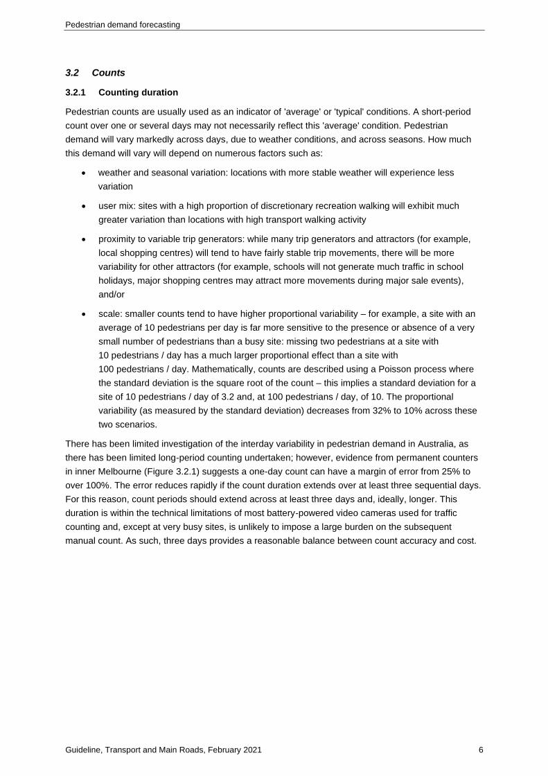
Pedestrian counts are usually used as an indicator of 'average' or 'typical' conditions. A short-period

count over one or several days may not necessarily reflect this 'average' condition. Pedestrian

demand will vary markedly across days, due to weather conditions, and across seasons. How much

this demand will vary will depend on numerous factors such as:

• weather and seasonal variation: locations with more stable weather will experience less

variation

• user mix: sites with a high proportion of discretionary recreation walking will exhibit much

greater variation than locations with high transport walking activity

• proximity to variable trip generators: while many trip generators and attractors (for example,

local shopping centres) will tend to have fairly stable trip movements, there will be more

variability for other attractors (for example, schools will not generate much traffic in school

holidays, major shopping centres may attract more movements during major sale events),

and/or

• scale: smaller counts tend to have higher proportional variability – for example, a site with an

average of 10 pedestrians per day is far more sensitive to the presence or absence of a very

small number of pedestrians than a busy site: missing two pedestrians at a site with

10 pedestrians / day has a much larger proportional effect than a site with

100 pedestrians / day. Mathematically, counts are described using a Poisson process where

the standard deviation is the square root of the count – this implies a standard deviation for a

site of 10 pedestrians / day of 3.2 and, at 100 pedestrians / day, of 10. The proportional

variability (as measured by the standard deviation) decreases from 32% to 10% across these

two scenarios.

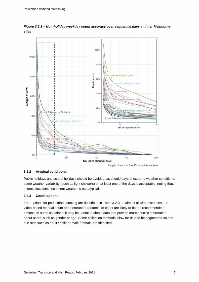
There has been limited investigation of the interday variability in pedestrian demand in Australia, as

there has been limited long-period counting undertaken; however, evidence from permanent counters

in inner Melbourne (Figure 3.2.1) suggests a one-day count can have a margin of error from 25% to

over 100%. The error reduces rapidly if the count duration extends over at least three sequential days.

For this reason, count periods should extend across at least three days and, ideally, longer. This

duration is within the technical limitations of most battery-powered video cameras used for traffic

counting and, except at very busy sites, is unlikely to impose a large burden on the subsequent

manual count. As such, three days provides a reasonable balance between count accuracy and cost.



Figure 3.2.1 – Non-holiday weekday count accuracy over sequential days at inner Melbourne

sites

3.2.2 Atypical conditions

Public holidays and school holidays should be avoided, as should days of extreme weather conditions;

some weather variability (such as light showers) on at least one of the days is acceptable, noting that,

in most locations, inclement weather is not atypical.

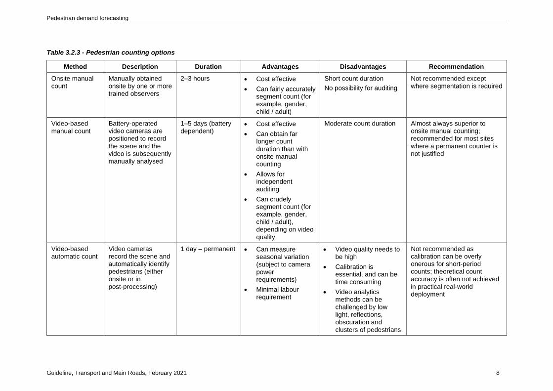
3.2.3 Count options

Four options for pedestrian counting are described in Table 3.2.3. In almost all circumstances, the

video-based manual count and permanent (automatic) count are likely to be the recommended

options. In some situations, it may be useful to obtain data that provide more specific information

about users, such as gender or age. Some collection methods allow for data to be segmented so that

sub-sets such as adult / child or male / female are identified.



Table 3.2.3 - Pedestrian counting options

Method Description Duration Advantages Disadvantages Recommendation

Onsite manual count

Manually obtained onsite by one or more trained observers

2–3 hours • Cost effective

• Can fairly accurately segment count (for example, gender, child / adult)

Short count duration

No possibility for auditing

Not recommended except where segmentation is required

Video-based manual count

Battery-operated video cameras are positioned to record the scene and the video is subsequently manually analysed

1–5 days (battery dependent)

• Cost effective

• Can obtain far longer count duration than with onsite manual counting

• Allows for independent auditing

• Can crudely segment count (for example, gender, child / adult), depending on video quality

Moderate count duration Almost always superior to onsite manual counting; recommended for most sites where a permanent counter is not justified

Video-based automatic count

Video cameras record the scene and automatically identify pedestrians (either onsite or in post-processing)

1 day – permanent • Can measure seasonal variation (subject to camera power requirements)

• Minimal labour requirement

• Video quality needs to be high

• Calibration is essential, and can be time consuming

• Video analytics methods can be challenged by low light, reflections, obscuration and clusters of pedestrians

Not recommended as calibration can be overly onerous for short-period counts; theoretical count accuracy is often not achieved in practical real-world deployment



Method Description Duration Advantages Disadvantages Recommendation

Signalised intersection quasi-counts

Apply expansion factor to STREAMS signal logs to estimate demand

Permanent • Cost effective

• Long time series

• An approximation of pedestrian demand

• Inaccurate at high demand sites (>20 pedestrians in 15 minutes)

May be useful for signalised intersections where no counts are available and demand is low

Permanent (automatic) count

Permanent systems installed to provide continuous counts (sensors include passive and active infrared detectors, video and 3D cameras)

Permanent • Can measure seasonal variation

• Accuracy >90% for high-quality systems installed in suitable locations

• Minimal labour requirement once installed

• Can be costly ($4000+)

• Cannot segment count (for example, gender, child / adult)

• Can be inaccurate under adverse weather or crowding conditions (technology dependent)

• Multiple devices may be required for large areas such as intersections

Recommended where high-quality, long duration data are warranted



Signalised intersection quasi-counts may be an option where there are inadequate resources to

commission counts at a signalised intersection. In this method, the STREAMS signal logs are used as

a proxy for pedestrian demand. Such logs are limited – they do not directly count pedestrians;

however, as described in Pedestrian Demand Forecasting Methods Guidance – Technical Report 2:

STREAMS validation (email [email protected] to request a copy of this document), an

approximate level of demand can be estimated as follows:

1. pedestrian phase call-ups from the STREAM cycle analyser file are aggregated into

15-minute bins

2. an expansion factor of 2.3 is applied to these 15-minute total call-ups (the expansion factor of

2.3 was found to apply fairly consistently across the seven mid-block pedestrian operated

signals described in Technical Report 2, and at different demand levels), and

3. the expanded 15-minute totals are summed to provide a daily demand estimate.

This estimate is appropriate only at signalised intersections with low to moderate pedestrian demand;

where the 15-minute pedestrian count is likely to regularly exceed 20 pedestrians; the expansion will

tend to underestimate true pedestrian demand. For sites at or below this demand, the expansion is

likely to be accurate to within ±25%.

3.3 Count specification

In undertaking counts, the following minimum specification should be used:

• counts should extend over busy periods on at least three days

• survey location should be clearly indicated, including providing an aerial image or photograph

of the site with mark-up to indicate the area in which counts were undertaken and the

movements (if classified)

• classification may vary, depending on the count purpose, but will likely include

mode (pedestrian, cyclist, scooter and, possibly, mobility-aided) as a minimum and, possibly,

age (adult, child) and gender – the latter two are subjective and can be difficult to assess from

a video record with reliability

• counts should be classified by movement (including direction of travel), and

• counts should be provided in a maximum of 15-minute intervals.

Counts should be provided in a tidy structure where each variable forms a column and every row

represents an observation. An example of a tidy data structure is provided in Table 3.3(a) and an

inappropriate format in Table 3.3(b).

Note: In Table 3.3(a), each row has one count, with columns indicating the time period, intersection arm and

direction of travel. By contrast, in Table 3.3(b), there are four counts on each row. This structure can be more

difficult to process into databases and in batch processing and is not recommended. Non-proprietary,

machine-readable formats such as comma separated values (csv) are preferred to proprietary binary formats (for

example, Microsoft Excel™).




Table 3.3(a) – Example of tidy data structure (recommended)

Time starting Arm Direction Count

6:00 West North 5

6:00 West South 3

6:00 East North 8

6:00 East South 1

6:15 West North 7

6:15 West South 2

6:15 East North 9

6:15 East South 4

Table 3.3(b) – Example of wide data structure (not recommended)

Arm West East

Direction North South North South

Time starting

6:00 5 3 8 1

6:15 7 2 9 4

3.4 User perceptions and behaviour changes

In some cases, user perceptions will be useful to provide insight into shortcomings prior to

construction of a project or will provide additional insight afterwards. Moreover, the effectiveness of

treatments at encouraging new walking activity can be directly measured by asking users whether

they have changed their behaviour as a result of the treatment. Most important is to identify whether

(a) users would otherwise have travelled by a different mode of transport for their journey (that is, car,

public transport or bicycle) or (b) they are making all-new walking trips directly as a result of the

project.

The recommended method for identifying user perceptions is to conduct an intercept survey after

construction. This survey should be conducted at relatively busy times (to maximise sample sizes) and

seek to interview, as a general guide, around 100 pedestrians. Survey times should, as much as

feasible, be representative of the user mix – for example, a weekday morning to capture commuting

walking and weekend morning to capture recreational walking.



4 Factoring

4.1 Introduction

In this method, pedestrian counts are obtained prior to construction and these are factored up using

indicative diversion rates from other completed projects to provide an estimate of the post-construction

demand. This method consists of three steps:

1. obtain counts of existing pedestrians at the site(s) over at least three typical days between

6am–6pm (or longer)

2. estimate the split between transport and recreation walking activity expected on the proposed

facility, and

3. factor up the observed demand using diversion rate factors described in this section.

Each of these steps is described in the following sections.

4.2 Obtain pre-construction counts

Pedestrian counts should be obtained at the site over a minimum of three typical days as described in

Section 3.2. Public holidays and school holidays should be avoided, as should days of extreme

weather conditions; some weather variability (such as light showers) on at least one of the days is

acceptable, noting that, in most locations, inclement weather is not atypical.

Whether the counts should be obtained over three weekdays or over a combination of weekdays and

weekend days will depend upon the primary motivation for the project:

• projects that are motivated primarily to provide for commuters or school students should use

three weekdays of counts, and

• projects motivated by recreational use should have at least one weekend day and possibly up

to three weekend days if the project is anticipated to be used only on weekends.

The count days need not be sequential, although, for logistical reasons, this is likely to be the most

practical choice.

In most cases, the most practical and cost-effective counting method will be manual counts from video

recordings. Doing so makes the long duration (minimum 36 hours, assuming 12 hours per day across

three days) of counts practical and provides a means to audit the count when required. Automated

computer vision-based algorithms are generally not recommended as the quality of video is generally

high and calibration times overly onerous for short-period counts.

4.3 Purpose split

The walking trip purpose split is required to estimate the diversion rates (Step 3 in Section 4.1 of this

guideline). Walking trips are divided into two groups:

1. transport: walking to work, personal business (for example, hairdresser, bank), shopping, to

restaurants or cafes, or to visit friends or relatives, and

2. recreation: any walking activity where the act of walking is itself the purpose – this would

include dog walking.

If the trip involves multiple purposes (for example, walking for both exercise and for a transport

purpose, such as shopping, or a trip to a café), the trip is treated as having a transport purpose. This

approach is consistent with purpose hierarchies assumed in travel surveys.



Typical pedestrian walking purpose splits for a range of suburban and regional footpaths and shared

paths are given in Table 4.3. There will be instances where the expected purpose split will be

significantly different from the values listed in Table 4.3; for example, in a central business district, the

transport purpose split on weekdays will very likely be higher than the range stated in this table.

Indeed, analysis of Queensland Travel Survey data from 2017–2019 suggests that only 24% of

walking trips are for a recreation purpose. The practitioner should make an assessment based on the

local context as to the most appropriate value.

The purpose splits by day of week in Table 4.3 add to above 100%. This reflects the

average-of-averages approach used in their derivation. Practitioners should select a value in one cell

about which they have most confidence and then derive the remainder; for example, if there is high

confidence that the weekday transport purpose split is likely to be close to the typical value in

Table 4.3 (that is, 37%), the recreation split should be set at 100 – 37 = 63%.

One overall weighted purpose split should be estimated across the analysis period. If the analysis

period is only weekdays or weekend days, no weighting is required. If a combination of weekdays and

weekend days is used, an overall weighted purpose split should be calculated as follows:

• Calculate the average weekday (AWT) and weekend (AWE) demand

• The weekday weighting WAWT is:

𝑊𝐴𝑊𝑇 =5𝐴𝑊𝑇

5𝐴𝑊𝑇 + 2𝐴𝑊𝐸

• The weekend weighting WAWT = 1 – WAWT.

Table 4.3 – Typical purpose splits by day of week

Day of week Transport Recreation

Weekday 37%

(24 – 51%)

70%

(58 – 83%)

Weekend 18%

(8 – 28%)

86%

(77 – 94%)

1. Values in brackets are 95% confidence intervals.

2. Values are derived from intercept surveys of pedestrians after construction of 20 projects in Australia.

3. Practitioners should ensure the total purpose split is equal to 100% on any weekday or weekend.



4.4 Diversion rates

Diversion rates are the proportion of users after construction that are estimated to have changed their

behaviour as a result of the project. There will be three potential user responses:

1. pre-existing:

a. these users were already walking prior to construction; depending on the project they

may have already been walking along the project corridor (for example, if the project

involves upgrading an existing facility) or have used some other route if the corridor is

altogether new

2. mode diversion:

a. previously used a private vehicle (usually car), either as a driver or passenger, and/or

b. previously used public transport, and

3. induced:

a. new walking trips that would not otherwise have occurred in the absence of the

project.

In most projects, the majority of pedestrians are likely to be pre-existing – they may, however, be

attracted to use the project in preference to another, more circuitous or unattractive, pre-existing route.

The proportion diverting from motorised modes (private vehicle or public transport) will depend on

(a) the proportion of transport versus recreation demand (higher levels of transport demand will lead to

higher diversion), and (b) the relative attractiveness of the motorised modes. In many suburban and

regional situations, the public transport mode shares will be low and diversion from public transport will

be negligible. Conversely, in major city centres, there will be higher pre-existing public transport mode

shares and lower car shares (due to congestion and parking limitations). Indicative diversion rates are

shown in Table 4.4 and illustrated in Figure 4.4. These diversion rates are based on intercept surveys

of pedestrians on new shared paths, footpaths and road crossings in Queensland. The practitioner

should select values appropriate to the local context, taking into account factors such as:

• pre-existing car and public transport mode shares along the corridor – for example, areas with

negligible public transport use would be expected to have no mode shift from public transport

• the scale of the project relative to the existing condition – large, high-quality projects where

there was previously very poor provision may have a greater mode shift and induced travel

effect, and/or

• local amenity of walking – projects in areas of significant natural features (for example, parks,

along waterfronts) or otherwise attractive to walking near residential or employment land uses

may induce more recreation walking than projects in less amenable surrounds.



Table 4.4 – Typical diversion rates

Trip purpose

Diversion Transport Recreation

Pre-existing 69%

(50–88%)

67%

(58–75%)

Mode shift from car 24%

(14–34%)

5%

(2–8%)

Mode shift from PT 19%

(3–36%)

0%

Induced 0%

(21–39%)

30%

1. Values in brackets are 95% confidence intervals.

2. Values are derived from intercept surveys of pedestrians after construction of 20 projects in Australia.

Figure 4.4 – Diversion rates for pedestrian infrastructure projects based on purpose split



The diversion rates can be converted into uplift factors for the purpose of forecasting additional

walking activity that the project may generate as follows:

𝐷 =𝐷0

𝐷𝑅𝑃𝐸

where:

𝐷 = forecast demand

𝐷0 = observed (pre-construction) demand

𝐷𝑅𝑃𝐸 = pre-existing diversion rate

For example, if the observed pre-existing demand at a location is 100 pedestrians per day, and all are

assumed to be recreational travellers, then the forecast demand would be:

𝐷 =100

0.67= 149

4.5 Calculation method

The procedure is illustrated with the following example:

1. A new pedestrian crossing is proposed at a mid-block location.

2. Pedestrian counts within 50 m of the location over two weekdays found an average weekday

crossing demand of 100 pedestrians. Crossing demand on a single weekend day was

observed to be 30 pedestrians. The average day demand (𝐷𝐴𝐷𝑇) is:

𝐷𝐴𝐷𝑇 =100 × 5 + 30 × 2

7= 80

3. The location is a fairly typical suburban area dominated by residential dwellings interspersed

with modest mixed-use development. It is assumed the purpose split on weekdays is

70% recreational and increasing to 90% on weekends (Table 4.3). The weighted purpose split

is:

𝑊𝐴𝑊𝑇 =5 × 100

5 × 100 + 2 × 30= 0.893

𝑊𝐴𝑊𝐸 = 1 − 0.893 = 0.107

𝐴𝑣𝑒𝑟𝑎𝑔𝑒 𝑟𝑒𝑐𝑟𝑒𝑎𝑡𝑖𝑜𝑛 𝑠𝑝𝑙𝑖𝑡 = 0.893 × 0.7 + 0.107 × 0.9 = 0.721 (72%)

𝐴𝑣𝑒𝑟𝑎𝑔𝑒 𝑡𝑟𝑎𝑛𝑠𝑝𝑜𝑟𝑡 𝑠𝑝𝑙𝑖𝑡 = 1 − 0.721 = 0.279 (28%)

4. Obtain a purpose-weighted uplift factor (UF) from the diversion rates and the average purpose

splits:

𝑈𝐹 =1

𝐴𝑣𝑔 𝑟𝑒𝑐. 𝑠𝑝𝑙𝑖𝑡 × 𝐷𝑅𝑃𝐸(𝑟𝑒𝑐) + 𝐴𝑣𝑔 𝑡𝑟𝑎𝑛𝑠. 𝑠𝑝𝑙𝑖𝑡 × 𝐷𝑅𝑃𝐸(𝑡𝑟𝑎𝑛𝑠)

𝑈𝐹 =1

0.721 × 0.67 + 0.279 × 0.69= 1.48

5. Multiply the observed (pre-construction) demand by the uplift factor to obtain the demand

forecast:

𝐷 = 80 × 1.48 = 118



In other words, for this project, the average daily demand is forecast to increase from

80 pedestrians per day prior to construction to 118 afterwards – an additional demand of

38 pedestrians per day.

5 Comparison methods

5.1 Background

Comparison methods represent the simplest means of forecasting demand for a pedestrian project. In

this approach, the possible demand is estimated from one or more other similar sites. The counts at

another site can be derived in one of two ways:

1. the practitioner can commission counts at one or more existing similar sites and infer from

these counts the likely demand at the project site; for example, if the project is a mid-block

pedestrian-operated signal across an arterial road in a predominantly residential area, counts

could be obtained at existing pedestrian operated signals in similar locations, and/or

2. an existing counts database can be used to identify similar sites and deduce the likely

demand.

Advice on counting for option 1 is provided in Section 3.2. The remainder of this section describes an

existing counts database.

5.2 Counts database

An online database of pedestrian counts obtained in Queensland is available at

https://pedtools.com.au/forecasts. The database tab in this tool is an implementation of the database

described in this section.

This database enables practitioners to search among 445 counts obtained since 2009 across a range

of contexts including signalised intersections, paths and zebra crossings. The data were collated from

counts commissioned in Transport and Main Roads and local governments and includes both

short-period (one day, 6am–6pm) and long-period (automatic) counts.

Practitioners can filter the database by criteria:

• facility type: signalised intersection, sign-controlled intersection, paths, bridges, roundabouts,

zebra crossings and mid-blocks, and/or

• local government area.

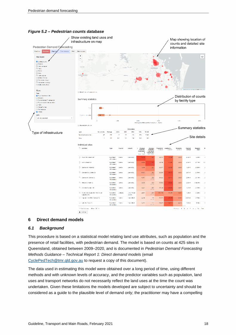
Statistics are provided for the average and median weekday (6am–6pm) and peak hour demand, as

well as the interquartile range and 95% confidence intervals (Figure 5.2). Tables are provided listing

each individual site and the population, employment and school students within a 2000 m catchment.

In combination, the practitioner can use these data to estimate the plausible demand for a notional

project. Given the inherent variability across sites, and the interday variability present within the

counts, practitioners are advised to use the median values as initial guidance, then consider varying

their estimates within the confidence intervals provided.




Figure 5.2 – Pedestrian counts database

6 Direct demand models

6.1 Background

This procedure is based on a statistical model relating land use attributes, such as population and the

presence of retail facilities, with pedestrian demand. The model is based on counts at 425 sites in

Queensland, obtained between 2009–2020, and is documented in Pedestrian Demand Forecasting

Methods Guidance – Technical Report 1: Direct demand models (email

[email protected] to request a copy of this document).

The data used in estimating this model were obtained over a long period of time, using different

methods and with unknown levels of accuracy, and the predictor variables such as population, land

uses and transport networks do not necessarily reflect the land uses at the time the count was

undertaken. Given these limitations the models developed are subject to uncertainty and should be

considered as a guide to the plausible level of demand only; the practitioner may have a compelling




argument as to why demand at a subject site will be significantly less or greater than predicted by this

model.

6.2 Model

The model is a generalised linear model with negative binomial errors and a log link function. The

model predicts weekday pedestrian demand between 6am–6pm; the model coefficients are shown in

Table 6.2(a). The key characteristics of this model are:

• higher commuting walking to work and public transport mode shares are associated with

higher pedestrian demand

• higher household income is associated with slightly lower pedestrian demand

• higher median age is associated with higher pedestrian demand

• proximity to a school is associated with higher pedestrian demand

• proximity to, and higher areas of, parks or retail facilities are associated with higher pedestrian

demand, and/or

• infrastructure such as footpaths (at mid-blocks), roundabouts and sign-controlled intersections

are associated with lower pedestrian demand than off-road paths, signalised intersections and

zebra crossings.

The marginal effects for this model are generally plausible; for example, for a shared path and

average parameters, as shown in Table 6.2(b):

• increasing the walk mode share to work from 10% to 20% will increase weekday pedestrian

demand by 433 pedestrians per day

• increasing public transport mode share to work from 10% to 20% will increase weekday

pedestrian demand by 190 pedestrians per day

• increasing the distance of the nearest school from 300 m to 1000 m will reduce weekday

pedestrian demand by just under 100 pedestrians per day

• areas with a median weekly household income of $1000 will have pedestrian demand around

117 pedestrians per day higher than areas with median weekly demand of $2000, and/or

• areas with a median age of 45 years will have pedestrian demand around

120 pedestrians per day higher than areas with a median age of 35 years.



Table 6.2(a) – Direct demand model

Predictor Coefficient

(Intercept) 3.649***

(0.000)

walk.share.wgt 9.157***

(0.000)

pt.share.wgt 6.421***

(0.000)

hh.income.wgt -0.001***

(0.001)

median.age.wgt 0.056***

(0.000)

dist.school -0.703***

(0.000)

park.km2.wgt 2.7E-7

(0.117)

retail.km2.wgt 6.69E-6***

(0.001)

dummyFootpath -1.155***

(0.000)

dummyRbt -0.432**

(0.033)

dummySign -0.753***

(0.000)

Num.Obs. 425

AIC 5310.4

BIC 5359.0

Log.Lik. -2643.203

Values in brackets are p-values

* p <0.1, ** p <0.05, *** p <0.01



Table 6.2(b) – Variable description

Predictor Description Unit

walk.share.wgt Distance-weighted proportion of walking trips (as a sole mode) to work, based on 2016 Australian Bureau of Statistics (ABS) Census of Population and Housing

0–1

pt.share.wgt Distance-weighted proportion of public transport trips to work based on 2016 ABS Census of Population and Housing

0–1

hh.income.wgt Distance-weighted median household weekly income based on 2016 ABS Census of Population and Housing

$ (2016 prices)

median.age.wgt Distance-weighted median age based on 2016 ABS Census of Population and Housing

Years

dist.school Crowfly distance to the centroid of the nearest primary or secondary school

km

park.km2.wgt Distance-weighted crowfly distance to the nearest point of the nearest park multiplied by the park area

km³

retail.km2.wgt Distance-weighted crowfly distance to the nearest point of the nearest point of the nearest retail land use multiplied by the retail land area

km³

dummyFootpath Whether the count site is a footpath (that is, a walkway dedicated to pedestrians within a road-related area).

0 = not a footpath

1 = footpath

dummyRbt Whether the count site is at a roundabout 0 = not a roundabout

1 = roundabout

dummySign Whether the count site is at a roadway intersection that is sign-controlled (either give way or stop signs)

0 = not a sign-controlled intersection

1 = sign-controlled intersection

6.3 Implementation

To assist practitioners in the rapid use of this model, an online implementation is provided at

https://pedtools.com.au/forecasts under the Forecasting tab. In this implementation, the user drops a

marker onto the map at the project location and the model calculates the demand forecast, using the

model described previously. The practitioner is provided with a table indicating the demand and

95% prediction interval, along with the key land use characteristics.




Figure 6.3 – Direct demand model

The model is based on data of variable quality, the model fit is modest and many significant factors

likely to contribute to pedestrian demand are not explicitly accounted for, such as:

• population and employment

• size of nearby schools – that is, while the presence of a school and its proximity to the count

site is incorporated, the number of students is not

• the quality of the walking facility and amenity of the immediate surrounds (aside from the

presence of a park), and/or

• the presence of significant tourism-related pedestrian activity.

7 Worked example

This section illustrates the use of the procedures through a hypothetical example. In this example, the

practitioner is considering a zebra pedestrian crossing at two locations in Toowoomba:

1. Hume Street south of Stenner Street, adjacent to a local shopping centre and residential area,

and

2. Vacy Street west of Mirle Street, adjacent to a major shopping centre and school.

The practitioner is interested in assessing the site likely to have the highest pedestrian demand.

7.1 Comparison method

There are currently very few zebra crossings in the database; however, all are in suburban areas not

entirely dissimilar to the subject sites. The median weekday crossing demand for these sites is

134 pedestrians per day with a range from 117–339 pedestrians per day. The limited number of sites

in the database precludes estimating demand for the two sites in Toowoomba separately.



7.2 Factoring

Step 1: Observed demand

Assume pedestrian counts were obtained from 6am–6pm at each of the two subject sites over

three typical weekdays. Assume average weekday demand at Hume Street was 150 pedestrians / day

and, on weekends, was 100 pedestrians / day within 50 m of the potential crossing location. Further

assume the average weekday demand at Vacy Street was 200 pedestrians / day and

20 pedestrians / day on weekends.

Step 2: Purpose split

Assume on weekdays the demand at Hume Street is evenly split between transport and recreational

walking, on the basis that the local shopping centre will generate and attract transport walking activity.

On weekends, assume there is more recreational walking, such that 70% of pedestrian crossing

events are for recreation. Vacy Street pedestrian demand is likely to be dominated by school students

and those accessing the nearby shopping centre. Assume, on weekdays, that more trips are for

transport (80%), but that this share is much reduced on weekends (20%).

Step 3: Pre-existing walking

The zebra crossings are assumed to have only a marginal effect on walking activity; they are unlikely

to encourage mode shifting towards walking but may encourage pedestrians to cross at this location

as opposed to elsewhere along the street. Assume, at Hume Street, that 80% of crossing events for

recreation after the zebra crossing is installed would have occurred here anyway, and that 90% of

transport walking did similarly. A higher proportion is assumed for transport on the assumption that

these pedestrians are likely to be more time-sensitive and less likely to divert to use the crossing.

Assume the same pre-existing walking shares for the Vacy Street location.

Calculations

Using these assumptions and the procedure documented in Section 4, the average weekday demand

will be:

𝐷ℎ𝑢𝑚𝑒 =1

0.50 × 0.80 + 0.50 × 0.90× 150 = 176

𝐷𝑣𝑎𝑐𝑦 =1

0.80 × 0.80 + 0.20 × 0.90× 200 = 227

The average weekend demand will be:

𝐷ℎ𝑢𝑚𝑒 =1

0.30 × 0.80 + 0.70 × 0.90× 100 = 120

𝐷𝑣𝑎𝑐𝑦 =1

0.20 × 0.80 + 0.80 × 0.90× 20 = 24

Under these assumptions, the best estimate is that weekday demand will increase by 18% or

26 pedestrians/day at Hume Street and by 14% or 27 pedestrians/day at Vacy Street.

7.3 Direct demand

The direct demand model can only practically be implemented using the online tool at

https://pedtools.com.au/forecasts. Doing so gives the forecasts shown in Table 7.3. The model

estimates demand at Vacy Street of 342 pedestrians per day compared to 228 pedestrians per day at

Hume Street. There are a number of factors contributing to this higher estimated demand at




Vacy Street, of which the most significant are the much larger retail area within the catchment and

higher walking mode share for travel to work. The population is also higher than for Hume Street, but

total employment and school students are lower for Vacy Street.

Table 7.3 – Direct demand forecasts for example sites

Site

Hume Street Vacy Street

Weekday demand (6am–6pm)

Estimate 228 342

95% confidence interval

172–283 253–431

Catchment (within 2 km)

Population 95,054 139,694

Employment 18,105 4751

Students 6413 2718

Walking mode share to work

3% 8%

Retail floor area 2,069 m² 46,753 m²

7.4 Summary

The procedures provide three estimates for weekday demand:

1. the comparison method suggests demand of around 134 pedestrians per day, and a range

from 117–339 pedestrians per day

2. the factoring procedure suggests demand at Hume Street of 176 pedestrians per day

increasing to 227 pedestrians per day at Vacy Street, and/or

3. the direct demand procedure suggests demand at Hume Street of

228 pedestrians per day (with a 95% confidence interval of 172–283) and

342 pedestrians per day (95% confidence interval of 253–431) at Vacy Street.

In summary, the procedures appear to suggest demand at both sites will exceed

100 pedestrians per day and most likely be under 400 pedestrians per day, and the factoring and

direct demand procedures are consistent, suggesting Vacy Street will have higher demand than

Hume Street.

8 Conclusion

This guideline provides three procedures for forecasting pedestrian demand for new pedestrian

infrastructure. The procedures should not be considered as definitive predictors of demand but rather

reasonable indicators based on the current state of knowledge. The procedures are limited in

several ways:

• there are very few sources of high-quality, multi-day pedestrian counts from which to develop

forecasting procedures in Queensland

• detailed, up-to-date land use and pedestrian network spatial datasets covering all of

Queensland are limited



• pedestrian demand is associated with a complex association of local population and

socio-demographics, transport network and topography, land use types and distribution

among numerous other factors – disentangling these factors, especially with the data

limitations, remains an ongoing challenge, and

• the procedures are based on existing conditions in Queensland, where the pedestrian network

quality and extent is often limited. These procedures are likely to underestimate demand

associated with very substantial, widespread improvements in pedestrian infrastructure.

Given the limitations, practitioners should use these procedures as a guide and apply local knowledge

to adjust the forecasts as appropriate to the local context. Practitioners should undertake multiday

pedestrian counts to improve data quality, and that these data can be used to update and improve

these procedures over time.

Pedestrian demand forecasting

Documents

Transcript of Pedestrian demand forecasting