Peak Detection with Varian MS Workstation - Lotus...

Peak Detection with Varian MS Workstation

for Varian 220 and 240 GCMS

by: Randall Bramston-Cook Lotus Consulting 5781 Campo Walk Long Beach, Ca 90803 310/569-0128 [email protected]

February 12, 2010

Copyright 2010 Lotus Flower, Inc.

A primary application of chromatography is measuring concentrations of analytes in unknown matrices. After compounds are separated on a column, they are sent to a detector to measure their responses. Concentrations are a function of the detector signal, usually by an established linear relationship. A critical factor in maintaining good reproducibility and accuracy of measurements is proper assignment of peak responses above baselines. If peak start and end points are not set appropriately, peak response can be either too large or too small, compared with its true value, and can vary dramatically with replicate runs of the same sample. Varian MS Workstation1 for mass spectral data uses a powerful peak detection algorithm originally developed in 1968 with the Varian 200 Data System set up for data collection from multiple gas chromatographs, and has been continually enhanced through the years in Varian CDS 101/111, Varian Vista 401/402, Varian DS601/651/654 and Star Data Systems, and is now in MS Workstation2, with many new enhancements over the older programs. Correct calculation of a peak response involves some judgments to distinguish a real peak from noise, rising backgrounds, change in peak shapes from temperature and flow programming, unexpected disruptions in detector response from instabilities, and flow disruptions (from valve switches, for example). The Workstation, with preset parameter settings, can usually find “peaks” and assign an area or height, but sometimes these initial values do not match criteria that an experienced operator might have given. This reported value may not properly represent the true concentration of an unknown. Varian MS Workstation provides a number of user selectable parameters to tune peak detection to specific conditions in use. For example, when a high performance capillary column is employed that generates some very sharp peaks, the user can set up parameters readily to fully detect these sharp peaks and ignore baseline drift from temperature programming. At the other extreme, if peaks are broad from use of packed or megabore columns, settings can be employed to expect these broader peaks and ignore detector spikes. Fortunately, preset parameters in this Workstation are usually sufficient to pick out most peaks, albeit not always optimally, and provide a starting point for fine tuning settings to accurately work on subsequent runs of the same ilk without further adjustments. Varian MS Workstation performs automatic full storage of every chromatogram, with all raw data points, calibration data, and method parameters. Some factors involved in initial data collection - such as data rate, ionization parameters, tune parameters and chromatographic conditions - cannot be changed on this stored data after the original run. Others settings can be altered and their effects on a chromatogram can be visually inspected. Then this modified method can be saved and made available for use with subsequent samples to achieve better results without further intervention. 1 Varian MS Workstation has been undergoing improvements over the years, and some significant changes related to peak detection have been implemented in later versions. All discussions here apply to Version 6.9.2.

2 This document presumes that the reader has some familiarity with various screens and operations within Varian MS Workstation. Hints are provided for locating specific operations within the Workstation for the following discussion points, but precise steps are not listed and are assumed to be obvious to the reader.

The precise retention time is set by linear interpolation of points before and after the zero crossing.

Determination of Retention Time Varian MS Workstation establishes retention time of a peak by computing the zero crossover of the first derivative of the peak. It this value does not correspond to a collected data point, precise timing is determined by linear interpolation of points before and after the zero crossing. Retention Time Adjustments with Identification Reference Peaks Measurements in chromatography cannot be considered exacting, as random and systematic errors can introduce some variability in retention times (along with area measurements). To help correct for systematic deviations in retention times, certain compounds can be assigned as Identification Reference Peaks. Any movement in time of these peaks is detected and a correction based on this change is applied proportionally to all “non-reference” peaks, based on their relative retention to reference peaks. If multiple Identification Reference Peaks are assigned, then the new Expected Retention Times are proportioned based on their proximity to these reference peaks.

Retention time is determined by zero-crossing of the first derivative of a

chromatographic peak.

The derivative is generated by an appropriate digital filter across the peak

(see later discussions on Filtering).

Identification Reference Peaks always must be present in every sample and standard in a series, and must be the largest peak within the Search Window; typically internal standards are perfect candidates. Non-reference peaks are picked out as the closest peak to the Expected Retention Time, after time adjustment from a Reference Peak correction. With a run type of “Analysis”, the Compound Table in the Method is not altered as a result of these operations and Identification Reference Peaks are only used to pick out peak movement and properly identify analyte peaks. For a Calibration run type, retention times in the Compound Table are updated based on the newly located peak positions.

Compound Expected

Retention Time Measured

Retention Time Measured

Shift Correction

New Expected Retention Time

Peak A 9.374 ‐‐ +0.045 9.419

IRP #1 13.841 13.907 +0.066 ‐‐ ‐‐

Peak B 21.844 ‐‐ ‐0.015 21.829

IRP #2 26.752 26.816 ‐0.064 ‐‐ ‐‐

Peak C 35.395 ‐‐ ‐0.085 34.545

Multiple Identification Reference Peaks can provide time corrections over the whole chromatogram. New Expected Retention Times for unknown peaks are adjusted proportionally to their positions relative to adjacent reference peaks. This synthetic

example illustrates the corrections involved for two reference peaks.

Tim

e S

hift In

ject

ion

IRP

#1

IRP

#2

0

+0.10

-0.10

20 30 40 100

Pea

k A

Pea

k B

Pea

k C

44.25 44.50 44.75 45.00 minute

0

200

kCou

nts

StartSearch

End Search

StartIntegration

EndIntegration

RMatch

ERTEthyl Benzene

m&p Xylenes

Normal variations in chromatographic conditions can shift retention times

away from the expected locations. And adjacent peaks can be mislabeled and

wrong results are reported.

Proper use of Identification Reference Peaks can sense a shift in retention times and allow corrections to move the “anticipated” Expected Retention

Time over to the correct peak. The reference peak is off-scale to the left.

Misidentified as m&p Xylenes

44.25 44.50 44.75 45.00 minutes

0

200

kCou

nts

Start Search

End Search

Start Integration

EndIntegration

RMatch

ERT

Automatic Retention Time Updates and Timed Event Adjustments Retention times do not always hold their precise locations in chromatograms and can be expected to move a bit from run to run, especially after the chromatograph sits idle for an extended interval or a new column is installed. If they are not adjusted to the new times, peaks may be labeled with incorrect names, and serious errors in quantitation can occur. In a calibration series, a subtle change in retention time is adjusted automatically by locating the peak within the integration window that is closest to the expected retention time and then replacing the listed time with the newly established one in the method Compound Table.

Updates to retention times are NOT performed with Analysis run types (unknown samples), as every peak may not always be present here. When a multipoint calibration is performed, the last run in the series ought to be a midlevel standard so that the final retention time update is accomplished on sizeable peaks, and not on puny peaks where retention time may be skewed by noise, and not on the largest peak where retention times may be distorted from column or detector overload.

38.6 38.8 39.0minutes

0

200

kCo

un

ts

Time Events

StartSearch

EndSearch

StartIntegration

EndIntegration

FP ERT 38.6 38.8 39.0 minutes

0

200

kCo

un

ts

TimeEvents FP

StartSearch

EndSearch

StartIntegration

EndIntegration

ERT

The Expected Retention Time (ERT) listed in the compound table was

originally set to 38.766 minutes, and a Forced Peak (FP) timed event is

misaligned with the new peak. Computed area is completely wrong

with this invalid baseline.

After a Calibration run type is executed, the retention time in the

compound table is updated with the true apex value (38.854 minutes), and all associated timed events are also

adjusted with the time change. Integration and Search windows are altered as well, now centered on the

peak acme.

Peak Simulations Shape of typical chromatographic peaks (red trace) can be approximated by a Gaussian distribution (shown in blue), as displayed to the right.3 Using this mathematical model, various data treatments available in Varian MS Workstation, such as data collection rates and smoothing, can be simulated and displayed. In discussions following, 600 points on a Gaussian curve are generated in Microsoft Excel to study various effects on peak processing. Noise is imitated by generating a series of random numbers within a specified range and then plotted.

Artificial peaks are created by adjusting Gaussian points to relate to the noise numbers produced. Two closely spaced peaks are used to look at effects of various parameters on resolution of the two, especially when these peaks are combined with random noise numbers.

3 Both actual data and simulated numbers are presented in this monograph to illustrate discussions about peak processing. Synthetic numbers are typically presented in blue graphs and real data are displayed in red.

Normal chromatographic peaks are nearly Gaussian in shape.

38.80 38.90 39.00minutes

0

150

kCo

un

ts

Noise is simulated by plotting a group of random numbers.

Overlapping peaks are created from Gaussian distributions, with

a 70% valley penetration.

The doublet peak structure is mathematically combined with the random noise to create a data set

closely resembling real peaks near their detection limits.

Definition of Terms µScan Point – This is a single spectrum scanned from low mass to high and becomes the raw data used for all further data processing. Scan Point – µScans are averaged together based on Scan Time or µScans Averaged. If Scan Time is specified, the number of µScans per Scan increases across the peak to keep the time interval constant. If Minimum # of µScans is checked, the scan rate increases across the peak. The choice becomes a trade-off between spectral quality (for Scan Time) and chromatographic peak quality (for Minimum # of µScans). Bunched Point – Scans are averaged together to provide ideally 10 to 20 Bunched Points across the top of a peak, based on the Expected Peak Width. Bunched points are used only for peak detection and not for peak integration. They are not displayed. Interpolated Point – Computer generated points for peak detection that are midway between adjacent Bunched Points, used to increase the number of points to find the correct start and end points of a peak when insufficient Bunched Points are collected. These points are only used for peak detection and baseline assignment and not for peak integration. They are not displayed.

Data Collection Rate Varian ion traps operate by storing all ions eluting from a chromatographic column within a specific mass range. Then these ions are ejected out of the trap to the detector with a ramping RF field, at a rate 5,000 to 10,000 u/sec over the scan range, to yield mass spectral raw points, labeled as µScans. Since these µScans often are generated faster than is required for most peaks, they can be averaged together to help reduce noise and to generate better quality spectra. These averaged data points are then stored in a .SMS or .XMS data file for post-run peak processing and are visible in chromatographic and spectral displays. This data bunching rate applies to the whole segment, and can be altered in other segments if needed. The rate that these data points are collected is a function of mass scan range, number of scan segments, tune type (where spectra are adjusted to match specific criteria), scan type (Full, MS/MS, SIS and µSIS), and, for the Varian 240/4000, scan mode (Normal, Fast, or Fastest).

Parameter entries for Varian 240/4000 to set Data Rate.

With the Varian 220/2200, the entry of scan time sets the µScans Averaged. Data rate is computed by taking the reciprocal of the Scan Time. For example, for a Scan Time of 0.24 sec/scan, the Data Rate is 4.17 Hz. And the Varian 240/4000 allows entry of either Scan Time or µScans Averaged, with the other computed based on all of the criteria listed above and then shown grayed out. The Data Rate displayed is based on the resulting Scan Time.

Data rates for Varian Ion Traps are dependent on conditions used for the mass spectrometer. Typical conditions for measuring toxic compounds by EPA Methods 524.3, 624B, 8260 and Method TO-15 are employed for the data rate listings below:

Mass Range 35-300 m/z

Steps in Tune Segments 4

4 Displayed data rates are for the specified mass range and segment count. Other settings for these settings will result in differing scan times and data rates. 5 These µScans Averaged settings are the maximum allowed values.

Data Rates4 for Varian 220/2200 GCMS

Scan Time (sec/scan)

µScans Data Rate

(Hz)

0.24 1 4.17

0.48 2 2.08

0.95 4 1.05

1.89 8 0.53

3.76 16 0.27

5.00 21 0.20

Data Rates4 for Varian 240/4000 GCMSScan Mode - Normal Fast Fastest

µScans Averaged


Data Rate (Hz)


Data Rate (Hz)


Data Rate (Hz)

1 0.34 2.94 0.31 3.23 0.08 12.50

2 0.67 1.49 0.62 1.61 0.16 6.25

4 1.34 0.75 1.24 0.81 0.32 3.13

8 2.68 0.37 2.47 0.40 0.63 1.59

16 5.36 0.19 4.94 0.20 1.25 0.80

32 10.71 0.09 9.88 0.10 2.49 0.40

64 21.42 0.05 19.75 0.05 4.98 0.20

89 29.795 0.03 - - - -

97 - - 29.935 0.03 - -

99 - - - - 7.705 0.13

Parameter entry for Varian 220/2200 to set Data Rate.

Width½ Height = 3.6 sec

1 µScan Averaged

2 µScan Averaged

3 µScan Averaged

5 µScan Averaged

10 µScan Averaged

33.6 33.9 34.2 minutes


1 µScan Averaged

2 µScan Averaged

3 µScan Averaged

5 µScan Averaged

10 µScan Averaged

33.6 33.9 34.2 minutes

240 ‐ Normal Scan Mode uScans

Averaged Points above Half Width

Relative Area

Relative Peak Height

1 20 1.00 1.00

2 13 0.97 0.99

3 7 0.95 0.99

5 3 0.87 0.89

10 2 0.87 0.79

240 ‐ Fast Scan Mode uScans


Relative Area


1 22 1.00 1.00

2 10 0.99 0.97

3 7 0.99 0.95

5 5 0.94 0.77

10 2 0.89 0.74

Data rates can have a major impact onpeak shapes and displayed noise. The goalfor optimum detection is to maintain between10 and 20 data points across the top of thepeak. With a Normal scan mode with theVarian 240, peak areas remain consistentover a narrow range of µScans Averaged, aswell as peak heights. Peaks displayed at leftdo not any smoothing functions applied.Noise can be suppressed with Mean orSavitsky-Golay smoothing.

As expected with a limited massrange and similar data rates as with theNormal Scan Mode above, the FastScan Mode exhibits nearly the samepeak characteristics over a range ofµScans Averaged.

240 ‐ Fastest Scan Mode uScans


Relative Area


1 63 1.00 1.00

2 39 1.00 0.99

3 26 1.00 0.99

5 15 0.98 0.98

10 8 0.97 0.97

220 ‐ Segment Setpoint Seconds/ Scan

Points above Half Width

Relative Area


0.3 12 1.00 1.00

0.4 8 0.98 1.00

0.5 7 0.96 0.99

0.7 5 0.94 0.94

1.0 3 0.92 0.92

2.0 1 0.83 0.80

The Fastest Scan Mode isimplemented to accurately pick up verysharp chromatographic peaks (< 1second peak width). However, with“normal” peak widths (typically 3seconds), the range of µScans Averagedgiving equivalent peak areas is muchwider than with the other modes.However, noise is dramatically higherwith low settings. Smoothing actions(see below) are needed to curb thisdegradation of the peak shape and helpin making peak detection for the full peaka bit easier.


1 µScan Averaged

2 µScan Averaged

3 µScan Averaged

5 µScan Averaged

10 µScan Averaged

33.6 33.9 34.2 minutes

The Varian 220 parameter entry fordata rates differs somewhat from thosewith the Varian 240. Available choicesfor the 220 are only in units ofSeconds/Scan, and yet demonstratesimilar consistencies for a narrow range,with severe degradation if set toocoarsely. Performance matches resultswith 240 - Normal Scan Mode, asanticipated.


0.3 seconds/scans

0.4 seconds/scan 0.7 seconds/scan

1 second/scan

2 seconds/scan

0.5 seconds/scan

35.9 36.3 36.7 minutes

Data points in a chromatogram are visible in MS Data Review screens when the time axis is expanded sufficiently to view them. To achieve full value of the peak height, at least 10 points should span across the top of the peak above the width at half height. Fewer points will degrade the value for the highest point, but remarkably peak area remains intact.6

Integration Window Each identified peak has an assigned window where all integration must take place. Any portion of the chromatogram outside this window is not considered for that peak, with the exception of the noise window. The position of the window is centered on the expected retention time of the peak in the Compound Table. A window for each identified peak is assigned in Method MS Data Handling Compound Table Integration Method. The preset value is ± 0.25 minutes. Size of this window can be readjusted through MS Data Review on archived .SMS files, and its absolute location relative to the peak can be changed by correcting the expected retention time for the peak. This parameter positioning should be adjusted to correlate with the chromatography. A window too narrow for the peak can dramatically alter peak integration and noise assessment. A window too wide can effect a switch in peak assignment, especially for Identification Reference Peaks, to an adjacent peak now within the window.

6 Data presented in this table are generated from synthesized data, without consideration of noise.

Points across Peak Width ½ ht

Relative Peak Area


∞ 1.00000 1.000

17 0.99999 0.998

9 0.99998 0.993

5 0.99997 0.971

3 0.99986 0.950

2 0.945 0.500

Data points defining the peak are displayed by expanding the time axis

until these points become visible.

29.20 29.30 29.40minutes

0

30

kCou

nts

Width½ ht

48.0 48.2 48.4minutes

0

200

kCou

nts

StartIntegration

EndIntegration

48.0 48.2 48.4minutes

0

200

kCou

nts

StartIntegration

EndIntegration

Integration Window = ±0.25

Integration Window = ±0.10

Computation of Noise for Peak Detection Peaks are separated from uninformative noise by assessing the level of noise surrounding identified peaks. Then a peak start is sensed when the signal exceeds this established noise. And peak end is perceived when the back of the peak approaches this noise. The type of noise is computed and reported based on the user’s choice in Calculations Setup in the Method. Peak-to-Peak is simply the difference between high and low data points within a 5-data point window (as shown below). Root-mean-square (RMS) noise is an average of two 10-data points windows - one before the apex and one after. RMS noise is computed by the formula:

···

Synthetic chromatogram provides data points to illustrate the measuring of noise levels.

Root Mean Square (RMS) is applied to sets of ten points across +/- (50 data rate) points from the apex of the synthetic chromatogram. Results then are sorted from low to high to the peak apex, and then high to low to the end. The middle 50% of the data points are excluded, and the numerical average of the two middle points of the remaining for each side of the apex becomes the basis for the RMS noise: 30.4.

30.6 30.2

Peak-to-peak noise (P-P) is computed by taking the difference between the high and low values within sets of five data points across +/- (50 data rate) points of the synthetic chromatogram. The differences are then sorted from low to high. 50% of the high ones are excluded and middle point of the remaining becomes the basis for the P-P noise: 77.

77.0

A peak for 3 ppt Benzene (300 ml loading, at 78 m/z, 11-point Saviksky-Golay smoothing) is used to illustrate how regions are shown when computing RMS Noise.

The noise areas used for noise assessment can be visually displayed through MS Data Review Plot Chromatograms and Spectra, then right-click mouse anywhere in the chromatogram pane to select Chromatogram Plot Preferences from the menu. Choosing “Noise” Noise Marker Appearance - Edit Color and Font will pull up a window with a check box to Draw Noise Boxes.

Then the peak apex is picked with the mouse pointer and Calculate S/N (Plot 1) is chosen, resulting in the areas used to be highlighted. The noise level found is displayed as “N” at the peak apex. This noise value is used for both peak detection and computation of Signal-to-Noise for the peak. The search for the lowest noise interval can extend outside the Integration Window, but will not cross segment changes, such as switching between Full Scan and MSMS. If insufficient space is allotted for this noise evaluation, the window is allocated up to the change. The Noise areas used for peak detection cannot be displayed in the MS Data Review View Results Chromatogram Pane, as these are often outside the Integration Window and would not be available for display here.

The steps to enable display of the chromatographic regions involved in setting the noise value for peak triggering are shown.

Expected Peak Width

The peak detection algorithm is set to be able to sort out unexpected peak shapes. For example, if peaks are anticipated to be sharp from “fast” chromatography, then broad baseline drift or background humps should be ignored. At the other end of the scale, if peaks are predicted to be wide, then sharp “spikes” are to be considered as disruptions, and thus disregarded. The precise setting for this parameter is not critical as Varian MS Workstation readily locates a peak even when expected peak widths do not correlate precisely with the actual widths of detected peaks. The preset value is 4.0 sec. An appropriate entry can be

found in Results View when Peak Width is added.

Detection of Peak Start with Slope Sensitivity Precise details of the peak detection algorithm in Varian MS Workstation are proprietary. The concepts discussed here are intended to provide a basic understanding of this process to improve the quality of the final results. User-selectable parameters for peak detection can have major impacts of the appropriateness of locating peak start and end points. After a chromatogram is run, its first derivative is performed7, using Cluster points, to determine peak starts. Based on the Noise threshold from the Noise Monitor interval prior to the start of the run and the Initial S/N Ratio, a peak start point is triggered when the derivative value first exceeds this value. This action point is:

Slope Sensitivity can be adjusted for individual peaks for optimum settings. The available range of values is 1 to 256.

7 Displayed derivatives of real data are generated through Microsoft Excel after conversion of raw data by ASCII operations.

The region at the front side of the derivative shown above illustrates locations for the

trigger point at 5 X Noise and actual Peak Start.

Noise Threshold

Trigger Point

Peak Start

A peak for 3 ppt V Toluene is used as an example of the peak detection process.

The last 60 Cluster Points prior to this trigger point are examined backwards to find a local minimum, which is then taken as the Peak Start. This step ensures that the true peak start is determined into the preceding noise and the computed area includes an area slice under the whole peak that would have been excluded if the peak start had been set at the trigger point. To illustrate the process for peak detection, several case studies demonstrate how expected peaks are reported and undesired peaks are ignored. If very narrow peaks are anticipated, then appropriate parameters, specifically expected Peak Width and Signal-to-Noise, need to be set to pick out the sharp peaks and disregard baseline drifts and unexpected broad peaks. Then when the derivative of the signal is performed, the target peak is properly detected and the broad “baseline drift” is ignored. With judicious choice of Expected Peak Width (0.5 sec) and Signal-to-Noise (5), only the sharp, narrow peak breaks the Signal-to-Noise Threshold; the broad peak does not come close to the Trigger level and is disregarded and not reported.

The derivative of this chromatogram readily picks out the narrow peak as it easily

exceeds the trigger point. The broad peak barely breaks the Noise threshold

and is not detected.

Noise Threshold

5 × S/N Trigger

A very narrow peak is synthesized along with a broad peak. With an expected Peak

Width of 0.5 sec, the narrow peak is targeted and the broad peak will be treated

as “uninteresting” baseline drift.

Peak Width = 0.1 sec

Peak Width = 8 sec

Peak End point is set when the derivative signal returns into

the Noise Threshold window.

PeakEnd

Noise Threshold

Then, when broad peaks are anticipated, expected Peak Width is widened to match the desired peak, and the consequential averaging often completely suppresses narrow peaks, as noise, and boosts detection of the wider target peak.

Detection of Peak End Peak end is detected when the derivative level returns into the Noise Threshold window. If this signal promptly zooms in a positive direction, then a fused peak is detected and a judgment is made with TAN% to determine if the rider peak requires a perpendicular drop to baseline or a tangent skim (see discussions below).

5 × S/N

Noise Threshold

Trigger

A derivative of the chromatogram, with a WI=8, gives a different sense to possible peak starts, as the narrow peak is hardly sensed, and noise on the broad peak is radically suppressed and its derivative

readily exceeds the threshold.

When broad peaks (width @ ½ height of 8 sec) are expected, the expected Peak Width can be set to match their widths (WI=8) and

sharp peaks will melt into the noise.

Peak Width = 8 sec

38.75 38.85 38.95 minutes

0

25

MC

ount

s StartIntegration

EndIntegration

Major peak for Toluene, 100 ppbV, 300 ml loading, at 91 m/z,

raw data (no smoothing), measured peak width - 3.4 sec,

Slope Sensitivity - 4, Expected Peak Width - 4 sec.

Interaction of Expected Peak Widths and Slope Sensitivity Effects of Expected Peak Width and Slope Sensitivity on area counts are studied with a Toluene peak at both high and low concentrations. Each chromatogram is opened in MS Data Review and the two parameters are varied over wide ranges. Areas are normalized to the correct area. This series shows how these two parameters have wide latitude in values for major peaks. However, small peaks approaching the noise level have more constraints on adequate values, without some manual interventions discussed below. Data smoothing helps widen the choices for these parameters without severely impacting computed areas.

Expected Peak Width (sec.)

0.5 1 2 4 8 16 32 64

Slo

pe

Sen

siti

vity

1 0.584 0.585 0.612 1.000 1.000 0.998 0.000 0.000

2 0.584 0.585 0.612 1.000 1.000 0.998 0.000 0.000

4 0.584 0.585 0.612 1.000 0.998 0.998 0.000 0.000

8 0.584 0.584 0.612 1.000 0.998 0.998 0.000 0.000

16 0.584 0.584 0.612 0.999 0.999 0.998 0.000 0.000

32 0.584 0.584 0.612 0.998 0.999 0.998 0.000 0.000

64 0.582 0.584 0.612 0.998 0.998 0.998 0.000 0.000

128 0.581 0.583 0.612 0.998 0.998 0.998 0.000 0.000


0.5 1 2 4 8 16 32 64

Slo

pe

Sen

siti

vity

1 0.175 0.174 0.196 0.606 0.605 1.050 0.000 0.000

2 0.162 0.181 0.196 0.606 0.603 1.000 0.000 0.000

4 0.051 0.173 0.196 0.606 0.603 1.076 0.000 0.000

8 0.361 0.173 0.192 0.606 0.647 1.038 0.000 0.000

16 0.000 0.000 0.174 0.475 0.611 0.869 0.000 0.000

32 0.000 0.000 0.000 0.164 0.439 0.756 0.000 0.000

64 0.000 0.000 0.000 0.000 0.000 0.638 0.000 0.000

128 0.000 0.000 0.000 0.000 0.000 0.889 0.000 0.000

Expected Peak Width and Slope Sensitivity varied for Toluene peak shown on right. Areas are normalized to the correct area.

Expected Peak Width and Slope Sensitivity varied for Toluene peak shown on right

and below.

38.6 38.8 39.0 minutes

1

5

kCou

nts

Trace peak for Toluene, 3 pptV, 300 ml loading, at 91 m/z, raw data (no smoothing),


Judicious setting of Expected Peak Width wider than the actual peak width can help dampen noise through additional bunching of data points, and peak starts and ends are closer to points that are more likely to be selected by the operator. However, the acceptable range for the parameter choices is very narrow and will likely necessitate manual interventions with every chromatogram. A better procedure might be to add in some smoothing to peaks to significantly reduce noise and allow the peak detection process to have a bit more flexibility to maintain consistent area assignments.

A major impact on area counts can occur when the Expected Peak Width does not closely match the actual peak width, especially with smaller peaks. In some cases the peak is missed completely, or in others the peak is split into multiple peaks with significantly reduced areas for the portion picked out for the analyte. Various manual manipulations are available to force the start and end points for the peak (as discussed below), but tedious review of every chromatogram can be drastically reduced by setting up these parameters to pick out the right areas for a wide dynamic range of concentrations automatically. Process for Computing Peak Areas Varian MS Workstation computes areas for detected peaks by a summation of trapezoid areas found between raw data points in the curve and assigned baseline. This simple, but elegant, approach represents accurately the true shape of the peak, particularly if sufficient data points are collected to give at least 10 points across the top of the peak above the width at half height.


0.5 1 2 4 8 16 32 64

Slo

pe

Sen

siti

vity

1 1.001 0.999 1.026 0.993 1.048 1.009 0.000 0.000

2 0.838 0.961 1.026 0.989 1.048 1.009 0.000 0.000

4 0.674 0.858 0.962 1.000 1.053 1.009 0.000 0.000

8 0.354 0.772 0.863 0.966 1.053 1.007 0.000 0.000

16 0.000 0.480 0.833 1.049 0.960 1.007 0.000 0.000

32 0.000 0.000 0.674 1.019 1.047 0.866 0.000 0.000

64 0.000 0.000 0.000 1.021 1.047 0.866 0.000 0.000

128 0.000 0.000 0.000 0.000 1.047 0.866 0.000 0.000

Area of a Gaussian curve simulated by summation of

trapezoids.

minutes

Trace peak for Toluene, 3 pptV, raw data (no smoothing), measured peak width -

3.4 sec, Slope Sensitivity - 2, Expected Peak Width - 16 sec.

38 6 38.8 39.0

1

5

kCou

nt

StartIntegration

EndIntegration

Expected Peak Width and Slope Sensitivity varied for Toluene peak shown on right. Areas are normalized to the correct area.

Trace peak for Toluene, 3 pptV, 11-point Saviksky-Golay

smoothing, measured peak width - 3.4 sec


38 6 38 8 39.0 minutes

1

4

kCou

nts

Measured Peak widths can be listed in reports and also in MS Data Review Results View. The preset display does not have the peak width column enabled and can be added by going to MS Data Review Preferences Results View Peak Width. The value listed is the computed peak width at half height, reported in seconds. A similar process is performed to include peak widths in the printed report.

‐1.2%

‐0.6%

0.0%

0.6%

‐6 ‐3 0 3

Percent deviations of area by trapezoids compared with true Gaussian curve, 16

points across top. Total area by trapezoids is 0.99999 of true value

Width½ ht

0 3-3

Summation of Trapezoids with 3 points across top of peak, with

top data point not at apex of Gaussian peak.

Summation of Trapezoids with 16 points across top of peak.

Width½ ht

0 10 20 30-10 -20 -40

Percent deviations of area by trapezoids compared with true Gaussian curve, 3

points across top. Total area by trapezoids is 0.99986 of true value.

These values can then be used to set the data rate for data collection to assure that sufficient points are created to properly define the shape of that chromatographic peak. For example, if the peak width at ½ height is 4.5 seconds for Acetone, then the data rate should be selected to be near 2 Hz by the formula:

@ ½

Surprisingly areas can be measured quite nicely with dramatically fewer data points than might be anticipated. Typically, at the apex region of a peak, areas by trapezoids are underreported, whereas areas are overvalued at the leading and tailing edge of the peak. These errors are often cancelled out, and the area comes in very close to the true value. One strong advantage of slower data rates is the related reduction in noise, as more raw µScans are represented in a single data point.8 If data points within the Expected Peak Width number more than 20, “bunched” points (+) are created by averaging adjacent data points () to yield between 10 and 20 points across the Expected Peak Width. This process helps to reduce noise by averaging while still maintaining sufficient points to define a peak, and also to better locate peak start and end points.

At the other extreme, if insufficient data points are available to give 10 to 20 data points across the Expected Peak Width, interpolated points () are temporarily created midway between data points () only for the process of peak detection and integration. Then they are discarded and are not shown.

8 Signal‐to‐noise ratios should not be used to judge performance of a mass spectrometer, including sensitivity and detection limits, as the noise value can be manipulated to virtually any number with variations in data rates and mathematical smoothing functions. A better approach is to use statistical methods to determine detection limit performance with repetitive runs of a signal at or near the expected detection limit (see, for example, Electronic Code of Federal Regulations, Title 40, Section 136, Appendix B, (ecfr.gpoaccess.gov/cgi/t/text/text‐idx?c=ecfr&sid=5cb626988c883dd36215bd44abeb4ae4&rgn=div5&view=text& node=40:22.0.1.1.1&idno=40#40:22.0.1.1.1.0.1.7.2).

Bunching of data points is illustrated with this display of the top half of a Gaussian peak with a peak width at ½ height of 4

seconds. Blue markers are data points at 10 Hz. With 40 data points across the top of the peak, bunched points (red markers) are created by averaging two data points. These bunched points are used for peak

processing, but are not displayed.

Interpolated points (red markers) are provisionally created when insufficient data points (blue markers) are collected across

the top of the peak. The original data rate is 0.8 Hz with peak width of 4 seconds yielding

only 5 points across the top. These interpolated points are included in peak

processing, but are not revealed.

Confirm S/N Threshold Small peaks can be excluded in final reports based on a minimum area counts (see discussions below), and by an assessment of peak height signal relative to surrounding noise - signal-to-noise. Both of these parameters, if set, are active on chromatograms. Many protocols have a target based in signal-to-noise – S/N – as a judgment to exclude small peaks as below reporting limits. These removals can be reported as “Failed” or “Missing” based on the entry for “Report Outliers As”. The noise value used here can be Peak-to-Peak or Root Mean Square (RMS) based on the choice for Noise Type.

Automatic Peak Detection

Setting of starting and ending points for a chromatographic peak can have significant impact on computation of its area, and could result in inaccurate and imprecise quantitative results. A myriad of factors enter into this process, including parameters within a MS Workstation method. Fortunately, preset values in a method are often correct for most chromatograms. However, occasionally preset choices turn out to be inappropriate for specific peaks. Adjustments can be performed through MS Data Review View Results to visualize the impact of changes, and then the altered method can be saved so that all subsequent runs of a similar type can have the updates applied automatically. A correct choice of parameters will greatly minimize subsequent manual manipulations of chromatograms.

Major peaks in a chromatogram normally do not have difficulty in having their start and end points located, or if these spots are not valid, their wrong positioning likely will have very little impact on area assigned. The problem becomes significantly more important when dealing with small peaks approaching detection limits. Subtle movement in starting and ending sites can yield major changes in the area allocated.

31.2 31.4 31.6 31.8minutes

1

5

kCo

un

ts

31.2 31.4 31.6 31.8minutes

1

5

kCo

un

ts

Right Click to Add/Edit Time Events. Count: 1TimEvents FP

Manually Integrate Area

Sporadically a peak is not detected, despite attempts to set up proper automatic peak processing prior to data collection, especially small peaks near detection limits. The simplest approach is to activate the process with “Integrate Area” icon in MS Data Review and click the mouse at the start of the “peak”, and then drag it to the end of the peak. Retention time and peak area are then displayed. This result is not archived in the data file and not reported with normal results. The value only serves as an indicator for the size of a peak. This operation can occur during collection of a live chromatogram.

Forced Peak Another choice to create areas for peaks not assigned a baseline, and thus not integrated, is use the time-programmable event “Forced Peak - FP”. This parameter is accessed in Data Review View Results. A right mouse click in the Time Events window opens a menu for all events. Selecting “FP” inserts a bar that can be moved around and resized by the mouse to adjust the peak start and end as needed. The peak must be reintegrated for this event to take effect. Results from this action are included with final results. All time programmable events are method entries and will apply to all chromatograms using this method. They should be used sparingly, as subtle shifts in chromatography can dramatically impact their effects.

38.7 38.9 39.1minutes

1

5

kCou

nts

Apex: 38.858Area: 15099

38.7 38.9 39.1

1

5kC

ount

s

Manually Move Start and End Points If start and end points are not set appropriately, they can be manually readjusted through MS Data Review View Results Chromatogram Display by grabbing the offending triangle with the mouse pointer and dragging it a new desired location. New peak points are indicated by solid black triangles, and original points are crossed out. The new area is generated by “Processing” the run, and results are reported in the final summary. The new peak points can only be moved along the chromatogram tracing and not suspended in “midair”. This operation will only apply to the active chromatogram and will not be part of any method, and will not impact any other chromatogram.

Integrate Inhibit Sometimes the automated process to locate peak start and end points are not quite set as the user would have chosen. One mechanism to force operations is to utilize the time-programmable event “Integrate Inhibit - II”. By placing this event before and after a peak, all data points inside its each span are not considered and the start and end points of the event always become possible baseline points. Established peak detection settings still apply before and after this action If retention shifts are not dramatic, this event can be set into the method and be applied to all subsequent runs, as peak detection parameters still apply for the span between two of these events. All time programmable events are method entries and will apply to all chromatograms using this method. They should be used sparingly as subtle shifts in chromatography can dramatically impact their effects.

35.85 35.95 36.05minutes

0.00

1.25

kCou

nts

Right Click to Add/Edit Time Events. Count: 235.85 35.95 36.05minutes

0.00

1.25

kCou

nts

TimeEvents II II

34.75 34.85 34.95 minutes

1.00

2.00

kCou

nts

Split Peak Occasionally peaks occur very close together. The chromatography employed, along with smoothing functions, can make their individual areas appear as one peak, maybe with a hint of splitting, but not enough to be picked up as separate peaks by the chosen parameters. The time-programmable event “Split Peak - SP” can be added in to force the peak into two areas. A notable pair in MS lore is meta- and para-Xylenes, with the exact same spectra for both and with nearly the same chromatography. Use of this function can help divvy up areas between the two peaks. This action can be a very subjective call on where to place this event, made a bit easier if the two exhibit a hint of a valley between them. Often these two are reported instead as the combined area and labeled as “m+p-Xylenes”. All time programmable events are method entries and will apply to all chromatograms using this method. They should be used sparingly as subtle shifts in chromatography can dramatically impact their effects.

Tangent Percent Overlapping peaks can introduce some significant errors during allocation of areas between peaks. If two peaks are equal in size and overlap, a simple drop to baseline at the valley point between the two will allow a reasonable assessment of the areas. However, as a rider peak fades compared with its mother peak, at some point a perpendicular drop does not properly assign areas. The tail of the mother peak adds too much to the area of the rider. Instead, a tangent skim should be applied to the rider peak to provide its “baseline” for computing its area. The triangle under the rider is added to the mother peak’s area. The decision point for switching between perpendicular drop and tangent skim is based on the parameter Tangent Percent - TP. This compares the height of the rider peak to the height of the mother. If the ratio exceeds the Tangent Percent value, a perpendicular drop is executed. If less than this value, a skim is undertaken and marked as “Tangent Skim - TS”. This allocation of areas is, at best, a crude approximation, but at least small rider peak areas will not be grossly over-exaggerated with inclusion of a portion of the mother peak, and yet when the rider is large, the areas for the two peaks can be reasonably assigned with a perpendicular drop.

44.90 45.00 45.10 minutes

0

35

MC

ount

s

Right Click to Add/Edit Time Events. Count: 1TiEve S

Perpendicular drop to baseline at valley point

Mother Peak

Rider Peak

Tangent skim of rider peak

B B V

Representative case where two overlapping peaks have their areas

assigned from a perpendicular drop to baseline between them.

28.25 28.50 28.75 29.00 minutes

0

150

kCo

un

ts

B B

Each analyte in Compound Table can have its own Tangent% parameter. This setting can be time-programmed as needed. The preset value is 10%. A value of 0% sets all judgments to perpendicular drop and 100% treats all rider peaks as tangent. How the peaks are treated is listed as “Separation Code” in Results View and in reports.

Note: Several time-programmable events are included in the events list for very special functions in gas chromatography and are not generally applicable to mass spectrometer data, including Solvent Reject - SR, Valley Baseline - VB, Horizontal Forward - HF, Horizontal Backward - HB, and Horizontal Minimum - HM. These functions are not discussed here.

9 Mended End indicates that the baseline has been adjusted for a set of fused peaks generated by a penetration into the straight line baseline for that group.

Baseline Codes Peak Onset Peak End

BB Baseline Baseline

BV Baseline Valley

VV Valley Valley

VB Valley Baseline

MB Mended End9 Baseline

BM Baseline Mended End

MM Mended End Mended End

MV Mended End Valley

VM Valley Mended End

TS Separated Tangent Peak

TF Fused Tangent Peak

GR Group Peak

HF Horizontal Forward

HB Horizontal Backward

HM Horizontal Minimum

Remove Spikes Occasionally mass spectrometers can generate spurious data points from a glitch in the ionization process or a hiccup in the data transfer between spectrometer and workstation. If not treated, this deviant point can artificially split peaks, add area counts, or improperly assign baselines. These spikes can be removed automatically by setting a Spike Factor Threshold value. This test occurs before quantitation and prior to smoothing actions, if specified. A point is determined to be a spike if difference between its amplitude and that of the spot two points away is greater than the Spike Factor Threshold multiplied with the amplitude difference between the first and second data points away from the candidate point. The threshold must be exceeded on both sides to be a spike. The amplitude of a spike point is replaced by the average amplitude of the four points that surround it. This automatic process helps to distinguish between normal random noise or the onset of a real peak, and a troublesome spike that should not be considered. The available range for this parameter is 2 to 20, with a preset value of 5. The initial setting is with the Remove Spikes “unchecked” and disabled. Spike removal occurs prior to any peak detection processes.

Point Amplitude Difference Threshold

Δ X 5 Spike

? 1 76.95 -- -- 2 81.28 [2-1] 4.33 21.65 3 143.60 [3-1] 66.65 > 21.65 YES 4 90.15 [3-5] 46.42 > 35.45 YES 5 97.18 [5-3] 7.03 35.45

Average (1,2,4,5) 86.39

Spi

ke P

oint

Details of Spike Point

37.655 37.665 37.675 minutes70

150

kCou

nts

86.39

Δ = 66.65

Δ = 4.33

Δ = 46.42

Δ = 7.03

37.70 37.80 minutes50

350

kCou

nts

3-point “mean” smoothing is accomplished by averaging three data points and replacing the center point with average, and then moving to the

next point to repeat.

A

B

C Smoothed Data

Raw Data

Peak Size Reject Peak areas below an established detection limit are not likely to be reportable and can be excluded from consideration in quantitation. As the Varian MS Workstation can eject low areas, this parameter becomes a criterion for eliminating small peaks below detection limits from results. Preset value is 500 and has a range from 0 (no rejection) to 2,000,000,000 [sic]. A valid entry should be slightly lower than the area anticipated for the method detection limit of that compound.

When performing a calibration series, this value can be set higher to ensure exclusion of minor peaks from inappropriate considerations in these computations. Once this process is completed, the

reject setting can be lowered to a level to include analytes at their detection limits.

This parameter works in conjunction with Confirm S/N Threshold (see above) to exclude inconsequential peaks. They are making separate and independent judgments on this elimination.

Smooth Chromatogram Occasionally chromatograms are tough to integrate, as noise messes up the process to pick out legitimate peaks from baselines. A previously discussed approach to reduce noise is to slow down data collection rates, but still maintain fidelity of the peaks with sufficient data points across the top of the peak. A different approach is to perform mathematical treatments on the peaks to still keep their shapes and reduce the noise level. Varian MS Workstation offers two “smoothing” tactics - Mean and Savitsky-Golay. These smoothing actions are applied to a chromatogram prior to any peak detection process. Mean smoothing, also called “moving boxcars”, takes a specified number of data points before and after a center point, performs a simple average, and replaces that entry into a new data set. Typically the noise is reduced by the square root of the points in the moving average.

Data Point

Data Point Amplitude

Average for A

Average for B

Average for C

1 63

2 13 32.7

3 22 19.7

4 24 36.7

5 64

3-Point Mean

5-Point Mean

7-Point Mean

9-Point Mean

11-Point Mean

Raw Data

Choices for number of points across the span in the moving Mean are 3, 5, 7, 9 and 11. Mea

n smoothing performs as expected in decreasing noise, as shown in a chromatogram at right. Surprisingly peak areas remain almost intact over the full range of smoothing values. However, this process severely degrades peak height at all levels.

Another distortion of peak shapes by Mean smoothing occurs with two closely eluting peaks. The illustration at right shows the effect of increased averaging. Indeed, noise is diminished with each wider Mean, but any hint of the doublet peak disappears after the 5-point Mean. Wider averaging converts the peak pair into a single peak.

Number of Points

Signal/ Noise - RMS

Peak Area

Change from Raw

Data Height

Change from Raw

Data

Raw Data 92 14,873 -- 4,439 --

3 136 14,792 99% 3,685 83%

5 215 14,793 99% 3,658 82%

7 267 14,298 96% 3,472 78%

9 335 14,365 97% 3,350 75%

11 404 14,341 96% 3,233 73%

Mean Points

Valley Penetration

Relative RMS Noise

Raw 63% 1.00

3 54% 0.54

5 32% 0.39

7 0 0.31

9 0 0.27

11 0 0.25

Noise improvement is shown for a chromatogram of 3 pptV Toluene,

comparing raw data with an 11-point Mean Smoothing.

11 point Mean Smoothing

Raw Data

38. 38. 39. minute

-3 -3

+12 +12

+17

5 point Savitsky-Golay

Smoothing

A

B C

Raw Data

Smoothed Data

11 point Savitsky-Golay

Smoothing

Raw Data

38.6 38.8 39.0 minutes

Noise improvement is shown for a chromatogram of 3 pptV Toluene,

comparing raw data with an 11-point Savitsky-Golay

Smoothing.

An alternative smoothing function is a Savitsky-Golay filter. Like Mean smoothing (discussed above), Savitsky-Golay performs a moving filter through the data set, but instead of applying equal weights to each data point, differing coefficients10 are applied based on their proximity to the center point. This application smoothes out random noise, but does not distort peak shapes as much as a Mean average would.

Choices for available number of points in the Savitsky-Golay filter are 5, 7, 9 and 11.

Savitsky-Golay smoothing performs as expected in decreasing noise, as shown in a chromatogram at right. Amazingly and just as with Mean averaging, peak areas remain nearly intact over the full range of smoothing values. However, a distinct advantage with Savitsky-Golay is that the peak shape ends up not as distorted, and peak heights remain closer to the original, even with an 11-point fit. Undoubtedly, much of the height decrease with this smoothing example can be attributed to suppression of noise at the apex.

10 Savitsky-Golay coefficients can be found at www.vias.org/tmdatanaleng/cc_savgol_coeff.html.

Data Point

Data Point Amplitude

S-G Weight

Value for A

S-G Weight

Value for B

S-G Weight

Value for C

1 63 -0.0857

12.49

2 13 0.3429 -0.0857

35.31

3 22 0.4857 0.3429 -0.0857

52.09 4 24 0.3429 0.4857 0.3429 5 64 -0.0857 0.3429 0.4857 6 55 -0.0857 0.3429 7 49 -0.0857

Signal/ Noise -

RMS

Peak Area

Change from Raw

Data Height

Change from Raw

Data Raw Data

92 14,873 -- 4,439 --

5 113 14,697 99% 3,825 86%

7 149 14,686 99% 3,716 84%

9 199 14,422 97% 3,670 83%

11 214 14,424 97% 3,630 82%

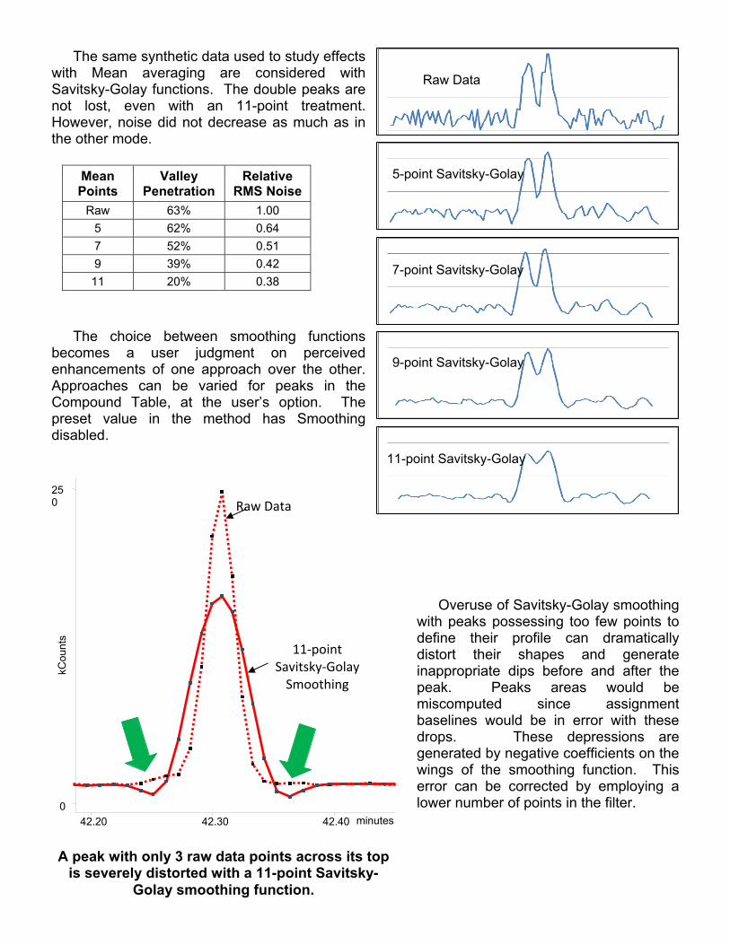
The same synthetic data used to study effects with Mean averaging are considered with Savitsky-Golay functions. The double peaks are not lost, even with an 11-point treatment. However, noise did not decrease as much as in the other mode.

The choice between smoothing functions becomes a user judgment on perceived enhancements of one approach over the other. Approaches can be varied for peaks in the Compound Table, at the user’s option. The preset value in the method has Smoothing disabled.

Overuse of Savitsky-Golay smoothing with peaks possessing too few points to define their profile can dramatically distort their shapes and generate inappropriate dips before and after the peak. Peaks areas would be miscomputed since assignment baselines would be in error with these drops. These depressions are generated by negative coefficients on the wings of the smoothing function. This error can be corrected by employing a lower number of points in the filter.

Mean Points

Valley Penetration

Relative RMS Noise

Raw 63% 1.00

5 62% 0.64

7 52% 0.51

9 39% 0.42

11 20% 0.38

Raw Data

5-point Savitsky-Golay




A peak with only 3 raw data points across its top is severely distorted with a 11-point Savitsky-

Golay smoothing function.

42.20 42.30 42.40 minutes0

250

kCou

nts

Raw Data

11‐point Savitsky‐Golay Smoothing

Treatment of Unknown Peaks All post-collection operations can be set for each compound individually, or parameters can be set to apply to all “Unknown Peaks”. Filtering, Integration Parameters and Timed Events can be selected to apply globally to all peaks not listed in the Compound Table. If “Report Unknown Peaks” is unchecked, then this “Chromatogram Processing” portion is grayed out and is not accessible. Potential Sources of Data Loss The amount of data involved in one measurement with a mass spectrometer is huge. The data set is a three-dimensional array of time, mass, and signal amplitude. Data transfer between spectrometer and computer is normally quite significant during the collection process. Every data point possesses a list of masses and intensities, and the transfer can occur at 12 Hz, or even faster with smaller mass ranges. The spectrometer can wait a bit for the computer to a reply to a hardware interrupt for the data transfer, but if the computer fails to react, possibly due to its doing many other tasks, some data points can be lost. When operations involve very fast data rates, then secondary operations with open Windows, especially actions involving accessing the hard drive, should be suspended until after the experiment is completed.

Many ant-virus software programs want to intercept all hard drive accesses, and look at the data stream before data can be written to the hard drive. This process can dramatically slow down data transfer from the spectrometer, and data can be lost. If possible, any anti-virus package on board should be set to ignore the VarianMS directory, or alternatively, to be disabled completely. A major impact of anti-virus programs is with .TMP files created by MS Workstation, and anti-virus programming needs to be set to disregard these as well.

Guidelines for Setting Optimum Parameters for Peak Detection

1. Collect data for a midrange standard with chromatography fully optimized. 2. Set Expected Peak Widths for each compound to match peak widths at ½ height

from the report for this midrange standard. 3. Set data rate and Scan Mode to enable at least 10 data points across top of the

narrowest peak in the chromatogram. 4. If sample peaks could have some low, noisy signals - say near their detection limits,

then set the Saviksky-Golay smoothing on with at least a 9-point smoothing function for all peak sizes.

5. Enable Spike Removal with a Spike Factor Threshold of 5. 6. Set Integration Windows wide enough to see “adequate” baseline before and after

each peak. 7. Set Identification Reference Peaks for compounds present in every sample,

typically Internal Standards and Surrogates. 8. Set Peak Reject Value just below lowest standard area counts. 9. Rerun or recalculate a midlevel standard to reset Expected Retention Time

windows.

10. Then SAVE method. 11. Run multi-level calibration sequence as required, with the last run being a mid-level

standard. 12. Reset Peak Reject Value to just below established detection limit and resave

method. 13. Run unknown samples.

This author thanks Ed Nygren, Dave Michelson and Dave Rhoades of Varian, Inc., for assistance in preparing this monograph.

Lotus Consulting 310/569-0128 Fax 714/898-7461 email [email protected]

5781 Campo WalkLong Beach, California 90803

Screens are copyrighted by Varian Inc., and are reprinted (reproduced) with the permission of Varian, Inc. All rights reserved.

Varian and the Varian logo are trademarks or registered trademarks of Varian, Inc. in the U.S. and other countries.

Peak Detection with Varian MS Workstation - Lotus...

Documents

Transcript of Peak Detection with Varian MS Workstation - Lotus...