TheRiskinHedgeFundStrategies: … TheoryandEvidencefrom TrendFollowers ... for an overview for hedge...

The Risk in Hedge Fund Strategies:Theory and Evidence fromTrend FollowersWilliam FungPI Asset Management, LLC

David A. HsiehDuke University

Hedge fund strategies typically generate option-like returns. Linear-factor models usingbenchmark asset indices have difficulty explaining them. Following the suggestions inGlosten and Jagannathan (1994), this article shows how to model hedge fund returns byfocusing on the popular “trend-following” strategy. We use lookback straddles to modeltrend-following strategies, and show that they can explain trend-following funds’ returnsbetter than standard asset indices. Though standard straddles lead to similar empiricalresults, lookback straddles are theoretically closer to the concept of trend following. Ourmodel should be useful in the design of performance benchmarks for trend-followingfunds.

The last decade has witnessed a growing interest in hedge funds frominvestors, academics, and regulators. Investors and academics are intriguedby the unconventional performance characteristics in hedge funds, and reg-ulators are concerned with the market impact of their reported speculativeactivities during major market events.1 The near bankruptcy of Long-TermCapital Management (LTCM) in 1998 has further heightened attention onhedge fund risk. Because hedge funds are typically organized as privateinvestment vehicles for wealthy individuals and institutional investors,2 theydo not disclose their activities publicly. Hence, little is known about the

This article received research support from the Foundation for Managed Derivatives Research and John W.Henry & Company. We acknowledge the New York Mercantile Exchange, the London International FinancialFutures Exchange, the Sydney Futures Exchange, and the Tokyo International Financial Futures Exchangefor providing their historical data; thanks to James Cui and Guy Ingram for computational assistance. Anearlier version benefited from comments by Todd Petzel, Jules Stanowicz, Richard Roll, Don Chance, DebraLucas, and the participants of the CBOT Winter Research Seminar on December 8–9, 1997, in Chicagoand the participants of the finance workshops at University of Washington at Seattle, Virginia PolytechnicInstitute, University of California at Los Angeles, the NBER Asset Pricing Program in Chicago (October30, 1998), University of Rochester, Washington University at St. Louis, and Carnegie-Mellon University.We are especially indebted to Joe Sweeney, Mark Rubinstein, and Ravi Jagannathan for valuable commentsand suggestions. Address correspondence to David A. Hsieh, Fuqua School of Business, Duke University,Box 90120, Durham, NC 27708-0120 or e-mail: [email protected].

1 See Fung and Hsieh (2000) and Fung et al. (1999) for analyses on the market impact of hedge fund activities.2 See Fung and Hsieh (1999) for an overview for hedge fund organizational structure and their economicrationale.

The Review of Financial Studies Summer 2001 Vol. 14, No. 2, pp. 313–341© 2001 The Society for Financial Studies

The Review of Financial Studies / v 14 n 2 2001

risk in hedge fund strategies. This article illustrates a general methodologyfor understanding hedge fund risk by modeling a particular trading strategycommonly referred to as “trend following” by the investment industry.As documented in Fung and Hsieh (1997a), hedge fund managers typi-

cally employ dynamic trading strategies that have option-like returns withapparently no systematic risk. Linear-factor models of investment styles usingstandard asset benchmarks, as in Sharpe (1992), are not designed to capturethe nonlinear return features commonly found among hedge funds. This maylead investors to conclude erroneously that there are no systematic risks.A remedy is in Glosten and Jagannathan (1994), where they suggested

using benchmark-style indices that have embedded option-like features.3 Thisis done in Fung and Hsieh (1997a) for hedge funds where they extracted stylefactors from a broad sample of hedge fund returns. By construction, thesestyle factors captured much of the option-like features while preserving thegeneral lack of correlation with standard asset benchmarks. To fully capturehedge fund risk, we must model the nonlinear relationships between thesestyle factors and the markets in which hedge funds trade. This is not a simpletask. The lack of public disclosure makes it difficult to link hedge fund stylefactors to asset markets.Our task is further complicated by the fact that hedge fund managers, who

are no strangers to risk, generally diversify their fund’s performance across avariety of strategies. Consequently, the observed returns and extracted stylefactors are generated by portfolios of different strategies, each having a dif-ferent type of risk. The combination of the dynamic allocation of capitalresources to a portfolio of trading strategies, each with nonlinear return char-acteristics, greatly limits the value of analyzing a general sample of manyhedge funds. From a modeling perspective, it is useful to concentrate on aspecific trading strategy that is identifiable with a reasonably large numberof hedge funds, whose returns are predominantly generated by that strategy.In this article, we focus on a popular strategy commonly referred to as

“trend following.”4 Trend following is a self-described strategy for the major-ity of commodity trading advisors (CTAs), as shown in Billingsley and

3 Typically, performance evaluation and attribution models rely on regressing a manager’s historical returns onone or more benchmarks. The slope coefficients reflect benchmark-related performance, whereas the constantterm (“alpha”) measures performance “benchmark risk.” This approach dates back to Jensen’s (1968) originalwork. Unfortunately, this type of regression method is sensitive to nonlinear relationships between the man-ager’s returns and the benchmarks and can result in incorrect inferences. For instance, Grinblatt and Titman(1989) showed that a manager can generate positive Jensen’s alphas by selling call options on the underlyingstocks of a given standard benchmark. Merton (1981) and Dybvig and Ross (1985) showed that a portfoliomanager with market-timing ability can switch between stocks and bonds to generate returns with option-likefeatures without explicitly trading options. Empirically, Lehman and Modest (1987) found that a number ofmutual funds exhibited option-like return features. A standard way to deal with option-like return featuresis to add nonlinear functions of the benchmark return as regressors. This was done in Treynor and Mazuy(1966) and Henriksson and Merton (1981).

4 Studies modeling other trading styles have emerged. See, for example, pairs trading in Gatev et al. (1999),risk arbitrage in Mitchell and Pulvino (1999), and relative-value trading in Richards (1999).

314

Risk in Hedge Fund Strategies

Chance (1996).5 Also, Fung and Hsieh (1997b) showed that the returns ofCTA funds have one dominant style factor. This implies that there is onedominant trading strategy in CTA funds, and that strategy is trend following.We therefore focus our empirical work on the return of CTA funds to developa model that explains their returns. In addition, this model contributes toexplaining the performance of other hedge funds that use trend following aspart of their portfolio of strategies.Trend following is a particularly interesting trading strategy. Not only

are returns of trend-following funds uncorrelated with the standard equity,bond, currency, and commodity indices, Fung and Hsieh (1997b) found thesereturns to exhibit option-like features—they tended to be large and positiveduring the best and worst performing months of the world equity markets.6

This is evident in Exhibit 2 of Fung and Hsieh (1997b), reproduced hereas Figure 1. The monthly returns of the world equity market, as proxied bythe Morgan Stanley (MS) World Equity Index, are sorted into five “states.”State 1 consists of the worst months, and State 5 the best months. This figuregraphs the average monthly return of an equally weighted portfolio of the sixlargest trend-following funds, along with that of the world equity markets, ineach state. Fung and Hsieh (1997b) noted that a similar pattern holds for anequally weighted portfolio of all trend-following funds.The return profile shown in Figure 1 indicates that the relationship

between trend followers and the equity market is nonlinear. Although returnsof trend-following funds have a low beta against equities on average, thestate-dependent beta estimates tend to be positive in up markets and nega-tive in down markets. In fact, the return pattern of trend-following funds inFigure 1 is similar to those of contingent claims on the underlying asset andmust therefore have systematic risk, albeit in a nonlinear manner. The goalof this article is to model how trend followers achieve this unusual returncharacteristic in order to provide a framework for assessing the systematicrisk of their strategy. Note that, in the presence of nonlinearity, betas froma standard linear-factor model can either overstate the systematic risk orunderstate it (as in the case of LTCM).If the trading rules used by trend followers are readily available, we can

directly estimate their systematic risk. Unfortunately, but understandably,traders regard their trading systems to be proprietary and are reluctant todisclose them. We can therefore only theorize what trend followers do. Fur-thermore, although we use the term trend followers to describe a certain class

5 CTAs are individuals or trading organizations, registered with the Commodity Futures Trading Commission(CFTC) through membership in the National Futures Association, who trade primarily futures contracts onbehalf of a customer.

6 August 1998 provides an out-of-sample observation that substantiates this view. While the S&P 500 lost14.5% of its value, commodity funds generally had positive returns. In a Barron’s September 9, 1998, article,Jaye Scholl wrote, “Of the 17 commodity trading advisors reporting to MAR, 82% generated positive resultsin August, with 46 of them posting returns of more than 10%.”

315


Figure 1Average monthly returns of six large trend-following funds in five different MS world equity marketstatesSource: Fung and Hsieh (1997a).

of traders, in practice their respective approaches can differ widely. Trendfollowers can converge onto the same “trend” for different reasons and havevery different “entry and exit” points. From a modeling perspective, we needa level of aggregation that captures the essence of this trading style but avoidssome of the distracting idiosyncrasies of individual trend followers.We posit that the simplest trend-following strategy, which we label as

the “primitive trend-following strategy,” has the same payout as a structuredoption known as the “lookback straddle.” The owner of a lookback call optionhas the right to buy the underlying asset at the lowest price over the life ofthe option. Similarly, a lookback put option allows the owner to sell at thehighest price. The combination of these two options is the lookback straddle,which delivers the ex post maximum payout of any trend-following strategy.7

The concept of a lookback option was first introduced in Goldman et al.(1979). Within this context, trend followers should deliver returns resemblingthose of a portfolio of bills and lookback straddles. Unlike earlier studies that

7 In reality, trend followers often make multiple entry and exit decisions over a sufficiently long investmenthorizon so long as there is sufficient volatility surrounding the underlying trend. This aspect is excluded inour simple model. However, a comparison of our model to the market-timing model of Merton (1981) can befound in Section 2 of this article.

316


explicitly specify “technical trading rules” to proxy a popular form of trend-following strategy,8 this particular option strategy is not designed to replicateany specific trend-following strategy. Rather, it is designed to capture thegeneral characteristics of the entire family of trend-following strategies.We demonstrate empirically that lookback straddle returns resemble the

returns of trend-following funds. This provides the key link between thereturns of trend-following funds and standard asset markets.The rest of the article is organized as follows. Section 1 sets out the theoret-

ical foundation of the primitive trend-following strategies as lookback strad-dles. We explore the similarities and differences between trend following andmarket timing as trading strategies in the Merton (1981) framework. Givenany asset, we show that the lookback straddle is better suited to capture theessence of trend-following strategies than a simple straddle. Section 2 detailsthe data sample used to test our model. Section 3 reports the improvementson explaining trend-following funds’ returns using our model versus standardasset benchmarks. It confirms the intuition that trend-following funds’ returnsare similar to those of contingent claims on standard asset indices. Section 4discusses the question of performance benchmarks for trend followers. Herewe note the opportunistic nature of trend followers. These traders apply capi-tal resources to different markets in a dynamic fashion and do so in a mannerpeculiar to their individual skill and technology. Summary and conclusionsare in Section 5.

1. The Primitive Trend-Following Strategy

The convex return pattern observed in Figure 1 resembles the payout profileof a straddle on the underlying asset. A simple strategy that yields the returnpattern of a straddle is that of a “market timer” who can go long and shorton the underlying asset, as in Merton (1981). Following his notation, let Z(t)

denote the return per dollar invested in the stock market and R(t) the returnper dollar invested in Treasury bills in period t . At the start of the period,if the market timer forecasts stocks to outperform bills, only stocks will beheld. Otherwise, only bills will be held. This implicitly assumes the presenceof short sales constraints. For a perfect market timer, Merton (1981) showedthat the return of his portfolio is given by R(t)+Max{0, Z(t)−R(t)}, whichis the return of a portfolio of bills and a call option on stocks.In the absence of short sale constraints, the market timer’s return

is modified to reflect the short sale alternative. For a perfect markettimer, Merton (1981) showed that the return of his portfolio is given byR(t)+Max{0, Z(t)−R(t)}+Max{0, R(t)−Z(t)}, which is the return of aportfolio of bills and a straddle on stocks. In a follow-up paper, Henriksson

8 See Alexander (1961).

317


and Merton (1981) proposed a nonparametric test on whether a market timerhad the ability to time the market.We use a similar approach to model a trend follower. It is helpful to

begin with a qualitative comparison of market timing and trend following astrading strategies. Both market timers and trend followers attempt to profitfrom price movements, but they do so in different ways. In Merton (1981),a market timer forecasts the direction of an asset, going long to capture aprice increase, and going short to capture a price decrease. A trend followerattempts to capture “market trends.” Trends are commonly related to serialcorrelation in price changes, a concept featured prominently in the early testsof market efficiency. A trend is a series of asset prices that move persistentlyin one direction over a given time interval, where price changes exhibit posi-tive serial correlation. A trend follower attempts to identify developing pricepatterns with this property and trade in the direction of the trend if and whenthis occurs.9

To provide a formal definition of these two trading strategies, we intro-duce the concepts of Primitive Market-Timing Strategy (PMTS) and Primi-tive Trend-Following Strategy (PTFS) as follows. Let S, S ′, Smax , and Smin

represent the initial asset price, the ending price, the maximum price, andthe minimum price achieved over a given time interval. Consistent with theMerton (1981) framework, we restrict our strategies to complete a singletrade over the given time interval. The standard buy-and-hold strategy buys atthe beginning and sells at the end of the period, generating the payout S ′ −S.The PMTS attempts to capture the price movement between S and S ′. If S ′

is expected to be higher (lower) than S, a long (short) position is initiated.The trade is reversed at the end of the period. Thus, the optimal payout ofthe PMTS is |S ′ − S|. The PTFS, on the other hand, attempts to capture thelargest price movement during the time interval. Consequently, the optimalpayout of the PTFS is Smax − Smin. Note that the PMTS is defined in a man-ner consistent with Merton (1981). The construction of the PTFS, on otherhand, adds the possibility of trading on Smax and Smin.

10 Capital allocation tothe PMTS or PTFS is determined by comparing the payout of the respectivestrategy to the return of the risk-free asset.11

If we are dealing with perfect market timers and perfect trend followers,they would capture the optimal payouts |S ′ −S| and Smax −Smin, respectively,without incurring any costs. In reality, these traders cannot perfectly antic-ipate price movements. A helpful distinction between their approaches canbe made as follows. Generally, market timers enter into a trade in anticipa-tion of a price move over a given time period, whereas trend followers trade

9 Note that we are not advocating that markets trend. That is an empirical issue best deferred to another occasion.10 Therefore, if Merton’s (1981) assumptions were strictly imposed, the payout of the PTFS must equal that ofthe PMTS.

11 The distribution of capital resources between the respective trading strategy and the riskless asset will alsodepend on the investor’s risk preference.

318


only after they have observed certain price movements during a period. Theterms buying breakouts and selling breakdowns are often used to describetrend followers.12 These are very common characteristics of trend-followingstrategies.Also, in reality, market timers and trend followers do incur costs when

they attempt to capture their respective optimal payouts. We cannot estimatethese costs without knowledge of their strategies. Instead, we assume that theex ante cost of the PMTS is the value of an at-the-money standard straddle,and that of the PTFS is the value of a lookback straddle. In other words,the PMTS is a long position in a standard straddle, and the PTFS is a longposition in a lookback straddle.In the next section, we will empirically create returns of the PTFS using

lookback straddles on 26 different markets. Before doing so, we have someremarks regarding the differences between the PTFS and the PMTS.As the PMTS and PTFS are option positions, we can illustrate their theo-

retical difference via their deltas. For illustrative purposes, assume that Blackand Scholes (1973) holds. The price of a standard straddle is then wellknown, and the prices of lookback options can be found in Goldman et al.(1979). The delta of the standard straddle is given by

δ = 2N(a1) − 1, (1)

where N( ) is the cumulative standard normal distribution, and

a1 = [ln(S/X) + (r + 1

2σ2)T ]/(σT 1/2). (2)

Here, S is the current price of the underlying asset with instantaneous vari-ance σ, r the instantaneous interest rate, and T the time to maturity of theoption. In comparison, the delta of the lookback straddle is given by

δLB = [1 + 12σ

2/r] N(−b3) + (u/σ) exp(−rT + 2rb/σ 2) N(b2)

− [1 + 12σ

2/r] N(d3) − (u/σ) exp(−rT − 2rd/σ 2) N(d2), (3)

where

u = (r − 12σ

2), (4)

d = ln(S/Q) (5)

d1 = [ln(S/Q) + (r − 12σ

2)T ]/(σT 1/2), (6)

d2 = [− ln(S/Q) + (r − 12σ

2)T ]/(σT 1/2), (7)

d3 = [− ln(S/Q) − (r + 12σ

2)T ]/(σT 1/2), (8)

12 Breakout means that the price of an asset moves above a recent high, and buying breakouts refers to thestrategy of going long when a breakout happens. Breakdown means that the price moves below a recent low,and selling breakdowns refers to the strategy of going short when a breakdown happens.

319


b = ln(M/S), (9)

b1 = [ln(M/S) − (r − 12σ

2)T ]/(σT 1/2), (10)

b2 = [− ln(M/S) − (r − 12σ

2)T ]/(σT 1/2), and (11)

b3 = [ln(M/S) − (r + 12σ

2)T ]/(σT 1/2). (12)

Here Q and M denote the minimum and maximum prices, respectively,of the asset since the inception of the lookback straddle. A derivation ofEquation (3) is available from the authors on request. Several examples ofthe difference in the deltas are in Appendix A. The key difference lies in thepath-dependency of the lookback option.Empirically, the difference between the PMTS and the PTFS is much more

subtle. Given any investment horizon, the payout of the PMTS equals thatof the PTFS if and only if Smax and Smin occur at the beginning and end ofthe period in any order. Consequently, as the investment horizon shrinks, thepayouts of the two strategies converge. As the investment horizon lengthens,the payout of the two strategies will diverge, because the probability of Smax

and Smin being interior points to the investment horizon increases. In theempirical implementation, we use three-month options, which tend to bethe most liquid options; this observation period may be too short to delivera consistently dramatic payout difference between lookback straddles andstandard straddles.Furthermore, as pointed out in Goldman et al. (1979), the lookback straddle

can be replicated by dynamically rolling standard straddles over the life of theoption. The rollover process is much reminiscent of the buying breakouts andselling breakdowns characteristics of trend-following strategies.13 However,as both the PMTS and PTFS make use of standard straddles on the sameasset, albeit in a different manner, their returns are likely to be correlated.Given these two considerations, it may be difficult to distinguish between

the PMTS and the PTFS empirically, even though the PTFS better describestrend-following strategies theoretically. This issue is explored in the empiri-cal sections of the article. We note here that the goal of this article is to showthat there is at least one option portfolio, involving bills and lookback strad-dles, that performs like trend-following funds. We do not attempt to answerthe question of which option portfolio best describes the returns of trend-following funds. It is conceivable that, depending on the data sample used,alternative strategies to the PTFS can better replicate trend-following funds’returns empirically.

13 A more detailed description of this process can be found in Section 3.

320


2. Constructing a Performance Database of PTFSs

To verify if the PTFS can mimic the performance of trend followers, wegenerated the historical returns of the PTFS applied to the most active mar-kets in the world. For stock indices, we used the futures contracts on theS&P 500 (CME), Nikkei 225 (Osaka), FTSE 100 (LIFFE), DAX 30 (DTB),and the Australian All Ordinary Index (SFE). For bonds, we used the futurescontracts on the U.S. 30-year Treasury bonds (CBOT), UK Gilts (LIFFE),German Bunds (LIFFE), the French 10-year Government Bond (MATIF),and the Australian 10-year Government Bond (SFE). For currencies, weused the futures contracts on the British pound, Deutschemark, Japaneseyen, and Swiss franc on the CME. For three-month interest rates, we usedthe futures contracts on the 3-month Eurodollar (CME), Euro-DeutscheMark (LIFFE), Euro-Yen (TIFFE), the Paris Interbank Offer Rate (PIBOR)(MATIF), 3-month Sterling (LIFFE), and the Australian Bankers AcceptanceRate (SFE). For commodities, we used the futures contracts on soybean,wheat, and corn futures traded on the CBOT and gold, silver, and crude oiltraded on the NYMEX.Futures and option data on the DTB, MATIF, and Osaka were purchased

from the Futures Industry Institute (FII). Futures and option data on theLIFFE, SFE, and TIFFE and option data on the CBOT and NYMEX weresupplied by the respective exchanges. Option data on the CME were pur-chased from the FII and updated by the CME. Futures data on the CBOT,CME, and NYMEX came from Datastream. Appendix B provides informa-tion on the data.A number of technical complications arose in the construction of the PTFS

returns. First, lookback options are not exchange-traded contracts, so we can-not directly observe their prices. Instead, we replicated the payout of a look-back straddle by rolling a pair of standard straddles, as described in Goldmanet al. (1979). The replication process calls for the purchase of two at-the-money straddles at inception using standard puts and calls. We use one strad-dle to lock in the high price of the underlying asset by rolling this straddle toa higher strike whenever the price of the underlying asset moves above thecurrent strike. At expiration, this straddle’s strike must equal the highest priceachieved by the underlying asset since inception. We use the other straddleto lock in the lowest price of the underlying asset by rolling the straddle toa lower strike whenever the price of the underlying asset moves below thecurrent strike. At expiration, this latter straddle’s strike must equal the lowprice achieved by the underlying asset since inception. Thus, the pair of stan-dard straddles must pay the difference between the maximum and minimumprice achieved by the underlying asset from inception to expiration, which isexactly the payout of the lookback straddle.14

14 An alternative replication strategy is a delta-hedging strategy using the underlying asset. However, a delta-hedging strategy has two problems. First, we need the implied volatility of the option to calculate its delta.

321


Second, though the strategy of rolling standard straddles can replicate thepayout of the lookback straddle, it may not perfectly replicate all the cashflows of the lookback straddle. A lookback straddle has only two cash flows:an upfront premium at inception and a payout equal to the maximum rangeof the price of the underlying asset at expiration. In replicating this, thestraddle rolls may generate additional cash flows when straddles are rolledfrom one strike price to another. We included these cash flows in calculatingthe returns of the straddle-rolling strategy.Third, our straddle-rolling strategy ignores the fact that many exchange-

traded options are not European-style options. Most of the options traded onU.S. exchanges are American-style options, which have higher prices thanEuropean-style options. This biases downward the returns of the PTFS. Thereis no problem with options on the LIFFE, which are futures-style options.Fourth, we frequently do not observe at-the-money options. Because

exchange-traded options have discrete strikes, we use the nearest-to-the-money options to approximate at-the-money options. The error is likely tobe small.Fifth, we have to select the horizon of the lookback straddle. The choice is

primarily dictated by availability and liquidity of the options in our data set.All the financial options in our data set have quarterly expirations. Even whenmonthly expirations are available, quarterly expirations tend to have longerhistory and larger volume. In the case of commodity options, the majorityhave expirations in March, June, September, and December. To compareresults across markets, we used lookback straddles with three months toexpiration as close to the end of a quarter as possible to maintain consistency.Finally, the straddle-rolling strategy should be implemented continuously

if we were to match the assumptions in Goldman et al. (1979) exactly. Thisis impractical, as it requires tick-by-tick data, which are costly to purchaseand time-consuming to process. It is also unclear to what extent it is feasibleto simulate straddle rolls on a tick-by-tick basis, due to the asynchronousnature of options trading (at different strikes) and the potential distortion ofbid-offer spreads. In practice, we rolled the straddles only at the end of eachtrading day using the settlement prices of the options and the underlyingassets. We then aggregated the daily returns up to monthly returns to matchthe standard reporting interval for hedge funds.The monthly returns of the PTFS from rolling the straddles are summa-

rized in Table 1. Based on these return series, we formed five portfolios ofstraddles, one each for stocks, bonds, three-month interest rates, currencies,and commodities. Their correlation matrix is given in panel G of Table 1.

As lookback options are not traded, we will have to make some assumptions to obtain an implied volatility.Second, a delta-hedging strategy can incur substantial transaction costs, as it requires dynamically changingthe amount of the underlying asset every time its price changes. The straddle-rolling strategy will incur manyfewer transactions.

322


Table 1Statistical properties of primitive trend-following strategy (PTFS) returns for 26 markets and5 portfolios

Panel A: PTFS monthly returns for stock markets

S&P FTSE DAX Nikkei Australian500 100 30 225 All Ordinary

Mean −0.0161 −0.0177 0.0437c −0.0470 −0.0304c

SD 0.2774 0.1845 0.2775 0.3978 0.1627Maximum 2.2932 0.5313 1.0060 1.7349 0.3912Minimum −0.4003 −0.3867 −0.3433 −0.7667 −0.2657Skewness 3.83a 0.71a 1.19a 1.72a 0.88a

% positive 33 41 44 33 32

Panel B: PTFS monthly returns for government bond markets

US UK German French Australian30Y Gilt Bund 10Y 10Y

Mean 0.0136 0.0097 0.0321c 0.0157 0.0189SD 0.2455 0.2351 0.2333 0.2285 0.2411Maximum 0.9642 0.8859 1.2051 0.9989 0.6884Minimum −0.3503 −0.3110 −0.3117 −0.4464 −0.3881Skewness 1.55a 1.21a 2.16a 1.43a 0.93a

% positive 40 40 49 49 39

Panel C: PTFS monthly returns for three-month interest rate markets

Australia Paris3-month Bankers Interbank

Euro-Dollar Sterling Euro-DM Euro-Yen Acceptance Rate

Mean 0.0170 0.0449c −0.0375 0.0750c 0.0453 0.0513c

SD 0.2703 0.3495 0.3077 0.4066 0.4780 0.3167Maximum 1.0174 1.4412 1.8883 2.2039 2.4999 1.5699Minimum −0.5000 −0.4129 −0.4444 −0.4545 −0.4950 −0.4433Skewness 1.33a 1.59a 3.20a 2.38a 2.72a 1.70a

% positive 40 39 31 45 36 50

Panel D: PTFS monthly returns for currency markets

British Pound Deutsche Mark Japanese Yen Swiss Franc

Mean 0.0174 0.0232 0.0455c 0.0496a

SD 0.3070 0.2788 0.3372 0.2577Maximum 1.2661 1.0783 1.3560 1.1054Minimum −0.4391 −0.3992 −0.4223 −0.3513Skewness 1.73a 1.48a 1.67a 0.99a

% positive 41 38 44 48

Panel E: PTFS monthly returns for commodity markets

Corn Wheat Soybean Crude Oil Gold Silver

Mean −0.0135 0.0435c −0.0355c 0.0455b −0.0539a −0.0502b

SD 0.2685 0.2977 0.3001 0.3047 0.2927 0.2685Maximum 1.5408 1.3286 1.1063 2.1573 1.0266 1.0952Minimum −0.4286 −0.3914 −0.5556 −0.3716 −0.5119 −0.4982Skewness 1.87a 1.74a 1.54a 2.93a 1.37a 1.52a

% positive 37 45 33 44 30 33

Before proceeding to compare the PTFS returns to trend-following funds’returns, we examine the empirical difference between the standard straddleand the lookback straddle. We start by comparing the two types of straddleson two quarterly options on the Japanese yen futures contract.

323


Table 1(continued)

Panel F: Monthly returns for trend followers and five PTFS portfolios (1989–97)

Trend-Following Stock Bond Interest Currency CommodityFunds PTFS PTFS Rate PTFS PTFS PTFS

Mean 0.0137a −0.0193 0.0181 0.0195 0.0177 −0.0072SD 0.0491 0.2094 0.1573 0.1867 0.2305 0.1310Maximum 0.1837 1.3240 0.4739 0.8158 1.0006 0.6413Minimum −0.0820 −0.5172 −0.2285 −0.2573 −0.3013 −0.2497Skewness 0.79a 2.62a 1.07a 1.46a 1.68a 1.19a

Panel G: Correlation matrix of the five PTFS portfolios

Stock Bond Interest Currency CommodityPTFS PTFS Rate PTFS PTFS PTFS

Stock PTFS 1.00 0.37 0.06 0.16 0.37Bond PTFS 1.00 0.32 0.21 0.12Interest rate PTFS 1.00 0.36 0.07Currency PTFS 1.00 0.18Commodity PTFS 1.00

The primitive trend-following strategy (PTFS) is a long position on three-month lookback straddles. The five PTFS portfoliosare equally weighted portfolios of the PTFSs in the five groups of markets (panels A through E). Trend-following funds’ returnsare based on an equally weighted portfolio of 407 defunct and operating commodity funds that had significant correlation withthe first principal component from a principal component analysis of 1304 defunct and operating commodity funds. The sampleperiods for each market is given in Appendix B.aStatistically different from zero at the 1% one-tailed test.bStatistically different from zero at the 5% one-tailed test.cStatistically different from zero at the 10% one-tailed test.%Positive refers to the percentage of months with positive returns.

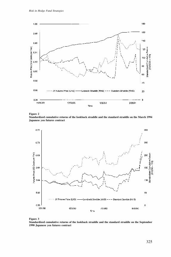
The first comparison is graphed in Figure 2, using the March 1994Japanese yen contract. We initiated the straddles at the end of November1993, approximately three months prior to expiration. At that time, the Marchyen futures price was 0.9199. It declined to a low of 0.8878 in early January1994, rose to a high of 0.9780 by mid-February, and ended at 0.9459 whenthe contract expired in the middle of March. As the contract’s minimumand maximum prices occurred in the middle of the observation period, thepayout of the lookback straddle (0.0902) was substantially greater than thatof the standard straddle (0.0260).The second comparison is graphed in Figure 3, using the September 1990

Japanese yen futures contract. Like the first comparison, we initiated thestraddles at the end of May 1990, approximately three months prior toexpiration. At that time, the September yen futures price was 0.6591. Itdeclined to a low of 0.6444 near the end of June, and then rose to a highof 0.7147 at the expiration of the contract. In this case, the contract’s min-imum and maximum prices occurred near the beginning and the end of theobservation period, so the payout of the lookback straddle (0.0703) wasmuch closer to that of the standard straddle (0.0556). These two graphsshow that the two straddles can have different payouts over a given obser-

324


Figure 2Standardized cumulative returns of the lookback straddle and the standard straddle on the March 1994Japanese yen futures contract

Figure 3Standardized cumulative returns of the lookback straddle and the standard straddle on the September1990 Japanese yen futures contract

325


vation period, depending on when the maximum and minimum prices werereached.Next, we examine the entire data sample from March 1986 to December

1997. The daily returns of the two types of straddles on the Japanese yenhad a correlation of 0.39, and their monthly returns had a correlation of 0.86.This indicates that, in our empirical application using monthly returns, thedifference between the PMTS and the PTFS may be hard to discern. Thisis a consequence of using monthly returns of options that expire quarterly.We are empirically constrained to use quarterly options because data forlonger-dated options are generally unreliable and, in most cases, unavailable.In addition, we are also empirically constrained to use monthly returns ashigher frequency observations on the performance of trend-following fundsare limited. It is an empirical regularity that the standard straddle and thelookback straddle are highly correlated in our data sample, even though thisis not necessarily so at a different return interval. Consequently, we applythe lookback straddle in our empirical tests given its superior theoreticalproperties.

3. Evaluating the Risk in Trend-Following Strategies

In this section we show that the returns of trend-following funds are stronglycorrelated with the returns of the PTFSs. This is consistent with the notionthat trend-following funds have systematic risks, contrary to the predictionof linear-factor models applied to standard asset benchmarks.

3.1 Standard benchmarks do not explain trend-following funds’ returnsTo explore this issue, we begin with a representative series of trend-followingfunds’ returns. Theoretically, different trend-following funds may use differ-ent trading strategies. This may require a tailor-made benchmark for eachfund, based on extensive interviews with the manager. Fortunately, despite thetheoretical differences in the strategies, there is a high degree of commonalityin the returns of trend-following funds, as shown in Fung and Hsieh (1997b).Applying principal components analysis on all defunct and operating CTAfunds, Fung and Hsieh (1997b) found a single dominant trading style. Thisdominant style was interpreted to be a trend-following style, which is themost popular self-described CTA trading style. In this article, we update theresults of Fung and Hsieh (1997b) using the Tass CTA database as of March1998. Out of 1304 defunct and operating CTA funds, 407 are strongly corre-lated to the first principal component.15 The returns of the equally weighted

15 Fung and Hsieh (1997b) noted that the inclusion of defunct funds helps guard against “survivorship bias” intheir estimate of the returns of the trend-following trading style. Survivorship bias comes about when onlysurviving, or operating, funds are used to estimate the returns of a group of funds. This is likely to result inan upward bias, because the omitted defunct funds generally have poorer performance than surviving funds.

326


portfolio of these 407 funds are used as the representative trend-followingfunds’ returns.We start with a key distributional feature of trend-following funds’ returns.

Table 1 shows that the trend-following funds’ returns have strongly posi-tively skewed returns. The returns of the five PTFS portfolios as well as allthe individual PTFSs are also strongly positively skewed. The difference isthat trend-following funds’ returns have a positive and statistically significantmean, whereas the PTFS portfolios and most of the individual PTFSs do not.With the exception of the PTFS for the Swiss franc, trend-following funds’returns have a higher mean and greater statistical significance than the PTFSreturns. We defer further analysis of this implicit alpha in trend-followingfunds’ returns until Section 4.

3.2 Lookback straddle benchmarks explain trend-following funds’returns

Next, we document the apparent lack of systematic risk in trend-followingfunds’ returns in standard linear-factor models in Table 2. The regres-sion of trend-following funds’ returns against the eight major asset classes

Table 2Explaining trend-following funds’ returns: The �R2s of regressions on ten sets of risk factors

Sets of Risk Factors �R 2 of Regression (%)

1. Eight major asset classes in Fung and Hsieh (1997a) 1.0(U.S. equities, non-U.S. equities, U.S. bonds, non-U.S. bonds,gold, U.S. dollar index, Emerging market equities,one-month Eurodollar)

2. Five major stock indices −2.1(S&P 500, FTSE 100, DAX 30, Nikkei 225, AustralianAll Ordinary)

3. Five government bond markets 7.5(U.S. 30-year, UK Gilt, German Bund,French 10-year, Australian 10-year)

4. Six three-month interest rate markets 1.5(Eurodollar, 3m Sterling, Euro-DM, Euro-Yen,Australian Bankers Acceptance,Paris Interbank Rate)

5. Four currency markets −1.1(British pound, deutschemark, Japanese yen,Swiss franc)

6. Six commodity markets −3.2(corn, wheat, soybean, crude oil, gold, silver)

7. Goldman Sachs Commodity Index −0.7

8. Commodity Research Bureau Index −0.8

9. Mount Lucas/BARRA Trend-Following Index 7.5

10. Five PTFS portfolios 47.9(Stock PTFS, Bond PTFS, Currency PTFS,three-month interest rate PTFS, Commodity PTFS)

�R 2 refers to adjusted R2 of the regressions of trend-following funds’ returns on ten different sets of risk factors.

327


(U.S. equities, non-U.S. equities, U.S. bonds, non-U.S. bonds, one-monthEurodollar interest rate, gold, U.S. Dollar Index, and emerging marketequities) in Fung and Hsieh (1997a) has an �R2 of 1.0%, and none of thevariables are statistically significant. For completeness, we examined the26 markets used to construct the PTFSs in Table 1. Doing this by groups,the five stock markets have an �R2 of −2.1%, the five bond markets 7.5%,the six three-month interest rates 1.5%, the four currencies −1.1%, and thesix commodities −3.2%. An investor using a linear-factor model on stan-dard asset benchmarks would have concluded that trend followers had nosystematic risk.Other indices frequently associated with commodity traders and trend fol-

lowers produced similarly poor results. The regression of trend-followingfunds’ returns on the GSCI Total Return Index has an �R2 of −0.7% and isnot statistically significant. The Commodity Research Bureau (CRB) Indexhas an �R2 of −0.8% and is also not significant. The Mount Lucas/BARRATrend-Following Index is slightly better, with an �R2 of 7.5%, and it is sta-tistically significant. These results are summarized in Table 2.Next, we document the PTFS’s ability to characterize the performance of

trend followers using standard linear statistical techniques. The regression ofthe trend-following funds’ returns on the five PTFS portfolios returns has an�R2 of 47.9%, with currencies and commodities having the largest explanatorypower. The F -test that none of the PTFS portfolios is correlated with thetrend-following funds’ returns is rejected at any conventional significancelevel. This indicates that trend followers do have systematic risks. Theserisks are just not evident in a linear-factor model applied to standard assetbenchmarks.Proper diagnostics are needed to guard against nonlinear relationships in

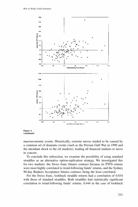
regressions. We do so using scatter plots of the trend-following funds’ returnsagainst the five PTFS portfolios in the five panels in Figure 4. The first panelgraphs the trend-following funds’ returns against the stock PTFS returns.It basically shows that there is no apparent relationship between these twovariables either in the center of the distribution or at the extremes. The otherpanels in Figure 4 are the scatter plots of the trend-following funds’ returnsagainst the PTFS portfolios in bonds, three-month interest rates, currencies,and commodities, respectively. They show that the currency and commodityPTFSs have the strongest relationship with trend followers. In particular, thepanel for currency PTFS contains the most striking scatter plot. It shows that,when trend followers make large profits, the currency PTFS also makes largeprofits. In fact, the relationship between the currency PTFS returns and thetrend-following funds’ returns appear reasonably linear. Plots of the residualsof the regression against the explanatory variables (available from the authorson request) do not show any remaining nonlinear relationships.

328


3.3 Trend-following funds’ returns are sensitive to large moves in worldequity markets

Next we examine another important characteristic of trend-following funds’returns corresponding to extreme moves in world equity markets. We beginwith Table 3, where we report the trend followers’ sizable positive returnsduring downturns in world equity markets. The two worst periods for worldequities in the last 10 years, as measured by the MS World Equity index,are: Sep–Nov 1987 (−20.4%) and Aug–Sep 1990 (−18.9%). Trend-followingfunds recorded large positive returns of 13.0% and 10.2% during these twoperiods, respectively. Given the lookback option’s structure, it was not sur-prising that the PTFSs for stocks had positive returns during these two downperiods for equities. The less obvious results were the positive returns fromthe PTFSs for most of the government bonds, currencies, and commodities.However, less than half of the PTFSs for three-month interest rates wereprofitable during these two periods.To generalize these unusual return characteristics, we provide further col-

laborating evidence on this relationship between the returns of trend followersand those of the world equity markets over a large sample period. It was firstobserved in Fung and Hsieh (1997a, 1997b) that the returns of trend follow-ers have option-like payouts relative to world equity markets. We extend thisobservation to encompass a larger data set using the returns from the PTFSs.The result is reported in Table 4. Here we divided the longer time series forwhich there were data for all PTFSs (March 1985 to December 1997) into5 states, based on the performance of the world equity market. State 1 rep-resents the worst 30 months for world equities, which declined on average4.60%. State 2 consists of the next 30 worst months, when equities fell anaverage of 0.59% per month. State 5 has the best 30 months for equities,which rose 6.74% on average. State 4 are the next best 30 months, in whichequities gained 3.36% on average. State 3 contains the remaining 34 months.We then report the average return and the standard deviation of the PTFSsfor stocks, bonds, currencies, three-month interest rates, and commoditiesduring these states.Consistent with the earlier observation, the returns of the PTFSs tended to

be high during extreme states 1 and 5 for stocks. As expected, the PTFSs onstocks had high and positive average returns during the two extreme states.The PTFSs on bonds, three-month interest rates, and currencies also hadhigh and positive average returns in states 1 and 5. However, the PTFSs oncommodities did not exhibit this option-like behavior.16

It is perhaps not surprising that the PTFSs in bonds, three-month inter-est rates, and currencies generated high returns during extreme moves in theworld equity markets. Theoretically, financial assets (stocks, bonds, three-month interest rates, and currencies) should respond to the same set of

16 The low average return for the commodity PTFS in state 1 was primarily due to one outlier.

329


Figure 4Scatter plots of monthly trend-following funds’ returns versus five PTFS portfolio returns

330


Figure 4(continued)

macroeconomic events. Historically, extreme moves tended to be caused bya common set of dramatic events (such as the Persian Gulf War in 1990 andthe attendant shock to the oil markets), leading all financial markets to movein concert.To conclude this subsection, we examine the possibility of using standard

straddles as an alternative option-replication strategy. We investigated thisfor two markets: the Swiss franc futures contract because its PTFS returnswere most highly correlated to trend-following funds’ returns, and the Sydney90-day Bankers Acceptance futures contract, being the least correlated.For the Swiss franc, lookback straddle returns had a correlation of 0.834

with those of standard straddles. Both straddles had statistically significantcorrelation to trend-following funds’ returns, 0.444 in the case of lookback

331


Table 3Large PTFS returns during the two worst periods for world equities: Sep–Nov 1987 and Aug–Sep 1990

Panel A: World equities and trend-following funds

MS World Trend-FollowingPeriod Equities Funds

8709–8711 −0.2036 0.12999008–9009 −0.1889 0.1019

Panel B: PTFS returns for stock markets

Stock Australian AllPeriod PTFS S&P 500 FTSE 100 DAX 30 Nikkei 225 Ordinary

8709–8711 2.1060 2.10609008–9009 0.7744 0.7744

Panel C: PTFS returns for bond markets

Period Bond PTFS US 30Y UK Gilt German Bund French 10Y Australian 10Y

8709–8711 0.2725 0.3187 0.07539008–9009 0.3557 0.3670 −0.0513 0.1257 1.0377

Panel D: PTFS returns for three-month interest rate markets

Australia ParisInterest Bankers Interbank

Period Rate PTFS Euro-Dollar 3-month Sterling Euro-DM Euro-Yen Acceptance Rates

8709–8711 0.8194 0.81949008–9009 −0.1372 −0.0052 −0.0898 −0.3145 0.4268

Panel E: PTFS returns for currency markets

Period Currency PTFS British Pound Deutsche Dark Japanese Yen Swiss Franc

8709–8711 0.7758 1.3368 0.5401 0.3842 0.74489008–9009 0.1832 0.1887 −0.0599 0.0882 0.5165

Panel F: PTFS returns for commodity markets

Period Commodity PTFS Corn Wheat Soybean Crude Oil Gold Silver

8709–8711 0.0220 0.1494 0.8344 −0.3871 −0.39379008–9009 0.8525 0.4336 0.2040 −0.2891 5.4406 0.9578 0.1719

straddles and 0.433 for standard straddles. For the Sydney 90-day BankersAcceptance, lookback straddle returns had a correlation of 0.924 with thoseof standard straddles. Neither straddle, however, had statistically significantcorrelation with trend-following funds’ returns, −.006 in the case of look-back straddles and 0.010 in the case of standard straddles. These resultsindicate that, for quarterly expirations, standard straddles are similar to look-back straddles for the purpose of replicating monthly trend-following funds’returns. Our choice of the lookback straddle in the empirical application restson its superior theoretical properties given in Section 2.

3.4 Preferred habitat of trend followersNext we address the question of preferred habitat or which markets trendfollowers were active in during the extreme equity market moves (i.e., states1 and 5 in Table 4). To answer this question, we regressed the trend-followingfunds’ returns on the PTFSs’ returns during the extreme states 1 and 5. Given

332


Table 4Option-like behavior of PTFS returns during five different states for equities: Mar 85–Dec 97

Interest Commodity Trend Following MS WorldState Stock PTFS Bond PTFS Currency PTFS Rate PTFS PTFS Funds Equities

1 0.1281 0.0591 0.0827 0.0832 0.0121 0.0203 −0.04600.0928 0.0375 0.0484 0.0454 0.0321 0.0114 0.0056

2 −0.0832 0.0306 −0.0068 0.0588 −0.0362 0.0112 −0.00590.0284 0.0323 0.0390 0.0407 0.0309 0.0130 0.0014

3 −0.0553 −0.0518 −0.0058 −0.0108 −0.0188 0.0132 0.01560.0176 0.0246 0.0375 0.0264 0.0244 0.0098 0.0009

4 −0.0816 −0.0307 0.0170 −0.0146 −0.0183 0.0010 0.03360.0253 0.0211 0.0436 0.0355 0.0237 0.0076 0.0012

5 0.0941 0.1017 0.0821 0.0560 −0.0245 0.0569 0.06740.0453 0.0470 0.0439 0.0483 0.0267 0.0149 0.0039

State 1 consists of the worst 30 months of the MS World Equity Index.State 2 consists of the next worst 30 months of the MS World Equity Index.State 5 consists of the best 34 months of the MS World Equity Index.State 4 consists of the next best 30 months of the MS World Equity Index.State 3 consists of the remaining 30 months of the MS World Equity Index.Standard errors are in italics.

the large number of PTFSs and the small number of observations, we ran theregression five times using groups of PTFSs. In the stock PTFS regression,the �R2 is 9.4%, and none of the equity indices is statistically significant. Forbond PTFSs, the �R2 is 10.1% with U.S. bonds being the only significantvariable. For the three-month interest rate PTFSs, the �R2 is 21.5%, wherethe significant variables are the Eurodollar and Short Sterling contracts. Forcurrency PTFSs, the �R2 is 39.5% with the deutschemark and the Japanese yenbeing the significant variables. For commodity PTFSs, the �R2 is 30.5% wherethe wheat and silver futures contracts were the significant variables. The finalregression is reported in panel A of Table 5. Using only the significant PTFSs,the �R2 is 60.7% with U.S. bonds, deutschemark, wheat, and silver being thesignificant variables. These are the markets that, ex post, can account fortrend followers’ performance during extreme equity market moves. Figure 5provides a scatter plot of the fitted values of the regression against the returnsof trend-following funds. Table 5 also provides information on the regressionsfor the overall sample, using all five PTFSs (in panel B) and three statisticallysignificant PTFSs (in panel C).As the regressors were selected based on previous regressions, statistical

inference is not reliable. This, however, is the nature of ex post performanceattribution, where data-mining techniques are applied to determine whichmarkets trend followers were active in.

3.5 Relationship to other empirical studiesTo complete our analysis, it is helpful to incorporate qualitative results fromother independent studies. Billingsley and Chance (1996) found that amongthe CTAs trading only specialized markets, 41.2% trade bonds and three-month interest rate futures, 30.9% trade currencies, 15.5% trade commodi-ties, and 12.4% trade stock index futures. As Billingsley and Chance (1996)

333


Table 5Estimating trend-following funds’ preferred habitat: January 1989–December 1997

Regressors Coefficient Estimate Standard Errorsa

Panel A: Regression of trend-following funds’ returns on selected PTFSs during two extremestates (1 and 5) for world equities

Constant 0.0166 0.0052US bond 0.0478 0.0204Euro-$ 0.0336 0.0259Short sterling 0.0234 0.0123DM 0.0544 0.0255JY 0.0194 0.0180Wheat 0.0513 0.0169Silver 0.0540 0.0128

R2 0.674�R2 0.607

Panel B: Regression of trend-following funds’ returns on five PTFS portfolios usingthe full sample

Constant 0.01155 0.00312PTFS on stocks −0.03517 0.01713PTFS on bonds 0.05164 0.02495PTFS on currencies 0.10994 0.01594PTFS on interest rates −0.02096 0.02413PTFS on commodities 0.14999 0.02468

R2 0.5032�R2 0.4788DW 2.31χ 2(5) 163.44 (p-value : 0.0000)

Panel C: Regression of trend-following funds’ returns on selected PTFS portfolios usingthe full sample

Constant 0.01229 0.00332PTFS on stocks — —PTFS on bonds 0.02933 0.02077PTFS on currencies 0.10308 0.01575PTFS on interest rates — —PTFS on commodities 0.13913 0.02657

R2 0.4816�R2 0.4666DW 2.28χ 2(3) 123.50 (p-value : 0.0000)

See the note for Table 1 for the definition of PTFS.See the note for Table 2 for the definition of markets.aWith correction for heteroskedasticity.

did not report the split between bonds and three-month interest rates, weassume that the group is evenly divided between the two instruments. Thismeans that the currency market is the most popular market for trend follow-ers attracting, presumably, the lion’s share of available risk capital, whereasthe equity market is the least popular. Although it is difficult to expectqualitative results to line up closely with quantitative observations, bothapproaches came to a similar conclusion: Currencies appeared to be theinstrument of choice, and stock indices attracted the least trend-followingactivities.

334


Figure 5Scatter plots of monthly trend-following fund’s returns versus PTFS replication portfolio returns

4. Benchmarking Individual Trend-Following Funds

So far, we have examined the return characteristics of a portfolio of 407trend-following funds. There can be, however, wide individual variations notreflected in this portfolio that merit documentation. We investigate individualfunds in this section.First, we focus on 163 trend-following funds with at least 24 months of

return information through the end of 1997. As a starting point, we assessedthe ability of standard asset benchmarks to explain returns of individualfunds. We regressed each fund’s returns on five portfolios of stocks, bonds,three-month interest rates, currencies, and commodities, formed from theirbenchmark (i.e., buy-and-hold) returns rather than the PTFS returns. The dis-tribution of �R2 are given in the third column of Table 6. They ranged from−9% to 58%, with an average of 11%. Eighty-six funds had no regressioncoefficients significant at the 1% level. Seventy-two funds had one signifi-cant coefficient: 2 funds had exposure to stocks, 1 to currencies, 7 to bonds,and 62 to commodities. Five funds had two significant coefficients.Next, we regressed the returns of each fund on the five PTFS portfolios.

The distribution of �R2 are given in the second column of Table 6. Theyranged from −2% to 64%, with an average of 24%. Thirty-nine funds hadno regression coefficients significant at the 1% level. Ninety-six funds hadone significant coefficient: 12 had exposure to the bond PTFS, 33 to the

335


Table 6Explaining the monthly returns of 163 trend-following funds using the five PTFS portfolios and fivebuy-and-hold portfolios

Number of Trend-Following Funds

Regressions Using Regressions Using 5�R2 from, to 5 PTFSs Portfolios Buy-and-Hold Portfolios

−1.0, −0.9 0 0−0.9, −0.8 0 0−0.8, −0.7 0 0−0.7, −0.6 0 0−0.6, −0.5 0 0−0.5, −0.4 0 0−0.4, −0.3 0 0−0.3, −0.2 0 0−0.2, −0.1 0 3−0.1, 0.0 3 260.0, 0.1 21 530.1, 0.2 43 440.2, 0.3 44 280.3, 0.4 26 80.4, 0.5 17 10.5, 0.6 7 00.6, 0.7 2 00.7, 0.8 0 00.8, 0.9 0 00.9, 1.0 0 0

The �R2s are based on regressions of 163 trend-following funds with 24 months of returns on the five PTFS portfolios and onfive buy-and-hold portfolios based on the underlying markets of the PTFS portfolios.

currency PTFS, and 51 to the commodity PTFS. Twenty-seven funds hadtwo regression coefficients significant at the 1% level: 5 were exposed tothe bond and currency PTFSs, 11 to the bond and commodity PTFSs, 10 tothe currency and commodity PTFSs, and 1 to the currency and three-monthinterest rate PTFS. Last, one fund had exposure to the bond, three-monthinterest rate, and commodity PTFSs. It is worth noting that no fund had anysignificant exposure to the stock PTFS.In terms of magnitudes, the statistically significant exposure to the bond

PTFS ranged from 4% to 65%, averaging 20%. The currency PTFS exposureranged from 3% to 44%, averaging 16%. The commodity PTFS exposureranged from 9% to 87%, averaging 26%. The three-month interest rate PTFSexposure ranged from 18% to 22%, averaging 20%.Last, we demonstrate that the PTFSs can provide reasonable results for

identifying the preferred habitat of traders. We examined 21 trend-followingfunds whose names imply they trade only currencies. Of these, 18 had sta-tistically significant exposure to the currency PTFS only; 2 had exposure tothe currency PTFS along with either the three-month interest rate PTFS orthe commodity PTFS; and 1 fund had no significant exposure to any PTFSs.These results indicate that the PTFS returns (particularly bond, currency,

and commodity) had much higher explanatory power than the benchmarkasset returns even at the level of individual trend-following funds. They can

336


also help in performance attribution. However, the results also indicate sub-stantial differences in preferred habitats across trend-following funds. Inlight of these results, it would be difficult to find a single benchmark formonitoring the performance of trend-following funds. In fact, Glosten andJagannathan (1994) recommended extensive discussions with each fund man-ager to understand how he or she operates, in determining whether a fund-specific benchmark is necessary. Nonetheless, our model contributes to thedesign of benchmarks for trend-following funds by capturing the nonlineardynamics of their strategy.

5. Conclusions

In this article, we created a simple trend-following strategy using a lookbackstraddle. This strategy delivers the performance of a perfect foresight trendfollower. The cost of implementing this strategy can be established usingobservable, exchange-traded option prices. For each asset market, we labelthis the Primitive Trend-Following Strategy (PTFS) for that market. Empiri-cally, we show that these PTFSs capture three essential performance featuresof trend-following funds.First, the PTFS returns replicate key features of trend-following funds’

returns. They both have strong positive skewness. Both tend to have positivereturns during extreme up and down moves in the world equity markets.Second, trend-following funds’ returns during extreme market moves can

be explained by a combination of PTFSs on currencies (deutschemark andJapanese yen), commodities (wheat and silver), three-month interest rates(Eurodollar and Short Sterling), and U.S. bonds, but not the PTFSs on stockindices. This is in agreement with qualitative results in previous studies thatindicate that stock indices are the least popular market to CTAs. In addi-tion, the PTFSs are better able to explain trend-following funds’ returns thanstandard buy-and-hold benchmark returns on major asset classes, as well asbenchmarks used by the hedge fund industry.Third, the superior explanatory power of the PTFSs over standard buy-and-

hold benchmarks supports our contention that trend followers have nonlinear,option-like trading strategies. Specifically, trend followers tend to perform asif they are long “volatility” and “market event risk,” in the sense that theytend to deliver positive performance in extreme market environments.The implications of these performance features are threefold. One impli-

cation is that trend-following funds do have systematic risk. However, thisrisk cannot be observed in the context of a linear-factor model applied tostandard asset benchmarks. The second implication is that trend followers,or a portfolio of lookback straddles on currencies, bonds, and commodities,can reduce the volatility of a typical stock and bond portfolio during extrememarket downturns. This view is corroborated by the out-of-sample events inthe third quarter of 1998, when the S&P declined more than 10% and the

337


vast majority of trend-following funds made large gains. The third impli-cation is that the PTFSs are key building blocks for the construction of aperformance benchmark for trend-following funds, as well as any fund thatuses trend-following strategies. However, the evidence indicates that thereare substantial differences in trading strategies among trend-following funds.Thus, it may not be possible to find a single benchmark that can be usedto monitor the performance of all trend followers. As suggested in Glostenand Jagannathan (1994), the benchmarking of an individual fund’s perfor-mance may need to incorporate specific aspects of the manager’s operations.Nonetheless, the PTFSs are useful tools for the construction of benchmarksfor trend-following funds.

Appendix A: The Illustrated Difference between the Deltas of the LookbackStraddle and the Standard Straddle

This appendix compares the replication strategy of the standard straddle and the lookback strad-dle to gain further insights into the difference between market timing and trend following. LetS denote the price of the underlying asset. Its instantaneous volatility, σ , is assumed to be 20%.The interest rate, r , is 6%. Consider a standard straddle and a lookback straddle that were pur-chased when the asset price was 100. At inception, both were at-the-money options, that is, theirstrike prices were 100. Both options have 60 days to expiration. Because the standard strad-dle’s payout is not path-dependent, its delta can be calculated without knowing the path of theunderlying asset’s price. However, the lookback straddle’s payout is path-dependent, so its deltadepends on the ex post range of the underlying asset’s price. Consider the following cases.

Suppose the asset price stays at 100. Then the deltas of the standard straddle and the lookbackstraddle are zero, and both payouts are also zero. We consider their deltas in four more scenariosgraphed in Figure 6.

In scenario A, illustrated in panel A, the asset price rises steadily from 100 to 160 over thelife of the straddles. The deltas of the two straddles are similar and rise with the price. Also, thepayouts of the two straddles are identical. In scenario C, illustrated in panel C, the asset pricefalls steadily from 100 to 40 over the life of the straddles. Again, the two straddles have similardeltas and identical payouts. These two cases show that, in strongly trending markets, the twostraddles are virtually identical.

In scenario B, shown in panel B, the asset price rises to 130, fell back to 110, and rose to150. Here, the two straddles have different deltas but the same payouts. Throughout this entireperiod, the standard straddle has a positive delta. However, the lookback straddle’s delta is quitedifferent. It is similar to the delta of the standard straddle when the asset price rises from 100to 130 for the first time. When the asset price declines from 130 toward 110, the delta ofthe lookback straddle declines sharply and actually turns negative, resembling a trend followerselling breakdown. When the asset price subsequently rises from 110, past 130, to 150, the deltaof the lookback straddle turns positive and rises sharply once more, resembling a trend followerbuying breakouts.

In scenario D, the asset price rises to 130 and falls back to 100, as shown in panel D. Here,the two straddles have different deltas and different payouts. The delta of the standard straddlestays positive over the entire period. In contrast, the delta of the lookback straddle declinesrapidly as the asset price falls back from the high of 130. The delta in fact turns negative as theasset price returns to 100, resembling a trend follower selling breakdowns. Note that the payoutsof the two straddles are also different: The standard straddle pays out 0, while the lookbackstraddle pays out 30.

338


Figure6

Deltasof

thestan

dard

stradd

lean

dlook

back

stradd

lein

scenariosA,B,C,an

dD

oftheun

derlying

asset’spr

icepa

th

339


To summarize, the standard straddle’s delta mimics a trader whose actions depend only on therelationship between the current price and the inception price of 100, but not any intermediateprices. The trader is long if the current price is above the inception price and short otherwise.This is what a market timer would do. The lookback straddle’s delta mimics a trader whoseactions depend on the relationship between the current price to the maximum and minimumprices since inception. The trader is long (short) when the current price is near the maximum(minimum) price. This is what a trend follower would do.

Appendix B: Data Description and Data Sources

Futures and option data on the DTB, MATIF, and Osaka were purchased from the FuturesIndustry Institute (FII). Futures and option data on the LIFFE, SFE, and TIFFE, and optiondata on the CBOT and NYMEX, were supplied by the respective exchanges. Option data on theCME were purchased from the FII and updated by the CME. Futures data on the CBOT, CME,and NYMEX came from Datastream. The following table provides information on the optiondata.

No. of Observations

Option Contract Exchange Start Datea Month Futures Options Source

S&P 500 CME 83/01/28 180 79,310 497,679 FII & CMEFTSE 100 LIFFE 92/03/13 70 NA 286,558 LIFFEDAX 30 DTB 92/01/02 72 NA 324,714 FIINikkei 225 Osaka 89/06/12b 96 51,385 94,090 FIIAll Ordinary SFE 92/01/02 72 45,785 626,348 SFE

30-year US bond CBOT 82/10/04 183 162,525 332,651 CBOT10-year Gilts LIFFE 86/03/13 142 38,700 245,282 LIFFE10-year Bund LIFFE 89/05/02 104 26,545 309,124 LIFFE10-year French bd MATIF 90/01/02 92 34,250 56,883 FII10-year Aus. bd SFE 92/01/02 72 15,065 110,247 SFE

Euro-$ CME 85/03/21 154 213,665 443,693 FII & CMEShort Sterling LIFFE 87/12/01 121 118,410 348,894 LIFFEEuro-DM LIFFE 90/03/01 94 91,335 214,473 LIFFEEuro-Yen TIFFE 91/08/01b 77 70,470 52,368 TIFFEAus. Bank. Acc. SFE 92/01/02 72 81,970 519,398 SFEPIBOR MATIF 90/03/01 84 71,960 68,505 FII

British pound CME 85/03/01 154 56,680 267,469 FII & CMEDeutschemark CME 84/01/24c 168 70,800 359,483 FII & CMEJapanese yen CME 86/03/06d 142 63,545 406,352 FII & CMESwiss franc CME 85/02/25c 149 61,015 341,497 FII & CME

Corn CBOT 85/02/27 155 120,970 333,622 CBOTWheat CBOT 88/01/04 120 80,295 227,495 CBOTSoybean CBOT 84/10/31 158 153,175 368,338 CBOTCrude oil NYMEX 86/11/14 134 269,200 408,309 NYMEXGold NYMEX 82/10/04 180 230,560 622,578 NYMEXSilver NYMEX 88/01/04 120 160,275 463,070 NYMEX

aAll samples end on December 31, 1997.bData missing from many dates.cPortions of data missing during 1993.dPortions of data missing during 1987 and 1988.NA = not applicable for cash options.

340


ReferencesAlexander, S., 1961, “Price Movements in Speculative Markets: Trends or Random Walks,” Industrial Man-agement Review, 2, 7–26.

Billingsley, R., and D. Chance, 1996, “Benefits and Limitations of Diversification among Commodity TradingAdvisors,” Journal of Portfolio Management, 23, 65–80.

Black, F., and M. Scholes, 1973, “The Pricing of Options and Corporate Liabilities,” Journal of PoliticalEconomy, 81, 1–26.

Dybvig, P. H., and S. A. Ross, 1985, “Differential Information and Performance Measurement Using a SecurityMarket Line,” Journal of Finance, 55, 233–251.

Edward, R., and J. M. Park, 1996, “Do Managed Futures Make Good Investments?” Journal of FuturesMarkets, 16, 475–517.

Fung, W., and D. A. Hsieh, 1997a, “Empirical Characteristics of Dynamic Trading Strategies: The Case ofHedge Funds,” Review of Financial Studies, 10, 275–302.

Fung, W., and D. A. Hsieh, 1997b, “Survivorship Bias and Investment Style in the Returns of CTAs,” Journalof Portfolio Management, 23, 30–41.

Fung, W., and D. A. Hsieh, 1999, “A Primer on Hedge Funds,” Journal of Empirical Finance, 6, 309–331.

Fung, W., and D. A. Hsieh, 2000, “Measuring the Market Impact of Hedge Funds,” Journal of EmpiricalFinance, 7, 1–36.

Fung, W., D. A. Hsieh, and K. Tsatsaronis, 2000, “Do Hedge Funds Disrupt Emerging Markets?” Brookings-Wharton Papers on Financial Services, 2000, 377–421.

Gatev, E., W. Goetzmann, and K. Rouwenhorst, 1999, “Pairs Trading: Performance of a Relative ValueArbitrage Rule,” working paper, Yale University.

Goldman, M., H. Sosin, and M. Gatto, 1979, “Path Dependent Options: ‘Buy at the Low, Sell at the High,’”Journal of Finance, 34, 1111–1127.

Glosten, L., and R. Jagannathan, 1994, “A Contingent Claim Approach to Performance Evaluation,” Journalof Empirical Finance, 1, 133–160.

Grinblatt, M., and S. Titman, 1989, “Portfolio Performance Evaluation: Old Issues and New Insights,” Reviewof Financial Studies, 2, 393–421.

Henriksson, R. D., and R. C. Merton, 1981, “On Market Timing and Investment Performance II: StatisticalProcedures for Evaluating Forecasting Skills,” Journal of Business, 41, 867–887.

Jensen, M. C., 1968, “The Performance of Mutual Funds in the Period 1945–1964,” Journal of Finance, 23,389–416.

Lehman, B., and D. Modest, 1987, “Mutual Fund Performance Evaluation: A Comparison of Benchmarks andBenchmark Comparisons,” Journal of Finance, 42, 233–265.

Leland, H., 1999, “Beyond Mean-Variance: Performance Measurement in a Nonsymmetrical World,” FinancialAnalyst Journal, 55, 27–36.

Merton, R. C., 1981, “On Market Timing and Investment Performance I: An Equilibrium Theory of Value forMarket Forecasts,” Journal of Business, 54, 363–407.

Mitchell, M., and T. Pulvino, 1999, “Characteristics of Risk in Risk Arbitrage,” working paper, NorthwesternUniversity and Harvard University.

Richards, A., 1999, “Idiosyncratic Risks: An Empirical Analysis, with Implications for the Risk of Relative-Value Trading Strategies,” working paper, International Monetary Fund.

Sharpe, W., 1992, “Asset Allocation: Management Style and Performance Measurement,” Journal of PortfolioManagement, 18, 7–19.

Treynor, J., and K. Mazuy, 1966, “Can Mutual Funds Outguess the Market?” Harvard Business Review, 44,131–136.

341

TheRiskinHedgeFundStrategies: … TheoryandEvidencefrom TrendFollowers ... for an overview for hedge...

Documents

Transcript of TheRiskinHedgeFundStrategies: … TheoryandEvidencefrom TrendFollowers ... for an overview for hedge...