Rochester Institute of TechnologyRIT Scholar Works

Theses Thesis/Dissertation Collections

11-1-1995

Signal detection using pseudocolor scalesHong Li

Follow this and additional works at: http://scholarworks.rit.edu/theses

This Thesis is brought to you for free and open access by the Thesis/Dissertation Collections at RIT Scholar Works. It has been accepted for inclusionin Theses by an authorized administrator of RIT Scholar Works. For more information, please contact ritscholarworks@rit.edu.

Recommended CitationLi, Hong, "Signal detection using pseudocolor scales" (1995). Thesis. Rochester Institute of Technology. Accessed from

Signal Detection

Using Pseudocolor Scales

by

HongLi

A thesis submitted in partial fulfillment of

the requirements for the degree of Master of Science

in the Center for Imaging Science

at the

ROCHESTER INSTITUTE OF TECHNOLOGY

November, 1995

Signature of the Author _

HongLi

Accepted by Dana G. Marsh zl~/?/ffSDr. Dana G. Marsh

Coordinator, M.S. Degree Program

Center for Imaging Science

Rochester Institute ofTechnology

Rochester, New York

CERT~CATEOFAPPROVAL

M.S. DEGREE THESIS

This M.S. Degree Thesis of Hong Li

has been examined and approved by the

thesis committee as satisfactory for the

thesis requirement for the

Master of Science degree

Thesis Advisor: Dr. Arthur Burgess

Dr. Marie. D. Fairchild

Dr. Navalgund Rao

Date

ii

Center for Imaging Science

Rochester Institute of Technology

Rochester, New York

THESIS RELEASE PERMISSION FORM

Title of Thesis : Signal Detection Using Pseudocolor Scales

I, Hong Li, hereby grant permission to the Wallace Memorial Library ofR.I.T to reproduce

my thesis in whole or in part. Any reproduction will not be for commercial use or profit.

Signature of Author: _

Date: /JaverlY?ber I 'J

iii

Signal Detection Using Pseudocolor Scales

By

Hong Li

A thesis submitted in partial fulfillment of the

requirements for the degree ofMaster of Science

in the Center for Imaging Science

at the

Rochester Institute ofTechnology

ABSTRACT

Historically, gray scale has been the standard method of displaying univariate medical

images. A few color scales have been proposed and evaluated, but have had little

acceptance by radiologists. It is possible that carefully desired scales might give lesion

detection performance that equals gray scale and improves performance of other tasks. We

investigated 13 display scales including the physically linear gray scale, the popular

rainbow scale and the other 1 1 perceptually linearized scales. One was the hot body (heated

object) scale and the other 10 were spiral trajectories in the CIELAB uniform color space.

The experiments were performed using signals added to white noise and a statistically

defined (lumpy) background. In general, the best performance was obtained using the gray

scale and the hot body scale. Performance for the rainbow scale was very poor ( about 30%

of gray scale performance).

IV

Dedicated to my parents,

my sister and brother.

ACKNOWLEDGMENTS

I would like to thank Dr. Arthur Burgess for his guidance and advice which made this

work possible.

I would like to thank Dr.Mark D. Fairchild and Dr. Navalgund Rao for their participation

on my committee and for suggestions that made this thesis a reality.

I would like to thank Ronald E. Roach, Natalie Facer and Eleanor Pope for their love,

encouragement and support.

I would like to thank Dr. DanaMarsh, Gaylene Mitchell and Sue Chen for their help during

my student time at the center.

I would like to thank observers for their observation.

I would like to thank the National Institute ofHealth for supporting this research.

vi

Table of Contentspage

Introduction 1

1.1 Introduction 1

1.2 Objectives 1

1.3 Background 2

CRT Calibration 6

2.1 Introduction 6

2.2 Uniform Color Spaces 6

2.3 CRT Model 8

2.3.1 NonlinearRelationship between DAC Values andMonitor

Tristimulus Values 8

2.3.2 Linear Transformation from RGB to XYZ Tristimulus Values 10

2.4 CRT Calibration 12

2.4.1 Color CRT Display System Components 12

2.4.2 Selecting Test Area Size 13

2.4.3 White Point Selection and Adjustment 14

2.4.4 Measurements and Results ofCIE Tristimulus Values

for the CRT 15

2.4.5 Measurements and Results for the DrDgDb to

RGB transformation 16

2.4.6 TestMeasurements over the CRT Gamut and

Model Performance 19

Vll

page

Pseudocolor Scales 22

3.1 Introduction 22

3.2 The Most Commonly Used Color Scales 24

3.2.1 The Gray Scale 24

3.2.2 The Rainbow Scale 24

3.2.3 The Hot Body Scale 26

3.3 Basic Principles for Generating Constant AE* Color Scales 27

3.4 Constant AE* Scales 29

3.4.1360

Counterclockwise Constant AE* Scale (C360_ccw Scale)...3 1

3.4.2540

Counterclockwise Constant AE* Scale (C540_ccw Scale)...32

3.4.3720

Counterclockwise Constant AE* Scale (C720_ccw Scale)...33

3.4.4360

Clockwise Constant AE* Scale (C360_cw Scale) 34

3.4.5540

Clockwise Constant AE* Scale (C540_cw Scale) 35

3.5 Basic Principles for Generating VariableAE* Color Scales 36

3.6 Variable AE* Scales 38

3.6.1360

Counterclockwise Gaussian Distribution AE* Scales with

o Equal to 40 (G40_250_ccw and G40_10_ccw Scales) 39

viu

page

3.6.2360

Counterclockwise Gaussian Distribution withAE*

o Equal to 60 Scale (G60_210_ccw Scale) 41

3.6.3360

Counterclockwise Triangle Distribution AE* Scale

(Tri_ccw Scale) 42

3.6.4360

Clockwise Gaussian Distribution AE* with

o Equal to 40 Scales (G40_10_cw Scale) 43

Psychophysical Experiments 44

4.1 Introduction 44

4.2 The 2AFC Method 44

4.2.1 2AFC 44

4.2.2 Uncertainty Issues 45

4.2.3 Selection of An Independent Variable 46

4.2.4 Selection of A Performance Measure 47

4.2.5 Calculation of The Detectability Index 49

4.3 Experiments for the Evaluation of Pseudocolor Scales 52

4.3.1 Goals 52

4.3.2 Experimental Methods 52

4.3.3 Experimental Results and Discussion 55

4.3.4 Conclusions 65

IX

page

Conclusion and Future Research 67

5.1 Summary and Discussion 67

5.2 Future Research 69

References 71

Appendix A Photographs of the Thirteen Scales 76

Appendix B Computer Programs forDeveloping Scales 83

List of Figures

page

2.1a Tristimulus values X vs. DAC value of measurements and the model 18

2.1b Tristimulus values Y vs. DAC value of measurements and the model 18

2.1c Tristimulus values X vs. DAC value of measurements and the model 19

2.2 The histogram ofAE*

error distribution for the 125 color test patches 20

2.3 CRT color gamut in CIELAB space 21

3.1 Three DrDgDb digital intensities of gray scale 24

3.2 CRT primaries in 1931 chromaticity diagram 25

3.3 Three DrDgDb digital intensities of the rainbow scale 25

3.4 Three DrDgDb digital intensities of the hot body scale 26

3.5 The CRT gamut for the first luminance levelL,*

projected onto the plane 28

3.6 Total AE'vs. starting angle (C360_ccw scale) 31

3.7 DrDgDb digital intensities of the C360_ccw scale 31

3.8 Total AE'vs. starting angle (C540_ccw scale) 32

3.9 DrDgDb digital intensities of the C540_ccw scale 32

3.10 Total AE'vs. starting angle (C720_ccw scale) 33

3.11 DrDgDb digital intensities of the C720_ccw scale 33

3.12 Total AE'vs. starting angle (C360_cw scale) 34

3.13 DrDgDb digital intensities of the C360_cw scale 34

XI

page

3.14 Total AE'vs. starting angle (C540_cw scale) 35

3.15 DrDgDb digital intensities of the C540_cw scale 35

3.16 Biased gaussian AE'vs. step number with o equal to 40 37

3.17 TotalAE"

vs. starting angle (360 counterclockwise biased gaussian

profile forAE*

with o equal to 40 scale) 39

3.18 D,D8Db digital intensities of the G40_250_ccw scale 40

3.19 DrDgDb digital intensities of the G40_10_ccw scale 40

3.20 Total AE'vs. starting angle (G60_210_ccw scale) 41

3.21 D_DgDb digital intensities of the G60_210_ccw scale 41

3.22 Total AE'vs. starting angle (Tri_ccw scale) 42

3.23 DrDgDb digital intensities of the Tri_ccw scale 42

3.24 Total AE'vs. starting angle (G40_10_cw scale) 43

3.25 DrDgDb digital intensities of the G40_10_cw scale 43

4.1 An example image of the signal detection experiment 54

4.2a Disc signal detectability normalized by SNR in high amplitude noise 57

4.2b Disc signal detectability relative to the averaged'

for each observer 57

4.3 An example image at low white noise level 58

4.4a Disc signal detectability normalized by SNR in lower amplitude noise 59

4.4b Disc signal detectability relative to the average d for each observer

in lower noise 59

Xll

page

4.5a Gaussian signal detectability normalized by SNR in high amplitude noise 62

4.5b Gaussian signal detectability relative to the average d for each observe

in high amplitude noise 62

4.6a Gaussian signal detectability normalized by SNR in low amplitude noise 63

4.6b Gaussian signal detectability relative to the averaged'

for each observe

in low amplitude noise 63

4.7 Average disc detectability normalized by SNR for 6 observers with three different

signal diameters and 3 color scales 65

Xlll

List of Tables

page

2 . 1 Color temperature (CT) and luminance (Y) measurements

at different DAC levels 15

2.2 The chromaticity measurements of the three Ramtek CRT primaries 16

3.1 Summary of constantAE*

scale parameters 30

3.2 Summary of the variableAE*

scale parameters 38

xiv

Chapter 1 Introduction

1.1 Introduction

Historically, gray scale has been a standard method of displaying a variety of data,

in medical imaging for example. With the color CRT display becoming popular, it is

possible to use color display for data presentation also. Formost of us the natural world is

in color. Research has indicated that the human eye can differentiate only about 100 gray

levels, but it is able to separate a much larger number of colors [Levkowitz, 1988]. Color is

used as a means of survival, identification, classification, and other tasks.

Pseudocolor display of images has been done for a number of years. The term

"pseudo"is used to indicate that the colors represent only a mapping and do not attempt to

represent"real"

color properties of the data.More recently there has been a rapid increase in

the use of pseudocolor in the area of computer data visualization [Gallagher, 1995]. Some

applications, such as presentation of scalar fields, can be considered to be image display.

Another important application of pseudocolor is in display of multispectral data. One

example is multiband satellite imagery and another is magnetic resonance imaging [Vannier

et al., 1989] which combines data for three properties (Tl, T2, and proton density).

Display of multispectral data presents quite different problems and will not be considered

further in this research.

1.2 Objectives

Medical images are noisy and task performance is usually noise-limited rather than

contrast limited. Human vision performance for signal detection tasks in noise-limited

images has been measured for gray scale displays. Human visual efficiency is measured by

comparing human performance to that of the ideal Bayesian observer [Burgess et al.,

1981]. Typical efficiencies are in the range of 50%. The purpose of this thesis was to

determine whether there are any color display scales that could give performance as high as

or higher than gray scale display for noisy images. The project can be viewed as an attempt

to obtain the maximum perceptual dynamic range along some trajectory in color space. The

commonly used hot body (heated-object) scale, the rainbow scale and 10 new scales were

evaluated. Human visual signal detection experiments were done by comparing noise-only

and signal-plus-noise sample images using the two-alternative force choice (2AFC)

method. The psychophysics experiments to evaluate these new scales were visual signal

detection experiments although the concepts were not limited to medical imaging area.

1.3 Background

One might think that color scales would, in principle, be advantageous because

appropriate pseudocolor scales might give much larger perceptual dynamic ranges. It is said

a gray scale has a limited perceptual dynamic range. Levkowitz and Herman [1992]

suggest a range of 60 to 90 just noticeable differences (JNDs) for gray scale while

pseudocolormight give up to 500 JNDs. In the medical imaging field, some pseudocolor

scales have been introduced. But there are problems of color discontinuities and luminance

changing nonmonotonically through some pseudocolor scales [Pizer and Chan, 1980].

They cause more confusion for human visual system compared to gray scale images. Color

scales still haven't been well accepted by the medical imaging community.

A few pseudocolor scales have been suggested and investigated in medical imaging

applications. Milan and Taylor [1975] suggested the use of the hot body (heated-object)

color scale for ultrasound image display. Later Chan and Pizer [1976] proposed a modified

version of this scale with equally perceptible increments. The hot body scale retains the

advantages of gray scale in that the luminance increases monotonically and uses colors to

which few people are color blind. This pseudocolor scale attempts to optimize hue

discrimination. Studies of hue discrimination show that the human eye is most sensitive to

color changes in the yellow and orange region of the spectrum. Houston [1980] evaluated

several display scales using synthetic lesions (signals) added to normal nuclear medicine

brain and liver images. Detection performance was measured using the Localized Receiver

Operating Characteristic (LROC) method. Houston used an unusual display system that

produced 16 gray levels, a 30 step hot body scale and a 48 step"geographical"

color scale.

The experimental results were mixed, the hot body scale clearly gave the best performance

for the brain images but was no better than the gray scale for liver images. The difference in

the numbers of steps complicated the experiment. Chan [1983] measured the perceived

dynamic range of two commonly used pseudocolor scales, the linearized hot body scale

and black-white gray scale by measuring the total number of just noticeable differences

across the dynamic range of the display scale. The observer experiment showed that the hot

body scale had 38% more discernible levels that the gray scale. Todd-Pokropek [1983]

compared signal detection performance with gray scale and the perceptually linearized hot

body scale display of Chan and Pizer. The experiments were done with nuclear medicine

liver phantom images using the LROC technique. The detection of signals in the simulated

liver images was limited by image noise. The experiment results demonstrated that

detection performance was significantly better using the gray scale. There was no

significant difference in times used by the observers to do the tasks. Crow et al [1988]

investigated the use of pseudocolor for displaying radionuclide images and evaluated

performance of two different tasks. They compared the performance of gray scale with

three pseudocolor scales: the hot body scale, a blue-green-red scale derived from the

uniform chromaticity scale, and a contrasting pseudocolor scale. An edge sharpness

discrimination task was done best using the gray scale. An image data amplitude

comparison task was done best using the artificial contrasting pseudocolor scale which had

given very poor performance for the edge task.

Schuchard [1990] reviewed use of pseudocolor scales in medical imaging up to

1988 and found no conclusive evidence that pseudocolor gave more information to the

observer. The only evidence for increased detection performance with a pseudocolor scale

was presented in a recent study by Seltzer et al. [1995] using larger simulated lesions added

to liver CT images. They used the ROC method and found a statistically significant

improvement using a hybrid color and luminance display method.

A number of suggestions have been made as to the properties of desirable

pseudocolor scales. Pizer and Chan [1980] suggested that luminance should change in a

monotonic manner while colors should be ordered in a natural sequence. Levkowitz and

Herman [1992] suggested that pseudocolor scales should be perceived as preserving the

order of data values; pseudocolor scales should preserve distance in the sense that equal to

data differences should be represented by equal perceptual distances; and that pseudocolor

scales should not create artificial boundaries; that is continuous data should appear to be

perceptually continuous. They suggested the concept of an optimal scale one that

maximizes the number of JND's while maintaining a natural order among its colors.

Levkowitz and Herman suggested the additional restrictions that they would impose on a

scale for it to be an optimal pseudocolor scale. They suggested that each step on the scale

be the same perceptual distance; that the lowest level be black and the highest level be

white; that the intensities of the three components, R, G and B, be monotonically

increasing; and that gray scale and color not be mixed. Some of their suggestions have been

followed in designing scales for this research.

Chapter 2 CRT Calibration

2.1 Introduction

In order to effectively use a computer-controlled CRT display in color and vision

research, a well-defined relation between the CRT's digital input and the color of the

radiant output of the CRT display as described by CIE colorimetry was needed. It was

necessary to control the generation of the signal and predict the colorimetric properties of

the final images before the computer-controlled CRT color display image system could be

used in the visual signal detection experiment. In other words, establishing control over the

physical properties of the display was preliminary to investigating its psychophysical

ramifications.

The International Commission on Illumination (CIE) has published an extensive

bibliography on CRT colorimetry and it is a useful guide to this literature [CIE, 1990]. The

CIELAB space was used for this work and the reasons for this choice will be discussed

below. The terminology in Berns, Motta and Gorzynski's paper [1993] will be used in this

thesis.

2.2 Uniform Color Spaces

Many uniform color spaces have been suggested. In 1976 CIE recommended two

approximately uniform color spaces, CIELUV and CIELAB. CIELAB is derived from

Munsell type color scales [Nickerson, 1940] while CIELUV derives from MacAdam

[1943] just-noticeable difference data. CIELAB and CIELUV share a common lightness

(perceived luminance) component L*. The CIELAB space has three coordinates;L*

corresponds to psychometric lightness, the perceptual analog of physical luminance, and

the chromatic plane is defined by cartesian coordinates. One can alternatively define the

chromatic plane using polar coordinates with chroma (C) and hue angle (h). Positive

values correspond approximately to red while negative values correspond approximately

to green. Similarly, positiveb*

values correspond approximately to yellow while negative

b*

values correspond approximately to blue.

Pointer [1981] compared the two spaces by recalculating the results of a number of

reported sets of experimental data. These included just-noticeable-difference observations,

color-difference scaling, color-matching ellipses and acceptability ellipses. It was found

that neither color space was significantly better than the other. Robertson [1990] also

concluded that the two scales are approximately equal in their degree of agreement with

visual judgments of color difference. Sproson [1983, page 19] suggested that the CIELUV

space was likely to be more useful for color television because it preserves a chromaticity

diagram. Carter and Carter [1983] stated that the CIELUV scale was increasingly popular

as a basis for design of self-luminous displays. Robertson [1990] recently described the

historical development of the CEE color difference equations. He stated that it is a

misconception to assume that one formula applies best to object colors and the other to self-

luminous colors. He pointed out that there is no evidence to support the distinction and

that the CIE did not recommend it. Robertson also mentioned that both formulae are in

widespread use with the choice based mainly on practical considerations other than

uniformity of spacing.

Historically, CIELUV space was used more often in self-luminance displays. But

it is no longer the case now. The International Color Consortium (ICC) which includes

participants from a number of hardware and software companies is developing a cross-

platform transfer format for color images and device profile data [Stokes, 1994]. They

recommend use of CIE XYZ and CIELAB as base device-independent color spaces. In

this work, CIELAB was chosen as the visual uniform color space.

2.3 CRT Model

There have been several algorithms for calibrating a color CRT display. In this

research the CRT calibration was based on a slightly modified version of the model of

Berns, Motta and Gorzynski [1993]. A short discussion of the model will be presented.

Their model related digital-to-analog converter (DAC) values D^D,, to the

colorimetric properties of CRT phosphor emissions. The model was simplified to two

stages. The first stage was a nonlinear transformation relating normalized DAC values to

device-dependent CRT tristimulus values RGB using model parameters of gain, offset, and

gamma. The second stage was a linear transformation where the device-dependent CRT

tristimulus values RGB were transformed to device-independent CIE tristimulus values

XYZ.

2.3.1 Nonlinear Relationship between DAC Values and CRT Tristimulus Values

The most prevalent method to characterize the nonlinear relationship between DAC

values and monitor tristimulus values involves direct measurement. Berns, Motta and

Gorzynski [1993] have characterized the CRT display and recommended the use of

nonlinear power function to describe the relationship between applied video voltage and

resultant screen radiance.

The light emitted by the red, green, and blue phosphors of a CRT can be measured

in a variety of radiometric or photometry units. When radiometric or photometry quantities

are normalized to some reference level (maximum output ), the values become unitless and

can be used as tristimulus values [Pearson, 1975]. In this investigation, we followed the

Berns, Motta and Gorzynski method. CRT tristimulus values are determined by

normalizing the spectral radiance of the three phosphors Lx r , L Xg

,L

x bto reference

values defined as the spectral radiance at maximum output for each phosphor L Xrmax,

LXg.max'*/V,b,m_H

" Then the CRT tristimulus values are given by R= LXr / LXrmM ,G=

LXg /

L% _ ,B= L , . / L

X.b X.b.max-

The relationships between normalized phosphor radiance (CRT tristimulus values

R, G, B) and DAC values (Dr, Dg, andDJ are shown in Eq. (2.1), where Kig is gain, Ki>0

is offset (bias), and the subscript i represents either r, g, or b.

R = KD.

Yr

r,g(2N_1}+ K

r,o

G = KD. g

S'8(2N-1)+ K.0

(2.1)

B = KZ>

*"8(2N-1)+ K

b,o

Equations (2.1) are similar to the power functions commonly discussed in computer

graphics literature for gamma correction, the main difference being the added K; and Kio

terms representing pre-cathode CRT circuitry. This model is slightly different from the

nonlinear relationship described in Bern's paper in which the offset was also inside the

power function. This equation gave a better fit to the Ramtek color monitor used for this

research.

2.3.2 Linear Transformation from RGB to XYZ Tristimulus Values

Although CRT tristimulus values R, G, and B do specify a CRT color uniquely and

directly, they do so with respect to one particular set of primaries, the CRT phosphors

currently in use. For purposes ofdevice independent color modeling, it is advantageous to

specify image color in terms of a more standard set of primaries. CIE colorimetry [Berns et

al., 1993] is used to relate the spectral exitance to standardized nomenclature relating to

color perception. For instance, the red channel has the following set of CIE tristimulus

values at some level of excitation, where Xr, Yg, Z,, are CIE tristimulus values, L^ is

spectral radiance, and jcx , yA, za are the CIE 1931 color matching functions.

X =683[ L, x,dAJ360

A,r K

Y, = 683\Air^dA (2.2)

(830

Z=683 L, z,d/lJ360

*"r *

10

Substituting the CRT tristimulus values (R= LXr / LKrmm for example) into the

above equations, we get:

(830

Xr=R683| L,maix,dA=RXM

J360 A,r,maK /. r,max

Yr = R683f830L,mav.dA=RYr,

(2.3)

(830

Zr=R683| L, z,dA=RZrn

The quantities Xrmax , Yr mM , ZrmM are the CEE tristimulus values of red phosphors

at maximum CRT output (D =255). Similar equations hold for Xg , Yg , Zg , Xb , Yb , Z,, .

Since the CRT phosphors are, in principle, an additive system; the channel independence

assumption allows a linear combination of the spectral radiance of the three independent

channels. At a given pixel, the spectral radiance is a linear combination of the three

independent channel emissions (assuming the detector area integrates the three emissions

within the pixel). So X=Xr+Xg+Xb, Y=YT+Yg+Yb , and Z=Zr+Zg+Zb .

The result in matrix notation is :

"X"

V

r.max

V

,max ^Kmax "R

Y = Yr,m_u_

Y;,max

vfr,max

G

Zr.max #,max 6,max

B

(2.4)

The transformation from one set of basis primaries to another may be accomplished

by three linear equations as show in Eq. (2.4), where X X,X

, Y , Yr,m__ '

g.max b.max r.max g.max '

Y^ ,Z

,Z , Zu are the CIE tristimulus values of the red, green, and blue

b.max r.max g.max b,ma_' o ' ~

1 1

phosphors at maximum DAC output values. The tristimulus value Y is absolute luminance

(cd/m ). The validity ofEq. (2.4) depends on the assumption of phosphor constancy of the

CRT so that the relative spectral power distribution of a phosphor remains constant

regardless of the level of excitation.

Equations (2.1) and (2.4) are used to describe the colorimetry of computer-

controlled CRT displays. By knowing the digital values, one can then calculate the CIE

tristimulus values. Formany applications, one knows the CIE tristimulus values and wants

to determine the appropriate digital values. In this case, the inverse equations are required:

XXXr.max j.max b.imx

Y Y Yr.max ;.max b.max

Z z zr.max ;,max b.max

(2.5)

D =

^2N-0(R-k.,)X-

0<R<1

D,=^2N-0

(g-k,,/*

0<G<1 (2.6)

A =

^2N-P(B-Kfc,_)^

0<B<1

12

2.4 CRT Calibration

2.4.1 Color CRT Display System Components

A computer-controlled CRT display system consists of three major components, the

host computer, the graphics display hardware, and the monitor. In this research, the image

data were generated on a DEC MicroVAX computer system and was transferred to a

Peritek VCQ-Q graphic display board. The image size on the display board memory is

adjustable (maximum is 2048 x 2048 pixels) with 8 bits per pixel. The 8 bit memory value

for each pixel is converted to three video signals by three 8 bit lookup tables by 8 bit

DACs. The image was displayed in a Ramtek GM-714 color monitor. The Ramtek CRT

colormonitor was operated with a 240 x 320 pixel image size and a non-interlaced 60 Hz

refresh rate.

2.4.2 Selecting Test Area Size

According to Kinameri and Nonaka [1974], most color CRT outputs are far from

spatially uniform in intensity. The "whitepoint"

( the relative intensity of the three guns)

will fluctuate across the faceplate while the maximum value of the luminance will typically

decrease going from the center towards the edges. A test square was centered at the CRT

faceplate to define the image area to be colorimetrically characterized. The remainder of the

display area was set to gray with a luminance factor (Y/Yn) of 0.35 relative to the peak

white. A Minolta CA-100 CRT color analyzer probe was positioned to measure the center

of the square. It was necessary to determine the test area size for accurate measurement.

Different test area sizes were assessed by measuring the luminance for each size at the

13

maximum (white) output. The test area of 80 x 80 pixels size was picked as a satisfactory

size for subsequent measurements.

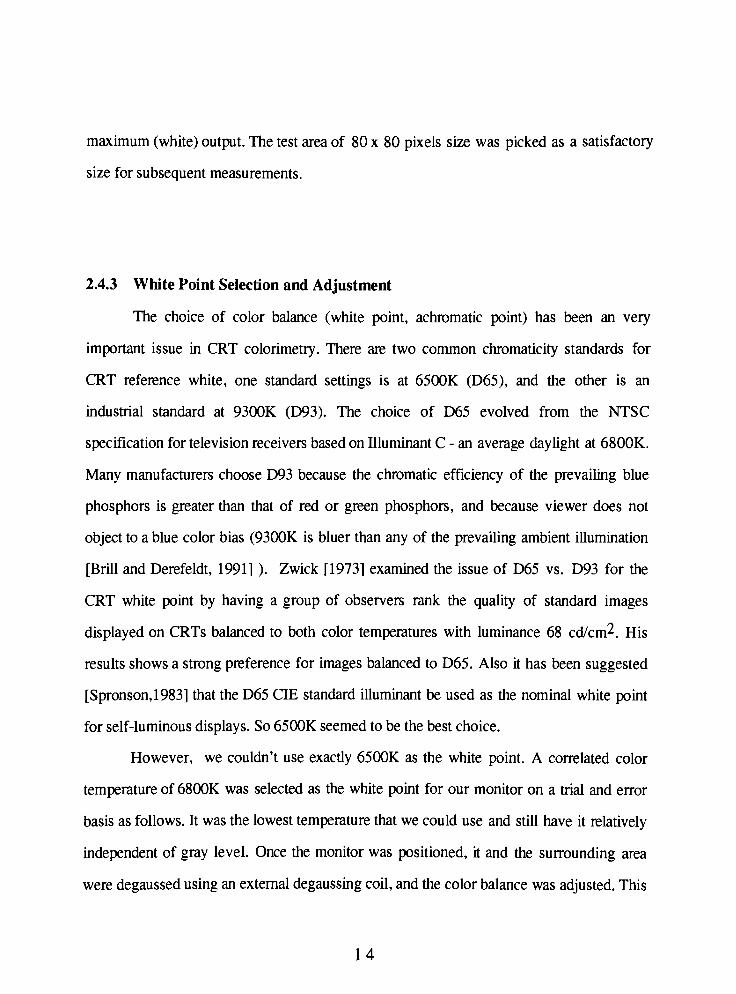
2.4.3 White Point Selection and Adjustment

The choice of color balance (white point, achromatic point) has been an very

important issue in CRT colorimetry. There are two common chromaticity standards for

CRT reference white, one standard settings is at 6500K (D65), and the other is an

industrial standard at 9300K (D93). The choice of D65 evolved from the NTSC

specification for television receivers based on Illuminant C - an average daylight at 6800K.

Many manufacturers choose D93 because the chromatic efficiency of the prevailing blue

phosphors is greater than that of red or green phosphors, and because viewer does not

object to a blue color bias (9300K is bluer than any of the prevailing ambient illumination

[Brill and Derefeldt, 1991] ). Zwick [1973] examined the issue of D65 vs. D93 for the

CRT white point by having a group of observers rank the quality of standard images

displayed on CRTs balanced to both color temperatures with luminance 68 cd/cm^. His

results shows a strong preference for images balanced to D65. Also it has been suggested

[Spronson,1983] that the D65 CIE standard illuminant be used as the nominal white point

for self-luminous displays. So 6500K seemed to be the best choice.

However, we couldn't use exactly 6500K as the white point. A correlated color

temperature of 6800K was selected as the white point for our monitor on a trial and error

basis as follows. It was the lowest temperature that we could use and still have it relatively

independent of gray level. Once the monitor was positioned, it and the surrounding area

were degaussed using an external degaussing coil, and the color balance was adjusted. This

14

was accomplished by adjusting the internal individual amplifier gain and bias controls and

iterating between the peak white and a low luminance neutral while making chromaticity

measurements using theMinolta CA-100 CRT color analyzer. The bias control was used to

adjust the lower luminance level, the gain control for the high luminance level. The purpose

was to have a correlated color temperature near 6500K for the neutral image while having a

small color variation over the intensity ranges. The Ramtek color monitor hardware

reference manual was a useful reference on monitor setup. Using a white point of 6800K,

the measured correlated color temperature of gray test patches remained within a 10K range

for digital levels from 255 down to about 64, as shown in Table 2.1.

Table 2. 1 Color temperature (CT) and luminance (Y) measurements at different DAC

levels .

DAC 0 8 32 64 96 128 160 192 224 255

CT 6690 6700 6740 6790 6800 6800 6790 6790 6800 6800

Y(cd/m2) 4.89 6.72 15.1 32.9 58.1 91.8 134 184 240 301

2.4.4 Measurements and Results ofCIE Tristimulus Values for the CRT

There was a 80 x 80 pixel size measurement window in the middle of the display

and the remainder of the display was set to gray with the luminance factor of 0.35 relative

to the peak white. The xyY mode of theMinolta Analyzer was chosen to measure the data.

In xyY display mode, values for x and y are CIE chromaticity coordinates and Y is

luminance, where x=X/(X+Y+Z), y=Y/(X+Y+Z) and z=(l-x-y). The measured xyY

values are easily transformed to CIE tristimulus values XYZ using X=Yx/y and Z=Yz/y. A

set of data consisted of 3 measurements for the individual red, green, and blue channels at

15

the maximum digital input 255. This data set contained primary chromaticity information

and was used to accomplish linear transformation between CRT tristimulus values and

CIE tristimulus values . The chromaticity measurements of three primaries are listed in

Table 2.2.

Table 2 . 2 The chromaticity measurements of the three RamtekCRT primaries.

Primaries x y Y(cd/m2) X Z

Red 0.600 0.347 72.8 125.9 11.1

Green 0.283 0.599 205.3 97.0 40.5

Blue 0.149 0.079 26.8 50.6 262.3

White 0.306 0.341 293.7 263.2 303.6

Given the linearity assumption, the resulting matrix for transform from RGB to

XYZ and the inverse matrix are :

125.9314 97.0117

72.8 205.25 26.75

11.0669 40.5358 262.3198

(2.7)

0.0109 -0.0048

-0.0039 0.0067 0.0001

0.0001 -0.0008 0.0039

(2.8)

16

2.4.5 Measurements and Results for the D-DgD,, to RGB Transformation

A set of 17 neutral images, which had equal digital value increments of 16 in the

range from 0 to 255, was measured in xyY units and was first transformed to XYZ values,

then was transformed to RGB space using Eq. (2.8). This data set was used to estimate

the parameters of the nonlinear relationship between DAC values and CRT tristimulus

values RGB. The parameters of the nonlinear relationship between the DAC D^D,, values

and the CRT tristimulus values RGB for the Ramtek monitor were estimated using the

regression program SYSTAT [1986].

R= 0.967*A.255

D.

1.845

+ 0.018

G= 0.969*- +0.016

I 255.

1.771

DLB= 0.971*-=-*- +0.018

255.

1.840

0<R<1

0<G<1

0<B<1

(2.9)

Inverting the relationship, we get the equations for the model digital outputs of the

RGB channels.

DQ18)1

r

10.967/'

f_255\G_0016)* 1,0.969/

'

D f^L\B-o,oisfb

V0.971/

0<R<1

0<G<1

0<B<1

(2.10)

17

Figures 2.1a to 2.1c shows the comparison between XYZ measured and model

values for the 17 neutral test patches.

400

300-

X200-

Measured X

Estimated X

100-

DAC Value

Figure 2. la Tristimulus value X vs. DAC value ofmeasurements and the model.

400

300-

200- Measured Y

Estimated Y

100-

DAC Value

Figure 2.1b Tristimulus value Y vs. DAC value ofmeasurements and the model.

18

400

300-

2. 200-

Measured Z

Estimated Z

100-

256

DAC Value

Figure 2. lc Tristimulus value Y vs. DAC value ofmeasurements and the model.

2.4.6 TestMeasurements over the CRT Gamut and Model Performance

A data set of 125 color samples uniformly distributed over the CRT color gamut in

a 5 x 5 x 5 grid pattern in DrDgDb space was measured. The xyY measurements were first

transformed to XYZ values and then toL'a'b*

values using Eq. (2.11). These 125

measurements were used for two purposes. First, they were used as the test data to

evaluate the accuracy of the CRT model. The second purpose was to determine the CRT

color gamut in CIELAB space.

19

L*

= 116*(

1/3

-16

/

a=500*

b'

= 200*

'( v V/3

\X*J

f v "\1/3

v^,

fry fz^i1/3

v^y V^.7

(2.11)

AE*

Histogram

The 125 test color patches were used to evaluate the performance of the CRT

model. The difference(AE"

value) between the measured and modelLVb*

data was

calculated for each patch. The averageAE*

was 2.27 and maximumAE*

was 5.36.

Figure 2.2 shows the error distribution in histogram form.

35 t"

m o in o in o w o in o m

o1- *-

CM CJ CO CO^,t in in

o w o in o w o w o in o

T-'-CMCMcoco^-'tf-in

delta-E*

Fig. 2.2 The histogram ofAE*

error distribution for the 125 color test patches

20

CRTColorGamut in CIELAB Space

CRT color gamut in T>ppb digital space was a cube shape. In order to visualize

color scales in CIELAB space, it was necessary to know the CRT color gamut in that

space. The 125 color sample measurements were transformed to show the CRT color

gamut in CIELAB space. The cube shape CRT gamut in D,DgDb space was changed, the

six original planes became six irregular curved surfaces as shown below. White is the

highest point and black is the lowest point. Both these points are on theL"

axis.

L*

a

Fig. 2.3 CRT color gamut in CIELAB space

21

Chapter 3 Pseudocolor Scales

3.1 Introduction

A pseudocolor scale is simply a trajectory in color space. An infinite number of

possible scales exist. In order to reduce the number, it was necessary to use some guiding

principles. After consideration of the literature, the following constraints on trajectories

were selected:

(1) the color gamut must be achievable on a CRT, which means the scales must be

inside the CRT color gamut.

(2) given the 8 bit display memory and 8 bit lookup tables, the scale will have 256

levels with the lowest level equal to black and the highest level equal to white.

(3) the scale should progress in a quasi-continuous manner through CIELAB space.

(4) perceptual linearity - each step on the scale should represent the same Euclidean

distance in CIELAB space (sometimes violated, more below).

(5) the lightness of the scale should increase linearly, which means lightness

changes equally with the each step on the scale.

(6)hue angle changes are equal increments around the lightness axis of the color

space.

(7) the step size in CIELAB space should be maximized.

The basic idea used for pseudocolor scale selection in this work was to find some

trajectories in CIELAB uniform color space satisfying the above constraints. Then using

the CRT calibration results, these trajectories could be transformed back to CIE tristimulus

XYZ space, to CRT tristimulus RGB space, and finally to 3x256 lookup tables in D,D Db

space. According to the first constraint mentioned above, the color scale must be achievable

22

on a CRT . In other words, in CIELAB space, the trajectory should be inside the CRT

color gamut. As we have already seen, the cube shape CRT color gamut in D,DgDb space

became an irregular shape (six planes become six curved surfaces) gamut in CIELAB

space. Using the CRTL*a*b*

data set of 125 measurements, the mathematical models of

these six curve surfaces could be estimated. The six surfaces in CIELAB space separately

corresponded to Dr =0, Dr =255, Dg=0, Dg=255, Db=0, Db=255 planes in the Dpph

space. The six surfaces can be divided into two levels. The three surfaces in the higher

level represented the Dr=255, Dg=255, Db=255 planes. The intersect of these three upper

surfaces gave the white point (255, 255, 255). The three surfaces in the lower level

represented D=0, Dg=0, Db=0 planes. The intersect of these three lower surfaces gave the

black point. The color trajectories must be found inside this CRTL*a*b*

gamut. In

CIELAB space, the color differenceAE*

between two points is represented by the

* / *2 +2 $2

Euclidean distance, AE =\AL +Aa +Ab . Perceptual linearity means equal AE

change for each step.

First, three commonly used color scales that we evaluated will be introduced to

familiarize the reader with the terms and concepts. Later we will describe ten novel scales

developed during this research. They are five constant AE scales and five variableAE*

scales that satisfy the constraints. Equal luminance and hue angle changes were required for

each step on the scales. The variableAE*

scales had gaussiar

The scales were spirals from black to white in CIELAB space.

each step on the scales. The variableAE*

scales had gaussian and triangleAE*

profiles

23

3.2 The Most Commonly Used Color Scales

32.1 The Gray Scale

The most commonly used scale is the gray scale. While not usually considered to be

a color scale, it is realized by traversing the color space along theL*

axis. This can be

achieved by keeping equal digital intensities for the three primaries T>ppb and increasing

them linearly from 0 to 255, as shown in Fig. 3.1. The digital level is the lookup table

address (input value from display memory) and digital intensity is the lookup table outputs.

256-

Fig. 3.1

192-

e0.

"3d

5

128-

Dr

Dg

Db

64-

256

Digital Level

Three DrDgDb digital intensities of gray scale. The linear variationof the three lookup table outputs (digital intensity) as a function of

input (digital level) from display memory.

3.2.2 The Rainbow Scale

Just like the physical rainbow, this scale contains all the hues of the rainbow

spectrum. In the CIE chromaticity diagram, the natural rainbow scale follows the boundary

of the pure spectrum (see Figure 3.2) . The realizable color scales are inside the triangle of

the CRT color gamut. The rainbow pseudocolor scale was suggested by Andrews, Techer

and Kruger [1972]. It is achieved by changing the three digital intensities D,DgDb as shown

in Fig. 3.3.

24

Fig. 3.2 CRT primaries in 1931 chromaticity diagram. RGB are the three

primaries of the CRT and w is the white point.

SiG

a

'

5

256-1

Dr

Dg

Db

Digital Level

Fig. 3.3 Three vppb digital intensities of the rainbow scale suggested byAndrews, Techer and Kruger [1972].

25

3.2.3 The Hot Body Scale

The hot body (heated-object) scale uses the colors that an object radiates as its

temperature increases. Ideally the scale in the chromaticity diagram should have the same

chromaticity coordinates as an blackbody radiator. ITie set of color temperatures ranging

from 0 to infinity is the complete hot body spectrum. It passes from infrared through red,

orange, yellow, and white. The hot body scale is achieved by bringing the CRT three

DrDgDb digital intensities up in the order red, green, blue as shown in Fig. 3.4. These data

were obtained from Levkowitz [1988] who got them from Chan [1983].

/ ) i

P ' i/ r

192- y j

y f '

> f J Iy ,

M

aj* * '

4- 128- / * '

e /*H / ^ /

a / -

r

i-m i * '

"53d 64- 'r i

?

5 <

iii

Dr

Dg

Db

64 128 192 256

Digital Level

Fig. 3 .4 Three DTD Db digital intensities of the hot body scale, Chan [ 1983]

26

3.3 Basic Principles for Generating ConstantAE*

Color Scales

These new scales were developed for this research work and were designed using

the constraints described in section 3.1 above. One set of 5 scales used constant step of

AE The scales were spirals in CIELAB space with constant AL*< Ah andAE*

for each

step. The valueAL*

was defined by (Lw*- L*b) / 255 according to the constraint 4, where

I_w was the luminance of white for the CRT and L*b was the luminance of black for the

CRT. The value of Ah was defined by (total angle / 254), since step 0 and step 255 were

on theL*

axis and there were 254 steps to complete the total hue angle. Three different

total angles were used (360,540

and 720). The value ofAE*

for each scale was

selected by finding the spiral starting angle angle that maximized the realizable dynamic

range of the perceptual difference. It was determined using the method described in the

following paragraphs.

The method of finding the maximum possible value ofAE*

for a given start angle

was iterative and proceeded as follows. The calculations were done using a computer

program written especially for this purpose. The source code is given in the appendix B.

The plane of the first luminance level, Li*= (L*b + AL ), intersects the CRT gamut with

a triangle-like boundary that projects onto the plane as shown in Fig. 3.5. Recall that

the CRT gamut boundaries in CIELAB space are actually curved planes.

27

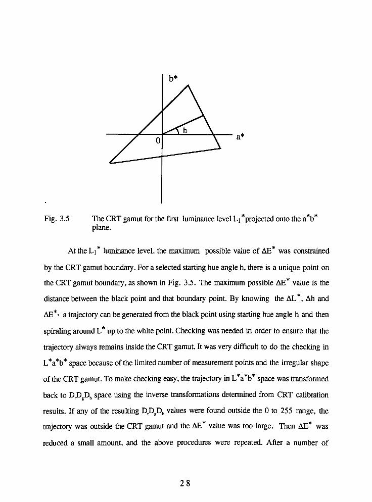
Fig. 3.5 The CRT gamut for the first luminance level Li *projected onto thea*b*

plane.

At theLi*

luminance level, the maximum possible value ofAE*

was constrained

by the CRT gamut boundary. For a selected starting hue angle h, there is a unique point on

the CRT gamut boundary, as shown in Fig. 3.5. The maximum possibleAE*

value is the

distance between the black point and that boundary point. By knowing the AL*, Ah and

AE*- a trajectory can be generated from the black point using starting hue angle h and then

spiraling aroundL*

up to the white point. Checking was needed in order to ensure that the

trajectory always remains inside the CRT gamut. It was very difficult to do the checking in

L*a*b*

space because of the limited number ofmeasurement points and the irregular shape

of the CRT gamut. To make checking easy, the trajectory inL*a*b*

space was transformed

back to DrD Db space using the inverse transformations determined from CRT calibration

results. If any of the resulting D,D_Db values were found outside the 0 to 255 range, the

trajectory was outside the CRT gamut and theAE*

value was too large. ThenAE*

was

reduced a small amount, and the above procedures were repeated. After a number of

28

iterations, a trajectory was found that remained inside the CRT gamut. The resultingAE*

value was themaximumAE*

at that starting hue angle. The whole procedure was repeated

360 times at different starting angles giving a sequence of maximumAE*

values as is

illustrated in Fig. 3.6 below. The largestAE*

among the 360 alternatives was the one

which gave the largest dynamic range for that scale. For the scale shown in Fig. 3.6, the

best starting hue angle is 175. Knowing the starting angle h , AL*, AE*, and Ah, the

trajectory was completely defined inL*a*b*

space and was transformed back to Dppb

space. This gave a 3 x 256 digital output lookup table for the color scale as shown in Fig.

3.7 below.

3.4 ConstantAE*

Scales

*

Five color scales were developed with constant AE increments. Three of the

scales were counterclockwise spirals aroundL*

and two were clockwise spirals. The three

counterclockwise scales had total angles of 360,540

and720

respectively. The two

clockwise scales had total angles of 360and 540. All scales started at black, spiraled

around theL*

axis inL*a*b*

space and ended at white. A summary of the scale parameters

that give maximum values of total AE are listed in table 3.1. The five scales are described

in detail in the following sub sections, and are shown in photographs in appendix A.

29

Table 3.1 Summary of constant AE scale parameters

scale name starting angle h AhAE*

calculated

totalAE*

measured

totalAE*

C360_ccw175 1.42

1.645 419 408

C540_ccw20 2.13

1.615 412 416

C720 ccw200 2.83

1.615 412 436

C360_cw90

1.594 406 398

C540_cw270

1.573 401 405

The measured total AE value was obtained by measuring xyY values of 32 levels

which were uniformly distributed through the scales and transformed toL*a*b*

values.

TheAE*

was calculated between these 32 points and added theAE*

together. The

differences between the calculated totalAE*

and measured totalAE*

values were due to

errors in CRT modeling. The model did not fit measurements particularly well at low

luminance values.

30

3.4.1360

Counterclockwise ConstantAE*

Scale (C360_ccw Scale)

Figure 3.6 shows how totalAE*

changed with different starting angles for the

360

ccw scale with fixed AE*. The best choice of starting angle of the scale was found to

be 175; Ah equals1.42

and AE*max equals 1.65 . The maximum totalAE*

is 419. It

was achieved by changing the D_DgDb digital intensities as shown in Fig. 3.6.

600'

t i i t r

60 120 180 240 300 360

Starting Angle

Fig. 3.6 TotalAE*

vs. starting angle (C360_ccw scale)

256

Dr

Dg

Db

Digital Level

Fig. 3.7 DrD Db digital intensities of the C360_ccw scale

31

3.4.2540

Counterclockwise Constant AE Scale (C540_ccw Scale)

Figure 3.8 shows how totalAE*

changed with the different starting angles for the

540

ccw scale with fixed AE*. The best starting angle for the scale was found to be 20;

Ah equals2.13

and AE*max equals 1.62. The maximum totalAE*

is 412. The scale was

achieved by changing the D_DgDb digital intensities as shown in Fig. 3.8.

600

9

3e2

t i i i r

60 120 180 240 300 360

Starting Angle

Fig. 3.8 Total AE vs. starting angle (C540_ccw scale)

256

>,192-

Vi

flv-*_*

fl

n4-1

"3d

128-

64-

r64 128 192 256

Digital Level

Dr

Dg

Db

Fig. 3.9 D^DgD,, digital intensities oftheC540_ccw scale

32

3.4.3720

Counterclockwise ConstantAE*

Scale (C720_ccw Scale)

Figure 3.10 shows how totalAE*

changed with the different starting angles for the

720

ccw scale with fixed AE*. The best starting angle was found to be 200; Ah equals

2.83

and AE*max equals 1.62 . The maximum totalAE*

is 412. The scale was achieved

by changing the DrDgDb digital intensities as shown in Fig. 3.1 1.

500-

*

8400-

A3300-

200-

100-

)<xiaatff^ ^bout**?

l i i i i

0 60 120 180 240 300 360

Starting Angle

Fig. 3.10 TotalAE*

vs. starting angle (C720_ccw scale)

256'

>>192-

tfi

fla*_

flHH

*5

*3>

128-

Dr

Dg

Db

64 128 192 256

Digital Level

Fig. 3.11 DrD Db digital intensities of the C720_ccw scale

33

3.4.4360

Clockwise ConstantAE*

Scale (C360_cw Scale)

Figure 3.12 shows how totalAE*

changed with the different starting angles for the

360

clockwise constantAE*

scale . The best starting angle of the scale was found to be

90; Ah equals and AE*max equals 1.59. The maximum totalAE*

is 406. It was

achieved by changing the T>ppb digital intensities as shown in Fig. 3.12.

600

Fig. 3.12

-i i 1 i r

60 120 180 240 300 360

Starting Angle

TotalAE*

vs. starting angle (C360_cw scale)

256-

^192-

</i

fl

it*_

*5ii

5

Fig. 3.13

128-

64-

i-LT-

256

Dr

Dg

Db

0 64 128 192

Digital Level

DrD Db digital intensities of the C360_cw scale

34

3.4.5540

Clockwise ConstantAE*

Scale (C540_cw Scale)

Figure 3.14 shows how totalAE*

changed with the different starting angles for the

540

clockwise constantAE*

scale. The best starting angle for the scale was found to be

270; Ah equals and AE*max equals 1.57 . The maximum totalAE*

is 401. It was

achieved by changing the D_D Db digital intensities as shown in Fig. 3.15.

600

H200

Fig. 3.14

i 1 1 i r

0 60 120 180 240 300 360

Starting Angle

TotalAE*

vs. starting angle (C540_cw scale)

256

V3

fl

es

"5b

5

Fig. 3.15

256

Dr

Dg

Db

0 64 128 192

Digital Level

DrD Db digital intensities of the C540_cw scale

35

3.5 Basic principles for generating variableAE*

scales

Two factors led to development of particular variable AE scales. One consideration

*

was that the constant AE scales did not use the maximum saturation colors available inside

the CRT gamut. Since the goal was to determine whether some color scales could increase

human visual signal detectability comparing to gray scale, we would like the color

trajectory to use as much of theL*a*b*

space as possible. The particular methods of

varying AE were selected based on the following consideration. The human observer

experiments used a signal detection task with a statistically defined (lumpy) background.

The probability distribution function (PDF) of the lumpy background level was a gaussian

function with a mean of 127 and a standard deviation of 32. We attempted to match this

*

PDF by weighting the values ofAE to give peak ofAE near the mean of the background

PDF. Therefore, biased gaussian and triangle AE functions were used in the scales. For

each step i, we again used AL =

(Lw*

-Lb*)/255 and Ah = 360/(256 -2). The

variation of AE is described by Eq. (3.1) for the gaussian scales and Eq. (3.2) for the.

triangle scales.

Equation (3.1) describes a biased gaussian function with a mean, u., equal to 127

and a standard deviation, o, equal to 40 or 60. The constant, B, is the offset value of the

biased gaussian function when i equals zero. This B value is to compensate for the non

zero value for the gaussian function at the first step. The value ofB is 0.006 for o equal to

40 and 0. 106 for a equal to 60.

( -a-

id

A*[i] = A*[0] +(A*[127]-AE*[0])* 2,

- B(3.1)

Equation (3.2) describes a biased triangle function centered at step 127.

aitVi-*

iE*[ni]-E*m)*i

A2_[,] = AE[0] +.<12?

.* AjAir_ (*[127]-*[0])*(/-127)

AE W = AE [127] .

> 12?

36

In both equations, AE*[0] equals to the maximumAE*

of the360

constantAE*

scale that we had previous found as a function of starting angle (see Fig. 3.6 and Fig.

3.12). The value of AE*[127] is the peakAE*

value at step 127. The method used for

generating the variableAE*

scales was very similar to the one for the constantAE*

scales.

In order to find the relationship between totalAE*

and starting angle, AE*[127] needed to

be determined for each possible starting angle. It was done by starting with AE*[127]

equal to AE*[0] for a given starting angle h and then increasing AE*[127] a small amount

for each iteration until the trajectory no longer remained inside the CRT gamut. To check

this, the trajectory was transformed into D^DgDj, space to see whether any data exceeded

255. This procedure was repeated for 360 different starting angles. When the value of

AE*[127] for every starting angles were found, the relationship between totalAE*

and

starting angle was determined. Figure 3.16 shows an example of howAE*

changed with

step number for the biased gaussianAE*

scale with standard deviation o equal to 40.

delta E*

256

stepi

Fig. 3.16 Biased gaussianAE*

vs. step number with o equal to 40

37

3.6 VariableAE*

Scales

Five variableAE*

scales were developed. Three were counterclockwise gaussian

AE*

scales, two with o equal to 40 at two different starting angles and one with o equal to

60. The fourth was a clockwise gaussianAE*

scale with a equal to 40. The last scale had

a counterclockwise triangleAE*

profile. All scales had total angles of 360, started at

black, spiraled around theL*

axis inL*a*b*

space, and ended at white. A summary of the

variableAE*

scale parameters are listed in table 3.2.

Table 3.2 Summary of the variableAE*

scale parameters

scale name

starting

angle h Ah AE*[0] AE*[127]

calculated

totalAE*

measured

totalAE*

G40_10_ccw10 1.42

0.639 2.019 299 269

G40_250_ccw250 1.42

0.679 4.179 518 467

G60 210 ccw210 1.42

1.295 2.335 453 481

Tri ccw210 1.42

1.295 2.255 453 454

G40 10 cw10

0.599 4.219 509 451

There are some differences between the calculated total AE and measured total

AE*. This is mainly caused by the error from CRT modeling. The model did not fit

measurements particularly well at low luminance values. We did not use the very low

luminance levels very frequently in the experiments. Since the background was below

digital level 64 only about 2.5% of display trials, the error did not substantially affect our

results.

38

3.6.1360

Counterclockwise GaussianDistribution AE Scales with o Equal to 40

(G40_250_ccw and G40_10_ccw Scales)

The profile of AE as a function of level number was a biased gaussian function

with o equal to 40. The relationship between totalAE*

and starting angle was shown in

Fig. 3.17. Two scales were chosen at very different starting angles. One scale had a

maximum total AE of 518 and starting angle of 250. The corresponding AE*[0] equaled

0.68 and AE*[127] equaled 4.18. The other scale had a totalAE*

of 299 and starting angle

of10

with AE*[0] equal to 0.639 and AE*[127] equal to 2.019.

600

i i i 1 r

0 60 120 180 240 300 360

Starting Angle

Fig. 3.17 TotalAE*

vs. starting angle(360

counterclockwise biased

gaussian profile forAE*

with o equal to 40 )

The two scales spiraled360

in the counterclockwise direction around theL*

axis.

The scale with starting angle of250

was achieved by changing three DrDgDb digital

intensities as shown in Fig. 3.18. Figure 3.19 shows the three digital intensities D_DgDb

changing in the scale with startingangle of 10.

39

256

Dr

Dg

Db

64 128 192

Digital Level

256

Fig. 3.18 DrDgDb digital intensities of the G40_250_ccw scale with a gaussian

AE*

profile with o equal to 40 and a starting angle of 250.

256

Dr

Dg

Db

64 128 192

Digital Level

256

Fig. 3.19 D_D Db digital intensities of the G40_10_ccw scale with a gaussianAE*

profile with o equal to 40 and a starting angle of 10.

40

3.6.2360

Counterclockwise Gaussian Distribution AE Scale with o Equal to 60

(G60_210_ccw Scale)

Figure 3.20 shows how totalAE*

changed with the different starting angles. The

best starting angle for the scale was found to be 210; AE*[0] equals 1.30, AE*[ 127]

equals 2.34 and the totalAE*

equals 453. The scale was achieved by changing the D_DgDb

digital intensities as shown in Fig. 3.21.

600'

9

3

i 1 i i r

0 60 120 180 240 300 360

Fig. 3.20

Starting Angle

TotalAE*

vs. starting angle (G60_210_ccw scale)

>>

'fiCii*j

fl

mm

03

'oi

5

256

192

128-

Dr

Dg

Db

256

Fig. 3.21

128 192

Digital Level

Three DTJ Db digital intensities of the G60_210_ccw scale

41

3.6J360

Counterclockwise TriangleDistributionAE*

Scale (Tri_ccw scale)

Figure 3.22 shows how totalAE*

changed with the different starting angles. "Die

best starting angle for the scale was found to be 210; AE*[0] equals 1.30; AE*[127]

equals 2.26. The totalAE*

equals 453. The scale was achieved by changing the D^-D,,

digital intensities as shown in Fig. 3. 23.

500-

SI400-

A1e2

300-

200-

100-

0- -

i i r

Fig. 3.22

60 120 180 240 300 360

Starting Angle

TotalAE*

vs. starting angle (Tri_ccw scale)

B

64-

"3d

5

256

192-

128-

Dr

Dg

Db

256

Fig. 3.23

128

Digital Level

D^ Db digital intensities of the Tri_ccw scale

42

3.6.4360

Clockwise Gaussian Distribution AE with o = 40 Scale

(G40_10_cw Scale)

The relationship between totalAE*

and starting angle is shown in Fig. 3.24. The

best starting angle for the scale was found to be 10; A9 equals -1.42; AE*[0] equals

0.60, and AE*[127] equals 4.22, and the totalAE*

is 509. It was achieved by changing

the DrDgDb digital intensities as shown in Fig. 3.25.

600-

500-

100-

0 I I I 1 1

0 60 120 180 240 300 360

Starting Angle

Fig. 3.24 TotalAE*

vs. starting angle (G40_10_cw scale)

256- 7T

/ \ / r

\ / *

1 t **

>>

"5fl

192-1 \

/ /1

a / \ / /-w 1 ' . f i

fl 128-

1 / \' * 1#

*

It \

*1

/

'l

/ /f

/ /

ct

1

/ /

"3d 64-

1 #

/ /

/

1/

Q

/x \ftp \ /

0- '

I 1 1

Dr

Dg

Db

0 64 128 192 256

Digital Level

Fig. 3.25 Three D-DgDb digital intensities of theG40_10_cw scale

43

Chapter 4 Psychophysical Experiments

4.1 Introduction

Visual signal detection experiments are done using samples from noise only

distributions and signal-plus-noise distributions. There are two main psychophysical

techniques [Green and Swets, 1988]. One is the Receiver Operating Characteristic (ROC)

method where a specified signal may or may not be present and the observer uses a rating

scale to express his or her confidence in a decision as to signal presence or absence. The

othermethod is the two-alternative forced choice (2AFC) method. In principle, the 2AFC

gives a direct measure of the observer's sensitivity since the experimental procedure

produces an average measurement over all possible decision criteria. The more general

MAFC approach with theM alternative images ( or portions of images ) is also occasionally

used for specific decision tasks when it is appropriate.

The 2AFC was chosen to evaluate the different color scales for particular signal

detection task here. The choice was based on the simplicity of doing and analyzing 2AFC

experiments in an accurate manner. A brief description of the method and the terminology

involved are given below and are exerpts from Burgess [1995].

4.2 The 2AFC Method

4.2.1 2AFC

The simplest of all forced choice experiments is a two-alternative detection task. In

the experiment, the observer is given two fields ofuncorrelatednoise in one image. One of

the two noise fields contains a signal with a known size, shape and intensity placed in a

44

know position. The other field contains only noise. The signal is randomly assigned to one

field or the other with equal prior probability. The observer is then asked to indicate (by

keyboard response) which of the two noise fields contains the signal. The optimum

decision strategy is that of the ideal Bayesian observer. The observer cross-correlates the

signal with the image data at the two alternative locations and uses the two cross-correlation

results as decision variables. In essence the observer is presented with samples from two

ideal-observer decisions, one is from the signal plus noise distribution and the other is from

the noise only distribution. The observer then selects the side with the higher decision

variable value. The experimenter determines the proportion of correct responses P for each

field and then calculates the detectability index d'.

4.2.2 Uncertainty Issues

A rigorous approach to signal detection theory makes a distinction between tasks

that are exactly defined and those that are statistically defined. This distinction is important

because the optimum decision strategies are quite different for the two cases. The simplest

case, signal know exactly / background know exactly (SKE/BKE), has a signal that is

known exactly (size, shape, possible locations ) and a background that is known exactly (

and usually is uniform). The only sources of uncertainty are additive white noise and the

random signal location assignment. For this task, the optimum detection strategy uses a

cross-correlation procedure and the detectability index for the ideal Bayesian observer

equals the SNR. Statistically defined tasks can have a variety of uncertainties [size, shape,

background] where the observer only knows the probability density functions of the

45

appropriate parameters. For these tasks, the optimum decision strategies are more complex

and the relationship between the detectability index and SNR will be nonlinear.

Experiments done using synthetic images are usually designed with uncertainty

issues in mind. Calculation of Bayesian ideal observer performance is straight forward for

the SKE/BKE case and mathematical intractable for the more general case of statistically

defined signals and background.

4.2.3 Selection of an Independent Variable

Many visual psychophysics experiments use signal contrast as the independent

variable. This approach does not take signal size into account. An alternative approach is to

use signal contrast energy. The signal has some spatially-variable contrast s(x,y) and

contrast energy is defined by

oo oo

E = J j[s(x,y)fdxdy (4.1)

oo oo

In medical imaging we are usually interested in noise-limited detection, so a more

appropriate parameter is the signal-to-noise ratio (SNR). For white noise with spectral

density N0, the definition is given bySNR2

= El N0. For discrimination tasks, the signal

to be detected is the difference between two signals, s{(x,y) and s2(x,y), and the signal-

to-noise ratio is calculated using

SNR2= ? ][sl(x,y)-s2(x,y)fdxdy = AE/Ne (4.2)

O oo oo

46

This calculation assumes uncorrelated (white) gaussian noise and the SNR

corresponds to the detectability index for the ideal (matched filter) observer doing the same

SKE/BKE task. One can do a similar calculation for detection and discrimination tasks in

correlated gaussian noise using the pre-whitening matched filter. The situation for

statistically defined signals and non-uniform statistically defined backgrounds is

considerably more complex. For statistically defined (lumpy) backgrounds, Barrett [1990]

has suggested the use of the Fisher-Hotelling optimum linear observer as a mathemetically

convenient standard for evaluation and comparison ofhuman observer performances.

4.2.4 Selection of a Performance Measure

In order to present results of observer experiments we need some measure of

performance. We would prefer a one-dimensional measure that relies on as few

assumptions as possible about the internal operations of the observer. In other words, we

would prefer a measure that is as model-independent as possible. We would also like a

measure that can be determined using a reasonably small number of decision trials. The

discussion here is restricted to two measures of theMAFC method.

MAFC performance can be described by the proportion, P, of correct responses

and by the detectability index, d'. The value of d can also be viewed simply as a

convenient transformation ofP. The particular transformation used depends on the value of

M. To be consistent one could use the notation d'M to make the M-dependence explicit .

This will not be done because detectability index results are usually presented in the context

of some experiment and the value of M is specified. The interpretation used here is

analogous to that of the z-score (normal deviates) transformation used in analysis of 2AFC

47

experiment. The z-score transformation is not useful for the general MAFC case, so the

d'(P) transformation approach is a useful alternative. For MAFC experiments, chance

performance gives P-l/M for equal priors.

Why should one want two measures forMAFC experiment? The problem lies in the

limited range of the P measures, and its compressive nature as their values approach unity.

As the amplitude of the signal to be detected increases (or alternatively the SNR increases),

equal increments in amplitude do not give equal increments in P. The relationship between

P and SNR would have a slope, dP/dS, that approaches zero as P approaches one. The

detectability index can be used to avoid this problem. One can viewd'

as measure designed

to scale in some reasonable fashion with SNR. If the SNR is zero, then one should expect

the detectability index to be zero. Similarly, equal changes in SNR should give

approximately equal changes in detectability index.

In the psychophysics literature one encounters many model-based interpretations

ford'

with associated subscripts. This multiplicity leads to confusion. If one's goal is to

construct or evaluate mathematical models of human observers, it would certainly

complicate the issue if one were to incorporate features of the model into one's measure of

performance. Therefore, the interpretation used here is simply this. The detectability index

d'

is nothing more than a real number obtained by a defined transformation of P for an

MAFC experiment. It is true that the transformations are derived using particular models

that requires assumptions. However, once the mathematical forms of the transformations

have been obtained, it is convenient to simply regard them as a way of obtaining a

performance measure with useful properties. The experimenter using this measure must, of

course, be always aware of that issues such as task selection and experimental design can

affect

d'

results. That is, there is some functional relationship betweend'

and SNR for the

48

task and associated parameters that are varied in the experiment. The purpose is to develop

models that explain and predict these relationships.

4.2.5 Calculation of theDetectability Index

The theory for analysis of signal detection experiments is based on the assumption

that the various sensory events involved in each alternative of the visual task can be mapped

onto a single dimension ( the decision variable ). For a 2AFC experiment, both signal and

noise samples are present in random order, so the two possible hypotheses are <sn> or

<ns>. For MAFC experiments there are M hypotheses, <snnn...>, <nsnn...>, <nnsn...>.

etc. In the most general analysis the choice among the M hypotheses is based on an

observation that is an M-dimensional vector of real numbers. It is necessary to know the

probability density function (PDF) and covariance function of this vector. These functions

are not directly observable and so must be inferred from the observer's decision data. In

practice, a number of simplifying assumptions are made about the PDFs.

The simplest assumption is that the alternative observation intervals are statistically

independent, that all PDFs are gaussian (normal), and that all variances are the same.

Statistical independence of the observation intervals in the displayed image is ensured by

careful experimental design. The assumption of the gaussian distribution is usually justified

theoretically by invoking the central limit theorem. It is assumed that the observer uses

internal decision variables that are composed of a multitude of smaller sensory events

which are approximately independent. At a practical level, the gaussian PDF assumption

introduces considerable mathematical convenience for analysis.

49

The analysis of 2AFC experiments is also based on the assumption of gaussian

PDFs. In a practical sense it does not matter whether the two decision variables have the

same variance. One view of 2AFC experiments is that the observer determines two decision

variable values (vi and V2, with variance a2\ and o22) and selects the alternative image

with the higher value ( assuming equal priors). If for some reason the variances are

unequal, one can do a change of variables. In the alternative view the observer calculates

the difference, v^ = vi- V2. The two alternative hypotheses about the state of the data,

(vi V2), are Hi = <sn> and H2 = <ns>. The observer selects Hi if Vd is positive and H2

otherwise. The two probability density functions have the same variance (o2=a2i+o2i).

The value ofd'

obtained from the proportion of correct responses does not depend on the

ratio of the variance.

The issue of possible observer bias in forced choice experiments is potentially more

serious. Response bias is the tendency of an observer to favor one response alternative

over the other. Any response bias in 2AFC experiments will, of course, reduce the

observer's performance because given equal priors the optimum decision procedure is to be

unbiased. It has been stated [Green and Swets, 1988] that the bias problem is much smaller

in forced choice experiments than in ROC experiment, especially at higher signal to noise

ratios. It is possible to obtain an"unbiased"

estimate of d'. As a matter of practice most, if

not all, visual psychophysics experiments are analyzed assuming unbiased observers and

usingd'= V2z(P) . The relationship between proportions, P, and the corresponding

z-

score is given by the integral of the cumulative normal distribution.

P(z) = <p(z)= -J= P

exP("*2

' 2M* (4'3>-J2nJ-x

50

The inverse relation is given by

z{P)= fl(P) (4.4)

The following method of calculating

d'

was used in this research to give an

unbiased estimate of

d'

[MacMillan and Creelman, 1991]. For each signal (3 different

amplitudes were used), the numbers of correct responses on the left, NLC , and right , NRC ,

were recorded along with the number of trials with signal on the left, NL, and right, NR.

The average proportions of correct responses on the left , PL, and right, PR, were

calculated, PL =N^ / NL and PR = NRC / NR. The value of the z-scores on the left, i^ , and

right, Zr , were calculated using Eq. (4.4). The average z-score was calculated using z= (t^

+ Zr ) / 2. The unbiased detectability index estimate is d'=V2z(P) . Thend'

for that signal

amplitude was normalized by SNR. There were three different signal amplitudes and hence

three SNRs randomly intermixed in each block of trials. The average d/SNR was

calculated using Eq. (4.5).

= IV-4- (4.5)-J *~l CAVDSNR 3 fx SNR:

51

4.3 Experiments for the Evaluation of Pseudocolor Scales

4.3.1 Goals

The aim of this research was to evaluate the human observer signal detection

performance with 12 different pseudocolor scales and compare to gray scale performance.

It was hoped that by careful design, pseudocolor scales could be found that would give

detection performance as good as or better than that obtained with a gray scale.

43.2 ExperimentalMethods

The experiments were performed using signals added to white noise and a

statistically defined (lumpy) background (an example shown in figure 4.1, page 54). Two

signals were used, a sharp-edged disc signal and a two dimensional gaussian signal.

Different sizes of the disc signal were evaluated. Two white noise spectral densities, N0,

were used. One was of 400 digital level2 / pixel2, which gave an amplitude standard

deviation of 20 digital levels. The other was 25 digital levels2 / pixel2 and the amplitude

standard deviation was 5 digital levels. The lumpy background was produced by low-pass

filtering white noise with a gaussian low pass filter to give a power spectrum of the form

W(f) = W0exp(-47t2s2f2), where s is the spatial standard deviation ( correlation distance ).

A value of s equal to 8 was used for most experiments and s equal to 16 was used for large

discs. The zero frequency value of the background spectral densities, W0 ,was selected to

give a background amplitude standard deviation of 32 digital levels.

The reason for using a lumpy background instead of a uniform background was to

explore a larger dynamic range of the scale. The signal amplitudewas only 5-10 digital

52

levels. The two white noise cases gave amplitude standard deviations of 20 and 5 digital

levels. With a uniform background, the signal plus noise distributions were always

centered at digital level 127 and little dynamic range of the scale would be explored. When

using the lumpy background of amplitude standard deviation o equal to 32, the signal plus

noise distribution in the vicinity of the signal varied over a wide range. The total amplitude

standard deviation of the noise plus lumpy background became approximately 37.7 and

32.4 digital levels for the two different noise cases respectively. A larger range of local

backgrounds was used in this case. About 32% of noise fields had a signal on a

background outside the 96 to 160 range of digital levels, and 5% of the noise fields had a

signal background outside the 64 to 192 range of digital levels. A total of 13 color scales

were evaluated for the disc signal with radius of 4 pixels and the gaussian signal with

spatial standard deviation of 3 pixels at the higher noise level (amplitude standard deviation

of 20 digital levels). Six color scales were selected to evaluate the performance at the lower

noise level (amplitude standard deviation of 5 digital levels). Three selected color scales

were further evaluated with three different sizes of the disc signal (radius of 4 pixels, 8

pixels and 12 pixels).

The images were displayed using a DEC MicroVax computer, a Peritek VCU-Q

display board, and a Ramtek GM-714 monitor. The display board was configured to give

240 x 320 pixels at a 60 Hz refresh rate (non-interlaced). Two same size image fields

(usually 32 x 32 pixels) were displayed side by side on the monitor. Both fields contained

white noise plus lumpy backgrounds. The signal was randomly assigned to one of the two

fields. Figure 4.1 shows an example image.

53

Fig. 4. 1 An example image of the signal detection experiment using the

display scale C720_ccw.

The image contains a display of the lookup table in use for the block of trials, two

fields (signal + noise + lumpy background) and a uniform gray surround at digital level

127. Reference copies of the disc signal are shown above the noise fields to illustrate size.

54

The signal is always centered in one of the noise fields. The SNR was set to 11.5 to make

the signal easy to detect in this illustration. The observations were done using the two-

alternative forced choice (2AFC) method in blocks of 256 decision trials with random

variation of experimental conditions between blocks. The viewing distance was fixed at 1 .8

meters using a chair with headrest. The observer selected left or right alternatives using a

one or two keyboard response. Three different signal to noise ratios were used for each

block of 256 trials with random amplitude selection. The three SNRs were selected to give

d'

in the range from 1.5 to 2.5. A linear relationship betweend'

and SNR was assumed.

The value ofd'

/ SNR was calculated by the method described in section 4.2.5. The signal

to noise ratio (SNR) was determined for the uniform background case.

All observers did three training blocks for each signal and lookup table ( color and

gray scales randomly selected ) to gain experience before experimental data collection

began. Three observers were very experienced with gray scale before this experiment. The

other three had never done this type of psychophysical experiment before. A total of 768

decisions trials were used for each condition in the experiments, giving a coefficient of

variation of 5% on estimates of the d'/SNR ratio [Burgess, 1995]. Six observers took part

in the experiment and thirteen pseudo-color scales were evaluated (including the gray

scale).

4.3.3 Experimental Results and Discussion

Disc Signals

The human performance for each color scale was first evaluated usingd'/SNR (the

ratio of detectability indexd'

and the signal to noise ratio). Figure 4.2a shows these results

55

for the disc signal with radius of 4 pixels in white noise (amplitude standard deviation of 20

digital levels) added to a lumpy background. The six observers had systematically different

performance when averaged across all 13 display scales. We were interested in observer

variation with the different display scales. Therefore, it seemed reasonable to normalize

each observer's performance

(d'

) relative to his average across scales

(davg'

) for that

experimental condition (signal type and noise level). Hence we will also show normalized

detectability, d7davg'

, for each observer and each display scale. Figure 4.2b shows these

relative results for the data previously presented in Fig. 4.2a. Note that removing the

systematic differences between observers decreases the dispersion of the data for nearly all

display scales. These two kinds of data presentation will be used for all experimental

conditions. The first figure type(d'

/ SNR) is presented for completeness. Attention should

be focused on the second figure type (d7davg'

)

Figures 4.2a and 4.2b show that average performance with the hot body scale is

almost as the same as the gray scale. The performance with the counter-clockwise gaussian

scale (G40_10_ccw) is the second best for color scales. The signal detectability with the

other color scales is lower than with the gray scale by about 20%. Performance is the

worst with the rainbow scale and is only about 1/3 of gray scale performance. For each

scale, the performance of the six observers is slightly different. The performance of some

observers with some color scales are slightly higher than with the gray scale. There are 5%

error bars applied to data for one of the observers in both figures. Note that observers are

generally consistent with oneanother.

56

c/_

0.5-i

0.4

03-

0.2-

0.1-

0.0-

I1 *l

I

Mi*-, t*s .

1A

X

a

6.

table name

el

"I

>.

o

o__

T-T-

TT"

*

1 TT"T-

*0 u o u u u u u 0

o__

e

u u u

Ju u

1

u

11

e ou e

o a ve t rH

*N . PN 1

X tf r> IO r- I n n

U U U 1 1 Tft r _

i

r

o u

I I

ve T

f> IT)

u u

AB

rH

HL

YQ

YZ

WZ

average

O t vew

O O

Fig. 4.2a Disc signal detectability normalized by SNR in high amplitude noise. Note

consistency of the observers with one another across the scales

2.0-,

1.5-

Ml>

L__J

b1.0-

a

0.5-

0.0-

wV^

Itable name

i i i i i r-i i i i r

+ AB rel ave

X DH rel ave

HL rel ave

D YQ rel ave

A YZ rel ave

V WZ rel ave

AVG rel ave

_O _s

o o

I I I I

N C ^

oooo o o o

_eo u o oooo

B ' ' '.-. -z

qa ve ^ s t,

w (j n w h-_

*W O U '

_

> <w

^ rgt ve

w

U U

Fig. 4.2b Disc signal detectability relative to the averaged'

for each observer.

Note the reduced variability of the data formost scales.

57

Six scales were selected to be further investigated in the lower noise level. An

example image at low white noise is shown in Figure 4.3. Figures 4.4a and 4.4b illustrate

the performance of six observers for detection of the disc signal (radius of 4 pixels) in

white noise with amplitude standard deviation of 5 digital levels.

The results are consistent with those for the higher noise level. The performance

with the gray scale is slightly better than with the hot body scale. But the difference may

not be significant. Again performance is worst with the rainbow scale. The results are

consistent between observers. In Fig. 4.4b, note that removing the systematic difference

between observers decreases the dispersion of the results for most display scales and the

scale differences becomes more clearly seen.

Figure 4.3 An example image at low noise level using the hot body scale.

58

OJ-, -A

-b

0.2-

0.1-

0.0-

6.. xX

X.g3.

A

+

jr

+

+

v

table name

au

tf

>.

1

i

1 1

*

0o o o o

__

o o

B 1 1

ITa ve i/> V>

X tf rr,

U

rl

tf

W

AB

DH

HL

YQ

YZ

WZ

average

Fig. 4.4a Disc signal detectability normalized by SNR in lower amplitude noise.

2.0-i

>

1.5- J.

% 1.0-

-b

0.5^

0.0-1r

AB rel avg

tr

1 * *

* *

table name

ah

tf

11-

o

__

B

e__

o

ae tf

T"

o

o

ve

rr,

U

T-

o

o

I

tf

T-

o

i/>

U

X DH rel avg

HL rel avg

a YQ rel avg

A YZ rel avg

? WZ rel avg

" AVG rel avg

Fig. 4.4b Disc signal detectability relative to the averaged'

for each observer in

lower noise. Note the reduced variability of the data for each scale and

the consistency of the observerswith one another across the scales.

59

Gaussian Signals

Figures 4.5a and 4.5b show the signal detection performance of six observers over

the 13 scales for the gaussian signal with spatial standard deviation of 3 pixels in white

noise (amplitude standard deviation of 20 digital levels) and a lumpy background. The

performance with color scales was almost always lower than with the gray scale. Among

these color scales, the detectability with the hot body scale was usually the highest. The

performance with the rainbow scale was always far below other scales and only about 1/3

of gray scale performance. For some experienced observers, the detectability of several

color scales was sometimes a little bit higher than the average gray scale. But statistically,

no conclusion could made from that. Note that removing the intra-observer variability (Fig.

4.5b) decreases the dispersion of the results for each scale and the scale differences are

seen more clearly. The observers are generally consistent with one another.

Six scales were selected to be further investigated in lower noise. The detectability

performance of the six observers over the 6 scales for the gaussian signal in white noise

amplitude standard deviation of 5 digital levels is shown in Fig. 4.6a and 4.6b. Again the

results are consistent with the ones in higher noise level. The performance with the gray

scale seems to be slightly better than with the hot body scale, but the difference may not be

significant. The performance with the gray scale and the hot body scale is significant higher

than with other color scales. The detectability with the rainbow scale is only about 1/6 of

the detectability with the gray scale. There are 5% error bars applied to data for one of the

observers in the figures. Note that observers are generally consistent with one another.

In general, the performance with the disc signal was better than it was with the

gaussian signal. The difference between the performance with disc and gaussian signals

was larger in high noise than it in low noise. Comparing the results with high and low

60

noise level, the performance with 400 digital level 2I pixel2white noise was better than it

was with 25 digital level2/ pixel

2white noise for both disc signal and gaussian signal

cases.

61

_

b

0.4-,

0.3-

0.2-

0.1-

0.0-

Ui

x i - _

+ + i

Ktable name

WTTTTTTTTTTTEUoooooooooooWaOOOOOOO

tf _a

o ve * m

* Ot rr> >r> t-

*W U U

I I I I I I I

' ~ "

y yI <s r

_

I I ^tTt rn

O Tt vew

tf tf

+ AB

X DH

HL

D YQ

A YZ

V WZ

average

Fig. 4.5a Gaussian signal detectability normalized by SNR in high amplitude noise.

2.0-1

5, 1.0-1

b

*0.5H

0.0-

1.5H"-

*1 ?

.'A

_

_*__!

D

table name

*

AX A

fl-JD

n r i ii

* * *o o o

o o o

I I I._:

S a ve tt n

- ;< f> /. r-

*y u v

>> >. *"o 5

^ o z

tf **

Tr

1 I I I r

*******o o o o o o o

oooo IIII I I I

* v rr

I rr, v>

y y

b. wi

"^I W "

I

rj tt ve

tf tf

tf

+ AB rel ave

X DH rel ave

HL rel ave

D YQ rel ave

A YZ rel ave

7 WZ rel ave

AVE rel ave

Fig. 4.5b Gaussian signal detectability relative to the averaged'

for each observer in

high amplitude noise. Note the reduced variability of the data for each scale.

62

0.2-,

Z

0.1-

0.0-

*-a_>

tf

_B

1

o

o

o

BC

#

i

table name

T"

*o

JO

B

a

tf

*o

o

I

ve

U

T"

*o

o

Tt

tf

*o

I

Tf

tr,

U

+ AB

X DH

HL

D YQ

A YZ

V WZ

average

Fig. 4.6a Gaussian signal detectability normalized by SNR in low amplitude noise.

2.0^

V

+

X

AB rel avg

DH rel avg1.5-

A -....

HL rel avg0X1>08i__j

1.0-A

D YQ rel avg

b #_

**. *

_

vA YZ rel avg

-b 0.5-#

#

*

V WZ rel avg

table name

n n...-J.... AVG rel avgU.U-1

1 1 i

* *

1

*

1

*a o

o o o o_

tf0__

__

o

1

o

Tf

oa ve ** WI

X tf p.

UTt

tf

U

Fig. 4.6b Gaussian signal detectability relative to the averaged'

for each observer in

lower noise. Note the reduced variability of the data for each scale.

63

Size DependenceExperiment

The CIELAB space was based on color discrimination differences with2

test

areas. This is considerably larger than the signal sizes used in the above experiments. For

our experiment setup, one pixel was about 0.43 milliradians (0.025) of visual angle. The

disc signal with a diameter of 8 pixels subtended only0.2

visual angle. This is a very

small visual angle relative to that used in color discrimination tasks to define the standard

observer. So we had to determine whether performance with color scales improved for

larger signal diameters. This size dependence experiment was done only for the disc signal

case. Based on the previous experiments, three scales were chosen to be investigated. They

were the gray scale, the counter clockwise360

constant AE scale (C360_ccw) and the

clockwise540

constant AE scale (C540_cw). Three different sizes of the disc signal were

tested. One was diameter of 8 pixels, the other two were diameter of 16 pixels(0.4

visual

angle) and 24 pixels(0.6

visual angle). The field size was changed from 32 x 32 pixels to

64 x 64 pixels and the spatial standard deviation of the background was changed to 16

pixels. Figure 4.7 shows the average performance of the six observers for the three

different disc sizes.

64

0.4-

+

0.3- X

zc/_ 0.2- +

-b

0.1-

00

R+

H

l

8

1

16

diameter (pixels)

1

24

+ Gray

X C360_ccw

C540 cw

Fig. 4.7 Average disc detectability normalized by SNR for 6 observers with

three different signal diameters and 3 color scales.

It was obvious that the detectability of 8 pixels size signal was the highest. The

largest size signal was the worst. In all cases the performance with the gray scale was the

best. The detectability with the color scales was always lower than with the gray scale.

There was no significant different between performance with the two color scales. This

indicated that the different sizes of disc signal had no effect on the conclusion that the

performance with color scales was worse than with the gray scale.

43.4 Conclusions

In these experiments, we compared the detectability of signals with a variety of

display scales using disc and gaussian signals at two different noise levels (for 13 and 6

color scales respectively). Also the size dependence of the disc signal detectability was

investigated for three color scales. The results showed that performance with the gray scale

65

was always the best. The hot body scale was usually the best color scale and sometimes

was not significantly worse than the gray scale. The performance with the rainbow scale

was always far below performance with any other scale. Typically detectability was only

about 30% of gray scale performance. The performance with the other spiral scales were

quite close to each other and worse than with the gray scale and the hot body scale.

The size of the signal affected the detectability. The smallest signal gave the

highest performance and the largest signal gave the lowest performance. The main point to

note was that observer performance with the gray scale was always superior to that with

pseudocolor display for all signal sizes.

66

Chapter 5 Discussion and Future Research

5.1 Summary and Discussion

The Ramtek color monitor was calibrated using a two-stage model. The first stage

was a nonlinear transformation relating normalized DAC values to device-dependent CRT

tristimulus values RGB. The second stage was a linear transformation where the device-

dependent CRT tristimulus values RGB were transformed to device-independent CIE

tristimulus values XYZ. The ten new pseudocolor scales were first developed in CIELAB

space and then transformed to CRT digital D,DgDb space using the CRT calibration results.

A number of selected constraints were satisfied by the new scales. Equal luminance and

hue angle changes were required for each step on the scales. There were two types of the

scales, one had constant perceptual distance steps, AE*, and the other had variable

AE*

steps with gaussian or triangle profiles. The resulting scales were spirals around theL"

axis

from black to white in either clockwise or counterclockwise direction. The starting angles

were selected to give maximum perceptual dynamic range.

Thirteen scales were investigated in signal detection experiments using the 2AFC

method. These included the gray scale, the rainbow scale , the hot body scale and the ten

new developed color scales. Six observers participated the experiment. The signal

detection experiments were performed using disc or gaussian signals added to white noise

and a statistically defined lumpy background. The experiments were repeatedfor both high

and low noise levels. The observations were done in blocks of 256 decision trials with

random variation of experimental conditions between blocks. All observers did three

training blocks for each signal and lookup tableto gain experience before experimental data

67

collection began. A total of 768 decision trials were used for each condition in the

experiments. A size dependence experiment was performed for the disc signal at high noise

level. For the disc signal, the performance with the hot body scale was as good as

performance with gray scale in the high noise level. The performance was slightly worse

than with the gray scale in low noise level. But the difference may not be significant. The

performance with some spiral trajectory color scales (G40_10_ccw and C540_cw) was

just slightly lower than with the gray scale and hot body scale in high noise level. The

performance with other spiral color scales was about 20% and 30% lower than with the

gray scale in high and low noise levels. The detectability of the rainbow scale was the

worst and only about 30% and 15% of the gray scale in high and low noise levels

respectively. For the gaussian signal, the performance with the gray scale was always

better than with the color scales. Among the color scales, the detectability with the hot body

scale was usually the highest. The performance with C360_ccw spiral scale was slightly

lower than with the hot body scale. The performance with other spiral color scales was

about 25% and 38% lower than with the gray scale in high and low noise levels.

Performance with the rainbow scales was always far below other scales and only 30% or

15% of the gray scale performance in high or low noise levels. In the size dependence

experiment, we found that the smaller the disc signal, the better the performance. The result

also indicated that the difference sizes of disc signal had no effect on the conclusion that

the performance with color scales was worse than with the gray scale. The dynamic range

of the new CIELAB spiral color scales were all larger than that of the gray scale. But the

detectability of the gray scale was always better than those color scales. It seemed that the

larger perceptual dynamic range had no benefit on these kinds of noise limited signal

detection experiments.

68

Among the thirteen scales, the six observers felt most comfortable with the gray

scale. They also liked the hot body scale, G40_10_ccw scale and the C360_cw scale. It

seemed that they were comfortable with scales with less hue information. The observers

were generally consistent with one another across all of the experiments.

The results is not surprising. For signal detection, luminance information is most

important. It has been suggested that form detection by the human visual system is based

on the luminance changes. Color scales which contain a large amount of hue information

could cause observers to be less sensitive to luminance changes. The hot body scale retains

the advantages of gray scale in that the luminance increases monotonically and has

approximately the same color through the scale. So the performance is almost as same as

with the gray scales. The rainbow scale is very colorful, but the performance is the worst

among all the scales.We think this is because luminance of the rainbow scale changes non-

monotonically and there is very little luminance variation across the mid-range (near 127)

for this scale.

Although these pseudocolor scales were suboptimal for the signal detection tasks,

they are useful for purposes other than detection. Some example applications are amplitude

identification or classification. Color scales also allow users to discuss image amplitudes

since we have a common vocabulary for hues but have trouble conversing about gray levels

in an image.

69

5.2 Future Research

We feel that the results of our investigation lead to several directions for future

work. Some are given next.

1. Testing the new scales for accuracy of data amplitude identification. This is one

of the main benefits of pseudocolor scales.

2. The investigation of using these color scales in computer graphics (scientific data

visualization) is worth pursuing.

3. As previously mentioned, CIELAB space was used as the uniform color space,

and the color difference equation was based the standard CIELAB 1976AE*

Euclidean

distance. Some new color difference equations have been developed. Recently QE

recommended the TC 1-29 (CIE94) color difference equation [CIE, 1995]. The CIE94

color difference formula could provide better perceptual linearity than CIELAB.

4. One might try different constraints. For example, changing hue uniformly(AH*

is constant) over the 256 levels rather than hue angle. Recall thatAH*2= AE*2

-AC*2.

This may increase the complexity of the mathematical development of the scale. But it

would have the same hue step throughout the scale.

70

References

B. Alfano, A. Brunetti, A. Ciarmiello andM. Salvatore, "Simultaneous display ofmultiple

MR parameters with 'Quantitative Magnetic ColorImaging'

", J. Comp. Asst. Tomog. 16,

634-640 (1992).

H.C. Andrews, A.G. Tescher and R.P. Kruger, "Imaging processing by digital

computer", IEEE Spectrum 9, 20-32(1972).

H. H. Barrett, "Objective assessment of image quality: effects of quantum noise and object

variability."

J. Opt. Soc. Am. A 7, 1266-1278 (1990).

R.S. Berns, R.J. Motta and M.E. Gorzynski, "CRT colorimetry, Part I: Theory and

pratice", Color Res. Appl. 18, 299-314 (1993).

R.S. Berns, RJ. Motta and M.E. Gorzynski, "CRT colorimetry, Part II: Metrology",

Color Res. Appl. 18, 315-325 (1993).

R.M. Boynton, Human Color Vision. Optical Society ofAmerica (1992).

M. H. Brill and G. Derefeldt, "Comparison ofReference-White Standards for Video

DisplayUnits."

Col. Res. Appl. 16, 26-30 (1991).

71

A. E. Burgess, R. F. Wagner, R. J. Jennings, and H. B. Barlow,"

Efficiency of human

visual discrimination."

Science 214, 93-94 (1981).

A. E. Burgess, "Comparison of receiver operating characteristic and forced choice observer

performance measurement methods",Med. Phys. Vol. 22, No. 5 (1995).

E.C. Carter and R.C. Carter, "CIELUV color-difference equations for self-luminance

displays", Color Res. Appl. 8, 252-253 (1983).

F.H. Chan and S.M. Pizer, "An ultrasound display system using a natural scale", J. Clin.

Ultrasound 4, 345-348 (1976).

F.H. Chan, An ultrasound display device using pseucolor scale. Ph.D. dissertation, Univ.

ofNorth Carolina (1983).

CIE PublicationNo. 90, "CRT Colorimetry, a Bibliography", International Commission

on Illumination, Bureau Central de la CIE, Vienna (1990).

CIE Technical Report, "Industrial Color Difference Evaluation", CIE 1 16 (1995).

E.J. Crowe, P.F. Sharp, P.E. Undrill and P.G.B. Ross, "Effectiveness of color in

displaying radionuclide images",Med. andBiol. Eng. and Comp. 26, 57-61 (1988).

72

A.R. Doucette, "Color discrimination in digital displays", SID, Digest ofTechnical

Papers, P.48 (1977).

J.D. Foley and J. Grimes, "Using color in computer graphics", IEEE Comp. Graphics

andAppl. 8,25-27(1988).

R.S. Gallagher (Ed.), Computer Visualization. CRC Press (1995).

D. M. Green and J. A. Swets, Signal detection theory andpsychophysics (Wiley, New

York, 1966). Reprinted by Peninsula Publishing, Los Altos. CA. (1988).

A.S. Houston, "A comparison of four standard scintigraphic TV displays", /. Nucl. Med.

21,512-517(1980).

K. Kinameri andM.Nonaka,"

Measurements ofwhite uniformity of color picturetubes."

Appl. Optics 13, 1270-1272 (1974).

H. Levkowitz. Color in computer graphic representation of two-dimensionalparameter

distribution. Ph.D. dissertation, Univ. ofPennsylvania (1988).

H. Levkowitz and G.T. Herman, "Color scales for image data", IEEE Comp. Graphics

andAppl. 12,72-80(1992).

73

D.L.MacAdam, "Specification of small chromaticity differences", J. Opt. Soc. America

33, 18-26 (1943).

N. A. Macmillan and C. D. Creelman, Detection Theory : A User's Guide, Cambridge

University, New York (1991).

J. Milan and K.J.W. Taylor, "The application of the temperature scale to ultrasound

imaging",/. Clin. Ultrasound*, 171-173 (1975).

D. Nickerson, "History of theMunsell color system and its scientific application", J. Opt.

Soc. America 30, 575-580 (1940).

D.E. Pearson, Transmission andDisplay ofPictorial Information. Pentech Press, London

(1975).

S.M. Pizer and F.H. Chan, "Evaluation of the number of discernible levels produced by a

display", in Information Processing In Medical Imaging, R. Dipaola and E. Kahn Eds.,

Editions INSERM, Paris (1980).

S.M. Pizer, "Intensity mapping to linearize display devices", Computer Garphics &

Image Processing 17, 262-268 (1981).

74

S.M. Pizer, J.B. Zimmerman and R.E. Johnston, "Concepts of the display of medical

images", IEEE Trans. NS-29, 1322-1330 (1982).

M.R.A. Pointer, "Comparison of the CIE 1976 color spaces". Color Res. Appl. 6, 108-

118(1981).

P.K. Robertson and J.F. O'Callaghan, 'The generation of color sequences for univeriate

and bivariate mapping", IEEE ComputerGraphics andApplications 6, 24-32 (1986).

P.K. Robertson, "Visualizing Color Gamuts: A User Interface for the Effective Use of

Perceptual Color Spaces in Data Displays", IEEE Computer Graphics andApplications 8,

50-64 (1988).

A.R. Robertson, "Historical Development ofCIE Recommended ColorDifference

Equations", Color Res. Appl. 15, 167-170 (1990).

SASTAT: The System for Statistics. SASTAT, Inc. Evanston, IL. (1986)

R.A. Schuchard, Evaluation nfpseudocolor and achromatic CRTdisplay scales in

medical imaeine. Ph.D. dissertation, University ofChicago (1987).

R.A. Schuchard, "Review of colormetric methods for developing and evaluating uniform

CRT display scales", Opt. Eng. 29, 378-384 (1990).

75

S.E. Seltzer, P. Cavagnagh, P.F. Judy, R.G. Swensson, L. Scarff and W. Monsky,

"Enhanced displays ofmedical images: Evalution of the effectiveness of color, motion and

contour for detection and localization of liver lesions",Acad. Rod. 2, 748-755 (1995).

W.N. Sproson, Color Science in Television andDisplay Systems. Adam Hilger, Bristol,

England (1983).

M.S. Stokes, "Intercolor Profile Format Version 3.0",Apple Computer Inc.,MS 70-IS,

3515 Monroe St., Santa Clara, CA, June 10 (1994).

A.E. Todd-Pokropek, 'The intercomparison of a black and white and a color display: An

Example of the Use ofROC Curves", IEEE Trans. Med. Imag. MI-2, 19-23 (1983).

M.W. Vannier and D. Rickman, "Multispectral and color-aided displays", Invest. Radiol.

24, 88-91 (1989).

D.M. Zwick, 'Television ReceiverWhite Color A Comparison ofPicture QualityWith

White References of 9300K andD6500,"

J. SMPTE 82, 284-287 (1973).

76

Appendix A:

Photographs of the Thirteen Scales

77

Figure A. 1 Photograph of gray scale

Figure A.2 Photograph of rainbow scale

78

Figure A.3 Photograph of hot body scale

Figure A.4 Photograph ofC360_ccw scale

79

Figure A.5 Photograph of C540_ccw scale

Figure A.6 Photograph of C720_ccw scale

80

Figure A.7 Photograph ofC360_cw scale

Figure A.8 Photograph of C540_cw scale

81

Figure A.9 Photograph ofG40_250_ccw scale

Figure A. 10 Photograph ofG40_10_ccw scale

82

Figure A. 1 1 Photograph ofG60_2 10_ccw scale

Figure A.12 Photograph ofTri_ccw scale

83

Figure A. 1 3 Photograph ofG40_10_cw scale

84

Appendix B:

Computer Programs for Developing Scales

85

Program : cstjxwndary.c

Description : will find the maximumAE*

at different starting angles for constant

and variableAE*

scales.

Author : Hong LiCenter for Imaging ScienceRochester Institute ofTechnology

Date: Nov. 94****************************#***^

..include<stdio.h>

..include<stdlib.h>

int main(void)

{int ij;int result;

double angle[360],E_0[360],E_l [360];/*starting angle, initial and max

AE*

*/

double L[256], a[256], b[256], r[256];/*trajectory in

L'a'b*

values */

int dr[256], dg[256], db[256];/*trajectory in drdgdb digital values */

FILE *Input;FILE *Output;

/* */

/* initialAE*

values (E_0.dat) and maxAE'

values (max_E.dat)Input - fopen('E_0.datM, "r");Output - fopen(Mmax_E.datM,"w");

/*check Input andOutput files */

if (Input NULL)

{printfC'cannot open input fileW);

exit(-l);

>

if (Output NULL)

{printfC'error opening output file\n");

exit(-l);

}

86

/**/

/*read in input data, generate trajectories in

L'a'b*

space, transformed back to DrDbDb

space and check if they are inside the CRT gamut */

for0-0;j<360;j++){

fscanf(Input, "%lf%lf\n", &angle[j], &E_0[j]);E_l|J]-E_0|j];Lab(E_0[j],E_l [j],angle[j],L,a,b,r); /*

create trajectories inL*a*b*

space */

RGB(L,a,b,dr,dg,db); /* transform trajectories to drdgdb space */

Test(dr, dg, db, &result); /*check if inside the CRTgamut */

switch (result){caseO:

/* If the trajectories are inside the CRT gamut, increase theAE*

and repeat the same

procedures */

do{

E_l[j]-E_l|j] + 0.Q2;Lab(E_0[j],E_lULangle[j] ,L,a,b,r);RGB(L,a,b,dr,dg,db);

Test(dr, dg, db, &result);}while(result !- 1);

E_irj]-E_lD]-0.02;fprintf(Outputl,"%10.5f %10.5f\n", angle[j], E_l[j]);

break;

/* If the trajectories are outside the CRT gamut, decrease theAE*

and repeat the same

procedures */

case 1:

do{E_l[j]-E_l[j]-0.02;Lab(E_0[j],E_l |j],angle[j] ,L,a,b,r);RGB(L,a,b,dr,dg,db);

Test(dr, dg, db, &result);}while(result !- 0); /* result-0 >inside */

fprintf(Outputl,"%10.5f %10.5f\n", angle[j], E_l[j]);

break;default:

printf("something is wrongNn");

>

}/*end of for loop */

fclose(Input);

fclose(Output);return 0;

87

/***********************************************************************

Program : lab.c

Description : will create trajectories inL*a*b*

space for given E_0 (step 1)

E_l(step 127) and selected starting angle . Lower half of the

trajectory is done by starting at black. Upper half is done by startingat white.

Author : Hong LiCenter for Imaging ScienceRochester Institute ofTechnology

Date: Dec. 94$'#.t.'4.'4..t::4:'4..t:_^'4:.^'^'4:*'-^

..include<math.h>

..include<stdio.h>

..include<stdlib.h>

void Lab (double EO, double El, double anglel, double L[],double a[], double b[], double r[j)

{int i;double del_anglel, del_angle2, angle2;double tl, t2, del_L,E[256];

/*constraints of the scales */

L[0] - 12.09206;/* black point */

a[0]- 0.05924;

b[0] - -0.04656;

r[0]= 0;

del_L - 0.34474;del_anglel - 1 .42292;

/* 360/254, it will change if the total angle is 540 or

720 */

del_angle2 - del_anglel*3.1415926/180;/* transform to radians */

angle2 = anglel*3.1415926/180;

/* lower half trajectory created from black point */

for(i-l; i<128; _++)

{

E[i] - El;/*constant AE*, it will change if the scales are

gaussian or triangle profile AE* scales */

tl - r[i-l]*cos(del_angle2);

t2 - tl *tl -

r[i-l]*r[i-l]- del_L*del_L + E[i]*E[i];

r[i]- tl + sqrt(t2);

a[i]- r[i]

*cos(angle2+(i- 1 )*del_angle2);/*

counterclockwise rotation */

b[i] - r[i]*sin(angle2+(i-l)*del_angle2);/*

a[i]- r[_]*cos(angle2-(i-l)*de__angle2); clockwise rotation

b[i] - r[i]*sin(angle2-(i-l)*del_angle2); */

L[i]-L[0] + del_L*i;

}

/*upper half trajectory starts from white point */

L[255] - 100;

a[255]- 0;

88

b[255] - 0;r[255]

- 0;

for(i-254;i>127;i~){

E[i] - El ;/*constantAE*, it will change if the scales are

gaussian or triangle profile AE* scales */

/* T - (-1.0/2.0)*(i-127.0)*(i-127.0)/(60.0*60.0);E[i]-E0 + (El -E0)*(exp(T)-0.10644); gausSTD-60 profile*/

/* E[i]-E0 + (E1-E0)*i/127; triangle profile */

tl -r[i+l]*cos(-del_angle2);

t2 - tl *tl -

r[i+l]*r[i+l]- del_L*del_L + E[i]*E[i];

r[i]- tl + sqrt(t2);

a[i]-

r[i]*cos(angle2+(i-254)*del_angle2);

b[i] - r[i]*sin(angle2+(i-254)*del_angle2);/*counterclockwise rotation */

a[i]- r[i]*cos(angle2+3.14159-(i-254)*del_angle2);

b[i] - r[i]*sin(angle2+3.14159-(i-254)*del_angle2);/*clockwise */

L[i] - L[255] - del_L*(255-i);

89

/***********************************************************************

Program : rgb.c

Description : will transform trajectories inL'a'b*

space to DrDgDb space

Author : Hong LiCenter for Imaging ScienceRochester Institute ofTechnology

Date: Oct. 94***********************************************************************

XYZ - CIE device-independent tristimulus values

RGB = CRT device-dependent tristimulus valuesdrdgdb= lookup table digital values

***********************************************************************/

..include<stdio.h>

..include<math.h>

void RGB(const double L[], const double aQ, const double b[],int dr[], int dg[], int db[])

{int i;double X[256],Y[256],Z[256],X1[256], Yl[256], Zl[256];double Xn, Yn, Zn, R[256], G[256], B[256];

/*measure white point Xn, Yn, Zn */

Xn = 263.15103;Yn = 293.25;Zn = 303.56965;

/*get Lab data and transform to XYZ and RGB and DrDgDb digital values */

for (i=0;i<255;i++)

{

Yl[i] = (L[i]+16.0)/116.0;

Y[i] -pow(Yl[i],3.0)*Yn;

Xl[i] = a[i]/500.0 + pow(Y[i]/Yn,1.0/3.0);

X[i] -pow(Xl[i],3.0)*Xn;

Zl[i] - pow(Y[i]/Yn,1.0/3.0) - b[i]/200;

Z[i] -Zn*pow(Zl[i],3.0);

R[i] - 0.01087*X[i] - 0.00482*Y[i] - 0.00161 *Z[i];

G[i] - -0.00387*X[i] + 0.00669*Y[i] + 0.00007*Z[i];

B[i] - 0.00014*X[i] - 0.00083*Y[i] + 0.00387*Z[i];

dr[i] - 255*pow((R[i]-0.018),1.0/1.845)/0.967;

dg[i] - 255*pow((G[i]-0.016),1.0/1.771)/0.969;

db[i] - 255*pow((B[i]-0.018),1.0/1.84)/0.971;

}

dr[255] - 255;

dg[255] - 255;

db[255] - 255;

90

/***********************************************************************

Program : teste

Description : will check whether the trajectories remain in side the CRT gamut

Author : Hong LiCenter for Imaging ScienceRochester Institute ofTechnology

Date: Nov. 94

***********************************************************************/

#include <math.h>

..include<stdio.h>

..include<stdlib.h>

void Test (const int dr[], const int dg[], const int dbD, int *result)

{int i;

for(i=0;i<256;i++)

{if(dr[i]>255 II dg[i]>255 II db[i]>255)

{printf("this El is too big and out ofCRT gamutW);

*result= 1;

return;

>>

printf("this El is still inside the CRT gamutW);

?result - 0;

return;

91

;***********************************************************************

Program : lab_path.c

Description : will create a trajectory in 1'aV space and calculateAE*

between

each point on the trajectoryAuthor : Hong Li

Center for Imaging ScienceRochester Institute ofTechnology

Date: Nov. 94

***********************************************************************//

#include <math.h>

#include <stdio.h>

#include <stdlib.h>

int main(void)

{intj,i;int result;

double start_angle, E_0, E_l ; /*start angle and max-E(E0) */

double L[256], a[256], b[256], r[256];double del_L[256], del_a[256], del_b[256], del_E[256];

int dr[256], dg[256], db[256];

charfilename[30];

FILE *Output;

printf('Enter the output filename >");

scanf("%s", filename);Output = fopen(filename,"w");if (Output= NULL)

{printfC'error opening output fileW);

exit(-l);

>

/*read in angle and E_0E_l data */

printf("Enter the E_0 and E_l and start_angle > ");

scanf("%lf%lf %lf ', &E_0, &E_1, &start_angle);

Lab(E_0,E_l ,start_angleJ_,,a,b,r);

forG-0;j<256;j++)

{del_L[j] - pow((L[j+1]-L|j]),2.0);

del_a[j] - pow((a[j+l]-a|j]),2.0);

del_b[j] - pow((b[j+l]-b|j]),2.0);

del_E[j] - sqrt(del_L[j] + del_a[j] + del_b[j]);fprintf(Output,"%10.5f%10.5f %10.5f %10.5f %10.5f\nM,

L[j],a[j],b|j],del_E|j],r[j]);

}fclose(Output);

return 0;

92

/***********************************************************************

Program : total_e.c

Description : will calculate approximately totalAE* formeasured scales using 32

points.

Author : Hong LiCenter for Imaging ScienceRochester Institute ofTechnology

Date: Feb. 95*"F

t* t^ *1* *n *|t t* *|t *"p *1" *1* ! *** "F *l* (**!* ( *fi 9fC 3|C 3fC 3fC 9fC 5(C 5f. SJC _f_Sfc 3fC 3fC SfC 3|C SfC SfC 3fC 3fC 3|C Vfi 3fC !"|C S|C 3fC Sf* .|C 3fC 5|t 9fC 3fC 9fC 3fC 9fC 3fC 3fC 3fC 3f! 3fC 3fC 3|C 3|C 3^ 9fC 3|C 3^ 3p 3^ 3^ 3p ^^ /

#include <math.h>

#include <stdio.h>

#include <stdlib.h>

int main(void)

{intj,i;double TE, L[256], a[256], b[256], r[256];double del_L[256], del_a[256], del_b[256], El[256], del_E[256];

charfilename[30];

FILE *Input;

/*enter the input measurement file */

printfCEnter the filename >");

scanf("%s", filename);Input = fopen(filename,"r");

if (Input == NULL)

{printfC'error opening input file\n");

exit(-l);

}

/*read in angle andE_0 E_l data */

for(j=0;j<256;j++)

{fscanf(Inputl,"%lf %lf %lf %lf %lf',

&L|j],&aU],&b[j],&del_E_j].&r[j]);

}

TE = 0;

for(j=0;j<31;j++)

del_L[j] = L[8*j+8]- L[8*j];

/*the measurements are 8 levels apart */

del_a[j] = a[8*j+8]-a[8*j];

del_b[j] = b[8*j+8] - b[8*j];

El[j]=sqrt(del_L[j]*deLL|j]-i-del_a[j]*del_a|j]

+del_b[j]*del_b[j]);

printf(MEl[%d]= %10.5fW, j,El[j]);

TE = TE +E1N]-

printf('TE = %10.5fn", TE );

93

}

El[31]=sqrt((L[255]-L[248])*(L[255]-L[248])+(a[255]-a[248])*(a[255]-a[248])

+(b[255]-b[248])*(b[255]-b[248]));

printf("El[31] = %10.5fW,El[31]);TE = TE + E1[31];

printf("%10.5fW,TE);

fclose(Input);return 0;

94