Logarithmic barrier decomposition methods forsemi-in�nite programmingJ. Kaliski a;1, D. Haglin a;1 and C. Roos b, T. Terlaky ba Mankato State University, Mankato Minnesota 56002-8400, USAb Delft University of Technology, P.O.Box 5031, 2600 GA, Delft, The NetherlandsAbstractA computational study of some logarithmic barrier decomposition algorithms forsemi{in�nite programming is presented in this paper. The conceptual algorithm is astraightforward adaptation of the logarithmic barrier cutting plane algorithm whichwas presented recently by den Hertog et al., to solve semi-in�nite programmingproblems.Usually decomposition (cutting plane methods) use cutting planes to improve thelocalization of the given problem. In this paper we propose an extension which useslinear cuts to solve large scale, di�cult real world problems. This algorithm usesboth static and (doubly) dynamic enumeration of the parameter space and allows formultiple cuts to be simultaneously added for larger/di�cult problems.The algorithm is implemented both on sequential and parallel computers. Imple-mentation issues and parallelization strategies are discussed and encouraging com-putational results are presented.Keywords: column generation, convex programming, cutting plane methods, linearprogramming, quadratic programming, interior point method, logarithmic barrierfunction, semi{in�nite programming.1We thank PARALLAB, The Institutt for Informatikk at the Universitetet i Bergen,Bergen Norway for providing us with access to their MasPar MP-2.Preprint submitted to Elsevier Science 2 October 1996

1 IntroductionIn this paper we consider the following general semi-in�nite programming prob-lem SIP :8><>: min f0(y)s:t: y 2 F ; (1)withF = fy 2 IRm : ft(y) � 0; t 2 �gwhere F is a compact set and the functions ft(y), t 2 �, are assumed to betwice continuously di�erentiable and convex. The above convex programmingproblem may be restated with a linear objective as follows:8>>>>><>>>>>:max �s:t: f0(y) + � � 0;ft(y) � 0; t 2 �:Therefore, without loss of generality we may assume that f0(y) is linear in (1).Taking f0(y) = �bTy we will use the following format:(SIP ) 8><>:max bTys:t: ft(y) � 0; t 2 �;where b 2 IRm. We will assume that kbk = 1 and that F is compact 2 . Furtherwe assume that F0, the interior of F , is not empty. For convenience the interiorof F is de�ned as F0 = fy j ft(y) < 0 8 t 2 �g. This condition is equivalentto the Slater condition used by Elzinga and Moore [4].If all the constraint functions ft(y); t 2 � are linear we refer to the problemas a semi-in�nite linear programming problem (SILP).Conventional optimization methods can solve optimization problems with a�nite number of variables and with a �nite number of constraints. However,semi-in�nite programming problems have an in�nite number of constraints. In2We use the compactness assumption just for the sake of simplicity. All our resultsare valid as long as the level sets in the feasible region are bounded.2

order to be able to use these optimization techniques one might think aboutthe following scheme[6,8,26].(i) Choose a �nite subset N � �.(ii) Solve the convex programming problemmaxf bTy j ft(y) � 0; t 2 Ng: (2)(iii) If the solution of (2) is not satisfactorily close to the original problem thenchoose a larger, but still �nite subset N and repeat from Step (ii).Problem (2) is called a discretization of problem (SIP). With reasonable dis-cretization schemes one would expect that as the number of included con-straints increases the quality of the approximation found by solving (2) wouldimprove. Indeed, several results concerning the accuracy of such approxima-tions are known from the literature, see e.g. [6,8].In Step (ii) of the above scheme one must solve problem (2). It is a convexprogramming problem, which theoretically can be solved e�ciently. Howeveras the cardinality of N increases this problem gets more and more di�cultand time consuming to solve; to yield a good approximation a huge numberof constraints (e.g. 109 or more) may be needed. An e�cient way to solveproblems with a huge number of constraints is to apply some cutting plane,constraint generation or decomposition method [1,2,4,5,14,16,17,19]. This is atthe heart of an e�cient implementation, and thus is the most important partof our algorithm. To solve these discretization problems we will use, adapt andextend the logarithmic barrier cutting plane method developed by den Hertoget al. [14].The paper is organized as follows. A general algorithmic scheme for solvingsemi-in�nite programming problems is presented in Section 2. Then in Section3, our version of the constraint generation method is presented which solvesproblems with a huge number of constraint. Section 4 discusses our doublydynamic mesh generation technique along with other implementation detailsand computational results. And Section 5 exhibits the modi�cations requiredto leverage a parallel computing environment. We show our method is (near)ideally suited to such an environment. Our test set contains many of the prob-lems from the literature [3,19,21,26] of varying sizes. Finally we summarizethis work and point to areas of (continuing) future research.Notation. The following notations are used throughout this paper. Let e de-note the vector of all ones. Given an m�n matrix A, its columns are denotedby ai, for i = 1; : : : ; n. Given an n-dimensional vector s, S denotes the n� ndiagonal matrix whose diagonal entries are the coordinates sj of s, sT is thetranspose of the vector (matrix) s, and ksk denotes the l2 norm of s. Finallyif F is a convex set, then F0 denotes its interior.3

2 Algorithmic SchemeSince all of the constraining functions are convex, the feasible region de�nedover F is also a convex set. Thus SIP can be compactly stated as:minf bTy j y 2 F g: (3)It is well known that any convex set can be represented as an intersectionof an in�nite number of half-spaces. Thus problem (3), independently of thespeci�c or more involved form of the constraint functions ft(y), can always beinterpreted as a SILP problem. Using this interpretation, Gustafson's resultapplies.Theorem 1 (Gustafson [6]) 3 . Given a semi{in�nite programming problem:maxfbTy j aTt y � t; t 2 �g;where � is a compact set and the functions t ! at and t ! t are continuousfunctions of t over the set �. Then there is a �nite subset N � � such that thesemi-in�nite programming problem is computationally equivalent to the linearprogram:maxfbTy j aTt y � t; t 2 Ng;induced by the �nite set N . 2\Computationally equivalent" means that the two problems are equivalent upto a given precision. Of course the �nite discretization of the semi{in�nite pro-gramming problem (or equivalently the �nite discretization of a convex pro-gramming problem) can be very large. Nevertheless, theoretically it is enoughto solve a �nite discretization of the original problem which is a �nite linearprogramming LP problem.Similarly, in nonlinear semi-in�nite programming the convex set F is given asthe intersection of the level sets of convex functions. In this case, instead of lin-ear cuts aTt y � t we might use the nonlinear convex cuts ft(y) � 0, creatingsubproblems that nonlinear convex programming problems. These observa-tions indicate that the solution of semi{in�nite programming problems can bereduced to two steps. First we �nd and then solve an appropriate �nite dis-cretization of the SIP problem. Our second step, if necessary, is to re�ne the3 Recall the feasible set is assumed compact and the level sets fy j y 2 F ; bTy � �g,for all (� � 0) are assumed bounded. 4

discretization and iterate. This scheme is analyzed in detail by Reemtsen [26].Reemtsen's Theorem 2.1 directly gives the following straightforward general-ization of Gustafson's Theorem 3.Theorem 2 Given the nonlinear semi{in�nite programming problem (SIP ):maxfbTy j ft(y) � 0 t 2 T g;where T is a compact set and the mapping t ! ft is continuous on the setT and the feasible set is compact. Then there is a �nite subset N � T suchthat the semi-in�nite programming problem is computationally equivalent tothe convex programming problem:maxfbTy j ft(y) � 0 t 2 Ng;induced by the �nite set N . 2Based on these ideas the following general algorithmic scheme can be used tosolve problem (SIP). Algorithmic SchemeInput:Problem SIP ;T is compact;N 0 is empty;y0 2 F0.Step 1: Call oracle Discretize.Step 2: Call oracle Barrier to solve the discretized convex pro-gramming problem (2).Step 3: If the solution y of (2) is satisfactory thenstop, return y as the approximate solution of (SIP).Elsegoto Step 1.The input of the oracle Discretize is a �nite (possibly empty) subset of T ,the output is an enlarged but still �nite subset N k+1. Note as stated that forthis general algorithmic scheme N k � N k+1; however this monotonic growthis not a strict requirement. In fact, our implementation explicitly removesconstraints which seem redundant. The only requirement is that we assumethat by calling the oracle Discretize repeatedly, eventually a discretizationsatisfying the condition of Gustafson's theorem is obtained.5

DiscretizeInput:N k � T �nite.Output:An extended �nite subset N k+1 � T .In Step 2 of the Algorithmic Scheme the oracle Barrier is called to solvethe discretized problem (2). Typically the discretized problem contains a hugenumber of constraints; moreover this number tends to grow exponentially withthe dimension of the parameter space T . For this reason it is extremely import-ant to develop e�cient optimization methods to solve problems with relativelyfew variables, but with a huge number of constraints. We turn to constraintgeneration techniques similar to that described in den Hertog et al. [14] to solvesuch problems. This technique, discussed in detail in Section 3, is logarithmicbarrier-based and allows for the addition and deletion of cuts.In Step 3 a test can be used to evaluate the quality of the solution, or an oracleDiscretize could be designed which would iteratively re�ne the initial discret-ization to a more precise, satisfactory level. It should be noted that in the lattercase only the quality of the discretization is checked and improved. Howeverimproved discretization should translate (at least indirectly) to improvementsin the quality of the �nal solution. Typically a constraint ft(y), for some t 2 Tcan be identi�ed which would be violated in the current or optimal point ofproblem (2). The implementation strategies and further details are given inSections 4.2 and 4.5.3 Logarithmic Barrier Decomposition MethodsConsider the discretized convex programming problem (2) as follows:(CP ) 8><>:max bTys:t: ft(y) � 0; t 2 N :Assume (CP ) satis�es the above assumptions; i.e. the feasible solutions FN =f y j ft(y) � 0; 8 t 2 N g have the following properties:(i) FN is bounded (9U s:t: 8y 2 FN ; jjyjj < U);(ii) FN has a strictly feasible solution (referred to as a nonempty interior, i.e.9y 2 FN ; s:t: ft(y) < 0; 8 t 2 N );6

(iii) For all t 2 N , the constraint functions ft(y) satisfy some appropriatesmoothness condition (e.g. self-concordance with parameter � � 0 [24]).Problem (CP ) can be solved by the logarithmic barrier interior point methoddeveloped by Jarre [15], Nesterov and Nemirovski [24] and den Hertog et al.[11]. Below the logarithmic barrier method for smooth convex programming issummarized. The reader can �nd further details in the above cited publications.A point y 2 F0N = fy j ft(y) < 0; t 2 Ng is called an interior point. Weconsider the logarithmic barrier function�(y; �) = �0@bTy� + Xt2N ln st1A ; (4)where � is a positive parameter and st = �ft(y) is the slack variable associatedwith each convex constraint. The barrier function � is de�ned on F0N and isknown to achieve a minimum value at a unique interior point y(�). Becauseof this uniqueness, fy(�) j � > 0g is well de�ned and is known as the centralpath of (CP ).To measure the distance of an interior feasible point y to a point y(�) on thecentral path we introduce�(y; �) = kp(y; �)kH(y;�) = qp(y; �)TH(y; �)p(y; �) (5)where the matrix H(y; �) is the Hessian of �(y; �) at the interior point y andthe vectorp(y; �) = �H(y; �)�1r�(y; �) (6)is the Newton step from the interior point y. Since the barrier function isstrictly convex, its Hessian is positive de�nite. It can easily be veri�ed that ify is feasible then y = y(�) if and only if �(y; �) = 0:Brie y stated, long{step logarithmic barrier methods proceed as follows. Start-ing from an interior feasible point, the method generates the Newton direction(6) and searches along this direction to minimize (4). Once the minimumpointalong the Newton direction is found, the iterate is updated and a new Newtondirection is generated. The process continues until the iterate gets close to thecurrent center; i.e. �(y; �) is small. Then the barrier parameter is reduced bya �xed fraction 1 � �, and the entire process repeats. Since the logarithmicbarrier function achieves its minimum in the interior of the feasible set, all theiterates remain feasible. 7

Suppose the logarithmic barrier method, as de�ned in [11], starts with barrierparameter �0 > 0 and 0 < � < 1, independent of n (say � = 12). Assumingthat the constraint functions ft(y) satisfy some appropriate smoothness con-dition (e.g. self-concordance with parameter � � 0 [24]), then after at mostO(�n ln n�0�c ) iterations [9,15,24] the long{step barrier algorithm ends up withan �c approximate solution of (CP ).Based on the logarithmic barrier method for convex programming, build{up(adding constraints) and build{down strategies (deleting constraints) can bedeveloped similarly to what was presented in [12{14] for the linear case. As de-scribed below, an algorithm can be developed which solves the original problemwhile operating on only subsets of N .For convenience we assume (CP ) contains the box constraints (�e � y �e) whose index set will be denoted as J (J � N ). In addition to the boxconstraints a small subset �I � N n J may be chosen to form the initialdiscretization of the constraint space. Let I = �I [ J represent the indicesof the constraints which are (initially) considered; i.e. the algorithm proceedsusing an I{based subproblem CPI :(CPI) maxn bTy j ft(y) � 0; t 2 I o :At each iteration feasibility of the current iterate is checked against the entire(discretized) constraint set N ; i.e. we search for an index t 2 N n I such thatst < �a or st < �ast; (7)where �a > 0 is some \adding" threshold parameter, and s is the slack vectorof the previous iterate. If there is such a constraint we add it to our system(I = I [ ftg) and then return to the previous iterate (for which st � �aand st � �ast) to continue the logarithmic barrier process. Consequently, alliterates remain feasible for the original problem (CP ). This is the build{upstrategy.When the iterate is close to the central path (with respect to the (CPI ) sub-problem), the slack values associated with the current iterate are checked. Ifthere is a t such that st � �d, where �d > 0 is a \deleting" threshold parameter,we will remove it from our current system, since it is likely that this constraintwill be nonbinding in an optimal solution. After removing constraints, we re-center (with respect to the updated constraint subset) as necessary using thereduced I constraint set and the current target barrier parameter �. The tar-get parameter is then reduced by a factor of (1 � �) and then the build{upstrategy described above is applied. 8

A deleted constraint may indeed be binding for the optimal solution and sub-sequently may be readded to the active subset. Since constraints are onlydeleted once per major iteration (at the start when the iterate is close to thecentral path of (CPI ) ) and each major iteration strictly decreases the logar-ithmic barrier parameter by a �xed factor (1� �), cycling (the in�nite addingand deleting of a set of constraints) is avoided.Before describing the algorithm we introduce some notations. Let �I (y; �),�I (y; �) and pI denote the �{measure, the barrier function value and theNewton direction, respectively, relative to the subsystem I. The algorithm isas follows. Barrier(A Build {Up and {Down Algorithm)Input:� = �0 is the barrier parameter value;�c is a convergence parameter;0 < � < 1 is a centering parameter;� is the reduction parameter, 0 < � < 1;I is the initial subset of constraints;(y; s) is an interior feasible point for (CP ) such that �I (y; �) � � ;Output: (y; s) is the solution/slack vector for (CP );beginwhile � > �c dobeginDelete{Constraints;� = (1� �)�;Center{and{Add{Constraints;endend.Many di�erent strategies may be used for the oracles Delete{Constraintsand Center{and{Add{Constraints. Our implementation is based on thefollowing procedures. 9

Procedure Delete{ConstraintsInput:�d � 4 is a \deleting" parameter;I is the set of the currently active constraints;(y; s) is a centered solution�I (y; �) � � ;Output:I is the set of the currently active constraints;(y; s) is a centered solution;beginfor t 2 I doif t 2 I n J and st � �d thenbeginI = I n ftg;if �I (y; �) � � then Center-and-Add;endend.

10

Center{and{Add{ConstraintsInput:�a is an \adding" parameter;0 < � < 1 is a centering parameter;I the set of the currently active constraints;(y; s) is the current iterate;Output:I the set of the currently active constraints;(y; s) is a centered solution of the probleminduced by I;beginwhile �I(y; �) > � dobegin~y = y;~� = arg min�>0n�I (y + �pI ; �) : st(�) = �ft(y + �pI ) > 0; 8t 2 Io;y = y + ~�pI ;if 9t =2 I : st < �amax(1; st) thenbeginy = ~y;I = I [ arg minfst : st < �amax(1; st); t =2 Igendendy = yend.Remarks:{ The theoretical development for the above general framework was developedin [12{14]. The critical extension we will provide to this framework is an ef-fective scheme for discretizing the continuous constraint space of SIP prob-lems. See Section 4.2 below. Without such a scheme the above framework cannot be applied because it is di�cult (in general) to determine if an iterateis feasible over a continuous constraint space.{ The selection of the parameters �a and �d is adaptive. Of course, the choiceof the parameters a�ects both the practical performance and the theoreticalcomplexity of the algorithms. The parameter's in uence on the theoreticalcomplexity is presented in the following subsection. The choice of these para-meters in our implementation is discussed in Section 4.2.{ In the Center{and{Add{Constraints procedure a constraint ft(y) is addedonly when the current iterate, y, is found to be infeasible (or near infeasible).11

{ The termination criteria, � < �c, stops the algorithm when the currentduality gap is within a constant (the number of variables in the problem)multiple of �c [9]. In addition to this criteria our implementation may bestopped in several other ways. See Section 4.4 for further details.{ Note with this scheme multiple constraints can be deleted at the same time,but care must be taken to ensure that the iterate does not drift too far fromthe current center.Traditionally, in cutting plane decomposition methods, the feasible set FN isimplicitly represented as a set of linear constraints. These linear constraintsare generated at each step as a separating hyperplane of the feasible set andan infeasible point or as a supporting hyperplane of the feasible set in theneighborhood of a feasible point which is close to the boundary. We describethe implementation of this process in the following subsection.3.1 Using Linear CutsIn case of SILP the generated subproblems are all LPs and the activated con-straints are the separating/supporting hyperplanes generated by the Center{and{Add{Cut oracle. In case of nonlinear semi-in�nite programming we havetwo choices: to linearize the constraints locally to produce linear cuts, or toactivate nonlinear constraints in the discretization and hence solve convex pro-gramming subproblems. In this paper we consider the �rst option.Using linear cuts in the discretization simpli�es the above algorithm. Sinceall of the functions ft(y) in (CPN ) will be linear, they are the separatinghyperplanes as described above. This way all the subproblems are LPs, andthe LP logarithmic barrier method may be used to solve these dynamicallychanging subproblems. If our initial subproblem is de�ned by the box con-straints (I = J ) then the algorithm may be de�ned more precisely by a smallmodi�cation to the Center{and-Add{Constraint oracle.12

Modi�cations toCenter{and{Add{Constraintsbeginwhile �I(y; �) > � dobegin~y = y;~� = arg min�>0n�I (y + �pI ; �) : st(�) = �ft(y + �pI ) > 0; 8t 2 Io;y = y + ~�pI ;if 9t =2 I : st < �amax(1; st) then Add{Cutendy = yend.Generating a cut is done by �nding a supporting/separating hyperplane for the(nearly) violated constraint which passes through the intersection point of theviolated constraint and the line segment ~y + �(y � ~y) for � � 0.Procedure Add{CutInput:~y 2 FN and y =2 FN (or y is too close to the boundary of FN );I the set of indices of the currently active cuts;Output:I the set of indices of the new active cuts;beginCall oracle Cut(~y; y; (aT ; ))I = I [ f(aT ; )gend.The Cut oracle provides a cut in the case that the new iterate y is either out-side the convex feasible region or is too near its boundary. The nature of oracleCut changes depending on the characteristics of the convex region. If F is dif-ferentiable and its gradients can be calculated with little e�ort, the ORACLEwill return the gradient; if F is nonsmooth, the ORACLE returns a subgradi-ent; if function evaluations are expensive, the ORACLE can be constructed tominimize linesearching. Below the di�erentiable case is shown.13

CUTInput:~y 2 FN and y =2 FN (or y is too close to the boundary of FN );Output:cut aTy � ;beginIf y =2 FN thenFind yb as the boundary point of FN on the line segment (~y; y)ElseFind yb as the boundary point of FN on the line segment~y + �(y � ~y), where � � 0;End IfLet ft be a constraint with ft(yb) = 0;a = rft(yb)=jjrft(yb)jj; = aTyb;PI = P \ faTy � gend.Given a �xed principal discretization, Den Hertog et al. [12,13] showed thatsuch an adding and deleting logarithmic barrier method solves the linear dis-cretization problems in polynomial time in the number of activated constraints.Theorem 3 ([12,13]) Between two reductions of the barrier parameter �, thealgorithm requires O(q+ r(� ln�a)+ r ln r) Newton iterations if r constraintswere added and q is the number of constraints at the beginning of the cycle.2To give the bound for the total number of iterations we introduce K as themaximal number of times a constraint may be deleted. Clearly K will beno larger than the number of updates of �; i.e. K � (� ln�c) + ln q��0 =Kmax, where q� denotes the maximum number of constraints included in thesubsystem at any time.Theorem 4 ([12,13]) After O((K + 1)q� ln q��a + q� ln fracq��0�c) Newton it-erations an �c{optimal solution has been found for (CPI ). 2Observe if K is chosen O(1) and � log2 �a = O(L) then the Build {Up and{Down Algorithm converges in O(q�L) Newton iterations; whereas if K =Kmax and � log2 �a = O(ln q), where q is the current number of constraintsin our subsystem, then the Build {Up and {Down Algorithm converges inO(q�L ln q�) Newton iterations.Without having any discretization �xed, the convergence of the logarithmic14

barrier decomposition method can still be established. Luo et al. [22] showedthat, under the assumptions of Theorem 3 along with the assumption that thefeasible set F contains a sphere with radius �, a variant of the above logar-ithmic barrier decomposition method (where some iterates might be infeasible)produces an �{approximate optimal solution by generating only O(m2�2 e4pm=�) 4cuts. The number of Newton steps required is of the same order. Using the toolsdeveloped by Sun and Luo [23] this result is easy to generalize to the case ofquadratic constraints and using quadratic cuts [22].3.2 Using Quadratic ConstraintsIn general it is impossible to generate quadratic functions which support thefeasible set. However if the constraining functions are convex quadratic func-tions (the case SIQP), the oracle Barrier can be directly applied. This wayall the subproblems (CPI ) are quadratically constrained convex programmingproblems. Since these problems satisfy the necessary smoothness conditionsthey are polynomially solvable using barrier methods [10,24]. The complexityof the methods depend on the number of constraints (which may become largewhen the initial (CP ) problem is discretized). However it is possible that thismethod may still be computationally feasible since the proposed algorithmuses only a small subset of the possible constraints. Performing a rigorouscomplexity and computational analysis of these cuts similar to that found in[12,13] for the linear cuts is a subject of further research. The �rst step towardsthe theoretical justi�cation of such methods was recently explored by Luo andSun [23]. They analyzed the e�ect of adding and deleting constraints on theanalytic center of the feasible region.4 SIP ImplementationIn this section we discuss the implementation details which allow the afore-mentioned algorithm to execute quickly and reliably in practice. We discussthese details for both a serial and a parallel computing paradigm.4.1 Sample Test ProblemsTable 1 below describes the test suite of problems we chose for this study.\Vars" indicates the number of variables in the problems; \Const" indicates4Here the lower order additive and multiplicative terms are ignored.15

the number of constraints; \Param" indicates the dimensionality of the prob-lem's parameter space. Problem CW4(XX) is example 4 from [3] for varyingsizes of n; KORT NO1 through KORT NO3 are examples 1 through 3 from[19]; LEON5 and LEON6 are examples 5 and 6 from [21]; POWELL1 throughPOWELL3 are examples 1 through 3 from [25]; REEM1.2 through REEM1.15are example 1 from [26] for varying maximum degree (2 through 15) of theapproximating Chebyshev polynomial; REEM2.2 through REEM2.10 are ex-ample 2 from [26] for varying degrees; REEM3.2 through REEM3.5 are ex-ample 3 from [26].Table 1Test Problem SuiteProblem Vars Const Param Problem Vars Const ParamCW4(11) 11 2 1 REEM1.7 37 2 2CW4(21) 21 2 1 REEM1.8 46 2 2CW4(31) 31 2 1 REEM1.9 56 2 2CW4(41) 41 2 1 REEM1.10 67 2 2CW4(51) 51 2 1 REEM1.15 137 2 2KORT NO1 3 2 1 REEM2.2 7 2 2KORT NO2 4 2 1 REEM2.3 11 2 2KORT NO3 3 2 2 REEM2.4 16 2 2LEON5 3 2 1 REEM2.5 22 2 2LEON6 4 2 1 REEM2.6 29 2 2POWELL1 3 2 1 REEM2.7 37 2 2POWELL2 3 2 1 REEM2.8 46 2 2POWELL3 4 2 2 REEM2.9 56 2 2REEM1.2 7 2 2 REEM2.10 67 2 2REEM1.3 11 2 2 REEM3.2 11 2 3REEM1.4 16 2 2 REEM3.3 21 2 3REEM1.5 22 2 2 REEM3.4 36 2 3REEM1.6 29 2 2 REEM3.5 57 2 34.2 Static vs. Dynamic Mesh ImplementationSuppose there is a (SIP) problemwith a �-dimensional parameter space [a1; b1]�[a2; b2]� � � � � [a�; b�]. When solving (SIP) problems, we choose to discretize16

this (continuous) parameter space when checking if a proposed iterate is in theinterior of the feasible region of (SIP). Even though the linear cuts which wegenerate are smooth functions of the parameters, these functions are in generalneither concave nor convex (in fact in the used test suite they typically arenot.) Determining if an iterate is feasible is closely related to searching these�-dimensional functions for global maximums.One of the key factors in determining the accuracy and speed of the above de-composition method is the discretization strategy applied to the (continuous)parameter space. The �rst strategy one might consider would be to evenlydistribute grid points throughout the parameter space; i.e. for each parameterdimension of the above problem the ki grid points (along the ith dimension ofthe parameter space) would be placed at fai; ai + hi; ai + 2hi; : : : ; big, wherehi = (bi � ai) =ki. This would generate the following grid of mesh points (po-tential cutting planes):fa1; a1 + h1; a1 + 2h1; : : : ; b1g � � � � � fa�; a� + h�; a� + 2h�; : : : ; b�gWe call this technique of mesh generation the static mesh technique. Whiletheoretically su�cient the static mesh technique has several serious drawbacksin practice. To see these, consider the (partial) computational results from thisstrategy shown in Tables 2 and 3 below. For simplicity we have set ki = k forall parameters i. Of course it is also possible to set ki di�erently for each para-meter. The ki's may be set as a function of the width of the parameter's rangeor as a function of the generated linear cuts' sensitivity to the parameter. Bystrategically setting these static mesh precisions fewer points will be generatedwhich in turn would speed feasibility checking. This topic is left as an area offuture research.Since POWELL1 and KORT NO3 are analytically solvable we can determinethe exact level of precision (in terms of objective value) that was achieved. The\Grid Points" column describes the k used, the \Static" column describes theexact number of digits of accuracy in the solution found.There are several points which should be noted concerning Tables 2 and 3.First notice that the accuracy of the method is directly related to the size of k(the number of grid points); i.e. as the approximating grid becomes �ner, theresultant approximation to the original (continuous) problem tends to improveand the �nal solution vectors we �nd become more accurate. This relationwas found consistently across our problem instances and is very intuitivelyappealing. It also is the primary motivation for the parallel processing workwhich is described later in Section 4.5. In short, the more grid points we cantest/use the better the approximation that is found; parallel computing is anextremely e�cient paradigm for maintaining a large number of grid points.17

Table 2Static vs. Variable Mesh for Powell1Digits of AccuracyGrid Points Static Dynamic101 2 13102 7 13103 7 13104 9 13105 9 13106 13 13107 13 13Table 3Static vs. Variable Mesh for KortNo3Digits of AccuracyGrid Points Static Dynamic10� 10 1 650� 50 4 8100� 100 4 8500� 500 6 111000� 1000 6 102000� 2000 5 115000� 5000 7 13Our next observation concerns the work required to obtain accurate solutionsusing such high values of k. As k and � increases, the work required to checkfeasibility of a point increases tremendously; speci�cally, the number of gridpoints at which the constraining functions must be evaluated is k� where � isthe dimension of the parameter space. For large values of k (or �) it is typicalfor the algorithm to spend well over 95% of its time checking feasibility acrossthis grid. Obviously this is a signi�cant impediment to �nding consistentlyhigh precision approximations. To address this problem we adopted a di�er-ent strategy than this static mesh distribution. Our new strategy, which wecall the dynamic mesh scheme, is to dynamically �nd a variable mesh whichautomatically adjusts itself to achieve machine level precision within the localarea(s) which seem most likely to �nd an infeasibility (or near infeasibility)for the new proposed solution. The technique we use is described as follows.18

For given constraint class of the (SIP):Dynamic MeshInput:f(y) = Constraint functionaly = Current iterate to be evaluated�m(�) = �nest mesh precision locally considered�c(i) = (bi�ai)k = initial mesh precision for the ith SIP parameterSet �i = ai and �i = bi for each SIP parameter i.Output:M = Mesh position for the most (nearly) violated constraints.BeginWhile (�c(i) > �m(�)) DoLet M be the point in the current mesh associated withthe largest fM(y).If fM(y) > 0 Then Return(M)ElseSet �c(i) = �c(i)=kEnmesh kp points with �c(i) spacing around M .EndifEndIntuitively the dynamic mesh pseudocode described above does the following.It starts with a relatively coarse static mesh as discussed. If while checkingthis static mesh a constraint is found which is violated at the current iteratey, the procedure stops and the mesh position for that violated constraint isreturned. If no violation is found the constraint position(s) that were nearestto being violated are checked more closely. A submesh is de�ned around thisnear violated point(s) and a static mesh is again built within this submesh. Thissubmesh is then checked for feasibility. If any infeasibility is found that violatedconstraint is returned, otherwise another sub{submesh is built. The processcontinues until either an infeasibility is found or the (local) mesh precisionexceeds �m(�).The above strategy has the e�ect of allowing a �m(�) local approximation gridacross all of the problem constraints. The terminatingmesh precision is allowedto increase as the algorithm iterates which in terms automatically increases theaccuracy of the algorithm as the iterates nears optimality. In this way this meshtechnique can be viewed as being \doubly" dynamic. For the computational19

results cited below �m(�) is set using the following rule:�m(�) = 8>>>>><>>>>>: 10�5 if� � 10�5� if� 2 [10�9; 10�5]10�9 if� � 10�9 9>>>>>=>>>>>;For the majority of the constraint checks an infeasible point is found duringthe �rst iteration of the outer loop, eliminating the need to look to increasinglyhigher levels of precision. However when the higher precision levels are requiredthe algorithm automatically adjusts. The �m(�) may be set as small as desiredwith relatively little impact on the overall running time and a relatively largeimpact on the precision of the approximation. Examples of the e�ectiveness ofthis variable mesh technique are shown in Tables 2 and 3; the results for theseproblems using the dynamic mesh strategy are reported in the columns labeled\Dynamic". Using this strategy we are able to achieve solution accuraciesequivalent to that of the static-mesh runs with as few as 0:001% of the meshpoints (constraint evaluations). Such results were found consistently across theproblem set.The �nal point we wish to highlight is that the variable mesh technique is alsorobust (compared to the static mesh) and self correcting. With any discretiza-tion scheme there is always the possibility of mis-identifying a slightly infeasiblepoint as being feasible; i.e. although the iterate is \feasible" based on the cur-rent discretization, there exists an alternate discretization for which the iterateis infeasible. Although this mis-identi�cation is possible, our dynamic meshtechnique has the ability to self correct. As the algorithm iterates, the dynamicmesh will tend to focus on a wide variety of areas within the parameter spaceand will investigate these areas up to its varying levels of terminal precision. Ifa mis-identi�cation occurs at a given iteration, it is likely that the infeasibilitywill be sensed as the mesh is dynamically reapplied in subsequent iterations.Theoretically the error could then be corrected by linesearching between theinitial interior point and the current exterior point for the steplength neededto intersect the violated constraint. The new iterate would then be set to afraction of this steplength away from the interior point. While this techniqueis e�ective it is also costly due to the additional linesearch performed. Sincethe current iterate tends to be only slightly infeasible the error will usually becorrected by simply taking a linear combination of the initial, interior feasiblepoint and the latest (exterior) point; i.e. ynew = �yinitial+(1��)ycurrent , where� is a small enough constant to achieve feasibility. Our computational exper-ience indicates � = 0:0000005 is a good choice. If this value is too small toachieve feasibility the linesearch alternative may be employed (although thisnever occurred with any problem in our test suite.) This correction is quicklyperformed (in O(n) time) causing very little delay/disruption in the algorithm.20

4.3 Single vs. Multiple CutsAs part of the variable mesh strategy described above we are able to varythe maximum number of cuts which are added in the event the generatedpoint is (near) infeasible. Up to Q cuts can be added based on the largest Qconstraint values found across all of the constraints. This strategy allows thefeasible region of the original SIP problem to be more quickly approximatedespecially during the initial iterations which potentially may reduce the totalnumber of Newton iterations (factorizations) required. For all of the resultsreported here Q was set to 1; i.e. only single cut results are reported. For ourtest suite of problems we did not �nd that multiple cuts consistently reducedthe total run time of our algorithm (it was sometimes better and sometimesworse.) However we do have initial indications that multicuts may be usefulin solving other much larger SIP problems which have approximately 1000variables. Investigating these larger problems and various multicut strategiesis left as an area of continuing research.4.4 Stopping CriteriaIn the Build {Up and {Down algorithm described above the stopping criteriamentionedwas based on the logarithmic barrier parameter; i.e. the algorithm isstopped when � < �c (machine precision). Unfortunately solving the generated(CP) to machine precision is not always possible. Because of numeric stabilityproblems the slack variables should also be checked. The algorithm is thenstopped when the smallest slack values fall below a threshold value. In ourimplementation this value was set at 1:0e� 14.4.5 Implementation on a SIMD ComputerSingle Instruction, Multiple Data (SIMD) is a parallel computing model whereat any given time, all processing entities (PEs) must be executing the exactsame instruction. In order for this to be e�ective, each PE does the computationon di�erent data. This is sometimes referred to as data parallel programming.As described in Section 4.2 the accuracy of our algorithm is directly related tothe �neness of the approximating mesh. As the mesh precision and dimension-ality of the parameter space increases, the vast majority of our computationaltime is spent in a \For" loop checking the current iterate against each of theexponential number of mesh points. Observe that the work performed to checkmesh point Mi is completely independent of the work done to check meshpoint Mj which indicates a tremendous opportunity to use parallel processing.21

Moreover, in order to attain a reasonable approximation, the number of (static)mesh points must be fairly large. Thus, a massively parallel computing ma-chine is ideally suited to this application. The basic idea is to do the work ofa group of iterations of the \For" loop concurrently.Perhaps the most often used technique of evaluating a parallel program is tomeasure speedup. In an ideal situation, if using one processing entity (PE)takes T time to solve the problem, using q PEs should require only T=q time.Thus, experimentally evaluating an algorithm involves solving the same prob-lem with varying numbers of PEs. When this data is plotted on a graph, theideal situation is reached if the plot is linear. We refer to this goal as linearspeedup. Since we used a machine with 16384 (16K) PEs, it is clear that solvingthe problem with only one PE is not feasible. Even if we have linear speedup,we should expect a one-PE trial to take 4:5 hours for each second of the 16K-PE trial. Because of this enormous expansion we settled on 1024 as the base(smallest) number of PEs to test. In practice, perfect linear speedup is usuallyvery hard to observe especially as larger PE ranges are sampled.As we shall see below, there is very little communication necessary, and everyPE is essentially doing the same work. Thus we can use a SIMD architecture,which is among the cheapest type of parallel processing machine to build.Further discussion of parallel processing architectures can be found in [20].Theparallelization technique is a slight generalization of what we have alreadydiscussed: 22

Parallel Dynamic MeshInput:f(y) = Constraint functionaly = Current iterate to be evaluated.�m(�) = �nest mesh precision locally considered�c(i) = (bi�ai)k = initial mesh precision for the ith SIP parameterset �i = ai and �i = bi for each SIP parameter i.Output:M = Mesh position for the most (nearly) violated constraints.BeginWhile (�c(i) > �m(�)) DoFor All 1 to lkpq mSimultaneously each PE considers a mesh point from thenext group of q mesh points.Let M be the point in the current mesh associatedwith the largest fM (y).If fM (y) > 0 Then Return(M)End ForSet �c(i) = �c(i)=kEnmesh kp points with �c(i) spacing around M .EndBy parallelizing ONLY the mesh checking subroutine, we were able to quicklydevelop an algorithmwhich has almost perfect linear speedup when kq (numberof mesh points) is large. In turn this allows us to solve larger problems moreaccurately and quickly than would have been possible in a serial computingenvironment within practical computing times.In the above code q refers to the number of parallel processing elements Piwhich are used to do the constraint evaluation. Since the operationmax(LHS(1+offset); : : : ; LHS(PE+offset))takes O(log q) time on many available architectures, in practice this codeachieves almost perfect linear speedup; i.e. if ! time is required to determ-ine feasibility using q processors then the algorithm would take roughly !2 timeto complete using 2q processors (when k� is large).The machine we used is a 16K-PE MasPar MP2 which is typical of manySIMD machines. Each PE has only 64K of local memory (memory accessibleby only the attached PE) and is not very powerful (the computing equivalentof an 80386 microprocessor). But when we harness many of these PEs together23

to solve a problem in tandem the SIMD processing environment excels. Thisapplication does not require much local memory, only enough to hold copies ofthe current iterate and some miscellaneous scalar data. We analyze the speedupperformance on our algorithm in Section 5.2 below.5 Computational Results5.1 Computational Results on a Serial ComputerTable 4 summarizes the computational results for the one{dimensional para-meter space (� = 1) problems in our test suite. For each of the problems repor-ted here the total number of static mesh points, k, is 5000. These problems weresolved on a (serial) workstation; DECsystem 5000 Model 260 running version4.4 of the ULTRIX operating system with 96 megabytes of physical memory.In Table 4 \Major" indicates the number of major iterations required; \Solves"indicates the number of Newton iterations (matrix factorizations); \Cuts" in-dicates the total number of cuts computed and added; \Digits" indicates theaccuracy achieved (in terms of number of digits in the objective value) insolving the discretized problem; \Time" is the CPU time in seconds.Table 4Serial Results { One Dimensional SIPProblem Major Solves Cuts Objective Value Digits TimeKORT NO1 16 43 11 3.221175038958748 16 3.6LEON5 15 41 18 -1.749999999999968 15 0.8POWELL1 15 43 12 0.9999999999999855 15 2.8POWELL2 13 43 16 -0.9999999999989476 13 2.5KORT NO2 16 55 22 5.343198549116203 16 5.5LEON6 15 47 13 2.433937879481361 15 2.0CW4(11) 15 105 51 0.6156280561352119 13 16.5CW4(21) 10 46 17 0.6156264782992811 10 13.9CW4(31) 11 62 26 0.6156264766099113 10 28.8CW4(41) 10 50 24 0.6156264932536244 9 30.9CW4(51) 8 45 21 0.6156276042073356 7 32.7We wish to highlight the stability and speed of our method. For the smallerproblems in our data set we are frequently able to achieve (near) machineprecision when solving the discretized problem. Also the results indicate a24

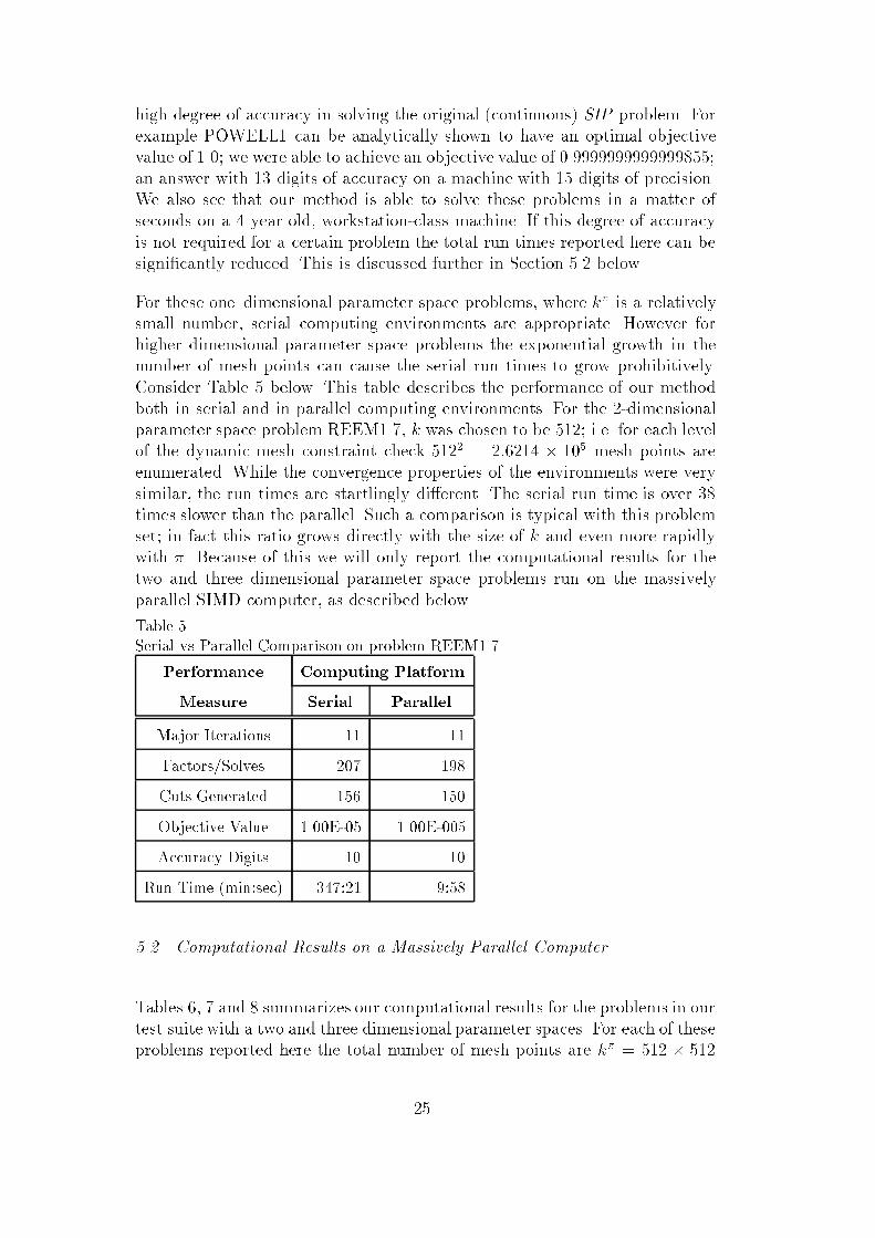
high degree of accuracy in solving the original (continuous) SIP problem. Forexample POWELL1 can be analytically shown to have an optimal objectivevalue of 1.0; we were able to achieve an objective value of 0.9999999999999855;an answer with 13 digits of accuracy on a machine with 15 digits of precision.We also see that our method is able to solve these problems in a matter ofseconds on a 4 year old, workstation-class machine. If this degree of accuracyis not required for a certain problem the total run times reported here can besigni�cantly reduced. This is discussed further in Section 5.2 below.For these one{dimensional parameter space problems, where k� is a relativelysmall number, serial computing environments are appropriate. However forhigher dimensional parameter space problems the exponential growth in thenumber of mesh points can cause the serial run times to grow prohibitively.Consider Table 5 below. This table describes the performance of our methodboth in serial and in parallel computing environments. For the 2-dimensionalparameter space problem REEM1.7, k was chosen to be 512; i.e. for each levelof the dynamic mesh constraint check 5122 = 2:6214 � 105 mesh points areenumerated. While the convergence properties of the environments were verysimilar, the run times are startlingly di�erent. The serial run time is over 38times slower than the parallel. Such a comparison is typical with this problemset; in fact this ratio grows directly with the size of k and even more rapidlywith �. Because of this we will only report the computational results for thetwo and three dimensional parameter space problems run on the massivelyparallel SIMD computer, as described below.Table 5Serial vs Parallel Comparison on problem REEM1.7Performance Computing PlatformMeasure Serial ParallelMajor Iterations 11 11Factors/Solves 207 198Cuts Generated 156 150Objective Value 1.00E-05 1.00E-005Accuracy Digits 10 10Run Time (min:sec) 347:21 9:585.2 Computational Results on a Massively Parallel ComputerTables 6, 7 and 8 summarizes our computational results for the problems in ourtest suite with a two and three dimensional parameter spaces. For each of theseproblems reported here the total number of mesh points are k� = 512 � 51225

and k� = 512 � 512 � 512, respectively. These problems were solved on amassively parallel SIMD machine; MasPar MP2 with 16384 processors. The\time" column in these tables represents CPU time.Table 6Parallel Results { Two Dimensional SIPProblem Major Solves Cuts Objective Value Digits TimeKORT NO3 15 62 40 0.686291501014622 15 5.3POWELL3 16 45 13 0.535891893365735 16 5.1REEM1.2 16 71 30 2.806191129533211E-002 16 35.5REEM1.3 16 133 68 3.473996068787358E-003 16 115.7REEM1.4 14 175 100 6.957447247169803E-004 15 240.3REEM1.5 14 273 156 1.623628352444099E-004 13 588.2REEM1.6 13 192 136 3.964940365252644E-005 11 465.2REEM1.7 11 198 150 1.004179279957140E-005 10 598.7REEM1.8 9 113 85 1.960107200273082E-005 7 393.1REEM1.9 7 122 92 3.993088649984342E-005 7 541.4REEM1.10 7 121 97 6.016127588247359E-005 6 588.5REEM1.15 3 70 61 0.261083371315060 2 657.9Table 7Parallel Results { Two Dimensional SIP (cont)Problem Major Solves Cuts Objective Value Digits TimeREEM2.2 16 76 32 0.177654821833971 16 38.5REEM2.3 15 126 58 3.655363659148542E-002 15 117.2REEM2.4 15 190 118 4.676938687051987E-003 15 256.1REEM2.5 15 240 137 7.385174060762198E-004 14 522.8REEM2.6 11 193 141 7.662267972103893E-005 10 465.8REEM2.7 10 168 131 8.770695228965872E-006 9 451.4REEM2.8 10 183 146 1.056988766754415E-006 9 663.4REEM2.9 6 103 68 3.031789441035943E-004 5 436.9REEM2.10 8 144 114 1.207273990244691E-005 7 768.5Direct computational comparison with other methods is di�cult given thatour method uses a signi�cantly di�erent discretization strategy and and thatwe utilize a parallel computing architecture. Moreover, Reemtsen does notsolve the large problems REEM1.8 through REEM1.15 and REEM2.8 through26

Table 8Parallel Results { Three Dimensional SIPProblem Major Solves Cuts Objective Value Digits TimeREEM3.2 15 125 52 0.152052321303570 14 127.8REEM3.3 16 189 111 3.095701485367659E-002 15 416.0REEM3.4 16 728 550 4.849837980137819E-003 15 2614.2REEM3.5 10 444 317 6.998146322860127E-004 9 3032.0REEM2.10, and does not present computational time, since he used di�erentmachines for di�erent problems, thus a CPU-time comparison would not bevalid [26]. However some comparisons are possible. Because our algorithm doesnot exhaustively enumerate all points in a static mesh, we are able to achievemuch higher local precisions using our discretization scheme within reasonablecomputing time. For example, in the Reemtsen suite of problems (REEM1.�,REEM2.�, and REEM3.�) the �nest grid precisions used were 181 � 181,181 � 181, and 41 � 41 � 41, respectively. We were able to achieve local gridprecisions equivalent to 1:0e9�1:0e9, 1:0e9�1:0e9, and 1:0e9�1:0e9�1:0e9.This has several advantages. It increases the accuracy of the �nal solution (asseen in Tables 2 and 3) while decreasing the probability and magnitude ofarriving at an infeasible solution. All of the solutions reported here are strictlyfeasible up to the local mesh precisions mentioned above. This of course canimprove the con�dence in and quality of the reported results. For example inKORT NO2 a feasibility tolerance of 1:0e� 2 is used to �nd a solution withan objective value of 5:33468728. When this tolerance is improved, we �nd thatthis solution point is infeasible, resulting in an objective value that is overlyoptimistic by 0:16%.Our method also appears to robustly solve the generated convex programmingproblems to a high degree of accuracy. This in turn allows for a higher degreeof precision in the SIP solution. For example, comparing our results with thatof Reemtsen we see that the Chebyshev approximations we �nd are consistentlyslightly better than those found by Reemtsen based on the reported objectivevalues. For the smaller problem instances our method is very stable { typicallyachieving near machine precision in the solution to the discretized problem.However, as the problem sizes grow beyond 50 or 60 variables, we are forcedby numeric stability to stop early. This accounts for the increase in the objectivevalues for such problems as REEM1.9 and REEM1.10.As mentioned above, there is a trade-o� between solution accuracy and the totalwork. For example consider REEM1.7 as shown in Figure 1. This demonstrateshow quickly our algorithm approaches the optimal (approximate) solution dur-ing the initial iterations using very few factorizations (total work). In fact forthis problem a solution was found which had only a 0:1% deviation from the27

�nal solution after the forth major iteration. This solution was found with only29% of the total number of factorizations.102030405060708090100

1 2 3 4 5 6 7 8 9 10 11 12Percentage Major Iteration% of Total Factors 22 2 2 2 2 2 2 2 2 2 2% Distance from Optimality s

s ss s s s s s s s sFig. 1. Progression Toward Optimality: REEM 1.7To do the speedup analysis problem REEM1.2 was selected. It requires ap-proximately thirty seconds to solve using all 16K PEs, which makes solving thesame problems using 1024 PEs within a reasonable amount of time possible.The experiments were run for 1K, 4K, 8K, 12K, and 16K PEs. To help gaugeour implementation's performance, we compute the time at 1024 PEs as thebase from which to plot an ideal speedup for the rest of the data points. Un-derneath this ideal is plotted the observed running time ratios. Our observedratios are within six percent of the ideal.

024681012141618

1024 4096 8192 12288 16384SpeedupThousands Number of Processors544 Seconds 139 Seconds97% Speedup70 Seconds97% Speedup48 Seconds94% Speedup35 Seconds95% Speedup?6

2 2 2 2 2Fig. 2. Speedup Analysis: REEM 1.228

6 ConclusionsIn this paper we have developed a discretization-based cutting plane techniquefor solving convex semi-in�nite programming problems. In doing so we de-veloped a doubly{dynamic discretization technique which was shown to bevery e�ective in practice. Based on our testing across a wide suite of problemsoccurring in the semi-in�nite programming literature we �nd that our methodis both fast and robust.There are several topics for continued research. Currently we generate onlylinear cuts when approximating the true feasible region. One direction of ourcontinuing research is to investigate second order (quadratic) cutting planes.Coupled with quadratic cutting planes we will investigate new ways of addingmulticuts allowing larger, harder problems to be solved. Finally other ways ofdynamically varying the mesh precision shall be explored.AcknowledgementWe gladly thank the PARALLAB, The Institutt for Informatikk at the Uni-versitetet i Bergen, Bergen Norway for providing us with access to their Mas-Par MP-2.The authors are also grateful for the two anonymous referees for their usefulcomments and suggestions that improved the paper substantially.References[1] Bahn, O., J. L. Go�n, J. Ph. Vial, and O. Du Merle, Implementation andbehavior of an interior point cutting plane algorithm for convex programming: anapplication to geometric programming, Discrete Applied Mathematics 49 (1994)3{23.[2] Cheney, E.W. and A. A. Goldstein, Newton's method for convex programmingand tchebyche� approximation, Numerische Mathematik 1 (1959) 243{268.[3] Coope, I.D. and G. A. Watson, A projected lagrangian algorithm for semi{in�niteprogramming,Mathematical Programming 32 (1985) 337{356.[4] Elzinga, J. and T. G. Moore, A central cutting plane algorithm for the convexprogramming problem, Mathematical Programming 8 (1975) 134{145.29

[5] Gribik, P.R., A central{cutting{plane algorithm for semi{in�nite programmingproblems, in: R. Hettich ed., \Lecture Notes in Control and Information Sciences,"Vol. 15. Semi{In�nite Programming (Springer Verlag, New York, 1979) 66{82.[6] Gustafson, S. A. On numerical analysis in semi{in�nite programming, in: R.Hettich, ed., \Lecture Notes in Control and Information Sciences," Vol. 15. Semi{In�nite Programming (Springer Verlag, New York, 1979) 51{65.[7] Gustafson, S. A. and K.O. Kortanek, Numerical solution of a class of semi{in�niteprogramming problems, Naval Research Logistics Quarterly 20 (1973) 477{504.[8] Hettich, R. and K.O. Kortanek Semi{in�nite programming: theory, methods, andapplications, SIAM Review 35 (1991).[9] Den Hertog, D., Interior Point Approach to Linear, Quadratic and ConvexProgramming { Algorithms and Complexity (Kluwer Academic Publisher,Doordrecht, The Netherlands, 1994).[10] Den Hertog, D., F. Jarre, C. Roos, and T. Terlaky, A su�cient condition for self{concordance with application to some classes of structured convex programmingproblems, Mathematical Programming, Series B 69:1 (1995) 75{88 .[11] Den Hertog, D., C. Roos, and T. Terlaky, On the classical logarithmicbarrier method for a class of smooth convex programming problems, Journal ofOptimization Theory and Applications 73:1 (1992) 1{25.[12] Den Hertog, D., C. Roos, and T. Terlaky, A build{up variant of the path{following method for lp, Operations Research Letters 12 (1992) 181{186.[13] Den Hertog, D., C. Roos, and T. Terlaky, Adding and deleting constraints inthe logarithmic barrier method for linear programming problems, in: D. Du andJ. Sun, eds., Advances in Optimization and Approximation, (Kluwer AcademicPublisher, Dordrecht, The Netherlands, 1994) 166{185.[14] Den Hertog, D., J. Kaliski, C. Roos, and T. Terlaky, A logarithmic barrier cuttingplane method for convex programming, Annals of Operations Research 58 (1995)69{98.[15] Jarre, F., The Method of Analytic Centers for Smooth Convex Programs,Dissertation, Institut f�ur Angewandte Mathematik und Statistik, Universit�atW�urzburg, W�urzburg, West{Germany (1989).[16] Kaliski, J. and Y. Ye, A decomposition variant of the potential reductionalgorithm for linear programming,Management Science 39 (1993) 757{776.[17] Kelley, J.E. Jr., The cutting{plane method for solving convex programs, Journalof the Society for Industrial and Applied Mathematics 8 (1960) 703{712.[18] Kortanek, K.O., Semi{in�nite programming duality for order restrictedstatistical inference models, Working Paper, No. 91{18, College of BusinessAdministration, The University of Iowa, Iowa City, Iowa (1991).30

[19] Kortanek, K.O. and H. No, A central cutting plane algorithm for convex semi{in�nite programming problems, SIAM Journal on Optimization 3:4 (1993) 901{918.[20] Kumar, V., A. Grama, A. Gupta, and G. Karypis, Introduction to ParallelComputing. Design and Analysis of Algorithms (The Benjamin/CummingsPublishing Company, Inc., Redwood City CA, 1994).[21] Leon, T. and E. Vercher, New descent rules for solving the linear semi{in�niteprogramming problem, Operations Research Letters 15 (1994) 105{114.[22] Luo, Z. Q., C. Roos, and T. Terlaky, Complexity analysis of logarithmic barrierdecomposition methods for semi-in�nite programming, Research Report (to becompleted), Faculty of Mathematics and Computer Science, Delft University ofTechnology, Delft, The Netherlands (1996).[23] Luo, Z. Q. and Y. Sun, An analytic center based column generation algorithm forconvex quadratic feasibility problems, Research Report, Department of DecisionSciences, National University of Singapore, Singapore (1995).[24] Nesterov,Y.E. and A.S. Nemirovsky, A.S., Interior-Point Polynomial Algorithmsin Convex Programming (SIAM, Philadelphia, USA, 1994).[25] Powell,M. J. D., Log barrier methods for semi{in�nite programming calculations,Numerical Analysis Reports, Department of Applied Mathematics and TheoreticalPhysics, University of Cambridge, DAMTP 1992/NA1 (1992).[26] Reemtsen, R., Some other approximation methods for semi{in�nite optimizationproblems, Journal of Computational and Applied Mathematics 53 (1994) 87{108.

31