Department of informatics

A comparisonbetween two finiteelement methodsfor the solution ofa simplified modelof alloy casting

W. Shen

Research ReportNo. 209ISBN 82-7368-121-1ISSN 0806-3036

December, 1995

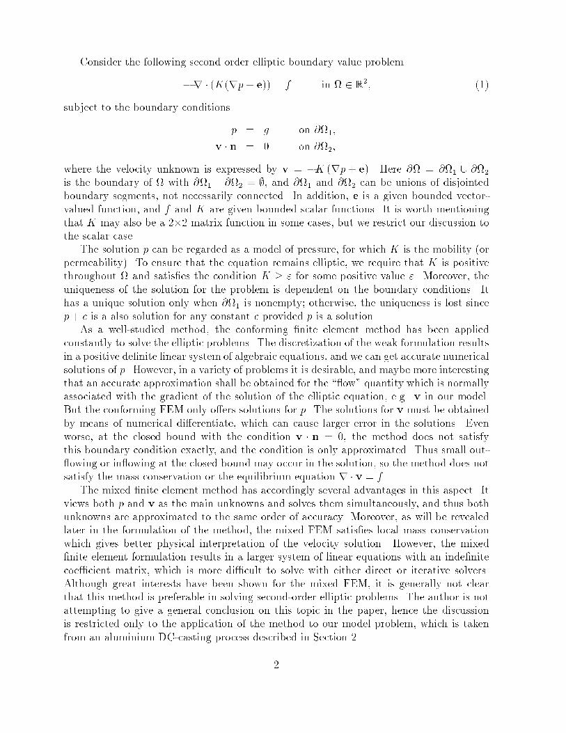
A comparison between two �nite element methods forthe solution of a simpli�ed model of alloy casting �Wen ShenyContents1 Introduction 12 The mathematical model 32.1 The governing equations and the boundary conditions : : : : : : : : : : : : 42.2 Dimensionless equations : : : : : : : : : : : : : : : : : : : : : : : : : : : : : 52.3 Approximation to gl : : : : : : : : : : : : : : : : : : : : : : : : : : : : : : : 63 Finite element methods 74 Numerical experiments 104.1 Poisson equation on a square domain : : : : : : : : : : : : : : : : : : : : : : 104.2 The aluminium DC-casting problem : : : : : : : : : : : : : : : : : : : : : : 115 Conclusions 191 IntroductionThe second-order elliptic boundary value problems consist an important class of problemsin mathematical physics. These equations emerge from the modeling of �ow e.g. in porousmedia and di�erent kinds of reservoir simulations. Therefore, the numerical solutions ofthese problems are of great interests. Various numerical methods approximating second-order elliptic problems have been studied, among them the �nite element methods playan important role. The main purpose of this paper is to investigate two kinds of �niteelement methods, namely the conforming �nite element method and the so-called mixed�nite element method, applied to a model of aluminium casting.�The presented work is supported by The Research Council of Norway through program no. STP.29643,at Section for Applied Mathematics, SINTEF, Oslo, Norway. It is also part of the author's thesis for theCand. Scient. degree.yDepartment of Informatics, University of Oslo, P.O.Box 1080 Blindern, 0316 Olso, Norway, Email:wens@i�.uio.no. 1

Consider the following second order elliptic boundary value problem�r � (K(rp+ e)) = f in 2 R2; (1)subject to the boundary conditionsp = g on @1;v � n = 0 on @2;where the velocity unknown is expressed by v = �K (rp+ e). Here @ = @1 [ @2is the boundary of with @1 \ @2 = ;, and @1 and @2 can be unions of disjointedboundary segments, not necessarily connected. In addition, e is a given bounded vector-valued function, and f and K are given bounded scalar functions. It is worth mentioningthat K may also be a 2�2 matrix function in some cases, but we restrict our discussion tothe scalar case.The solution p can be regarded as a model of pressure, for which K is the mobility (orpermeability). To ensure that the equation remains elliptic, we require that K is positivethroughout and satis�es the condition K � " for some positive value ". Moreover, theuniqueness of the solution for the problem is dependent on the boundary conditions. Ithas a unique solution only when @1 is nonempty; otherwise, the uniqueness is lost sincep+ c is a also solution for any constant c provided p is a solution.As a well-studied method, the conforming �nite element method has been appliedconstantly to solve the elliptic problems. The discretization of the weak formulation resultsin a positive de�nite linear system of algebraic equations, and we can get accurate numericalsolutions of p. However, in a variety of problems it is desirable, and maybe more interestingthat an accurate approximation shall be obtained for the ��ow� quantity which is normallyassociated with the gradient of the solution of the elliptic equation, e.g. v in our model.But the conforming FEM only o�ers solutions for p. The solutions for v must be obtainedby means of numerical di�erentiate, which can cause larger error in the solutions. Evenworse, at the closed bound with the condition v � n = 0, the method does not satisfythis boundary condition exactly, and the condition is only approximated. Thus small out-�owing or in�owing at the closed bound may occur in the solution, so the method does notsatisfy the mass conservation or the equilibrium equation r � v = f .The mixed �nite element method has accordingly several advantages in this aspect. Itviews both p and v as the main unknowns and solves them simultaneously, and thus bothunknowns are approximated to the same order of accuracy. Moreover, as will be revealedlater in the formulation of the method, the mixed FEM satis�es local mass conservationwhich gives better physical interpretation of the velocity solution. However, the mixed�nite element formulation results in a larger system of linear equations with an inde�nitecoe�cient matrix, which is more di�cult to solve with either direct or iterative solvers.Although great interests have been shown for the mixed FEM, it is generally not clearthat this method is preferable in solving second-order elliptic problems. The author is notattempting to give a general conclusion on this topic in the paper, hence the discussionis restricted only to the application of the method to our model problem, which is takenfrom an aluminium DC-casting process described in Section 2.2

The implementation of both the conforming and the mixed FEM has been carried out inDiffpack1. the package of solving PDE using the object-oriented programming languageC++. For the conforming FEM, the corresponding class hierarchy is already establishedin Diffpack, cf. [8]. Based on the implementation for the conforming FEM, The authorimplemented the mixed FEM in a similar style.The paper is organized as follows: In section 2, the aluminium DC-casting surfacesegregation model is described, and the two methods are studied in section 3. Severalcase studies, including the aluminium DC-casting problem, are given in section 4, and wepresent our conclusions at the end of the paper.2 The mathematical modelThe problem de�ned here is motivated from an aluminium direct chill casting process,abbreviated DC-casting. The process ought to be self-explanatory by Figure 1(A): liquidmetal is fed on the top, and cooled �rst by the cold water in the mould, then by the coolingwater �lm on the surface.The melt alloy consists of two components. Aluminium is the major part (95 % ofweight), and the additional metal consists the rest 5% of alloy. The solidi�cation of thealloy takes place in a temperature interval, and thus a region where the solid and liquidphases co-exist appears in space. The region is referred to as the mushy-zone. In thispaper, we are concerned about the pressure and the �ow in the mushy-zone. We quantifythe amount of liquid alloy at any point in the mushy-zone by the volume fraction of liquidgl. The value of gl varies from 0 to 1, by which gl = 0 means solid, and gl = 1 indicatesliquid. In this model, we assume that the distribution of gl is known.2The quality of the cast alloy is dependent on the distribution of the alloy element, andonly the alloy which has the 5% alloy element evenly distributed possesses the satisfactoryproperties. Unfortunately, this 5% component might become unevenly distributed in spaceduring the solidi�cation. A non-uniform spatial distribution of this quantity is calledmacro-segregation, which has bad e�ect on the quality of the product. In our model,metallostatic overpressure causes convection of species-rich melt towards the surface ofthe cast aluminium. This leads to the so-called surface segregation. As the temperaturedrops, the density of the alloy increases, which causes the volume to decrease. Due tothis shrinking e�ect during solidi�cation, an air gap appears between the lower part of themould and the mushy-zone, and the liquid will �ow out and create a surface layer. This�ow phenomenon is referred to as exudation, cf. [5, page 252]. The surface layer beingformed by the exuding inter-dendritic liquid is highly enriched in alloy element, and mustbe removed before the aluminium alloy is processed further. In industry this operation isvery expensive. Therefore, the area close to this air gap is referred to as the critical region1The development of Diffpack is supported by The Research Council of Norway (NFR) through theresearch program no. STP 28402: Toolkits in Industrial Mathematics at SINTEF2Actually, the distribution of gl is also an unknown which is governed by an equation of energy con-servation. Such a complete model in one space dimension is studied in [6]. Our approximation of gl inSection 2.3 is based on their results of the one dimension case.3

of the problem, and the velocity solution in this region is of particular interests.2.1 The governing equations and the boundary conditionsWe study a 2D�model of the mushy-zone in the DC-casting process that reaches a sta-tionary state, i.e., all the parameters are independent of time. Since the intersection issymmetric in the stationary state (cf. Figure 1(A)), we only need to study half of themushy-zone. The solution domain for the equations is indicated in Figure 1(B). The pres-sure and velocity �elds are the outputs of our model, and the velocity solution is of specialinterests because it o�ers access to other important parameters for the problem.(A) (B)Secondary

Feeding of liquid metal

Soldified

Liquid melt

Mushy zone

Casting direction

Hot top

MouldWater

water filmCooling

Starting block

Primary water cooling

water cooling

1

4

L

SH

Γ

2

Γ

2

33Γ

2Γ

n

Γ5

CH

L

L

x 1

x

Figure 1: The aluminium DC-casting process. (A): The process. (B): The solution domain. The model is based on the general volume averaged conservation equations. We assumethat the density of liquid aluminium and the casting velocity are constants. Conservationof mass in liquid gives @@x1(glu1) + @@x2(glu2) = 0; (2)where gl is the volume fraction of liquid, and u = (u1; u2) is the intrinsic velocity. Inaddition, Darcy's law gives gl�K u1+ @p@x1 = 0; (3)gl�K u2+ @p@x2 + �g = 0; (4)4

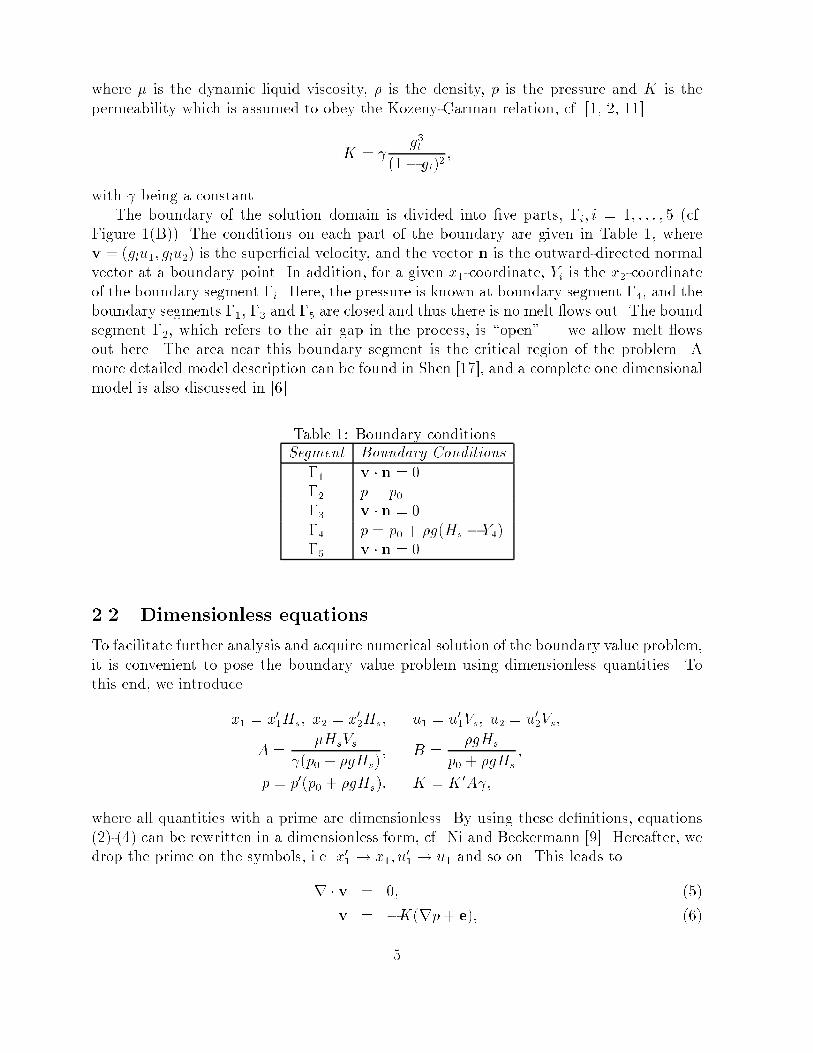
where � is the dynamic liquid viscosity, � is the density, p is the pressure and K is thepermeability which is assumed to obey the Kozeny-Carman relation, cf. [1, 2, 11]K = g3l(1� gl)2 ;with being a constant.The boundary of the solution domain is divided into �ve parts, �i; i = 1; : : : ; 5 (cf.Figure 1(B)). The conditions on each part of the boundary are given in Table 1, wherev = (glu1; glu2) is the super�cial velocity, and the vector n is the outward-directed normalvector at a boundary point. In addition, for a given x1-coordinate, Yi is the x2-coordinateof the boundary segment �i. Here, the pressure is known at boundary segment �4, and theboundary segments �1, �3 and �5 are closed and thus there is no melt �ows out. The boundsegment �2, which refers to the air gap in the process, is �open� � we allow melt �owsout here. The area near this boundary segment is the critical region of the problem. Amore detailed model description can be found in Shen [17], and a complete one dimensionalmodel is also discussed in [6].Table 1: Boundary conditions.Segment Boundary Conditions�1 v � n = 0�2 p = p0�3 v � n = 0�4 p = p0 + �g(Hs � Y4)�5 v � n = 02.2 Dimensionless equationsTo facilitate further analysis and acquire numerical solution of the boundary value problem,it is convenient to pose the boundary value problem using dimensionless quantities. Tothis end, we introducex1 = x01Hs; x2 = x02Hs; u1 = u01Vs; u2 = u02Vs;A = �HsVs (p0 + �gHs); B = �gHsp0 + �gHs ;p = p0(p0 + �gHs); K =K 0A ;where all quantities with a prime are dimensionless. By using these de�nitions, equations(2)-(4) can be rewritten in a dimensionless form, cf. Ni and Beckermann [9]. Hereafter, wedrop the prime on the symbols, i.e. x01 ! x1; u01 ! u1 and so on. This leads tor � v = 0; (5)v = �K(rp+ e); (6)5

where v = (glu1; glu2) and e = (0; B)T . By eliminating v, we obtain equation (1) withf � 0, @1 = �2 [ �4 and @2 = �1 [ �3 [ �5. Hence, the dimensionless permeabilitybecomes K(gl) = g3lA(1� gl)2 , and the corresponding boundary conditions are summarizedin Table 2. By choosing the material and process parameters as listed in Table 3, we obtainA = 3:3121113 and B = 0:860155:Table 2: Boundary conditions for the dimensionless equations.Segment Boundary conditions�1 v � n = 0�2 p = 0�3 v � n = 0�4 p = 1�BY4�5 v � n = 0Table 3: The material and the process parameters.Parameter Value� 2385 kg/m3� 1:2 � 10�3 Ns/m2 10�11 m2p0 1900 PaVs 7:5 � 10�4 m/sg 9:8 m/s2L 0:24 mHc 0:1028 mHs 0:5 mL2 0:0469 mL3 0:0611 m2.3 Approximation to glBased on the results for the complete one dimensional model in [6], we assume gl to be alinear function which takes value "1 at �1 and (1� "2) at �4, i.e.,gl(x1; x2) = 1� "2 � 1� "1 � "2Y4(x1)� Y1(x1)(Y4(x1)� x2):Here, two small positive constants "1 and "2 are used in order to obtain a well-posedvariational problem according to the Lax-Milgram Theorem, cf. Johnson [7]. Di�erentchoices of ("1, "2) will be used to investigate the feature of the numerical solutions whenthe mobility function K is close to singular. 6

3 Finite element methodsIn this section we describe two �nite element methods by giving the weak formulations ofthe general elliptic equation (1). We also give the error estimates and mention possiblesolvers for the linear system of algebraic equations for the two methods.In order to give the proper variational problem, we need some basic notations. LetH1() be the standard Sobolev space which is de�ned asH1() = np : p 2 L2(); rp 2 �L2()�no ;and the subspace H10() = np : p 2 H1(); p = 0 on @1o ;with the norm kpkH1() = �kpk20; + krpk20;�12 ;where n is the number of space dimensions, andkpk20; = Z jpj2 dx:We also introduce the spaceH(div;) = nv : v 2 (L2())n;r � v 2 L2()o ;and the subspace H0(div;) = fu 2 H(div;); u � n = 0 on @2g ;together with the norm k v kH(div;)= �k v k20; + k r � v k20;�12 :For the conforming FEM, the variational problem of (1), which is also referred to asthe weak formulation, reads: Find p � pg 2 H10() such thatZ(Krp) � rq dx = Z fq dx� Z(Ke) � rq dx 8q 2 H10(); (7)where pg 2 H1() and pg = g on @1. Existence of a unique weak solution of the formu-lation follows from the Lax-Milgram Theorem, cf. Johnson [7].By de�ning the �nite-dimensional subspaces asVh() � H1(); Vh;0() � H10();we discretize the formulation (7) as: Find ph � ph;g 2 Vh;0() such thatZ(Krph) � rq dx = Z fq dx� Z(Ke) � rq dx 8q 2 Vh;0(); (8)7

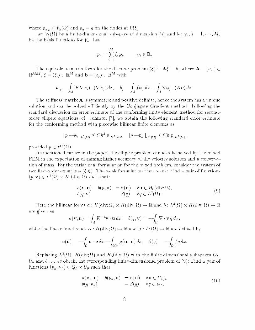
where ph;g 2 Vh() and pg = g on the nodes at @1.Let Vh() be a �nite-dimensional subspace of dimension M , and let 'i, i = 1; � � � ;M ,be the basis functions for Vh. Letph = MXi=1 �i'i; �i 2 R:The equivalent matrix form for the discrete problem (8) is A� = b, where A = (aij) 2RM;M , � = (�i) 2 RM and b = (bj) 2 RM withaij = Z(Kr'i) � (r'j)dx; bj = Z f'j dx� Zr'j � (Ke)dx:The sti�ness matrixA is symmetric and positive de�nite, hence the system has a uniquesolution and can be solved e�ciently by the Conjugate Gradient method. Following thestandard discussion on error estimate of the conforming �nite element method for second-order elliptic equations, cf. Johnson [7], we obtain the following standard error estimatefor the conforming method with piecewise bilinear �nite elements askp� phkL2() � Ch2jpjH2(); kp� phkH1() � ChjpjH2();provided p 2 H2().As mentioned earlier in the paper, the elliptic problem can also be solved by the mixedFEM in the expectation of gaining higher accuracy of the velocity solution and a conserva-tion of mass. For the variational formulation for the mixed problem, consider the system oftwo �rst-order equations (5-6). The weak formulation then reads: Find a pair of functions(p;v) 2 L2()�H0(div;) such that:a(v;u) + b(p;u) = �(u) 8u 2 H0(div;);b(q;v) = �(q) 8q 2 L2(): (9)Here the bilinear forms a :H(div;)�H(div;) 7! R and b : L2()�H(div;) 7! Rare given as a(v;u) = ZK�1v � u dx; b(q;v) = � Zr � v q dx;while the linear functionals � :H(div;) 7! R and � : L2() 7! R are de�ned by�(u) = � Z u � edx� Z@1 g(u � n)ds; �(q) = � Z fq dx:Replacing L2(), H(div;) and H0(div;) with the �nite-dimensional subspaces Qh,Uh and Uh;0, we obtain the corresponding �nite-dimensional problem of (9): Find a pair offunctions (ph;vh) 2 Qh � U0 such thata(vh;u) + b(ph;u) = �(u) 8u 2 Uh;0;b(q;vh) = �(q) 8q 2 Qh: (10)8

The choice of the �nite-dimensional subspaces Qh and Uh is of great importance forobtaining a stable and accurate solution. The choice is also di�cult to make because manycombinations will not produce appropriate results. Moreover, the stability and accuracydemands stay in con�ict in some sense, thus one has to �nd a reasonable compromise. Thecrucial inequality that will guarantee the stability of the mixed method is called Babuska-Brezzi condition which reads: There is a positive constant c independent of h such that forall q 2 Qh supv2Uh b(q;v)kvkH(div;) � ckqkL2():Roughly speaking, for a given pressure subspace Qh, the velocity subspace Uh must belarge enough, and the challenge is how to choose Uh nearly as small as possible.The lowest-order mixed �nite element, which is also referred to as the lowest orderRaviart-Thomas element (cf. [12]), is used in this paper. We use piecewise constant trialfunctions for the pressure p, and for the velocity v we use the trial functions whose di-vergence are piecewise constant. This subspace is known to satisfy the Babuska-Brezzicondition. The analysis of Brezzi [3], Raviart and Thomas [12] and Falk and Osborn [4]yields the following error estimate for the mixed FEM,kp� phkL2() � Ch; kv� vhkH(div;) � Ch;where C is constant depending upon the smoothness of p and v and the solution domain.We refer to [3, 12, 13, 14, 18, 19] for more detailed discussion on the mixed method andalternative choices of mixed �nite elements.One attractive aspect of the mixedmethod is related to the super-convergence character,i.e., the mixed �nite element method has super-convergence at the centroid of the element.To be precise, when discrete norms such as l1- and l2-norm are used, the convergence ratesfor both p and v are of order 2 if the lowest-order Raviart-Thomas elements are used.Let f�ignpi=1 and f ignvi=1 = f( 1;i; 2;i)gnvi=1 denote the bases for the subspaces Qh (pres-sure) and Uh (velocity), respectively. The discrete problem (10) can be written in matrixform as M� �B� = cBT� = dwhere M = (mij), B = (bij), c = (cj), d = (dj), withmij = a( i; j); bij = b(�i; j); cj = �( j); dj = �(�j);and � and � are the coordinates for ph and vh. It is not di�cult to prove that the coe�cientmatrix of this system is symmetric, nonsingular and inde�nite. Such system can be solvediteratively using e.g. the minimum residual method proposed by Piage and Saunders[10], with a suitable preconditioner, e.g., the preconditioned iterative method for inde�nitelinear systems corresponding to certain saddle-point problems suggested by Rusten andWinther [16], or the domain decomposition preconditioners by the same authors [15]. For9

the direct solver, it is not clear in general that Gaussian elimination without pivoting willwork for this kind of system. But our numerical experiments shows this works �ne for ourmodel. In this case, we should renumber the nodes such that the bandwidth of the matrixis minimized. It is also important to mention that there exist di�erent kinds of �hybrid�methods, and the mixed method discussed above is only one of them.To this end, we can summary the comparison between the two �nite methods, which islisted in Table 4.Table 4: Summary of the comparison of the conforming and the mixed FEM.The conforming FEM The mixed FEMEasy to implement F Hard to implement HEasy to solve the linear system F Hard to solve the linear system HAccurate pressure solution F Accurate pressure solution FNo direct access to v H Direct access to v FLower accuracy in v H Higher accuracy in v FNo local mass conservation H Local mass conservation FNot satisfy the equilibrium H Satisfy the equilibrium Fequation r � v = f equation r � v = fF: AdvantageH: Disadvantage4 Numerical experimentsIn this section, we continue our study of the conforming and the mixed FEM with somenumerical experiments. The Poisson equation is solved before we present the solution ofthe aluminium DC-casting problem.4.1 Poisson equation on a square domainBefore we solve the pressure equation of the aluminium DC-casting problem, we study asimple case of the Poisson equation de�ned on a unit square domain = [0;1]� [0; 1]:��p = 2�2 sin(�x1) sin(�x2) in ;associated with the boundary conditionsp = 0 on @:It is easy to prove that the analytical solution of p isp = sin(�x1) sin(�x2);and v = �rp isv1 = �� cos(�x1) sin(�x2) and v2 = �� sin(�x1) cos(�x2):10

Actually, this is just a special case of our general problemwith f = 2�2 sin(�x1) sin(�x2),K � 1 and the corresponding boundary conditions. This problem is solved with both theconforming and the mixed FEM. The estimated rates of convergence for both methodsand for the di�erences between the numerical solutions of the two methods are listed inTable 5.Note that di�erent norms are used in measuring the errors, among those L2- andH(div;)-norms are continuous norms, while l2- and l1-norms are discrete norms whosediscrete points are taken at the centroid of each element. The rate of convergence a iscomputed by a = log(h1=h2)= log(e1=e2);where h1 and h2 are two grid size, and e1 and e2 are the corresponding errors.The results �t the error estimates from previous section very well. For the conformingFEM solutions, we obtain 2 as the rate of convergence for p in L2-norm, and 1 for v(whichis the same rate for pressure solution in H1-norm). The mixed FEM solutions give 1 asthe rate of convergence for both p and v in L2-norm. The super-convergence characteristicof the mixed FEM solution is clearly demonstrated in this case: the rates of convergencein discrete norms are 2. We also see that the errors between two numerical solution indi�erent norms converge towards zero at a rate 1(resp. 2) in continuous(resp. discrete)norms. Table 5: The estimated rates of convergence for the Poisson equation.pressure solutions velocity solutionsnorm L2 l2 l1 H(div;) L2 l2 l1conforming 1.9995 1.9590 2.0021 � 0.9994 2.0007 1.9903mixed 0.9986 1.9979 1.9875 0.9994 0.9994 2.0007 1.9903di�erence 0.9985 1.9997 1.9756 � 0.9999 2.0047 1.97474.2 The aluminium DC-casting problemThe aluminium DC-casting problem is solved with both conforming and mixed FEM im-plemented in Diffpack. The results are presented in this section with graphs and tables.In order to understand the results better, we �rst describe some basic implementationconcepts.The mesh grid is generated by the preprocessor in Diffpack with a conventional tech-nique: First, the domain is divided into several large elements, so-called super elements.Second, the preprocessor discretize each super element according to the given partitionrequirements. Third, these grid patches are combined into a global �nite element grid.In our aluminium problem, the solution domain is divided into 9 super elements, i.e., if4x4 partition is used in each super element, we have in total 4x4x9=144 �nite elementsin the grid. An example of such a mesh grid is included in Figure 4.2(A), in which thethick lines sketch the super elements, and the dotted lines show the partition in each superelement. Note that the partitions mentioned later in this subsection mean the partition11

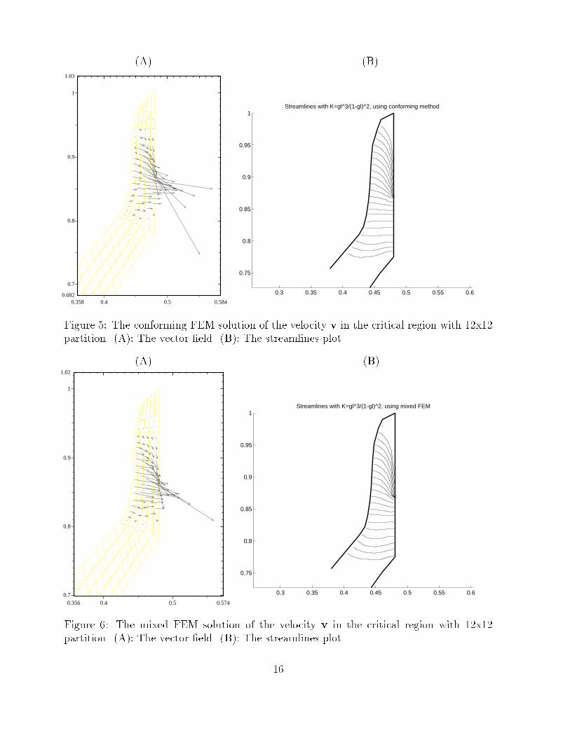
in each super element. In other words, the whole domain is always divided into 9 superelement.We use quadrilateral �nite elements and the Gauss-Legendre quadrature as the numeri-cal integration scheme. For small systems (i.e., partition in each super element is not largerthan 8x8), we use Gaussian elimination without pivoting, and for larger systems we useiterative methods. The linear system for the conforming FEM is symmetric and positivede�nite, so the conjugate gradient method is our natural choice, and the preconditioningtype being used is ILU (Incomplete LU factorization). For the mixed FEM, Gaussian elim-ination without pivoting is proven to be su�cient for small systems, while large systemscan be solved iteratively by e.g. the minimum residual method.Graphical results: The problem is solved with di�erent choices of ("1, "2) values thatare close to 0. Notice that "1 = 0 indicates K = 0 when gl = 0, while "2 = 0 cause K goestowards in�nite if gl = 1, thus the mathematical problem is no longer well-posed. However,no di�erences can be observed by eyes between the graphs that are obtained by di�erent("1, "2) values between (0.1,0.1) and (0,0). Hence, the graphical results presented later inthis subsection uses "1 = "2 = 0 if not speci�ed. Following is a list of the plots with somecomments:� The contourline-plot for the volume fraction of the liquid aluminium gl is shown inFigure 4.2(B). This is the input argument of our problem, which is given to be 1 on�4 and 0 on �1.� The pressure solutions are plotted in Figures 3 and 4. Plot 3(A) is the contourline-plotof the conforming FEM solution, with a enlargement of the critical region in plot 3(B).The similar plots for the mixed solution of pressure can be found in plots 4(A)and 4(B). Since piecewise constant elements are used for the pressure solutions, itis inconvenient to plot the contourlines, so we give the shaded plots. When thegrid becomes �ner, we can observe that the solution from the mixed FEM becomesanalogous to the one from the conforming FEM.� In Figures 5 and 6 we give the velocity solutions. Since the velocity solutions van-ish outside the critical region, we only plot the solutions in the critical region. Theconforming FEM velocity solutions are obtained by taking numerical gradient of thescalar pressure solutions, and they are included in plot 5(A) with a streamline plotin 5(B). The mixed FEM velocity solutions is solved directly in the weak formula-tion, and they are given in plots 6(A)(vector �eld) and 6(B)(streamline plot). Thestreamline plot shows the movement of aluminium particles, and since the velocity�eld is stationary, the streamline is the same as the particlepath. Note that the �-nite element grid is also displayed in the plots and the arrows are originated in thecentroid of each element. The length of the arrow indicates the scale of speed. Wenotice that there is di�erence between the solutions of the two methods with a coarsegrid, but the di�erence becomes smaller for �ner grids.12

� As mentioned before, the horizontal component of the velocity solutions close to thebound segments �2 and �3 is of particular interest. Thus, we plot this parameter inFigure 7, where plot (A) is for the conforming FEM and plot (B) is for the mixedFEM. The conforming FEM solution gives non-zero value at bound �3 where isclosed. This is physically incorrect and causes the void of the conservation of mass.This is considered to be the main disadvantage of the method. The mixed FEMgives piecewise constant horizontal velocity component, and the discontinuity in thesolution at the point that joints �2 and �3 is exactly approximated. One can actuallycalculate the amount of out-�owing melt by integrating this horizontal velocity overbound �2, and such a calculation shows that the mixed FEM solution gives higheramount of out-�owing.It is obvious that the two methods give close results. Here we give some physicalremarks about the pressure and velocity solutions of the model:� The solution for the pressure p shows that in the lower part of the domain, p variesslowly and smoothly, with almost horizontal contour lines. But in the critical region,p shows rapid variation. Especially at the part which is very close to �2 where thealuminium is supposed to run out, we �nd almost vertical contour lines.� The relation between the velocity v and the pressure p is given by v = �K(rp+ e):As we see from the solution for the pressure, p varies vertically and smoothly inthe lower part of the domain. Since the e�ect of rp is totally cancelled out by theconstant vector e in this area, the corresponding solution v is zero. In contrast,p varies quickly in the critical region, which means the corresponding velocity isno longer zero. A closer look at the region near the boundary �2 reveals that thedirection of the velocity is almost horizontal, which is indicated by the horizontal-varying pressure solution. The plots of the streamlines in the critical region show thesituation more clearly.Tabular results: Our estimate of the rates of convergence is restricted to the conformingFEM3 for the pressure and the velocity solutions with di�erent ("1, "2) values, which islisted in Table 6 and 7. For the pressure solution, we use the standard H1- and L2-norm,and for the velocity solution, we study also the standard L2-norm. In addition, since thevelocity is decided by v = �K(rp+ e); we introduce the alternative normkpk �H1() = �jjpjj2L2() + jjKrpjj2L2()�12 :This norm is sensitive to the mobility function �, and it is easy to prove that the normis actually equivalent to the standard L2-norm for the velocity solution. From these tables,we observe that the rates of convergence for the pressure solution varies very little as ("1,"2) value reduces towards zero. However, the rates of convergence for the velocity solutionare very sensitive to the ("1, "2) value. When ("1, "2) value is too small, e.g., "1 = "2 = 0:01in our case, the errors do not decrease when the grid becomes �ner.3Due to lack of e�cient iterative linear solvers for inde�nite systems in Diffpack, similar estimate forthe mixed FEM is limited only to relative small systems.13

(A) (B)0 0.1 0.2 0.3 0.4 0.48

0

1

mesh grid

X−Axis

Y−

Axi

s

0 0.1 0.2 0.3 0.4 0.480

1

Finite element scalar field for Gl

X−Axis

Y−

Axi

s

0.06

26

0.06

26

0.06

26

0.18

8

0.18

8

0.18

8

0.313

0.31

3

0.31

3

0.31

3

0.43

8

0.43

8

0.43

8

0.56

2

0.56

2

0.56

2

0.56

2

0.68

7

0.68

7

0.68

7

0.81

2

0.81

2

0.81

2

0.937

0.93

7

0.93

7

0.93

7

0

1

Figure 2: (A): An example of the mesh grid generated by super element preprocessor with4x4 partition in each super element. (B): Plot of the volume fraction liquid aluminium Gl.14

(A) (B)0 0.1 0.2 0.3 0.4 0.48

0

1

Conforming FEM solution of Pressure

X−Axis

Y−

Axi

s

0.1

0.14

0.22

0.42

0.62

0.7

0.78

0.82

0.86

0.9

0.41 0.42 0.43 0.44 0.45 0.46 0.47 0.48

0.8

0.9

0.744

0.931

X−Axis

0.02

0.02

0.060.06

0.1

0.10.14

0.14

0.18

0.18

0.22

0.22

0.22

0.26

0.26

0.3

0.34

0.8

0.9

0.744

0.931

Figure 3: The conforming FEM solution of the pressure P . (A): The whole solutionsdomain. (B): An enlargement of the critical region.(A) (B)0 0.1 0.2 0.3 0.4 0.48

0

1

0.0381

0.133

0.227

0.322

0.417

0.511

0.606

0.7

0.795

0.89

0.984

0

1

0.4 0.42 0.44 0.46 0.48

0.8

0.9

1

0.750.0381

0.133

0.227

0.322

0.417

0.511

0.606

0.7

0.795

0.89

0.984

0.8

0.9

1

0.75Figure 4: The mixed FEM solution of the pressure P . (A): The whole solutions domain.(B): An enlargement of the critical region. 15

(A) (B)0.4 0.50.358 0.584

0.7

0.8

0.9

1

0.682

1.03

0.7

0.8

0.9

1

0.682

1.03

0.3 0.35 0.4 0.45 0.5 0.55 0.6

0.75

0.8

0.85

0.9

0.95

1Streamlines with K=gl^3/(1-gl)^2, using conforming method

Figure 5: The conforming FEM solution of the velocity v in the critical region with 12x12partition. (A): The vector �eld. (B): The streamlines plot.(A) (B)0.4 0.50.356 0.574

0.7

0.8

0.9

1

1.02

0.7

0.8

0.9

1

1.02

0.3 0.35 0.4 0.45 0.5 0.55 0.6

0.75

0.8

0.85

0.9

0.95

1Streamlines with K=gl^3/(1-gl)^2, using mixed FEM

Figure 6: The mixed FEM solution of the velocity v in the critical region with 12x12partition. (A): The vector �eld. (B): The streamlines plot.16

Table 6: The errors and the rates of convergence for p, the conforming FEM.partitions k�e(p)kH1() rate �a k�e(p)kL2() rate �a"1 = "2 = 0:1:(1x1)�(2x2) 4.8382e-01 � 6.4126e-03 �(2x2)�(4x4) 2.7462e-01 0.8170 1.5895e-03 2.0123(4x4)�(8x8) 1.5315e-01 0.8425 5.7771e-04 1.4602(8x8)�(16x16) 8.8667e-02 0.7885 2.0493e-04 1.4952(16x16)�(32x32) 4.9033e-02 0.8546 7.6539e-05 1.4209"1 = "2 = 0:01:(1x1)�(2x2) 5.0392e-01 � 6.6579e-03 �(2x2)�(4x4) 3.0718e-01 0.7141 2.1239e-03 1.6484(4x4)�(8x8) 1.8191e-01 0.7559 9.6634e-04 1.1361(8x8)�(16x16) 1.1161e-01 0.7048 4.1728e-04 1.2115(16x16)�(32x32) 6.5716e-02 0.7641 1.6619e-04 1.3282"1 = "2 = 0:001:(1x1)�(2x2) 5.0492e-01 � 6.6751e-03 �(2x2)�(4x4) 3.0341e-01 0.7348 2.1945e-03 1.6049(4x4)�(8x8) 1.8712e-01 0.6973 1.0376e-03 1.0806(8x8)�(16x16) 1.0985e-01 0.7684 4.7991e-04 1.1124(16x16)�(32x32) 6.6759e-02 0.7185 2.1378e-04 1.1666"1 = 0;"2 = 0:01:(1x1)�(2x2) 5.0442e-01 � 6.6636e-03 �(2x2)�(4x4) 3.0356e-01 0.7326 2.1989e-03 1.5995(4x4)�(8x8) 1.8778e-01 0.6929 1.0448e-03 1.0736(8x8)�(16x16) 1.1073e-01 0.7620 4.8710e-04 1.1009(16x16)�(32x32) 6.7703e-02 0.7098 2.2031e-04 1.1447"1 = 0:01; "2 = 0:(1x1)�(2x2) 5.0456e-01 � 6.6719e-03 �(2x2)�(4x4) 3.0778e-01 0.7131 2.1280e-03 1.6486(4x4)�(8x8) 1.8236e-01 0.7551 9.6781e-04 1.1367(8x8)�(16x16) 1.1190e-01 0.7046 4.1818e-04 1.2106(16x16)�(32x32) 6.5896e-02 0.7639 1.6669e-04 1.3270"1 = 0;"2 = 0:(1x1)�(2x2) 5.0502e-01 � 6.6770e-03 �(2x2)�(4x4) 3.0409e-01 0.7318 2.2022e-03 1.6003(4x4)�(8x8) 1.8812e-01 0.6928 1.0455e-03 1.0748(8x8)�(16x16) 1.1092e-01 0.7621 4.8739e-04 1.1010(16x16)�(32x32) 6.7800e-02 0.7102 2.2043e-04 1.144817

Table 7: The errors and the rates of convergence for v, the conforming FEMpartitions k�e(p)k �H1() rate �a k�e(v)kL2() rate �a"1 = "2 = 0:1:(1x1)�(2x2) 7.55589e-01 � 7.55562e-01 �(2x2)�(4x4) 3.33723e-02 4.5009 3.33345e-02 4.5025(4x4)�(8x8) 1.51326e-02 1.1410 1.51231e-02 1.1403(8x8)�(16x16) 9.40193e-03 0.6866 9.40015e-03 0.6860(16x16)�(32x32) 5.34516e-03 0.8147 5.34478e-03 0.8146"1 = "2 = 0:01:(1x1)�(2x2) 2.74719e+00 � 2.74719e+00 �(2x2)�(4x4) 4.12368e-02 6.0579 4.11911e-02 6.0595(4x4)�(8x8) 1.74787e-02 1.2383 1.74637e-02 1.2380(8x8)�(16x16) 1.64148e-02 0.0906 1.64123e-02 0.0896(16x16)�(32x32) 1.21511e-02 0.4339 1.21507e-02 0.4337"1 = "2 = 0:001:(1x1)�(2x2) 3.55862e+00 � 3.55861e+00 �(2x2)�(4x4) 4.27928e-02 6.3778 4.27484e-02 6.3793(4x4)�(8x8) 1.82186e-02 1.2320 1.82025e-02 1.2317(8x8)�(16x16) 2.01453e-02 -0.1450 2.01430e-02 -0.1461(16x16)�(32x32) 1.77009e-02 0.1866 1.77007e-02 0.1865"1 = 0; "2 = 0:01:(1x1)�(2x2) 3.91263e+00 � 3.91262e+00 �(2x2)�(4x4) 4.52028e-02 6.4356 4.51609e-02 6.4369(4x4)�(8x8) 1.94547e-02 1.2163 1.94412e-02 1.2160(8x8)�(16x16) 2.22057e-02 -0.1908 2.22038e-02 -0.1917(16x16)�(32x32) 1.99853e-02 0.1520 1.99850e-02 0.1519"1 = 0:01; "2 = 0:(1x1)�(2x2) 2.68980e+00 � 2.68979e+00 �(2x2)�(4x4) 3.92563e-02 6.0984 3.92077e-02 6.1002(4x4)�(8x8) 1.64941e-02 1.2510 1.64760e-02 1.2508(8x8)�(16x16) 1.53784e-02 0.1010 1.53754e-02 0.0997(16x16)�(32x32) 1.14581e-02 0.4245 1.14577e-02 0.4243"1 = 0; "2 = 0:(1x1)�(2x2) 3.82484e+00 � 3.82484e+00 �(2x2)�(4x4) 4.30092e-02 6.4746 4.29647e-02 6.4761(4x4)�(8x8) 1.83201e-02 1.2312 1.83038e-02 1.2310(8x8)�(16x16) 2.07214e-02 -0.1777 2.07191e-02 -0.1788(16x16)�(32x32) 1.87487e-02 0.1443 1.87485e-02 0.144218

(A) (B)0.75 0.8 0.85 0.9 0.95 1

−1

−0.5

0

0.5

1

1.5

2

2.5

3

3.5conforming FEM, e1=e2=0.0, 8x8 partition

0.75 0.8 0.85 0.9 0.95 1−0.5

0

0.5

1

1.5

2Mixed FEM, e1=e2=0, 8x8 partition

Figure 7: The horizontal component of velocity at �2 and �3. (A): Conforming FEM. (B):Mixed FEM.5 ConclusionsWe claim that both the conforming and the mixed �nite element methods behave wellapproximating the general second-order elliptic boundary value problems. Applied to thealuminium DC-casting model problem, both methods give good results. The conformingmethod results in a symmetric positive de�nite coe�cient matrix, and gives accurate pres-sure solution. But the velocity solution can only be obtained by taking numerical gradientof the pressure solution, and thus loses accuracy. This can be regarded as the main disad-vantage of the method. In many model problems, v has important physical meanings, andis often more interesting. Our DC-casting model is an example. Sometimes, one wouldrather have a more accurate velocity solution. Therefore, the mixed method is superiorin this aspect. The mixed pressure and velocity solutions have the same order of accu-racy. One drawback of the mixed method is that it is trickier to implement, and it resultsin larger linear inde�nite system of equations which is more di�cult to solve. So if onlythe pressure is interesting, one should always use the optimal conforming method. Whenaccurate velocity solution is desired, one should try the mixed method.Acknowledgment: The author wants to thank her supervisor Aslak Tveito at Institutefor Informatics, University of Oslo for his encouragement and guiding. She also thanksTorgeir Rusten at Section for Applied Mathematics, SINTEF for carefully reading thisscript and giving lots of corrections.References[1] S. Asai and I. Muchi, Theoretical analysis and model experiments on the formationmechanism of channeltype segregation, Trans. Iron Steel Inst. Japan, 18:90-98, 1978.19

[2] W.D. Bennon and F.P. Incropera, A continuum model for momentum, heatand species transport in binary solid-liquid phase change systems � II. application tosolidi�cation in a rectangular cavity, International Journal of Heat and Mass Transfer,30(10): 2171-2187, 1987.[3] F. Brezzi, On the existence, uniqueness and approximation of saddle-point problemsarising from Lagrangian multipliers, RAIRO Numer. Anal. 8, (1974), pp. 129�151.[4] R. Falk and J. Osborn, Error estimates for mixed methods, R.A.I.R.O., (1980),pp. 249�277.[5] M. C. Flemings, Solidi�cation processing, McGraw-Hill, 1974.[6] E. Haug, A. Mo and H. Thevik, Macrosegregation near a cast surface caused byexudation and solidi�cation shrinkage, Preprint, International Journal of Heat andMass Transfer.[7] C. Johnson, Numerical solution of partial di�erential equations by the �nite elementmethod, Claes Johnson and Studentlitteratur, Lund, 1987.[8] H. P. Langtangen, Di�pack: Software for partial di�erential equations, (To appearin the proceedings of OONSKI'94), (1994).[9] J. Ni and C. Beckermann, A volume-averaged two-phase model for transport phe-nomena during solidi�cation, Metallurgical Transactions, 22B, (1991), pp. 349�361.[10] C. C. Paige and M. A. Saunders, Solution of sparse inde�nite systems of linearequations, SIAM J. Numer. Anal., 12 (1975), pp. 617�629.[11] D.R. Poirier, Permeability for �ow of interdendritic liquid in columnar-dendriticalloys, Metallurgical Transaction, 18B: 245-255, 1987.[12] P. A. Raviart and J. M. Thomas, A mixed �nite element method for 2-nd orderelliptic problems, in Mathematical Aspects of Finite Element Methods, Lecture Notesin Mathematics 606, I. Galligani and E. Magenes, eds.,, (1977), pp. 295�315.[13] J. E. Roberts and J. M. Thomas, Mixed and hybrid method, in Handbook ofNumerical Analysis, Vol. II, P. G. Ciarlet and J. L. Lions, eds., (1991).[14] T. F. Russel and M. F. Wheeler, Finite element and �nite di�erence methodsfor continuous �ow in porous media, in The Mathematics of Reservoir Simulation, R.E. Ewing, ed.,, (1983).[15] T. Rusten and R. Winther, Substructure preconditioners for elliptic saddle pointproblems, Mathematics of Computation, 60 (1993), pp. 23�48.[16] T. Rusten and R. Winther, A preconditioned iterative method for saddlepointproblems, SIAM J. Matrix Anal. Appl., 13 (July, 1992), pp. 887�904.20

[17] W. Shen, Numerical solution of the pressure equation in a simple model of aluminiumdc-casting, master's thesis, Department of Informatics, University of Oslo, Norway,1994.[18] W. Shen and A. M. Bruaset, Mixed �nite element solution of elliptic boundaryvalue problems; a case study based on diffpack, SINTEF report, No. STF33 A94018,(1994).[19] A. Weiser and M. F. Wheeler, On convergence of block-centered �nite di�erencesfor elliptic problems, SIAM J. Numer. Anal., 25 (1988), pp. 351�375.

21