1

WP/16/159

Inflation and the Black Market Exchange Rate in a Repressed Market: A Model of Venezuela

by Valerie Cerra

IMF Working Papers describe research in progress by the author(s) and are published to elicit comments and to encourage debate. The views expressed in IMF Working Papers are those of the author(s) and do not necessarily represent the views of the IMF, its Executive Board, or IMF management.

2

© 2016 International Monetary Fund WP/16/159

IMF Working Paper

Western Hemisphere Department

Inflation and the Black Market Exchange Rate in a Repressed Market:

A Model of Venezuela

Prepared by Valerie Cerra1

Authorized for distribution by Krishna Srinivasan

August 2016

Abstract

This paper presents a stylized general equilibrium model of the Venezuelan economy. The model explains how the recent sharp fall in oil revenue combines with foreign exchange rationing to produce a steep rise in inflation. Counterintuitively, a devaluation of the official exchange rate could temporarily reduce inflation. The model also explains how the hyper-depreciation of the black market exchange rate reflects prices in the most distorted goods markets.

JEL Classification Numbers: F4; E1; P4

Keywords: inflation; black market; exchange rate; Venezuela; foreign exchange rationing; scarcity; cash in advance constraint; oil revenue; fiscal dominance

Author’s E-Mail Address: vcerra@imf.org

1 This paper has benefitted from helpful comments and suggestions from Alejandro Werner, Saul Lizondo, Ruy Lama, and Harold Zavarce.

IMF Working Papers describe research in progress by the author(s) and are published to elicit comments and to encourage debate. The views expressed in IMF Working Papers are those of the author(s) and do not necessarily represent the views of the IMF, its Executive Board, or IMF management.

3

Contents Page

Abstract ......................................................................................................................................2

I. Introduction ............................................................................................................................5

II. Background ...........................................................................................................................6

III. Stylized General Equilibrium Model for Venezuela—w/ One Good and Balanced Trade .7 A. Contrast with previous literature on dual exchange rates .........................................7 B. Summary of the basic structure of the economy .......................................................8 C. External, fiscal, and monetary sectors .......................................................................8 D. Firms .......................................................................................................................10 E. Households ..............................................................................................................12 F. Equilibrium exchange rate .......................................................................................12

IV. Calibrations and Dynamic Simulations of One Good Model ............................................13 A. Calibration of black market exchange rate .............................................................13 B. Dynamic simulations of inflation ............................................................................15

Impact of fiscal policy .....................................................................................15 Impact of one-off devaluation of official exchange rate ..................................15 Impact of devaluation cycles ...........................................................................17 Impact of a real shock: oil revenue decline .....................................................17

V. Black Market with Multiple Consumption Goods ..............................................................18 A. The consequence of multiple goods ........................................................................18 B. Two goods model ....................................................................................................19 C. Simulation of black market rate in two goods model ..............................................20 D. Simulation of a devaluation ....................................................................................21

VI. Capital Flight .....................................................................................................................21 A. Simulation of overinvoicing and dollar savings by importers ................................21 B. Simulation of black market dollar savings (capital flight) by arbitrageurs .............22

VII. Extensions of Model .........................................................................................................22 A. Price controls...........................................................................................................22 B. Nontraded good .......................................................................................................23 C. Imported intermediate input ....................................................................................24 D. Other macro policies ...............................................................................................25

Government spending in dollars ......................................................................25 Issuance of external debt ..................................................................................26 Issuance of domestic debt ................................................................................26 Accumulation of foreign exchange reserves ....................................................26

VIII. Conclusions .....................................................................................................................26

References ................................................................................................................................27

4

Appendices ...............................................................................................................................28 Appendix 1. The Cagan Model—Not the Best Explanation for Inflation Surge .........28 Appendix 2. Numerical example of monetization of deficits, devaluation, and sales of reserves by the central bank. ........................................................................................29 Appendix 3. Household optimization with one good and CIA constraint ...................31 Appendix 4. Summary of model equations for dynamic simulations ..........................32 Appendix 5. Two imported goods and dollar portfolio holdings.................................33 Appendix 6. Planner’s problem with FX in advance constraint ..................................35 Appendix 7. Household portfolio decision with money and black market dollars ......37 Appendix 8. Traded and nontraded goods ...................................................................39

Tables .......................................................................................................................................40 Table 1. Baseline ..........................................................................................................40

Figures......................................................................................................................................41 Figure 1. Typical market for (imported) good .............................................................41 Figure 2. Money growth raises prices and rents ..........................................................42 Figure 3. A devaluation of the official rate squeezes rent ...........................................43 Figure 4. Large devaluation to a level above LOOP ...................................................44 Figure 4 (continued). Large devaluation to a level above LOOP ................................45 Figure 5. Oil revenue decline .......................................................................................46 Figure 6. Two goods economy....................................................................................47 Figure 7. Price controls and scarcity ............................................................................48 Figure 8. Simulation of an increase in allocation to black market ...............................49 Figure 9. Simulation of devaluation.............................................................................50 Figure 10. Simulation of overinvoicing good 1 to supply good 2 ...............................51 Figure 11. Simulation of capital flight used to supply market in the future ................52

5

I. INTRODUCTION

Venezuela, an oil exporting and import dependent economy with repressed markets for foreign exchange and for intermediate and consumption goods, has experienced a surge in inflation and the black market premium—bordering on hyper-inflation and hyper-depreciation. A common explanation for hyperinflation draws on Cagan (1956), under which a rise in inflationary expectations is self-reinforcing and imposes a strong negative impact on money demand. This paper argues that the Cagan model is not the best explanation for inflation trends in Venezuela. The Cagan model’s assumption that individuals can substitute bond holdings for domestic currency may also be unrealistic for Venezuela due to financial repression. In addition, there is not yet convincing evidence of an increase in velocity or that the elasticity of money demand to inflation has risen (Appendix 1). This paper argues for an alternative explanation of the surge in inflation and the black market premium. In particular, Venezuela’s system of rationing foreign exchange creates a repressed goods market for imports. The plummet in oil receipts, starting in late 2014, led to a massive contraction in the provision of foreign exchange to importers. In turn, the sharp reduction in the supply of goods to retail markets propelled the rise in inflation well beyond money growth. This real shock generates a relative price change that obscures the underlying inflation dynamics. Any Cagan-style de-anchoring of inflation expectations, if they exist, may comprise only a small part of the rise in inflation so far. The model outlined in this paper shows how a devaluation of the official exchange rate could, counterintuitively, lead to a temporary decline in inflation. The intuition is that a devaluation would reduce the fiscal deficit and, all else equal, would also withdraw domestic money supply by requiring more bolivars in payment for each dollar of reserves bought from the central bank. A lower fiscal deficit, following the devaluation, would need to be maintained by reducing expenditure growth, even under a crawling peg. The model also demonstrates recurrent inflation cycles arising from infrequent devaluations. Over the last few years, the black market exchange rate has risen even faster than inflation. This paper argues that the best way to think of the relationship is that the black market rate reflects prices, not the other way around. When a small share of foreign exchange transactions flows through the black market, its rate reflects prices in the most distorted goods market (i.e., the subset of goods subject to the highest markups over international prices). Depreciation can occur even without expectations of increasing overall inflation. Portfolio holdings of dollars (i.e., capital flight) could further amplify inflation and the black market premium in a given period. The incentive to hold dollars reflects expectations of higher inflation and black market rates in the future, which in turn would be driven by an expectation of a decline (or further decline) in the provision of foreign exchange for imports. Capital flight could nonetheless improve economic welfare if it smooths consumption over time, by saving dollars in a period of relatively high availability of dollars (due to strong export receipts) to a period of low availiability of dollars (due to weak export receipts).

6

The paper is structured as follows. Section II provides background on the economic developments that motivate this research. Section III presents a one-good general equilibrium model that is used to derive the main results, especially on inflation and the black market rate, while Section IV calibrates the one-good model and conducts simulations related to higher fiscal spending, a devaluation of the official exchange rate, and the impact of an oil price collapse. Then the model is extended to the case of multiple consumption goods in Section V to explain how the black market rate can rise significantly faster than overall inflation. The one-good and multiple-good models can explain the dynamics of inflation and the black market rate, even without resorting to inflation expectations and portfolio choice between dollars and domestic currency. Nonetheless, Section VI adds capital flight to the story. Section VII provides several extensions and Section VIII concludes.

II. BACKGROUND

Venezuela is an oil exporting country that is highly dependent on imports. Oil exports have constituted about 95 percent of total exports in recent years. Oil receipts accrue to the state-owned company, Petróleos de Venezuela (PDVSA), which transfers some of its earnings to the budget and also engages in quasi-fiscal activities focused on social and developmental objectives. Oil export earnings comprise the main source of foreign exchange, which is used in turn to import many food and consumer goods, as well as intermediate inputs for production. Over the past several decades, Venezuela’s exchange rate regime has undergone many changes, but has frequently included multiple exchange rates. In 2003, the government fixed the exchange rate and introduced foreign exchange controls, including surrender requirements for both current and capital transactions. A government commission administered the controls, with broad discretionary powers to allocate foreign exchange to the private sector for current and other transactions. In the recent few years, the government has introduced alternative systems for allocating or auctioning foreign exchange, but the use of the systems has been sporadic and transaction volumes low.2 Monetary aggregates and inflation have surged over the past few years. Broad money grew by about 85 percent on average in 2015 and rose to 100 percent at year end. Headline consumer price inflation averaged 88 percent in 2015 and rose to 180 percent by year end. Some components of the consumer basket with a high dependence on imported goods experienced inflation rates well above the overall index. For example, food inflation ended the year above 300 percent and tobacco and alcohol increased by nearly as much. In the meantime, the black market exchange rate rose 380 percent, ending the year at a rate of 833 bolivars per dollar. Venezuela recently experienced a sharp decline in oil prices. Its oil basket commanded nearly $100 per barrel in mid-2014. Reflecting the global fall in oil prices in the second half of

2 Hausmann (1990), Guerra and Pineda (2000, 2004) treat the macroeconomic dynamics in previous experiences with exchange controls in Venezuela in various episodes during 1960-1996.

7

2014, the price of Venezuela’s oil plunged to $47 per barrel by end-2014 and declined further to $29 per barrel by end-2015. This led to a substantial decline in oil revenues and PDVSA’s operating surplus. Output contracted sharply. While no recent official data on scarcity/diversity has been published, anecdotal evidence suggests that scarcity of basic and intermediate goods continued to worsen. According to the central bank, output has contracted every quarter since the first quarter of 2014. The recession continues to deepen, with output contracting 7 percent in the third quarter of 2014. Anecdotal evidence suggests that many production facilities have had to be shut down due to the lack of necessary imports of intermediate inputs.

III. STYLIZED GENERAL EQUILIBRIUM MODEL FOR VENEZUELA—W/ ONE GOOD AND

BALANCED TRADE

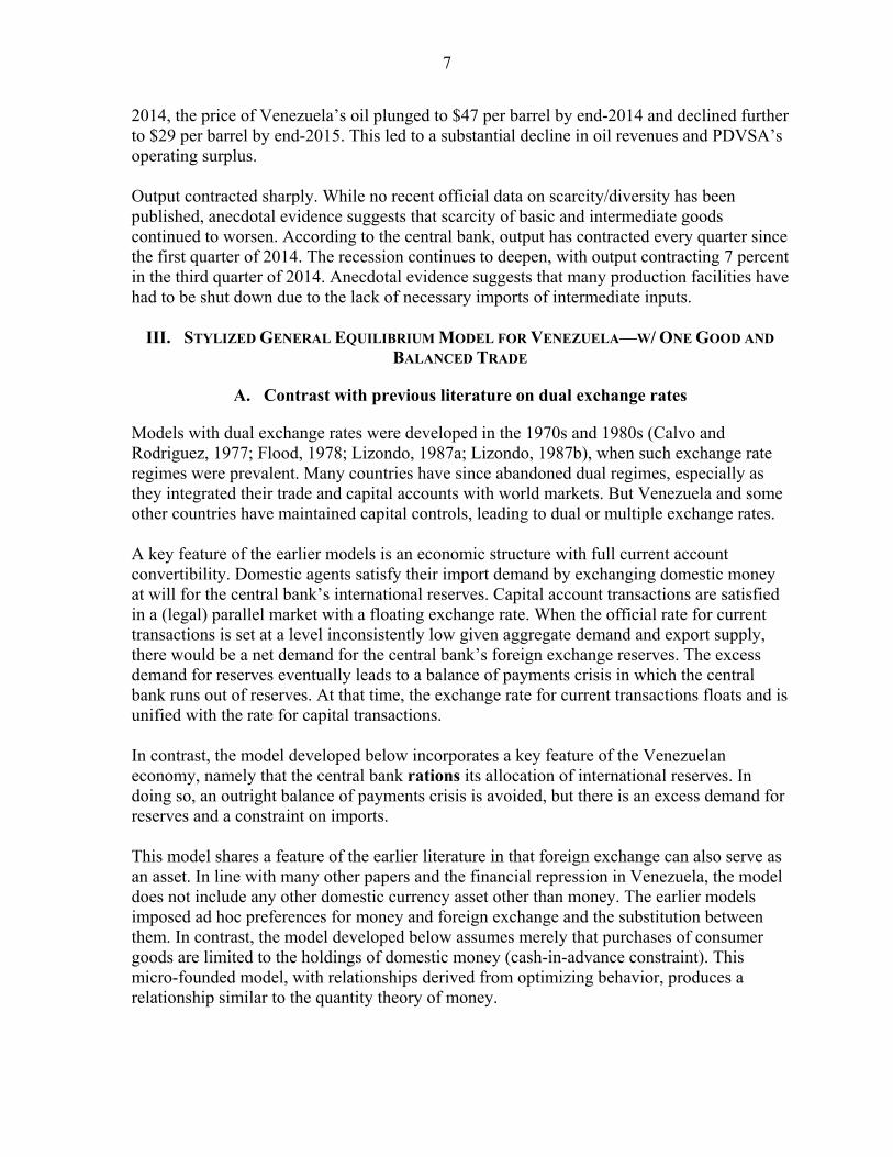
A. Contrast with previous literature on dual exchange rates

Models with dual exchange rates were developed in the 1970s and 1980s (Calvo and Rodriguez, 1977; Flood, 1978; Lizondo, 1987a; Lizondo, 1987b), when such exchange rate regimes were prevalent. Many countries have since abandoned dual regimes, especially as they integrated their trade and capital accounts with world markets. But Venezuela and some other countries have maintained capital controls, leading to dual or multiple exchange rates. A key feature of the earlier models is an economic structure with full current account convertibility. Domestic agents satisfy their import demand by exchanging domestic money at will for the central bank’s international reserves. Capital account transactions are satisfied in a (legal) parallel market with a floating exchange rate. When the official rate for current transactions is set at a level inconsistently low given aggregate demand and export supply, there would be a net demand for the central bank’s foreign exchange reserves. The excess demand for reserves eventually leads to a balance of payments crisis in which the central bank runs out of reserves. At that time, the exchange rate for current transactions floats and is unified with the rate for capital transactions. In contrast, the model developed below incorporates a key feature of the Venezuelan economy, namely that the central bank rations its allocation of international reserves. In doing so, an outright balance of payments crisis is avoided, but there is an excess demand for reserves and a constraint on imports. This model shares a feature of the earlier literature in that foreign exchange can also serve as an asset. In line with many other papers and the financial repression in Venezuela, the model does not include any other domestic currency asset other than money. The earlier models imposed ad hoc preferences for money and foreign exchange and the substitution between them. In contrast, the model developed below assumes merely that purchases of consumer goods are limited to the holdings of domestic money (cash-in-advance constraint). This micro-founded model, with relationships derived from optimizing behavior, produces a relationship similar to the quantity theory of money.

8

B. Summary of the basic structure of the economy

The structure of the model is designed to highlight the key features of the Venezuelan economy that lead to the rising inflation and black market premium. Other elements of the economy will be simplified if they are deemed not essential to the exposition. A public enterprise produces the only export good (oil), which is not consumed domestically. There are private sector firms that specialize in providing the imported consumption good (food), which is not produced domestically. Other private sector firms specialize in arbitraging foreign exchange between the official market and the black market. The government receives oil revenue from the public enterprise in dollars, and deposits these receipts in the central bank in exchange for domestic currency (bolivars) at the official exchange rate. The government makes lump-sum transfers to households in domestic currency. The central bank allocates its dollar receipts to the private sector at the official rate, through rationing. The fraction (1- φ) of the recipients of the central bank’s dollar allocations are import firms, but a fraction, φ, of the recipients are arbitrage firms, which in turn sell their dollars to importers in the black market. A holding company consolidates all profits and rents of the import firms and arbitrage firms, and fully distributes them to households each period. A detailed discussion of the model follows below.

C. External, fiscal, and monetary sectors

External sector Oil production and the dollar price of oil are exogenous, so the dollar value of export receipts, denoted Xt, is also exogenous each period. The stocks of foreign assets and external debt are initially zero, for both the public and private sector. The public sector fully distributes its export receipts to the private sector each period and does not issue external debt. In sections III-V, there is no accumulation of foreign assets, as the private sector uses the dollar allocations fully for payment of imports; therefore, trade is balanced each period. This assumption is relaxed in section VI to analyze the black market rate when some of the dollar allocation is used to build up portfolio holdings of dollars (capital flight) instead of being fully used for imports. The foreign price in dollars of the import good is constant at P*, and the quantity of the good imported is denoted Qt. In the case of no capital flows, balanced trade implies that the dollar value of the import good must equal the dollar value of export receipts. Therefore, the quantity of import goods is fixed at the amount determined from the exogenous export value and import price: (1) Qt = Xt / P*

9

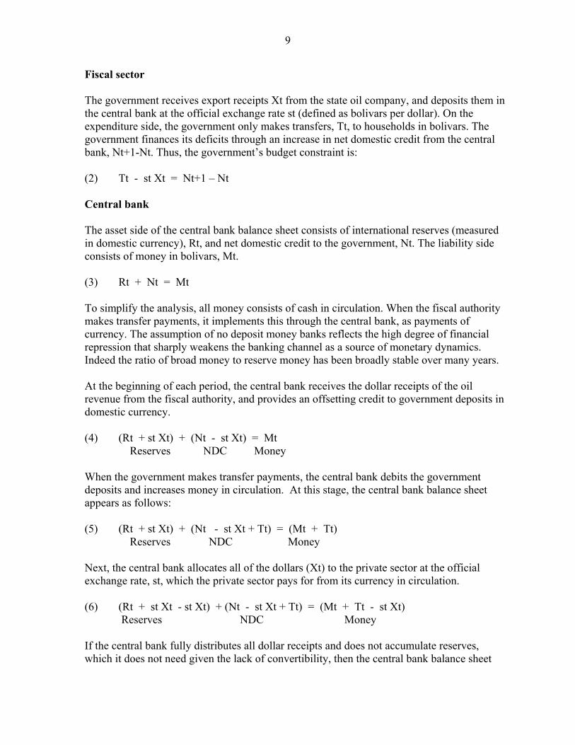
Fiscal sector The government receives export receipts Xt from the state oil company, and deposits them in the central bank at the official exchange rate st (defined as bolivars per dollar). On the expenditure side, the government only makes transfers, Tt, to households in bolivars. The government finances its deficits through an increase in net domestic credit from the central bank, Nt+1-Nt. Thus, the government’s budget constraint is: (2) Tt - st Xt = Nt+1 – Nt Central bank The asset side of the central bank balance sheet consists of international reserves (measured in domestic currency), Rt, and net domestic credit to the government, Nt. The liability side consists of money in bolivars, Mt. (3) Rt + Nt = Mt To simplify the analysis, all money consists of cash in circulation. When the fiscal authority makes transfer payments, it implements this through the central bank, as payments of currency. The assumption of no deposit money banks reflects the high degree of financial repression that sharply weakens the banking channel as a source of monetary dynamics. Indeed the ratio of broad money to reserve money has been broadly stable over many years. At the beginning of each period, the central bank receives the dollar receipts of the oil revenue from the fiscal authority, and provides an offsetting credit to government deposits in domestic currency. (4) (Rt + st Xt) + (Nt - st Xt) = Mt Reserves NDC Money When the government makes transfer payments, the central bank debits the government deposits and increases money in circulation. At this stage, the central bank balance sheet appears as follows: (5) (Rt + st Xt) + (Nt - st Xt + Tt) = (Mt + Tt) Reserves NDC Money Next, the central bank allocates all of the dollars (Xt) to the private sector at the official exchange rate, st, which the private sector pays for from its currency in circulation. (6) (Rt + st Xt - st Xt) + (Nt - st Xt + Tt) = (Mt + Tt - st Xt)

Reserves NDC Money If the central bank fully distributes all dollar receipts and does not accumulate reserves, which it does not need given the lack of convertibility, then the central bank balance sheet

10

carries no international reserves at the beginning and end of each period (Rt-1 = Rt = 0). Its balance sheet consists only of money and net domestic credit to the government. Thus at the end of the period, the central bank balance sheet appears as follows: (7) Rt = 0 (8) Mt+1 = Mt + Tt – st Xt (9) Nt+1 = Nt + Tt – st Xt By inspection, we see that money is created from the change in net domestic credit to the government, which is the fiscal deficit: (10) ∆Mt+1 = ∆Nt+1 = Tt – st Xt However, the equality between the increase in money and the fiscal deficit occurs only because the central bank sells all of its new reserves each period and because the private sector pays for dollars at the same official rate as is credited to the government for export receipts. Money creation will be higher if the central bank accumulates reserves. A higher volume of dollar sales to the private sector or a higher average exchange rate required for dollar purchases will reduce money growth. These relationships are illustrated with numerical examples in Appendix 2.

D. Firms

On the supply side, the market structure consists of a large number of import firms and arbitrage firms. Each firm is small and does not have power to set market prices of goods or the black market rate, but merely takes prices as given, as determined by the overall demand for goods in the retail market and dollars in the black market. For simplicity, I normalize the number of import and arbitrage firms to one representative firm in each market. Import firm The representative import firm buys (1- φ) Xt dollars from the central bank at the official rate st and buys φ Xt from the arbitrage firm at the black market rate bt. The dollars Xt can buy a maximum quantity Qt=Xt/P* of import goods at the international price P* and the firm, serving also as a retailer, sells the import goods in the domestic market at the bolivar price Pt. Therefore, the firm’s revenues are Pt Qt and its costs are the sum of payments to the central bank ((1- φ) st P* Qt) and to the arbitrage firm (φ bt P* Qt). (11) ∏ M t = Pt Qt - [ (1- φ) st + φ bt ] P* Qt Profits Rev Ave ex rt Cost at world price Although the representative import firm does not have power to set the market price (it is one small firm among many selling that particular good), rents persist because the central bank rations foreign exchange despite excess demand for it. In the model, the central bank does

11

not allocate dollars to the highest bidder, but makes its rationing decision based on arbitrary criteria. This implies that even though the market price for a good could be well above the marginal cost of supplying the good, firms cannot increase supply. Instead, supply is restricted by the need for foreign exchange, which is rationed. I also assume that the transformation of the import good into a retail good is costless. Therefore, the import firm will want to buy dollars from the central bank and use them to increase imports as long as the bolivar retail price equals or exceeds the domestic currency price of the import good at the official exchange rate: (12) Pt ≥ st P* Likewise, the import firm will want to buy dollars from the arbitrage firm as long as the bolivar retail price equals or exceeds the domestic currency price of the import good at the black market exchange rate: (13) Pt ≥ bt P* If the import firm had to incur a transformation cost per unit, ξt, (for transportation, distribution, retail service costs), then the domestic retail price would need to exceed the sum of the import cost and transformation cost: (12′) Pt ≥ st P* + ξt (13′) Pt ≥ bt P* + ξt For the remaining analysis, I assume ξt = 0. Arbitrage firm The representative arbitrage firm receives an allocation of dollars, φ Xt, from the central bank and sells it to importers in the black market, at the exchange rate bt. The arbitrage firm is willing to engage in this transaction as long as the black market rate it receives from the importer equals or exceeds the cost of dollars at the official exchange rate, where the rent is the difference between the black market receipt and the costs incurred. (14) ∏At = [ bt - st ] * φ Xt Profits MR - MC per dollar Amount transacted The import firm is willing to buy from the black market as long as the retail price equals or exceeds the black market rate (13). Competition among import firms for the dollars will drive this relationship to equality. Thus, in the case that black market dollars can be used only for imports and not for portfolio holdings (capital flight), the black market rate is bounded by the retail price and the official exchange rate: (15) Pt /P* = bt ≥ st

12

Holding company To ensure a complete flow of funds in general equilibrium, a holding company consolidates the profits (rents) of the import firm and the arbitrage firm and distributes these earnings to the representative household each period. (16) ∏t = ∏Mt + ∏At = Pt Qt - st P* Qt = [Pt – st P*] Qt

E. Households

The representative household has earnings from profits of the holding company and receives the transfer payment from the government. The household consumes the import good. The government successfully requires that retail sales of goods be purchased using domestic currency. Thus, the household is subject to a cash-in-advance constraint which requires money to pay for goods. The household maximizes a discounted stream of utility of consumption, subject to a budget constraint and the cash-in-advance constraint. (17) max∑ s.t. Mt+1 + Pt Ct = Mt + (Tt + ∏t) budget constraint and Mt ≥ Pt Ct cash-in-advance constraint Appendix 3 sets out the optimizing conditions. The discount rate, β, is slightly below unity (generally around 0.97-0.99) depending on the rate of time preference. Goods market clearing requires that Ct = Qt. Therefore, if the import volume is constant over time, the cash-in-advance constraint will be binding with any positive inflation rate. In this case, the price level is proportional to the money supply and inversely proportional to the quantity of imports. Summing the demand functions across households produces an aggregate demand curve: (18) Pt = Mt / Qt Aggregate demand curve Figure 1 illustrates the general equilibrium relationship, consisting of a fixed supply of import goods and the aggregate demand curve.

F. Equilibrium exchange rate

The concept of the equilibrium value of the official exchange rate is easy to determine in this framework. Given that the only consumption good is imported, the equilibrium nominal exchange rate is the value of st that satisfies the Law of One Price (LOOP), setting equation (12) to equality. (19) Equilibrium exchange rate: ̃t = Pt / P*

13

The equilibrium real exchange rate (= st P* / Pt) equals unity. Any value of st set lower than Pt/P* would imply an overvalued real exchange rate according to LOOP. When the official exchange rate is set at the equilibrium value under LOOP, the black market rate would be the same as the official rate. Combining equations (1), (18), and (19), assuming no capital flows, the equilibrium nominal exchange rate is related to money and export receipts. (20) ̃t = Pt / P* = [ Mt/ (Xt/P*) ] / P* = Mt / Xt An increase in the money supply has a proportionate increase (depreciation) in the equilibrium nominal exchange rate. Figure 2 illustrates this case. An increase in export receipts, which provides for a greater supply of import goods, leads to a decline (appreciation) in the equilibrium nominal exchange rate. If the official exchange rate is overvalued, such that (12) does not hold with equality, the import firm will earn rent. A devaluation of the official exchange rate to another level below or equal to the LOOP level would entail a reduction in the rent that the import firm receives. As long as the new level of the official rate is still at or below the LOOP equilibrium level, the retail price Pt won’t rise (see Figure 3). The lack of pass-through from the devaluation arises because the retail price (set at the level corresponding to the demand for the import good in the context of a fixed supply of the import good) is above the cost of supplying the good. However, the devaluation will result in lower rents received by the import and arbitrage firms, leading to lower household income and a subsequent reduction in prices. A very large devaluation of the official exchange rate could lead to an increase in the price level if it significantly raises the import cost of the good such that an increase in the retail price of the good is required to ensure LOOP (Figure 4). Otherwise, if importers started making losses, they would cut back on supply, which would increase prices. In summary, the demand side of the economy is driven by money growth, which in turn depends mainly on fiscal deficits, as well as the central bank policies for reserve accumulation and allocation of foreign exchange to the private sector. The supply side of the economy is driven by the receipt of dollars from export earnings, which are distributed to importers and arbitrageurs through the central bank.

IV. CALIBRATIONS AND DYNAMIC SIMULATIONS OF ONE GOOD MODEL

A. Calibration of black market exchange rate

Equation 20 provides a simple relationship for the equilibrium exchange rate, given the law of one price and the structure of the Venezuelan economy. The model predicts that the equilibrium exchange rate will equal the domestic money supply divided by the foreign exchange allocated for imports. In the one good model, equation (15) shows that a similar relationship would hold for the black market rate.

14

I calibrate the model to Venezuelan data available for mid-2015, based on the following information and sources: Venezuela’s broad money has risen from 715 billion bolivars at end 2012 to a

projected 2,335 billion bolivars (assuming 65 percent growth in broad money y/y). GlobalSource Partners estimates that total FX sales peaked in 2012 at $170m per day,

falling to $130m per day in 2013, $90m per day in 2014, and $30 million per day in May 2015. These figures imply annual FX allocations of $62 billion in 2012, $48 billion in 2013, $33 billion in 2014, and $11 billion (annualized) in May 2015.

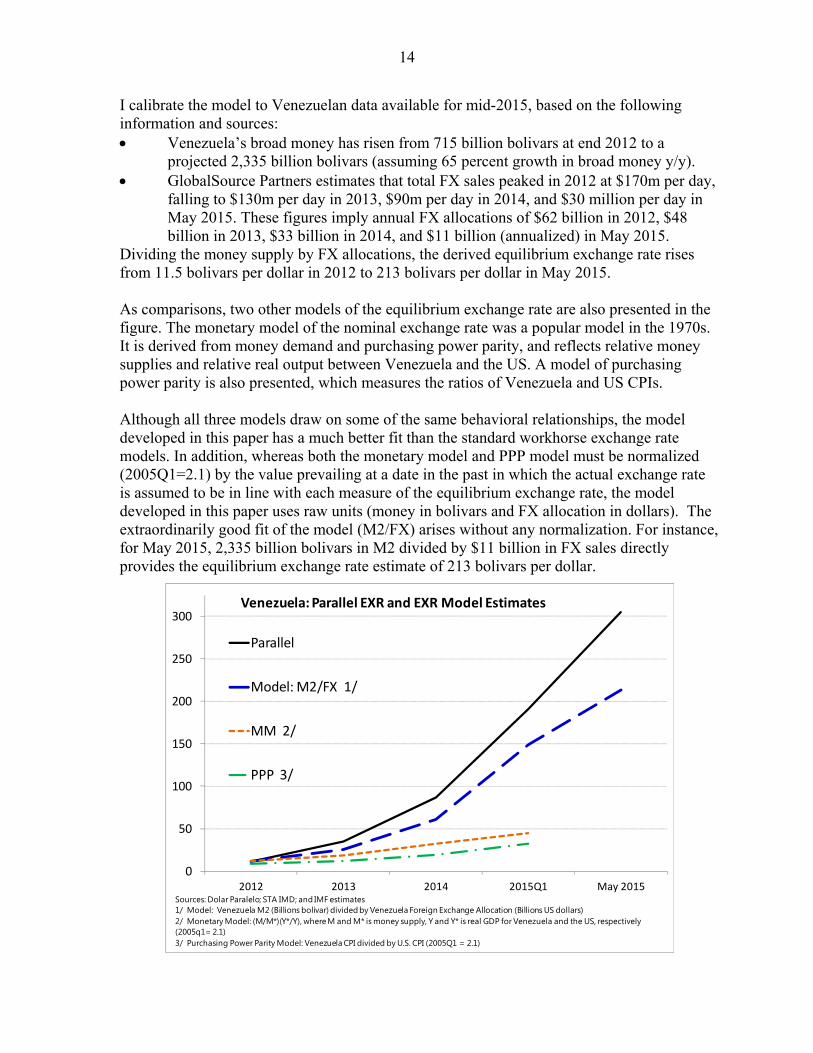
Dividing the money supply by FX allocations, the derived equilibrium exchange rate rises from 11.5 bolivars per dollar in 2012 to 213 bolivars per dollar in May 2015. As comparisons, two other models of the equilibrium exchange rate are also presented in the figure. The monetary model of the nominal exchange rate was a popular model in the 1970s. It is derived from money demand and purchasing power parity, and reflects relative money supplies and relative real output between Venezuela and the US. A model of purchasing power parity is also presented, which measures the ratios of Venezuela and US CPIs. Although all three models draw on some of the same behavioral relationships, the model developed in this paper has a much better fit than the standard workhorse exchange rate models. In addition, whereas both the monetary model and PPP model must be normalized (2005Q1=2.1) by the value prevailing at a date in the past in which the actual exchange rate is assumed to be in line with each measure of the equilibrium exchange rate, the model developed in this paper uses raw units (money in bolivars and FX allocation in dollars). The extraordinarily good fit of the model (M2/FX) arises without any normalization. For instance, for May 2015, 2,335 billion bolivars in M2 divided by $11 billion in FX sales directly provides the equilibrium exchange rate estimate of 213 bolivars per dollar.

0

50

100

150

200

250

300

2012 2013 2014 2015Q1 May 2015

Venezuela: Parallel EXR and EXR Model Estimates

Parallel

Model: M2/FX 1/

MM 2/

PPP 3/

Sources: Dolar Paralelo; STA IMD; and IMF estimates1/ Model: Venezuela M2 (Billions bolivar) divided by Venezuela Foreign Exchange Allocation (Billions US dollars)2/ Monetary Model: (M/M*)(Y*/Y), where M and M* is money supply, Y and Y* is real GDP for Venezuela and the US, respectively(2005q1= 2.1)3/ Purchasing Power Parity Model: Venezuela CPI divided by U.S. CPI (2005Q1 = 2.1)

15

B. Dynamic simulations of inflation

The model can also be used to conduct policy experiments to simulate inflation dynamics under alternative fiscal and exchange rate policies. Fiscal policy consists of the growth rate of transfer payments (t), whereas exchange rate policy consists of the devaluation rate (s).The summary of the model equations and initial values for the simulation are presented in Appendix 4. Impact of fiscal policy The first scenario assumes that the growth rate of spending and the annual devaluation rate

are both constant at 25 percent = 25%). In this case, money growth and inflation

reach a steady state when /

. If the initial deficit to money ratio is

higher than the steady state ratio, inflation will be above its steady state. It will fall over time and converge to its steady state rate of 25 percent. If the rate of spending growth and devaluation rises to 95 percent, the initial deficit to money ratio will be lower than its steady state ratio. Inflation will also be below its steady state and will rise over time until it converges to its steady state of 95 percent.3

Impact of one-off devaluation of official exchange rate In this scenario, the growth rate of spending (Tt) is 25 percent, but the official exchange rate is held at 6.3 bolivars per dollars for four years. In year 5, the official exchange rate is devalued from 6.3 to 15, without changing the nominal growth of spending. The devaluation reduces the fiscal deficit by increasing the bolivar value of oil revenues. As a result, the government’s need for monetary financing falls. With a lower amount of money supply, aggregate demand and inflation fall relative to the counterfactual case of no devaluation.

3 This scenario is an example of fiscal dominance, in which the fiscal deficits drive money creation and inflation (see Sargent and Wallace, 1981).

Impact of Fiscal Policy

0

5

10

15

20

25

30

35

1 5 9 13 17 21 25 29 33 37

==25%

inflation

deficit (% M)

0

10

20

30

40

50

60

70

80

90

100

1 5 9 13 17 21 25 29 33 37

==95%

inflation

deficit (% M)

16

Thus, the short-run effect of the devaluation is much lower inflation. However, since spending growth remains at 25 percent, inflation still converges to the long-run steady state level of 25 percent. The temporary rebound in inflation in the transition to the steady state is explained by the fact that the real value of government spending increases when inflation falls relative to the no-devaluation scenario.

Why doesn’t the devaluation pass through to higher prices? The reason is that the market structure is not characterized by perfect competition or monopolistic competition. The market structure is something different—a repressed goods market. Foreign exchange is required to purchase imports and it is allocated through official discretion, not through a market mechanism. Firms fortunate enough to obtain foreign exchange at the official rate are able to extract rents that cannot be competed away. So, they can keep the price of a good well above its cost to import. New firms cannot enter to drive away rents. When the official rate is

One-off Devaluation

0

1000

2000

3000

4000

5000

6000

7000

1 3 5 7 9 11 13 15 17 19 21 23 25 27 29

bt/st - no deval

bt/st - deval

0

1

2

3

4

5

6

7

8

9

1 3 5 7 9 11 13 15 17 19 21 23 25 27 29

Tt/Pt - no deval

Tt/Pt - deval

15

20

25

30

35

40

1 3 5 7 9 11 13 15 17 19 21 23 25 27 29

Inflation- no deval

Inflation - deval

Deficit/Mt - no deval

Deficit/Mt - deval

17

devalued, it only reduces rents. It does not necessarily raise prices. In fact, the reduction in rents (subsidies) takes away purchasing power from some domestic agents, reducing aggregate demand. The existence of a black market for foreign exchange does not change this phenomenon. The black market shifts wealth around within the country, but does not change the basic foreign exchange constraint imposed by the government that maintains rents and an excess demand for foreign exchange. Impact of devaluation cycles In the past, Venezuela’s official exchange rate has repeatedly been devalued after being held fixed for a period of more than a year. This scenario shows how the deficit (relative to the money supply) and inflation evolve when the exchange rate is devalued every five years. In the first case, fiscal spending grows each year by 25 percent. Every five years, the official exchange rate is devalued by the cumulative growth in spending over five years (205 percent). Each time the exchange rate is devalued, the fiscal deficit and inflation fall temporarily. But since spending continues to growth by 25 percent, the deficit and inflation soon rise again. Inflation cycles around the long-run average of 25 percent. If fiscal spending growth is higher—such as 95 percent—inflation will cycle around the higher level. As above, the deficit and inflation fall in the year of the devaluation and rise again afterward.

Impact of a real shock: oil revenue decline The model can also simulate the impact of the sharp decline in oil prices, which has represented a critical real shock to Venezuela. Given the collapse in oil prices, foreign exchange has plummeted, leaving few resources for imports. In fact, as illustrated in Figure 5, the fall in oil revenue combines two effects that increase inflation. Lower oil revenue implies that the government has a higher deficit and must use more monetary financing. In addition to the increase in money, the fall in oil prices requires lower imports and thus a lower supply of goods to the domestic market.

Devaluation Cycles

0

5

10

15

20

25

30

35

40

45

1 5 9 13 17 21 25 29 33 37

=25

inflation

deficit (% M)

0

20

40

60

80

100

120

1 5 9 13 17 21 25 29 33 37

=95

inflation

deficit (% M)

18

This scenario is calibrated to be similar to recent developments in Venezuela. Values of the money stock, export receipts, the fiscal deficit and inflation are broadly in line with developments from 2014. Going forward, fiscal spending growth is assumed to grow at 95 percent, roughly the observed rate of money growth in 2015. In addition, oil prices are assumed to drop from an average of about $88 per barrel in 2014 to $50 per barrel in 2015 and $30 per barrel in 2016. Based on these assumptions, the simulation of the model shows that inflation would shoot up to over 200 percent in 2015 and 2016 before beginning to converge back to the steady state level of 95 percent, driven by fiscal spending growth.

V. BLACK MARKET WITH MULTIPLE CONSUMPTION GOODS

A. The consequence of multiple goods

The one good model has provided a useful framework to understand inflation dynamics in Venezuela. It demonstrates the impact of fiscal spending, oil receipts, and devaluation of the official exchange rate. The model also goes a long way in explaining the rise in the black market rate. However, the rise in the black market rate has been much higher than overall inflation, and the gap with the fitted value of the equilibrium exchange rate has been widening. In order to fully understand the steep increase in the black market exchange rate in Venezuela in the last few years, it is necessary to consider a model with more than one consumption good. In addition, the black market rate will depend on the amount of foreign exchange transactions taking place in the market relative to the amount of imports. Thus, this section extends the model to multiple goods, with only a small share of transactions taking place in the black market. Imagine a large number of importing firms competing to buy a portion of the dollars available in the black market. They intend to purchase goods i=1…N from the international markets and sell the goods in the domestic retail market. Each firm is small enough to be a price taker in the domestic market, but all of the firms combined will affect the price of the good. Each firm will consider the profits it could receive by selling good i: (21)

∗

Profits of an individual firm will therefore increase as long as ∗

0

50

100

150

200

250

2013 2015 2017 2019 2021 2023

Export Revenue Shock

inflation - no X fall

inflation - X fall

19

An arbitrageur will choose to sell its dollar receipts to the highest bidders among import firms. For any good i, the break even black market rate will set price equal to cost.

(22) ∗

or ∗

Arranging goods in the order 1…n based on the markups,

(23) ∗ ∗ ∗ ⋯ ∗ Importers of good 1 will be willing to buy dollars at the black market rate until P1 is driven

down to ∗ ∗ and so on. If goods importers are segmented, the black market rate will

reflect the markets with the highest markups over the international price. A reduction in transactions in the black market will raise the black market rate because only the most distorted (highest markups) markets will receive dollar funding. If a monopolist firm makes all the import decisions, it will use the foreign exchange to import each good until the ratio of marginal revenue to marginal cost is equal across goods.

B. Two goods model

Based on the discussion above, the model is revised to the case of multiple imported consumption goods, where two goods is sufficient to illustrate the points. As before, there are firms that import goods and firms that arbitrage dollars in the black market. The central bank allocates (in an ad hoc manner) foreign exchange at the official exchange rate, st, to import firms that purchase the two import goods from foreign markets at a fixed world price. As long as the domestic price (Pit), which constitutes marginal revenue, is above the domestic value of the foreign price (st Pit*), which constitutes marginal cost, the importing firm will want to supply the good. The central bank also allocates a share, , of dollar export receipts to arbitrage firms at the official exchange rate, st. The arbitrageurs sell the dollars in the black market at the highest possible exchange rate. The household’s intertemporal optimization problem now includes utility of two consumption goods. (24) max∑ ,∞ s.t. ∏ budget constraint and cash-in-advance constraint Appendix 5 elaborates the solution. For example, if the CIA constraint is binding and utility is logarithmic, then the expenditure shares on each good are equal.

20

(25) Also, the black market rate grows proportionately to spending on each good.

(26)

C. Simulation of black market rate in two goods model

The central bank supplies dollars through rationing in proportion to the export revenues (Xt) deposited by the government from earnings of the state oil company. As before, the central bank allocates a fraction, 1-φ, to importers and a fraction, φ, to arbitrageurs. Since the capital account is restricted, the only capital transactions that occur take place in the black market. Arbitrageurs supply dollars to the black market, which are used for imports of the two goods. Goods markets clear, such that imports, Qit, equal consumption of imported goods, Cit. The black market rate will mirror price increases in the most distorted good market, i.e., the one with the highest markup (Figure 6). This market is not necessarily the one with the highest inflation always, but rather with the highest margin between cost and price. The arbitrage firms will earn the greatest rent by selling their dollars to import firms that supply goods in the most distorted market. Table 1 provides a baseline calibration of the model. Fiscal transfers are assumed to grow by 50 percent, which drives money growth and spending of roughly the same magnitude. In 2015 and 2016, export revenues drop sharply, causing a contraction in foreign exchange allocated for imports. Foreign exchange provision is assumed to drop more sharply for good 2, driving up its price by more than three times that of good 1. The black market rate reflects the large markup in good 2 and rises with its higher inflation rate. Thus, the growth of the black market exchange rate is much above overall inflation. Arbitrage and import firms both earn rents from selling dollars and goods, respectively. If the share of dollars channeled through the black market increases, it could lead to a decline in the black market rate because it will increase the supply of goods in the distorted market and thus reduce their price. The distorted market will become slightly less distorted. If arbitrageurs buy dollars from importers in the less distorted market and sell them to importers in the more distorted market, it would lead to a change in the composition of goods. Supply in the more distorted market would increase and the price would decline, while the opposite would hold in the other market. Instead of the idea that prices of goods reflect the black market rate (firms pricing at the black market rate), we should think of the converse: the black market rate is based on retail goods prices. But the black market exchange rate can grow faster than overall inflation if price increases for goods in the most distorted markets is higher than goods in less distorted markets.

21

Figure 8 shows the simulation from an increase in the amount allocated to the black market (in 2016). Dollars are used to substitute additional imports of good 2 (the relatively scarce good) by reducing imports of good 1 (the relatively abundant good). The contemporaneous rate of inflation in good 2 is reduced, while inflation rises somewhat for good 1. Overall inflation is lower than the baseline and the black market rate grows significantly less. Welfare improves since the rise in the utility of consumption of the scarce good is greater than the fall in the utility of consumption of the less scarce good.

D. Simulation of a devaluation

Figure 9 shows the impact of a devaluation of the official exchange rate from 6.3 to 50 (in 2017). The deficit significantly reduces the fiscal deficit, facilitating a decline in money growth. In addition, arbitrageurs and importers incur higher costs of purchasing foreign currency, which reduces their profits. The lower profits transferred as income to households leads them to reduce their subsequent spending on both goods, which leads to lower inflation and lower black market exchange rate than in the baseline.

VI. CAPITAL FLIGHT

Until this point, the model assumed balanced trade, or equivalently, no capital flows or changes in net foreign assets. However, even if the government prevents domestic firms and individuals from establishing financial accounts overseas, it may not be able to prevent capital flight in the form of accumulation of dollar holdings. Import firms may engage in overinvoicing to save some of the foreign exchange allocation. Arbitrageurs can also speculate by choosing to hold the dollars until a later period. The model can be extended to accommodate capital flight. Appendices 6 and 7 present the technical details. Changes in the stock of dollars held by domestic households must equal the difference between the total amount of dollars the central bank distributes from export revenues and the value of imports. (27) Ft+1 - Ft = Xt – P1* Q1t-P2*Q2t This extended model can also be simulated to show the impact of capital flight on inflation, the black market rate, and welfare.

A. Simulation of overinvoicing and dollar savings by importers

An importing firm that sells both goods (or can sell dollars to an importer in the other goods market) has the incentive to overinvoice imports so as to acquire dollars from the central bank at the official exchange rate, and then use the dollars to import goods in the distorted market now or in the future. If FX is expected to become scarcer in the distorted market next period, import firms could try to reduce their imports in the less distorted market this period and use the dollars to increase imports in the distorted market next period. Figure 10 illustrates this scenario and shows that the temporary capital flight that is used to raise supply in the subsequent period of increased scarcity improves overall welfare. In general equilibrium, the revenue the importers would earn would be the same after the change in quantity supplied because the price would change in inverse proportion. However,

22

the cost of acquiring dollars from arbitrageurs would fall because the black market rate and the price of the good in the distorted market would decline when its supply increases.

B. Simulation of black market dollar savings (capital flight) by arbitrageurs

Figure 11 shows the results of a simulation of capital flight by arbitrageurs. If the black market rate is expected to increase (by enough to offset any time discount factor), arbitrageurs could save a dollar in the current period t—losing bt revenue per dollar—and then sell that dollar in the next period t+1—gaining bt+1 revenue per dollar. They would gain extra profits at the expense of the importing firm. They would have the incentive to do this up until the point in which the black market rate is equalized between t and t+1. This increase in dollar savings constitutes capital flight during the period of saving. It also implies that current high increases in the black market rate could reflect not only lower imports due to a fall in export receipts but also the voluntary withdrawal of dollars for import now because of an expectation that they will become even more restricted in the future. Since dollars are saved this period by reducing imports to the distorted market, this would increase the price of the good this period and reduce it next period. This exchange of imports through time would smooth out imports (and consumption) from the current high level to the future lower level. This would improve welfare.

VII. EXTENSIONS OF MODEL

A. Price controls

Suppose that there are two consumption goods, but the price of one good is constrained by a price control. Assuming that the cash-in-advance constraint holds, as argued above, we can simplify the household’s decision on the allocation of consumption between the two goods to a static allocation problem each period. (28) max ,

s.t. M = P1 C1 + P2 C2 cash-in-advance constraint

and price control In the case when the price control is not binding, the FOC would give: (29) U1 / U2 = P1 / P2 For example, if U(C) = log ( ) + log ( ), then the household would like to spend equal shares of the money budget on each good. (30) P C P C However, aggregate consumption of each good is constrained by its import supply, which in turn depends on the rationed foreign exchange allocation received by the importers of the goods. If firms are free to set retail prices, the relative prices will be determined by the

23

relative supply of goods and optimality condition (29). The overall price level will be determined by aggregate household spending, which is given by the money supply. However, if the price control is binding such that the price of good 2, , is forced below the optimal retail price, then there will be excess demand for good 2 that will produce a shortage (Figure 7). In addition, with restricted supply and controlled price of good 2, households will have unsatisfied spending power that will spill over into additional demand for good 1 and increase its price beyond the level that would prevail in the absence of the price control on good 2. In particular, the price of the non-controlled good, P1, will be determined by the money supply and import supplies of the two goods. (31) P M Q /Q An increase in the controlled price of good 2 (i.e., a relaxation of the binding constraint) or an increase in its import volume would reduce the equilibrium retail price of good 1. In this case, the optimality condition (29) may not hold.

B. Nontraded good

The model can also be extended by adding a non-traded good produced with inelastic labor. (32) A representative firm maximizes profits The wage rate is thus tied to the price of the non-traded good: The household optimization now includes utility of both consumption goods. (33) max∑ ,∞

s.t. ∏ budget constraint

and cash-in-advance constraint As shown in Appendix 8, the rate of inflation must be at least as high as the discounted marginal rate of substitution in consumption.

(34) ,

,

In addition, there is another first order condition relating the marginal utility of each consumption good.

(35) ,

,

If utility is logarithmic, then the expenditure shares on each good are equal.

24

(36) Further assume that the inelastic labor supply = 1. Then, 1 and

(37)

The relative price of the non-traded good increases when consumption of the traded good increases. In other words, the relative price of the non-traded good must rise in order to induce households to optimally choose a fixed consumption of the non-traded good when consumption of the traded good rises. This result is in line with the usual intuition on the real exchange rate. When national wealth increases—due to higher export receipts in Venezuela’s case—the real exchange rate (relative price of non-traded to traded goods) rises. The higher export receipts allow more imports of traded consumption goods. Conversely, when export wealth falls, the equilibrium real exchange rate also falls.

C. Imported intermediate input

Instead of assuming that the retail consumer good is a direct import good, the model can be extended by requiring that the import is an intermediate input that must be combined with domestic labor in order to assemble the retail consumer good. So there is a production function for output. (38) where is the firm’s use of the imported intermediate good. The representative firm is assumed to be a price taker and maximizes its profits, choosing the optimal quantity of labor and the imported intermediate. (39) , ∗ The firm will choose labor such that the marginal produce of labor equals the wage,

(40) 1

and the imported intermediate such that the domestic currency cost of the input equals its marginal product.

(41) ∗

If total labor supply is inelastic, L=1, then aggregating across firms gives (42) 1

(43) ∗

25

The zero-profit black market exchange rate also changes slightly. Instead of reflecting only the ratio of the domestic price to the foreign price of the good, the black market rate also now depends on the overall quantity of the import good. The increase in the black market rate reflects domestic and foreign inflation and the growth of imports.

(44) ∗

∗

A fall in Q leads to a higher growth in the black market rate compared with inflation. The aggregate demand curve can now be expressed in terms of output (45) If the intermediate input is reduced because of lack of foreign exchange allocation, it also lowers the output of the retail good. There is a direct link between output, consumption, and the import good. However, consumption and output growth are less volatile than the import good. In fact, this relationship is clearly evident in Venezuela over the past, with output, private consumption, and import growth moving closely together. However, as predicted by this model, import growth rates would be larger in absolute value than output and consumption growth rates.

D. Other macro policies

Government spending in dollars If the government purchases foreign goods and services using dollars, it will decrease the supply of dollars for import of the consumption good. Thus, Qt will fall. The effects will be

-45

-30

-15

0

15

30

45

60

-15

-10

-5

0

5

10

15

20

19

98

19

99

20

00

20

01

20

02

20

03

20

04

20

05

20

06

20

07

20

08

20

09

20

10

20

11

20

12

20

13

20

14

Venezuela: Real Growth Rates

Private Consumption

GDP

Imports (rhs)

26

similar to a reduction in Xt, unless government purchases are used to satisfy consumption demand. Issuance of external debt If the government issues external debt, it increases the availability of foreign exchange for import, thus raising Qt in the short run. However, it will have to pay back the debt, thus reducing Q in the future. Likewise, payment of external debt service reduces the availability of foreign exchange for import, further driving up inflation and the black market rate. Issuance of domestic debt If the government finances its deficit by issuing domestic debt, it reduces the amount of monetary financing required. Thus, the money supply will be lower by the amount of debt sold compared with the counterfactual of no debt issuance. However, the government will have to pay back the debt in the future, so future money supplies will be increased again. Accumulation of foreign exchange reserves If the central bank builds foreign exchange reserves instead of selling them, then the money supply will be higher than it would be compared with the sale of reserves. In addition, there will be less foreign exchange available for imports. Likewise, a reduction in foreign exchange reserves through sale to domestic agents would reduce the money supply and increase imports. Thus, a scenario with an accumulation of foreign exchange reserves would show higher inflation and lower consumption relative to a scenario when foreign exchange reserves are fully sold to domestic agents. Conversely, decumulation of reserves would produce more imports and lower inflation.

VIII. CONCLUSIONS

This paper presents a stylized general equilibrium model that captures the key features of the Venezuelan economy. The rationing of foreign exchange for imports, linked to oil export earnings, and a multiple exchange rate regime lead to a repressed market for consumer (and intermediate) goods. In this setting, the demand for consumer goods and foreign exchange availability determine the domestic price of the consumer good. The price of the consumer good then determines the black market exchange rate. In the more realistic situation of multiple goods, the arbitrary allocation to import and arbitrage firms creates varying levels of subsidies, and the black market rate will reflect the subset of goods with the highest markup over international prices. Capital flight (or equivalently, a portfolio choice between dollars and domestic currency) can also contribute to the dynamics, but is not needed to explain the rise in inflation and the even steeper surge in the black market premium. The model also explains two counterintuitive phenomen: (1) a fall in oil revenues can lead to a temporary increase in inflation, and (2) a devaluation can generate a temporary drop in inflation.

27

REFERENCES

Cagan, Phillip, 1956, “The Monetary Dynamics of Hyperinflation,” in Milton Friedman (ed.), Studies in the Quantity Theory of Money University of Chicago Press.

Calvo, Guillermo A., and Carlos Alfredo Rodriguez, 1977, “A Model of Exchange Rate

Determination under Currency Substitution and Rational Expectations,” Journal of Political Economy 85 (3), pp. 617-625.

Clower, Robert W., 1967, “A Reconsideration of the Microfoundations of Monetary

Theory,” Western Economic Journal 6, pp. 1-8. Flood, Robert R., 1978, “Dual Exchange Markets,” Journal of International Economics 8,

pp. 65-77. Guerra, Jose and Julio Pineda, 2000, “Trayectoria de la Política Cambiaria”. Vicepresidencia

de Estudios. Banco Central de Venezuela. Guerra, Jose and Julio Pineda, 2004, Temas de Política Cambiaria en Venezuela. Colección

Economía y Finanzas. Banco Central de Venezuela. Hausmann, Ricardo, 1990, Shocks Externos y Ajuste Macroeconómico. Colección

Cincuentenario. Banco Central de Venezuela. Lizondo, Jose Saul, 1987a, “Unification of Dual Exchange Markets,” Journal of

International Economics 22, pp. 57-77. _____, 1987b, “Exchange Rate Differential and Balance of Payments under Dual Exchange

Markets,” Journal of Development Economics 26, pp. 37-53. Sargent, Thomas, and Neil Wallace, 1981, “Some Unpleasant Monetarist Arithmetic,”

Federal Reserve Bank of Minneapolis Quarterly Review 5 (3), pp. 1-17.

28

APPENDICES Appendix 1. The Cagan Model—Not the Best Explanation for Inflation Surge

According to the Cagan model, hyperinflation is driven by severe drops in money demand dominated by rising inflation expectations. This phenomenon could be due to a rise in money growth that feeds inflation expectations and/or an increased elasticity of real money demand to expected inflation. The combination destabilizes inflation expectations and velocity rises. The Cagan model does not yet appear to fit Venezuela data. At least through 2014, there is no evidence that velocity was increasing or that the elasticity of money demand rose. In fact, velocity has been on a steady decline, irrespective of whether it is measured using GDP, aggregate demand, private consumption, or imports. The data for 2015 is incomplete. At end-December, the monetary base grew by 111 percent yoy and consumer price inflation reached at least 180 percent by the end of the year. On the surface, the increase in inflation above money growth may show the first signs that velocity has finally started to rise and the Cagan model is relevant. However, national accounts data, including GDP and its components, has not been published yet for 2015, so velocity cannot be updated at this time. The assumptions of the Cagan model may not fit Venezuela’s economic situation. First, the Cagan model assumes that real GDP is constant and simplifies to a relationship between money and expected inflation. This is an unrealistic assumption for Venezuela in 2015, as real GDP is estimated to have fallen sharply (based on indicators of activity). Real private consumption and imports may have fallen even more than output. Since the Cagan model does not account for this important development, the estimates from the model are not reliable. Second, the Cagan model is based on a money demand equation involving the choice between money and bonds.

where i is the nominal interest rate and The model assumes that Y and r are fixed and derives a relationship between M, P, and . The Cagan model may not fit Venezuela’s economic structure because of financial repression. It is likely that households do not have the option of buying bonds as an alternative asset to holding money.

-

5

10

15

20

25 2

00

0

20

01

20

02

20

03

20

04

20

05

20

06

20

07

20

08

20

09

20

10

20

11

20

12

20

13

20

14

Velocity = X / MoneyGDP

Domestic demand

Private consumption

Imports

29

Appendix 2. Numerical example of monetization of deficits, devaluation, and sales of reserves by the central bank.4

All scenarios assume that the government earns export revenue equal to 100 dollars and spends 2000 bolivars on transfer payments to households. The official exchange rate is 6 bolivars per dollar, and in some scenarios is devalued to 8 bolivars per dollar. I. Initial NIR = 0 No devaluation. Central bank builds reserves.

Beginning End Assets Liabilities Assets Liabilities

0 NIR 0 MB +600 NIR +2000 MB

0 DC gov 0 Dep gov 0 DC govt +600 -1400 Dep gov -2000

Devaluation. Central bank builds reserves.

Beginning End Assets Liabilities Assets Liabilities

0 NIR 0 MB +800 NIR +2000 MB

0 DC gov 0 Dep gov 0 DC govt +800 -1200 Dep gov -2000

Punchline: If the central bank does not sell dollars, money creation is determined only by government transfers. II. Initial NIR = 100 dollars No devaluation. Central bank sells dollars.

Beginning End Assets Liabilities Assets Liabilities

+600 NIR +2000 MB 0 NIR +2000 1400 MB -600

0 DC gov -1400 Dep gov 0 DC govt -1400 Dep gov 4 This illustration decomposes net domestic credit into domestic credit and government deposits, with the latter shown as a liability. “OIN” is other items net.

30

Devaluation. Central bank sells dollars. Beginning End

Assets Liabilities Assets Liabilities +800 NIR +2000 MB 0 NIR +2000 1200 MB

-800

0 DC gov -1200 Dep gov 0 DC govt -1200 Dep gov No devaluation for govt, but central bank sells dollars to private sector at devalued rate.

Beginning End Assets Liabilities Assets Liabilities

+600 NIR +2000 MB 0 NIR +2000 1200 MB -800

0 DC gov -1400 Dep gov 0 DC govt -1400 Dep gov

0 OIN -200 OIN

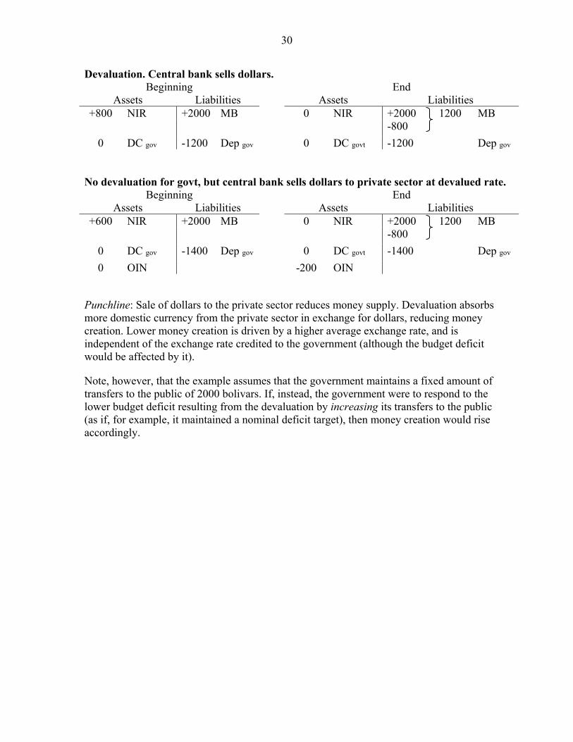
Punchline: Sale of dollars to the private sector reduces money supply. Devaluation absorbs more domestic currency from the private sector in exchange for dollars, reducing money creation. Lower money creation is driven by a higher average exchange rate, and is independent of the exchange rate credited to the government (although the budget deficit would be affected by it).

Note, however, that the example assumes that the government maintains a fixed amount of transfers to the public of 2000 bolivars. If, instead, the government were to respond to the lower budget deficit resulting from the devaluation by increasing its transfers to the public (as if, for example, it maintained a nominal deficit target), then money creation would rise accordingly.

31

Appendix 3. Household optimization with one good and CIA constraint

The household maximizes discounted utility of consumption, subject to a budget constraint and a constraint that purchases in a period are limited by money holdings. max∑

s.t. Mt+1 + Pt Ct = Mt + (Tt + ∏t) budget constraint and Mt ≥ Pt Ct cash-in-advance constraint (CIA)

Letting λt be the Lagrange multiplier associated with the cash-in-advance constraint, the Kuhn Tucker conditions require that:

0

Rearranging:

0

Since λt ≥ 0, it follows that the rate of inflation must be at least as high as the discounted marginal rate of substitution in consumption.

Solving the model with a CIA constraint implies that private consumption spending is either equal to or less than the money stock. Mt ≥ Pt Ct (Case 1) When the CIA constraint binds, consumption spending equals the money stock Mt = Pt Ct Inflation is proportional to the growth of money and inversely proportional to the growth of consumption.

MM

If money grows at rate , then inflation also grows at rate adjusted for the inverse of consumption growth.

1 μ

32

(Case 2) If the CIA constraint does not bind, consumption spending is less than the money stock, Mt > Pt Ct. In this case, inflation must equal the marginal rate of substitution between consumption this period and last period adjusted for the time preference.

Under isoelastic utility, , and

β

Under log utility (=1), this would reduce to

β

Inflation would be inversely related to consumption growth. When Case 2 holds and consumption (Ct=Qt) is either constant or increasing, inflation would be negative since beta is less than one (<1). Consumption could be constant or increasing if foreign exchange constraints and foreign borrowing constraints exist. In that situation, an increase in oil revenue could relax the import restriction, allowing an increase in consumption. Note that an increasing path of consumption is not an optimal policy if foreign constraints are not present. When the CIA constraint does bind,

β

or β

Appendix 4. Summary of model equations for dynamic simulations

The following equations summarize the dynamic equilibrium for the Venezuela model:

(A.1) Mt = Pt Ct when ′

′ Aggregate demand

or

(A.1′) Mt > Pt Ct when ′

′

(A.2) Ct = Qt Goods market clearing (A.3) ∆Mt+1 = Tt – st Xt Money growth tied to fiscal deficit

(assumes no change in reserves)

33

(A.4) Xt = P*t Qt Balanced trade (A.5) bt = Pt / P*t Black market under LOOP (A.6) Pt ≥ st P*t Profitability constraint (A.7) Mt+1 + Pt Ct = Mt + (Tt + ∏t) HH budget constraint

(model with no dollar portfolio holdings)

(A.8) Growth of spending (transfers)

(A.9) Devaluation rate of official exrt

M is money, P is the domestic price level, C is consumption, is time preference, Q is the quantity of imported consumption good, T is government spending (transfers), s is the official exchange rate, X is the value of export receipts, P* is the foreign price level, b is the

black market rate, P is the income households receive from corporate profits, is the growth

rate of spending, and is the devaluation rate. The model is simulated under conditions of relatively high inflation as currently experienced in Venezuela. Given this, aggregate demand will be given by (1) rather than (1′). Each policy scenario starts with the same initial values for the simulation, as shown in the table below. These values are chosen to broadly match corresponding data in Venezuela.

Appendix 5. Two imported goods and dollar portfolio holdings

The model is extended by assuming that utility depends on the consumption of two imported consumer goods, i and j. Household problem The household optimization now includes utility of both consumption goods.

max ,

∞

s.t. ∏ budget constraint

and cash-in-advance constraint

Xt P* Qt=Ct Tt st deficit deficit/Pt Mt Pt bt Pt/st

80 5 16 1000 6.3 496 4 2000 125 25 20

Initial values

34

Letting λt be the Lagrange multiplier associated with the cash-in-advance constraint, the Kuhn Tucker conditions require that:

0 and

1

0

U t 1

1

U t

0

U t 1

1

U t

0

Since 0, it follows that the rate of inflation must be at least as high as the discounted marginal rate of substitution in consumption.

,

, and

,

,

The black market exchange rate is also related to the marginal rate of substitution and price growth.

/,

,/

,

,

In addition, there is another first order condition relating the marginal utility of each consumption good.

,

,

If utility is logarithmic, then the expenditure shares on each good are equal

and the black market rate grows proportionally to spending on each good:

1 1 1

1 1

35

Appendix 6. Planner’s problem with FX in advance constraint

In order to understand the optimal amount of foreign exchange holdings, the first step is to compute the “central planning” solution. This problem assumes that a benevolent planner optimally chooses resources at the economy-wide level in order to maximize the utility of the representative agent. Foreign exchange must be used to purchase imported goods. max∑

s.t. ∗ budget constraint

and ∗ forex-in-advance constraint Letting λt be the Lagrange multiplier associated with the forex-in-advance constraint, the Kuhn Tucker conditions require that:

∗ ∗ ∗ 0

Rearranging:

∗

∗ 0

Since ≥ 0, it follows that the rate of foreign inflation must be at least as high as the discounted marginal rate of substitution in consumption.

∗

∗

As an example, suppose that the utility function is log utility, so that 1/ , and suppose the international price is constant ( ∗ ∗∀ ). Then, the relationship above becomes:

Households want to smooth consumption over time. In addition, near-term consumption is more valuable than consumption in the future. So, the optimal plan is to have a path of consumption that starts as high as possible and slightly declines over time, subject to meeting the constraints. If = 0, the forex-in-advance constraint is not binding, meaning that there is sufficient forex availability to purchase as much foreign goods as desired ( ∗ ). In this case,

. In other words, since is the rate of time preference and is generally calibrated to be around 0.97-0.99, the optimality conditions imply that consumption will be decreasing

36

slightly over time. In other words, because people are impatient, they prefer to tilt the path of consumption slightly toward higher consumption in the early years. When there are no binding foreign exchange constraints—or they can borrow from abroad—they will prefer higher early consumption. In the situation when the forex-in-advance constraint is binding, such that all available foreign exchange is used to purchase foreign goods ( ∗ ), the optimality condition

allows that consumption could be constant or increasing over time. When the forex-in-advance constraint binds, all available foreign exchange in the current period is used to buy foreign goods, ∗ . Since there is no saving of the current stock of foreign exchange, it implies that the only foreign exchange available in the next period is the amount earned through export receipts during the current period, . In the case of Venezuela, the FIA constraint can be interpreted as the central bank allocating forex to the private sector (and government import agencies) at the beginning of the period to be used for imports during the period. Export revenues earned by the state oil company after the allocation will be used to restock the central bank’s supply of foreign exchange to be used for the next period’s allocation to importers. Returning to the example of log utility and constant international prices, let’s further assume that ∗ 1, and that export earnings are also constant over time, , then consumption is constant over time and equal to the amount of goods supported by the constant export revenue: ̅ In a finite horizon framework with a terminal condition on foreign assets (Ft+N = Z), suppose there is no forex-in-advance constraint. Then, the optimal plan would involve running down foreign assets and borrowing in the first half of the horizon to support the initially higher consumption and then repaying the debt once consumption has diminished. The following simulation assumes that dollars holdings are initially 370 and the annual income is 10; the time discount factor beta is 0.97; utility is CES with gamma equal to 0.8; the foreign price is constant; and the horizon is 100 years. As shown in the graph below, consumption declines steadily. Dollar holdings fall in the first decade and then the country borrows heavily for the next three decades. Eventually dollar liabilities are repaid and the economy ends with zero dollar holdings (the terminal constraint). Of course, in the absence of any terminal constraint, the optimal policy would be to borrow infinitely to support infinite consumption.

37

As shown in the graphs below, the longer is the horizon, the more negative dollar holdings would become because there would be more time to pay it back at lower levels of consumption. A longer time horizon would also support a higher level of initial consumption. As the horizon goes to infinity, the amount of dollar liabilities would also be boundless.

Appendix 7. Household portfolio decision with money and black market dollars

In this model, households maximize discounted utility and make a portfolio choice between holding dollars and domestic money. Purchases of domestic goods is subject to a cash-in-advance constraint with only domestic currency being acceptable for spending. max∑∞

s.t. budget constraint ∏

and cash-in-advance constraint

Letting λt be the Lagrange multiplier associated with the cash-in-advance constraint, the Kuhn Tucker conditions require that:

′ ′

0

-400

-300

-200

-100

0

100

200

300

400

500

1 7

13

19

25

31

37

43

49

55

61

67

73

79

85

91

97

Ft

P*Ct

-800

-600

-400

-200

0

200

400

600

1 7 13

19

25

31

37

43

49

55

61

67

73

79

85

91

97

10

3

10

9

11

5

12

1

12

7

13

3

13

9

14

5

15

1

Ft

P*Ct

Ft'

P*Ct'

Ft''

P*Ct''

0.0

10.0

20.0

30.0

40.0

50.0

60.0

70.0

80.0

1 7 13

19

25

31

37

43

49

55

61

67

73

79

85

91

97

10

3

10

9

11

5

12

1

12

7

13

3

13

9

14

5

P*Ct

P*Ct'

P*Ct''

38

′ ′ 0

Rearranging:

′

′ 0

Since λt ≥ 0, it follows that the rate of inflation must be at least as high as the discounted marginal rate of substitution in consumption.

′

′

The second FOC requires that

/ ′

′

The right hand side of the expression is > 1 if the cash-in-advance constraint is binding.

if ̅.

In other words, in order to be consistent with the desire for constant consumption, the black market rate should be increasing slightly faster than inflation. Households can choose to hold their savings in money assets or dollar assets. Domestic money can be used to purchase consumption immediately, but dollars cannot. Dollars must first be converted into bolivars with a one period lag in order to be used for consumption purchases. That is why the return on the black market rate must be slightly higher than inflation by the rate of time preference. As an optimality condition, the return on holding dollars must compensate the person for having to wait one period to enjoy the consumption. The model does not incorporate a security/evasion cost of using the black market. If there is a cost to purchasing dollars in the black market, then the return on black market dollars would need to be even higher in order for people to choose black market dollars as assets. These conditions are optimality conditions for the household. If the black market return on dollar holdings is higher than given by the FOC above, dollar holdings will dominate bolivar holdings. In that case, people will hold only as much bolivars as needed for next period consumption. The rest will be saved in dollars. But savings in dollars will reduce imports. In aggregate, the quantity of imports must be consistent with aggregate consumption. If the black market return on dollars is lower than the FOC above (such as if the black market return is equal to price inflation rather than higher than inflation), then bolivars will dominate dollars and only domestic money will be used as an asset. Dollars will not be used as assets, but merely to purchase import goods. When the CIA constraint is always binding, then for all t. In this case, the budget constraint becomes merely a choice between Ft+1 and Mt+1:

39

At time t, every object on the right hand side of the budget constraint is already predetermined. In addition, Pt Ct is predetermined by the CIA constraint. Therefore, the only choice is between Ft+1 and Mt+1. However, Mt+1 will determine next period’s consumption since . So money holdings have to be at least as great as the optimal path of consumption spending. If the return on dollars is not high enough (if the black market rate only increases with inflation), households will choose F=0. If there is no ability to save in dollars, only in money, then the budget and CIA constraints imply that household’s only decision is whether to consume up to money holdings or to save. If they spend all their money holdings, their next period money stock is given by their current income. Appendix 8. Traded and nontraded goods

A non-traded good is produced with inelastic labor: and a representative firm maximizes profits The wage rate is thus tied to the price of the non-traded good: The household optimization now includes utility of both consumption goods.

max ,

∞

s.t. ∏ budget constraint and cash-in-advance constraint

Letting λt be the Lagrange multiplier associated with the cash-in-advance constraint, the Kuhn Tucker conditions require that:

0

Since 0, it follows that the rate of inflation must be at least as high as the discounted marginal rate of substitution in consumption.

,

,

Another first order condition relates the marginal utilities of the consumption goods.

,

,

40

TABLES

Table 1. Baseline

Baseline

10% (lr)= 52 gT = 50%

black mrkt imports (official + bl mrkt) offcl er transfers deficit

time t Ft Xt p1*t p2*t Q1t Q2t $ offcl imports dollars Q1t Q2t Mt 1 2 bt/bt-1 st Tt Tt-stXt

2013 0 90 2 2 23 18 81 9 23 22 1220 6.3 955 388

2014 0 80 2 2 26 10 72 8 26 14 2000 45 158 101 158 6.3 1000 496

2015 0 45 2 2 20 0.3 41 5 20 2.5 2496 62 599 331 599 6.3 1500 1217

2016 0 27 2 2 12 0.2 24 3 12 1.5 3713 148 148 148 148 6.3 2250 2080

2017 0 27 2 2 12 0.2 24 3 12 1.5 5792 56 56 56 56 6.3 3375 3205

2018 0 27 2 2 12 0.2 24 3 12 1.5 8997 55 55 55 55 6.3 5063 4892

2019 0 27 2 2 12 0.2 24 3 12 1.5 13890 54 54 54 54 6.3 7594 7424

2020 0 27 2 2 12 0.2 24 3 12 1.5 21313 53 53 53 53 6.3 11391 11221

2021 0 28 2 2 12 0.6 25 3 12 2.0 32534 53 14 34 14 6.3 17086 16910

2022 0 28 2 2 12 0.6 25 3 12 2.0 49443 52 52 52 52 6.3 25629 25453

External sector Monetary Fiscal

initial official allocations

Baseline

51

HH bolivar HH bolivar FX rev FX cost FX profits Rev Cost Profit

time t Yt = Tt+t spending log C1t log C2t P1t P2t P1t/P1*t P2t/P2*t bt bt ( Xt - FAt) st Xt A

t P1tQ1t+P2tQ2t st (1-)Xt+bt ( Xt-FAt) M

t

2013 2000 1220 3.14 3.09 27 28 13 14 14 125 57 68 1220 635 585

2014 2496 2000 3.26 2.64 38 71 19 36 36 286 50 235 2000 739 1261

2015 3713 2496 3.00 0.92 62 499 31 250 250 1123 28 1095 2496 1378 1118

2016 5792 3713 2.48 0.41 155 1238 77 619 619 1671 17 1654 3713 1824 1889

2017 8997 5792 2.48 0.41 241 1931 121 965 965 2607 17 2590 5792 2760 3033

2018 13890 8997 2.48 0.41 375 2999 187 1500 1500 4049 17 4032 8997 4202 4795

2019 21313 13890 2.48 0.41 579 4630 289 2315 2315 6250 17 6233 13890 6403 7486

2020 32534 21313 2.48 0.41 888 7104 444 3552 3552 9591 17 9574 21313 9744 11569

2021 49443 32534 2.48 0.69 1356 8133 678 4067 4067 11387 18 11369 32534 11546 20988

2022 74896 49443 2.48 0.69 2060 12361 1030 6180 6180 17305 18 17288 49443 17464 31979

Arbitrageur Importer

Household Firms

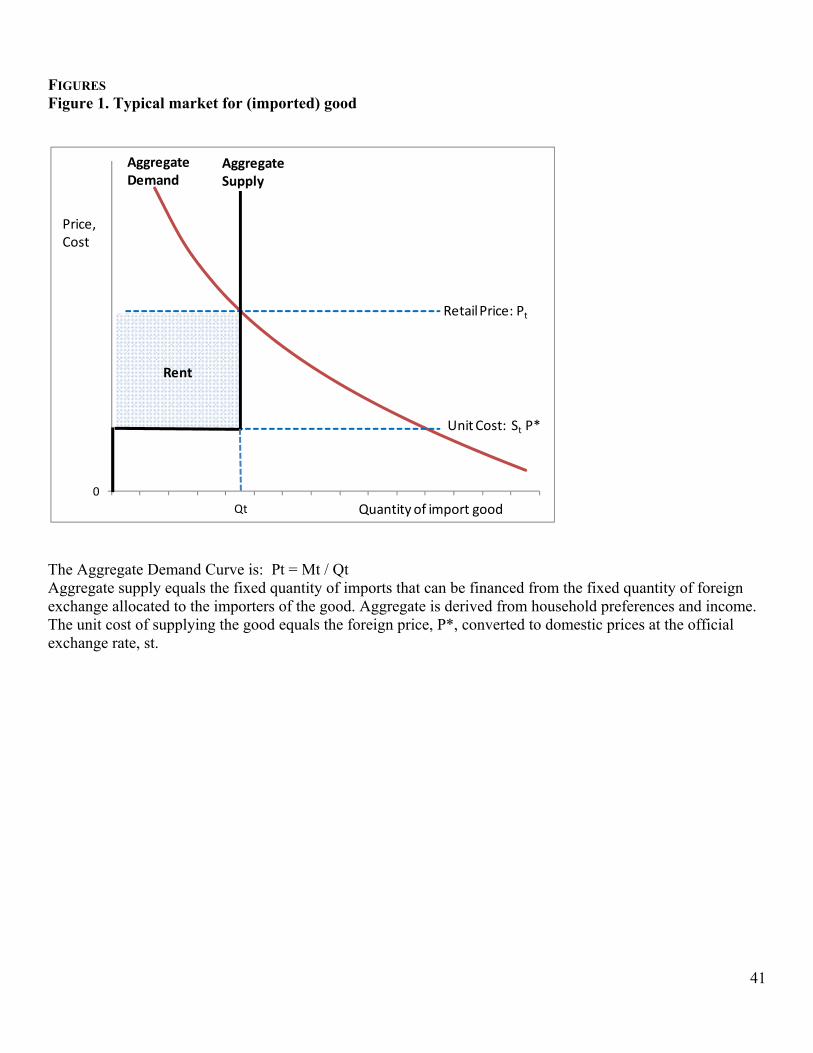
41

FIGURES Figure 1. Typical market for (imported) good

The Aggregate Demand Curve is: Pt = Mt / Qt Aggregate supply equals the fixed quantity of imports that can be financed from the fixed quantity of foreign exchange allocated to the importers of the good. Aggregate is derived from household preferences and income. The unit cost of supplying the good equals the foreign price, P*, converted to domestic prices at the official exchange rate, st.

0

Qt

Rent

Price,Cost

Quantity of import good

Retail Price: Pt

Unit Cost: St P*

Aggregate Demand

AggregateSupply

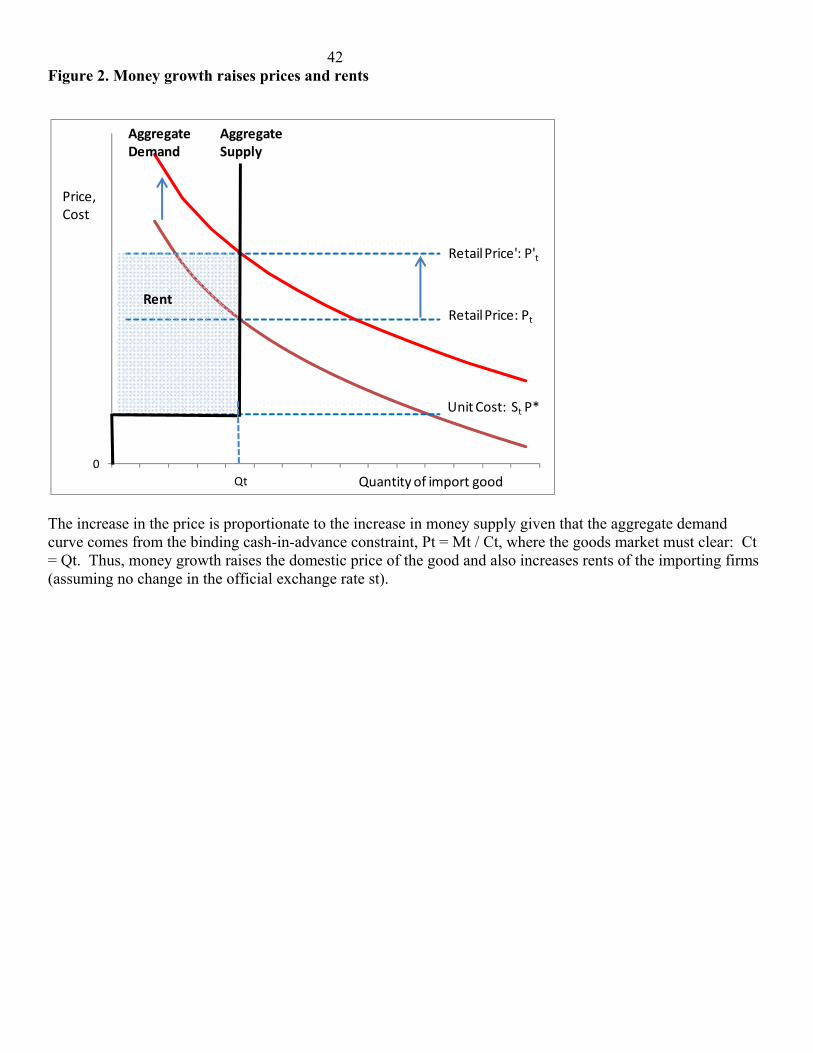
42 Figure 2. Money growth raises prices and rents

The increase in the price is proportionate to the increase in money supply given that the aggregate demand curve comes from the binding cash-in-advance constraint, Pt = Mt / Ct, where the goods market must clear: Ct = Qt. Thus, money growth raises the domestic price of the good and also increases rents of the importing firms (assuming no change in the official exchange rate st).

0

Qt

Rent

Price,Cost

Quantity of import good

Retail Price: Pt

Unit Cost: St P*

Retail Price': P't

Aggregate Demand

Aggregate Supply

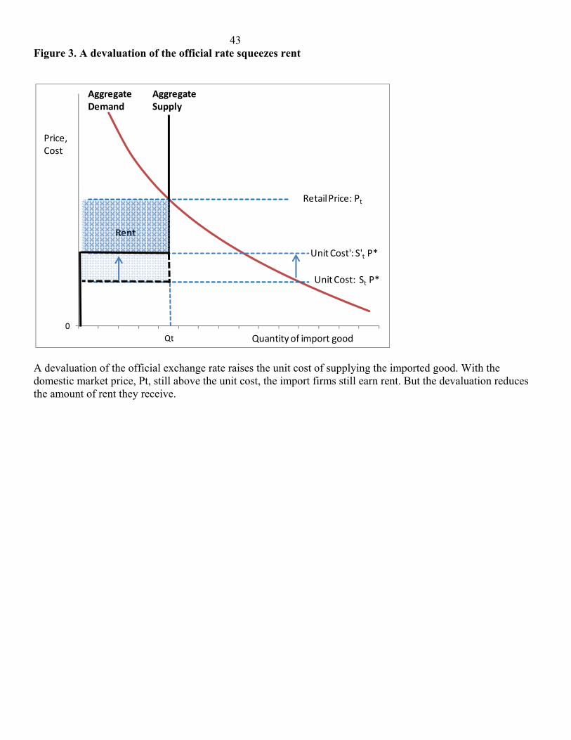
43 Figure 3. A devaluation of the official rate squeezes rent

A devaluation of the official exchange rate raises the unit cost of supplying the imported good. With the domestic market price, Pt, still above the unit cost, the import firms still earn rent. But the devaluation reduces the amount of rent they receive.

0

Qt

Rent

Price,Cost

Quantity of import good

Retail Price: Pt

Unit Cost: St P*

Unit Cost': S't P*

Aggregate Demand

Aggregate Supply

44 Figure 4. Large devaluation to a level above LOOP

If the exchange rate were to be devalued to a level above LOOP (law of one price), there would be an impact on the retail price and the quantity of the good sold. In this case, since the devaluation moves the exchange rate above the level required for LOOP to hold at Qt, there is pass-through of the devaluation to the domestic price level, and there is also import compression.

0

Q't Qt

InitialRent

Price,Cost

Quantity of import good

Retail Price: Pt

Unit Cost: St P*

RetailPrice' = Unit Cost':P't=S't P*

Aggregate Demand

Aggregate Supply

45 Figure 4 (continued). Large devaluation to a level above LOOP

The devaluation increases the domestic value of government revenue from export receipts and reduces the fiscal deficit. There is less need for money creation to finance the fiscal deficit, so the lower money reduces aggregate demand Pt+1 = Mt+1 / Ct+1 = (Mt + Tt - st Xt) / Ct

0

Qt+1 Qt

Price,Cost

Quantity of import good

RetailPrice' = Unit Cost':P't+1=P't=S't P*

Agg Demand Agg SupplyAgg Supply'

46 Figure 5. Oil revenue decline

When oil export receipts decline, the supply of foreign exchange is reduced, which in turn reduces the supply of imported goods. The decline in oil receipts also widens the fiscal deficit, which requires higher money creation and higher aggregate demand. So, the aggregate demand curve increases and the aggregates supply curve contracts, both of which lead to higher inflation.

0

Qt' Qt

Rent

Price,Cost

Quantity of import good

Retail Price: Pt

Unit Cost: St P*

Retail Price': P't

Aggregate Demand

Aggregate Supply

47 Figure 6. Two goods economy

Extending the model to an economy with multiple goods (two in this example), we find that the amount of rents can vary in each of the markets for goods if foreign exchange is allocated in a random (e.g. political, non-economic) way. In the illustration above, suppose that (1-φ) Xt dollars are distributed to import firms in goods markets 1 and 2, which at the international price per unit of P* (let’s assume the same world price for both goods) is used to import quantities Q1 and Q2, respectively. Because very little FX is provided to importers of good 1, the price and rent is higher than in the market for good 2. In addition to the direct allocation of FX to the importing firms, the central bank also sells some of its dollars, φ Xt, to arbitrage firms at the official rate st. In this case, the arbitrage firms would prefer to sell their dollars in the black market to importers of good 1 because the black market price would be higher ( bt = ) due to the higher rents in goods market 1 compared with goods market 2. The sale of dollars to importers of good 1 would also increase the quantity supplied and reduce the price of good 1 somewhat. Thus, in a multiple good economy, the black market rate will tend to reflect the price in the most distorted goods markets (i.e., those with the highest rents or highest relative prices / ∗).

0

Q1 Q1'

Rent

Price,Cost

Quantity of import good

Retail Price: P1t

Unit Cost: St P*

Retail Price': P'1t

Xt / P*

Aggregate Supply'

Aggregate Demand

Aggregate Supply

0

Q2

Rent

Price,Cost

Quantity of import good

Retail Price: P2t

Unit Cost: St P*

Aggregate Demand

Aggregate Supply

48 Figure 7. Price controls and scarcity

is the amount of the good demanded at the controlled price is the fixed supply of the import good, given the FX allocation from export receipts

Price controls reduce the price of the good below the market-clearing free price, and also reduce the rents received by the importing firm. However, at the lower price, there is excess demand for the good, which generates “scarcity” (or shortages in the parlance of economists).

0

Qt Qdt

Rent

Price,Cost

Quantity of import good

FreeRetail Price: Pt

Unit Cost: St P*

Controlled Price: Pc

t

Shortage ("Scarcity")

Aggregate Demand

Aggregate Supply

49 Figure 8. Simulation of an increase in allocation to black market

(Changes from baseline)

-4

-2

0

20

13

20

16

20

19

20

22

Q1t

0

2

4

20

13

20

16

20

19

20

22

Q2t

0

0.5

1

20

13

20

16

20

19

20

22

Mt

0

0.5

1

20

13

20

16

20

19

20

22

st

-50

0

50

100

20

13

20

16

20

19

20

22

-200

0

200

400

20

13

20

16

20

19

20

22

-100

0

100

200

20

13

20

16

20

19

20

22

0

0.5

1

20

13

20

16

20

19

20

22

Tt-stXt (Deficit)

0

0.5

1

20

13

20

16

20

19

20

22

Yt (HHs)

-0.4

-0.2

0.0

20

13

20

16

20

19

20

22

log C1t

0.00.51.01.5

20

13

20

16

20

19

20

22

log C2t

0102030

20

13

20

16

20

19

20

22

P1t/P1*t

-600

-400

-200

0

20

13

20

16

20

19

20

22

P2t/P2*t

-600

-400

-200

0

20

13

20

16

20

19

20

22

bt

-200

0

200

400

20

13

20

16

20

19

20

22

bt/bt-1

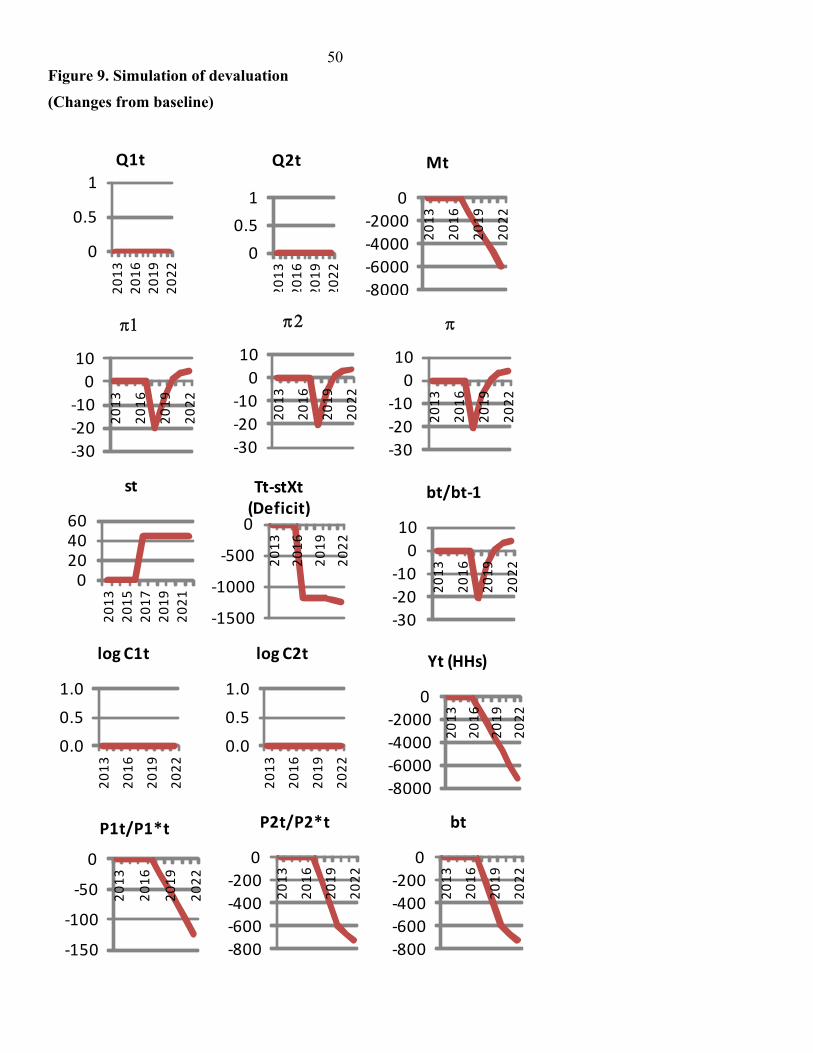
50 Figure 9. Simulation of devaluation

(Changes from baseline)

0

0.5

1

20

13

20

16

20

19

20

22

Q1t

0

0.5

1

20

13

20

16

20

19

20

22

Q2t

-8000

-6000

-4000

-2000

0

20

13

20

16

20

19

20

22

Mt

0204060

20

13

20

15

20

17

20

19

20

21

st

-30

-20

-10

0

10

20

13

20

16

20

19

20

22

-30

-20

-10

0

10

20

13

20

16

20

19

20

22

-30

-20

-10

0

10

20

13

20

16

20

19

20

22

-1500

-1000

-500

0

20

13

20

16

20

19

20

22

Tt-stXt (Deficit)

-8000

-6000

-4000

-2000

0

20

13

20

16

20

19

20

22

Yt (HHs)

0.0

0.5

1.0

20

13

20

16

20

19

20

22

log C1t

0.0

0.5

1.0

20

13

20

16

20

19

20

22

log C2t

-150

-100

-50

0

20

13

20

16

20

19

20

22

P1t/P1*t

-800

-600

-400

-200

0

20

13

20

16

20

19

20

22

P2t/P2*t

-800

-600

-400

-200

0

20

13

20

16

20

19

20

22

bt

-30

-20

-10

0

10

20

13

20

16

20

19

20

22

bt/bt-1

51 Figure 10. Simulation of overinvoicing good 1 to supply good 2

(Changes from baseline)

-1.5

-1

-0.5

0

20

13

20

16

20

19

20

22

Q1t

00.5

11.5

20

13

20

16

20

19

20

22

Q2t

0

0.5

1

20

13

20

16

20

19

20

22

Mt

0

0.5

1

20

13

20

16

20

19

20

22

st

-20

-10

0

10

20

13

20

16

20

19

20

22

-200

-100

0

100

200

20

13

20

16

20

19

20

22

-100

-50

0

50

100

20

13

20

16

20

19

20

22

0

0.5

1

20

13

20

16

20

19

20

22

Tt-stXt (Deficit)

0

0.5

1

20

13

20

16

20

19

20

22

Yt (HHs)

-0.1

0.0

0.0

0.0

20

13

20

16

20

19

20

22

log C1t

0.00.20.40.6

20

13

20

16

20

19

20

22

log C2t

0

1

2

20

13

20

16

20

19

20

22

P1t/P1*t

-300

-200

-100

0

20

13

20

16

20

19

20

22

P2t/P2*t

-300

-200

-100

0

20

13

20

16

20

19

20

22

bt

-200

-100

0

100

200

20

13

20

16

20

19

20

22

bt/bt-1

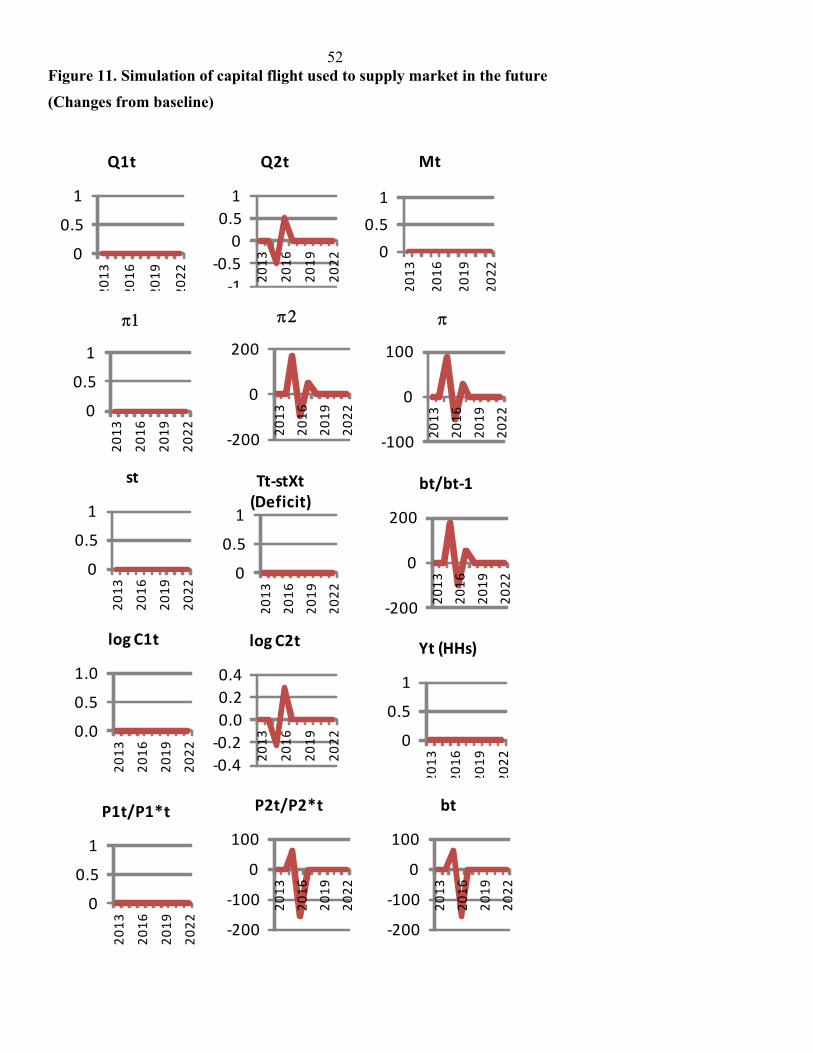
52 Figure 11. Simulation of capital flight used to supply market in the future

(Changes from baseline)

0

0.5

1

20

13

20

16

20

19

20

22

Q1t

-1

-0.5

0

0.5

1

20

13

20

16

20

19

20

22

Q2t

0

0.5

1

20

13

20

16

20

19

20

22

Mt

0

0.5

1

20

13

20

16

20

19

20

22

st

0

0.5

1

20

13

20

16

20

19

20

22

-200

0

200

20

13

20

16

20

19

20

22

-100

0

100

20

13

20

16

20

19

20

22

0

0.5

1

20

13

20

16

20

19

20

22

Tt-stXt (Deficit)

0

0.5

1

20

13

20

16

20

19

20

22

Yt (HHs)

0.0

0.5

1.0

20

13

20

16

20

19

20

22

log C1t

-0.4

-0.2

0.0

0.2

0.4

20

13

20

16

20

19

20

22

log C2t

0

0.5

1

20

13

20

16

20

19

20

22

P1t/P1*t

-200

-100

0

100

20

13

20

16

20

19

20

22

P2t/P2*t

-200

-100

0

100

20

13

20

16

20

19

20

22

bt

-200

0

200

20

13

20

16

20

19

20

22

bt/bt-1