Excel® Pivot TablesStep by Step Guide

www.learnexcelnow.com

C O N Q U E R T H E F E A R O F E X C E L

EXCEL PIVOT TABLES Step by Step Guide

PAGE 2

C O N Q U E R T H E F E A R O F E X C E L

Microsoft® Office Excel® is a registered trademark of the Microsoft Corporation in the United States and other countries. All rights reserved.

Excel Pivot Tables Step by Step Guide

Table of Contents

Intro Page 3Set Up/Build a Pivot Table Page 5Manipulate the Date Page 7Report on the Data Page 9

EXCEL PIVOT TABLES Step by Step Guide

PAGE 3

C O N Q U E R T H E F E A R O F E X C E L

Let’s start with a story….

Zack Smith found his perfect job. As the sales manager for a boutique marketing firm, he had everything he wanted: good salary, easy commute, and a company culture he could get behind.

This is part of the reason he was so stressed out after his first review. The Director of his department wasn’t satisfied with his sales reports. She complained that that data was too unreadable and raw.

She said she expected the reports to be in a Pivot Table from now on. He didn’t know how to create Pivot Tables.

The night after the review he felt frustrated with the job. His confidence waned and be began to dread going into the office the next day.

But with the fresh start of morning he became more optimistic about the job. Before falling asleep the night before, Zack decided was going to wake up and conquer Pivot Tables.

The next time he submitted his reports, he was going to show what he learned…

EXCEL PIVOT TABLES Step by Step Guide

PAGE 4

C O N Q U E R T H E F E A R O F E X C E L

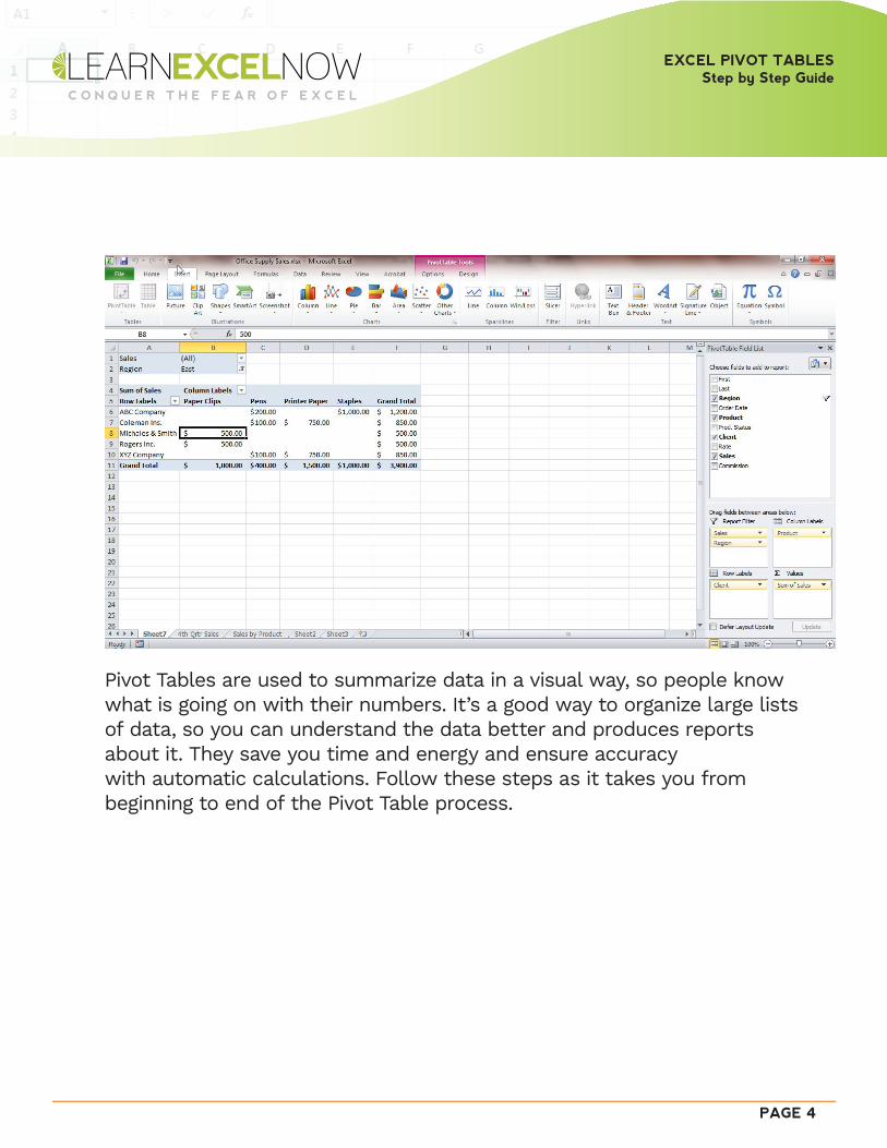
Pivot Tables are used to summarize data in a visual way, so people know what is going on with their numbers. It’s a good way to organize large lists of data, so you can understand the data better and produces reports about it. They save you time and energy and ensure accuracy with automatic calculations. Follow these steps as it takes you from beginning to end of the Pivot Table process.

EXCEL PIVOT TABLES Step by Step Guide

PAGE 5

C O N Q U E R T H E F E A R O F E X C E L

Set Up/Build a Pivot Table

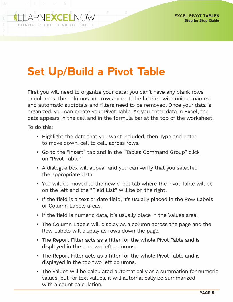
First you will need to organize your data: you can’t have any blank rows or columns, the columns and rows need to be labeled with unique names, and automatic subtotals and filters need to be removed. Once your data is organized, you can create your Pivot Table. As you enter data in Excel, the data appears in the cell and in the formula bar at the top of the worksheet.

To do this:

• Highlight the data that you want included, then Type and enter to move down, cell to cell, across rows.

• Go to the “Insert” tab and in the “Tables Command Group” click on “Pivot Table.”

• A dialogue box will appear and you can verify that you selected the appropriate data.

• You will be moved to the new sheet tab where the Pivot Table will be on the left and the “Field List” will be on the right.

• If the field is a text or date field, it’s usually placed in the Row Labels or Column Labels areas.

• If the field is numeric data, it’s usually place in the Values area.

• The Column Labels will display as a column across the page and the Row Labels will display as rows down the page.

• The Report Filter acts as a filter for the whole Pivot Table and is displayed in the top two left columns.

• The Report Filter acts as a filter for the whole Pivot Table and is displayed in the top two left columns.

• The Values will be calculated automatically as a summation for numeric values, but for text values, it will automatically be summarized with a count calculation.

EXCEL PIVOT TABLES Step by Step Guide

PAGE 6

C O N Q U E R T H E F E A R O F E X C E L

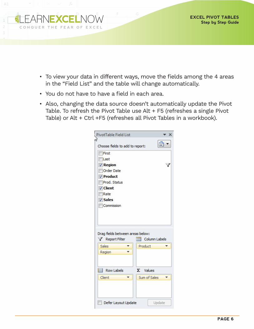
• To view your data in different ways, move the fields among the 4 areas in the “Field List” and the table will change automatically.

• You do not have to have a field in each area.

• Also, changing the data source doesn’t automatically update the Pivot Table. To refresh the Pivot Table use Alt + F5 (refreshes a single Pivot Table) or Alt + Ctrl +F5 (refreshes all Pivot Tables in a workbook).

EXCEL PIVOT TABLES Step by Step Guide

PAGE 7

C O N Q U E R T H E F E A R O F E X C E L

Manipulate the Date

With Pivot Tables, readability is key, so you want to make your data look good. Once you have the Pivot Table structure in place, you can manipulate the data by formatting, sorting, and filtering it. If you want to show less data in the Pivot Table, you can drag a field out of the area section or uncheck it. You can add or remove them as you want.

To format your Pivot Table, right-click on any number and select “Format Cells” and then select the “Number” tab on the left. From there you can set the commas or decimals to make the Pivot Table easier to read. The format you choose will be applied to all the numbers on the Pivot Table.

Sorting data in the Pivot Table can make it easier to understand. Go to the “Options” tab, then click on the “Sort” button. For numeric values, you can sort from largest to smallest or smallest to largest; for text values you can sort alphabetically; and for dates you can sort from oldest to newest or newest to oldest. But, make sure to always double check sorted data to ensure that the information is moving with its source.

EXCEL PIVOT TABLES Step by Step Guide

PAGE 8

C O N Q U E R T H E F E A R O F E X C E L

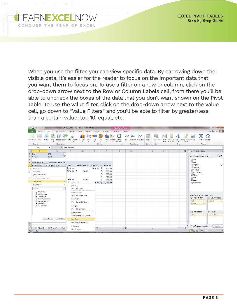
When you use the filter, you can view specific data. By narrowing down the visible data, it’s easier for the reader to focus on the important data that you want them to focus on. To use a filter on a row or column, click on the drop-down arrow next to the Row or Column Labels cell, from there you’ll be able to uncheck the boxes of the data that you don’t want shown on the Pivot Table. To use the value filter, click on the drop-down arrow next to the Value cell, go down to “Value Filters” and you’ll be able to filter by greater/less than a certain value, top 10, equal, etc.

EXCEL PIVOT TABLES Step by Step Guide

PAGE 9

C O N Q U E R T H E F E A R O F E X C E L

Report on the DataWhen reporting data, there are a few options you can choose from including drill down, automatic reports, duplicating Pivot Tables, and Pivot Table web. Sometimes, it might be helpful to drill down into the Pivot Table to show the numbers that make up the summary numbers. To do this, double click on the value that you want to drill down on. Excel will put a duplicate of the source data that was used to create that value on a new worksheet. Another way to do this is to right click on the value and select “Show Details.” If you want to see the details behind the whole Pivot Table, double-click on the “Grand Total” and the data source will be duplicated on a new worksheet.

With automatic reports, a formatted Pivot Table is created on a separate sheet tab for each category of data in the Report Filter area. To do this, click on the “Options” tab, then in the Pivot Table Command Group, click on the “Options” drop-down arrow, and click on “Show Report Filter Pages.” This will create multiple reports automatically.

For reporting, duplicate Pivot Tables can be used to display the data in a combination of different ways. When you copy and paste a Pivot Table, the duplicate holds a copy of the source data, so it can be used to create different views of the data. There are several ways to do this, first highlight the Pivot Table, then right-click and select “Copy” or type “Ctrl” + “C” and the data will be copied. To paste, go to a new worksheet, click on a cell, then right-click and select “Paste” or “Ctrl + “P.” To produce a static copy of the Pivot Table (one that doesn’t hold the source data), when pasting, right-click and select “Paste Special” and choose “Values Only.”

To share your Pivot Table as a web page, go to “File,” then select “Save As.” In the dialog box, under “Save as type” select “Web Page” and click “Publish.”

EXCEL PIVOT TABLES Step by Step Guide

PAGE 10

C O N Q U E R T H E F E A R O F E X C E L

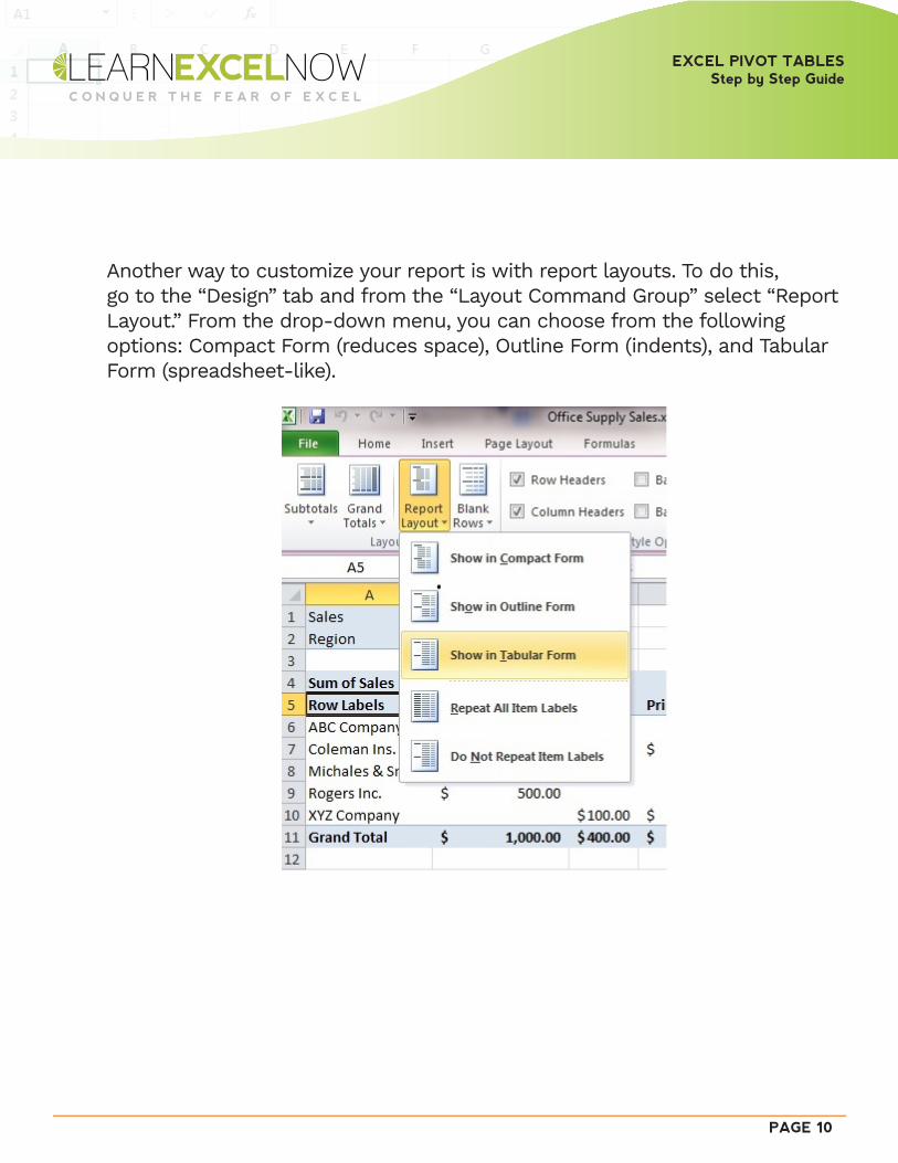
Another way to customize your report is with report layouts. To do this, go to the “Design” tab and from the “Layout Command Group” select “Report Layout.” From the drop-down menu, you can choose from the following options: Compact Form (reduces space), Outline Form (indents), and Tabular Form (spreadsheet-like).

EXCEL PIVOT TABLES Step by Step Guide

PAGE 11

C O N Q U E R T H E F E A R O F E X C E L

We here at Learn Excel Now hope you found this Pivot Table step-by-step guide useful.

If you would like additional information on Excel, please visit us at:

LEARNEXCELNOW.COM

Looking for more training for new users?

Click here to check out our Excel Foundations program

Have questions or want more information? Please email us at: questions@learnexcelnow.com