HAL Id: hal-00426299https://hal.archives-ouvertes.fr/hal-00426299

Submitted on 24 Oct 2009

HAL is a multi-disciplinary open accessarchive for the deposit and dissemination of sci-entific research documents, whether they are pub-lished or not. The documents may come fromteaching and research institutions in France orabroad, or from public or private research centers.

L’archive ouverte pluridisciplinaire HAL, estdestinée au dépôt et à la diffusion de documentsscientifiques de niveau recherche, publiés ou non,émanant des établissements d’enseignement et derecherche français ou étrangers, des laboratoirespublics ou privés.

Estimation of vehicle lateral tire-road forces: acomparison between extended and unscented Kalman

filteringMoustapha Doumiati, Alessandro Victorino, Ali Charara, Daniel Lechner

To cite this version:Moustapha Doumiati, Alessandro Victorino, Ali Charara, Daniel Lechner. Estimation of vehicle lateraltire-road forces: a comparison between extended and unscented Kalman filtering. ECC 09, Aug 2009,Hungary. pp.6, 2009. <hal-00426299>

Estimation of vehicle lateral tire-road forces: a comparison betweenextended and unscented Kalman filtering

Moustapha Doumiati, Alessandro Victorino, Ali Charara andDaniel Lechner

Abstract— Extensive research has shown that most of roadaccidents occur as a result of driver errors. A close examinationof accident data reveals that losing the vehicle control isresponsible for a huge proportion of car accidents. Preventingsuch kind of accidents using vehicle control systems, requirescertain input data concerning vehicle dynamic parametersand vehicle road interaction. Unfortunately, some parameterslike tire-road forces and sideslip angle, which have a majorimpact on vehicle dynamics, are difficult to measure in a car.Therefore, this data must be estimated. Due to the systemnonlinearities and unmodeled dynamics, two observers derivedfrom extended and unscented Kalman filtering techniques areproposed and compared. The estimation process method isbased on the dynamic response of a vehicle instrumentedwith cheap, easily-available standard sensors. Performancesare tested and compared to real experimental data acquiredusing the INRETS-MA Laboratory car. Experimental resultsdemonstrate the ability of this approach to provide accurateestimations, and show its practical potential as a low-costsolution for calculating lateral-tire forces and sideslip angle.

I. I NTRODUCTION

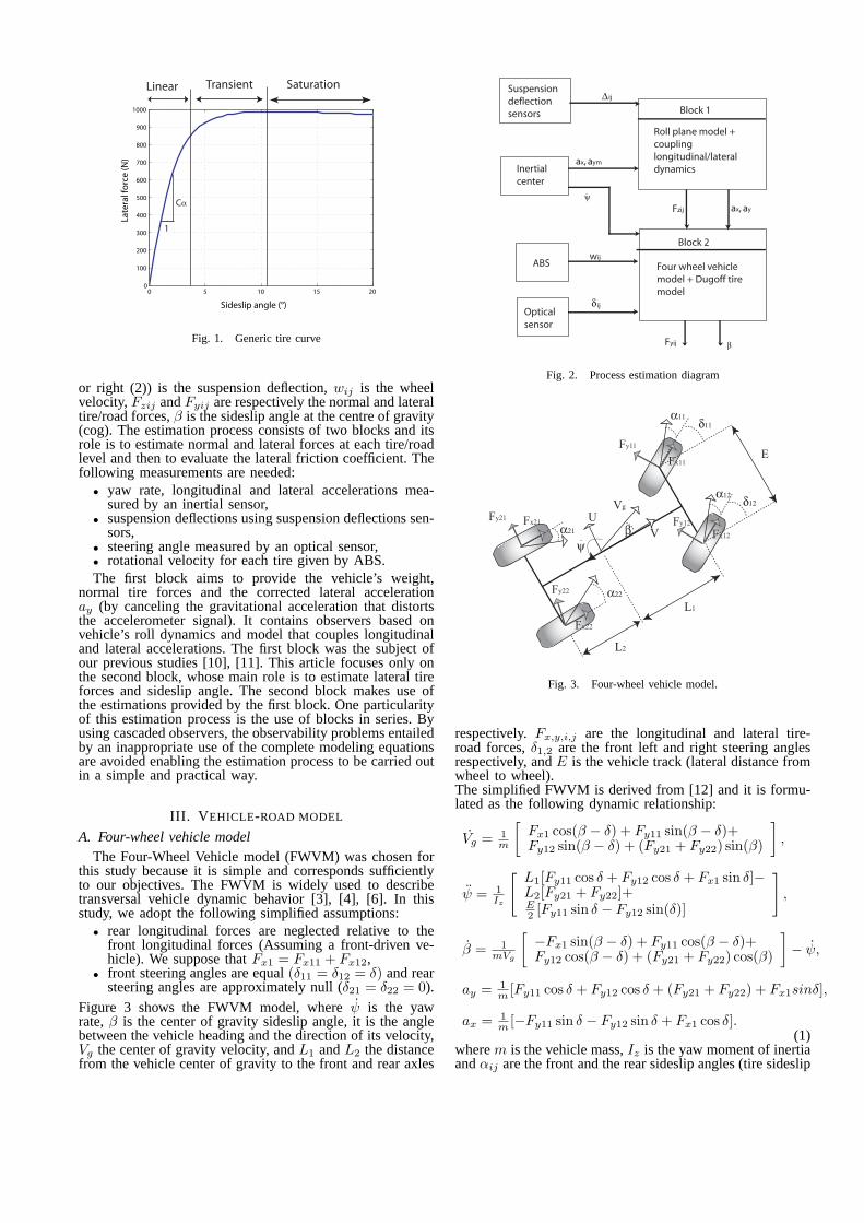
Vehicle control algorithms such as Electronic StabilityControl (ESC) systems have made great strides towardsimproving the handling and safety of vehicles. In fact, expertsestimate that the ESC prevents 27% of loss of control acci-dents by intervening when emergency situations are detected[1]. While ESC is undoubtedly a life-saving technology, itis limited by the available vehicle state information.ESC systems currently available on production cars relyon avaible inexpensive measurements (such as longitudinalvelocity, accelerations and yaw rate), tire model, and sidesliprate, not sideslip angle. Calculating sideslip angle fromsideslip rate integration is prone to uncertainty and errorsfrom sensor biases. Furthermore, other essential parameterslike tire-road forces are difficult to measure because oftechnical, physical and economic reasons. Therefore, theseimportant data must be observed or estimated. If controlsystems could characterize lateral tire forces characteristics,namely lateral forces, sideslip angle and tire-road frictioncoefficient, these systems could greatly enhance vehiclehandling and increase passenger safety.As the motion of a vehicle is governed by the forcesgenerated between the tires and the road, knowledge ofthe tire forces is crucial to predicting vehicle motion. Thelateral forces necessary for a vehicle to hold a curve ariseas a result of tire deformation. As shown in figure 1, therelationship between the lateral force and the slip angle isinitially linear with a constant slope ofCα, referred to asthe cornering stiffness. When operating in the linear region,a vehicle responds predictably to the driver’s inputs. When avehicle undergoes high accelerations, or when road frictionchanges, the vehicle dynamic becomes nonlinear and theforce begins to saturate. Consequently, the tire enters thenonlinear operating region and the vehicle approaches itshandling limits and its response becomes less predictable.

M. Doumiati, A. Victorino and A. Charara are with Heudi-asyc Laboratory, UMR CNRS 6599, Universite de Technologie deCompiegne, 60205 Compiegne, Francemdoumiat@hds.utc.fr,acorreav@hds.utc.fr and acharara@hds.utc.fr

D. Lechner is with Inrets-MA Laboratory, Departement of AccidentMechanism Analysis, Chemin de la Croix Blanche, 13300 Salon deProvence, Francedaniel.lechner@inrets.fr

Lateral vehicle dynamic estimation has been widely dis-cussed in the literature. Several studies have been conductedregarding the estimation of tire-road forces and sideslip angle[2]-[9]. For example, in [2] and [3], the authors estimate thevehicle dynamic state for a four-wheel vehicle model. Con-sequently, tire forces are calculated based on the estimatedstates and using tire models. In [4], Ray estimates the vehicledynamic states and lateral tire forces per axle for a nineDOF vehicle model. The author uses measures of the appliedtorques as inputs to his model. We note that the torque isdifficult to get in practice; it requires expensive sensors.Morerecently, in [5] and [6], authors propose observers to estimatelateral forces per axle without using torque measures. In [7],the authors propose an estimation process based on a threeDOF vehicle model, as a tire force estimator. In [8] and [9],sideslip angle estimation is discussed in details.In [5], [6], [7], lateral forces are modelled with a derivativeequal to random noise. The authors in [7], remark that suchmodeling leads to a noticeable inaccuracy when estimatingindividual lateral tire forces, but not in axle lateral forces.This phenomenon is due to the non-representation of thelateral load transfer when modeling [7].The main goal of this study is to develop an estimationmethod that uses a simple vehicle-road model and a certainnumber of valid measurements in order to estimate accuracyand in real-time the lateral force at each individual tire-road contact point. We suppose a prior knowledge of roadconditions. This study presents two particularities:

• the estimation process does not use the measurement ofwheel torques,

• As described in section II, the estimation process usesaccurate estimated normal tire forces, while other ap-proaches found in the literature assume constant verticalforces.

The observation system is highly nonlinear and presentsunmodeled dynamics. For this reason, two observers basedon EKF (Extended Kalman Filter) and UKF (UnscentedKalman Filter) are proposed. The EKF is probably the mostused estimator for nonlinear systems, however the UKF hasshown the ability to be a superior alternative especially whensystem presents strong nonlinearities. This study comparesand discusses this two filtering techniques in our estimationapproach.In order to show the effectiveness of the estimation method,some validation tests were carried out on an instrumentedvehicle in realistic driving situations.The remainder of the paper is organized as follows. In section2 we describe the estimation process. Section 3 presents thevehicle/road model. Section 4 describes the observer andpresents the observability analysis. In section 5 the observersresults are discussed and compared to real experimental data,and then in the final section we make some concludingremarks regarding our study and future perspectives.

II. ESTIMATION PROCESS DESCRIPTION

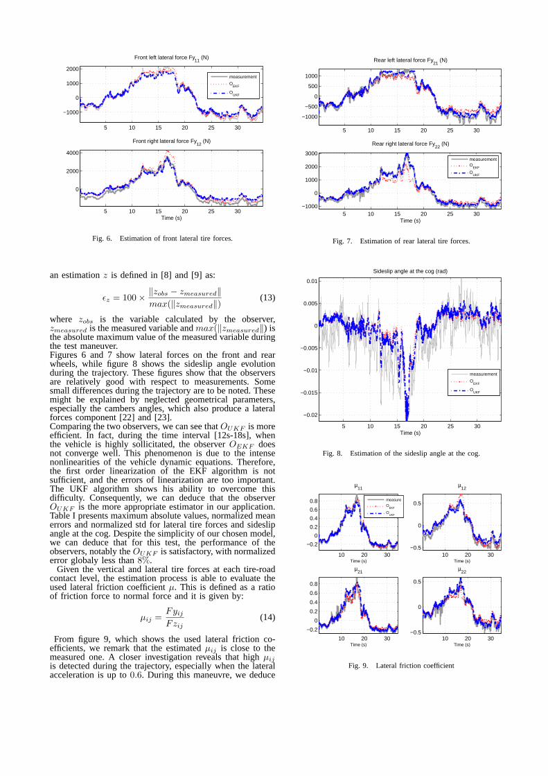
The estimation process is shown in its entirety by theblock diagram in figure 2, whereax andaym are respectivelythe longitudinal and lateral accelerations,ψ is the yaw rate,∆ij ( i represents front(1) or rear(2) andj represents left(1)

0 5 10 15 200

100

200

300

400

500

600

700

800

900

1000

Sideslip angle (°)

La

tera

l fo

rce

(N

)

Linear Transient Saturation

1

Cα

Fig. 1. Generic tire curve

or right (2)) is the suspension deflection,wij is the wheelvelocity,Fzij andFyij are respectively the normal and lateraltire/road forces,β is the sideslip angle at the centre of gravity(cog). The estimation process consists of two blocks and itsrole is to estimate normal and lateral forces at each tire/roadlevel and then to evaluate the lateral friction coefficient.Thefollowing measurements are needed:

• yaw rate, longitudinal and lateral accelerations mea-sured by an inertial sensor,

• suspension deflections using suspension deflections sen-sors,

• steering angle measured by an optical sensor,• rotational velocity for each tire given by ABS.The first block aims to provide the vehicle’s weight,

normal tire forces and the corrected lateral accelerationay (by canceling the gravitational acceleration that distortsthe accelerometer signal). It contains observers based onvehicle’s roll dynamics and model that couples longitudinaland lateral accelerations. The first block was the subject ofour previous studies [10], [11]. This article focuses only onthe second block, whose main role is to estimate lateral tireforces and sideslip angle. The second block makes use ofthe estimations provided by the first block. One particularityof this estimation process is the use of blocks in series. Byusing cascaded observers, the observability problems entailedby an inappropriate use of the complete modeling equationsare avoided enabling the estimation process to be carried outin a simple and practical way.

III. V EHICLE-ROAD MODEL

A. Four-wheel vehicle modelThe Four-Wheel Vehicle model (FWVM) was chosen for

this study because it is simple and corresponds sufficientlyto our objectives. The FWVM is widely used to describetransversal vehicle dynamic behavior [3], [4], [6]. In thisstudy, we adopt the following simplified assumptions:

• rear longitudinal forces are neglected relative to thefront longitudinal forces (Assuming a front-driven ve-hicle). We suppose thatFx1 = Fx11 + Fx12,

• front steering angles are equal(δ11 = δ12 = δ) and rearsteering angles are approximately null (δ21 = δ22 = 0).

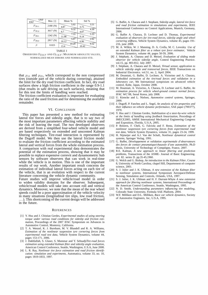
Figure 3 shows the FWVM model, whereψ is the yawrate,β is the center of gravity sideslip angle, it is the anglebetween the vehicle heading and the direction of its velocity,Vg the center of gravity velocity, andL1 andL2 the distancefrom the vehicle center of gravity to the front and rear axles

Suspension

deflection

sensors

Inertial

center

ABS

Optical

sensor

Block 1

Block 2

Roll plane model +

coupling

longitudinal/lateral

dynamics

Four wheel vehicle

model + Dugoff tire

modelδ

ψ

β

∆

.

Fzij

ax, aym

ax, ay

Fyij

ij

wij

ij

Fig. 2. Process estimation diagram

ψ

Vg

β

E

Fy21

Fy22

δ12

Fy11

δ11

L2

L1

Fx11

Fy11

Fx21

Fx22

α11

α12

α21

α22

Fy11

Fx12Fy12

V

U

.

Fig. 3. Four-wheel vehicle model.

respectively.Fx,y,i,j are the longitudinal and lateral tire-road forces,δ1,2 are the front left and right steering anglesrespectively, andE is the vehicle track (lateral distance fromwheel to wheel).The simplified FWVM is derived from [12] and it is formu-lated as the following dynamic relationship:

Vg = 1

m

[

Fx1 cos(β − δ) + Fy11 sin(β − δ)+Fy12 sin(β − δ) + (Fy21 + Fy22) sin(β)

]

,

ψ = 1

Iz

[

L1[Fy11 cos δ + Fy12 cos δ + Fx1 sin δ]−L2[Fy21 + Fy22]+E2[Fy11 sin δ − Fy12 sin(δ)]

]

,

β = 1

mVg

[

−Fx1 sin(β − δ) + Fy11 cos(β − δ)+Fy12 cos(β − δ) + (Fy21 + Fy22) cos(β)

]

− ψ,

ay = 1

m [Fy11 cos δ + Fy12 cos δ + (Fy21 + Fy22) + Fx1sinδ],

ax = 1

m [−Fy11 sin δ − Fy12 sin δ + Fx1 cos δ].(1)

wherem is the vehicle mass,Iz is the yaw moment of inertiaandαij are the front and the rear sideslip angles (tire sideslip

angle is the angle between the tire direction and its velocity).The vehicle velocityVg, the steer angleδ, the yaw rateψand the vehicle body slip angleβ are then used as a basisfor the calculation of the tyre slip anglesαij , where:

α11 = δ − arctan[

Vgβ+L1ψ

Vg−Eψ/2

]

,

α12 = δ − arctan[

Vgβ+L1ψ

Vg+Eψ/2

]

,

α21 = − arctan[

Vgβ−L2ψ

Vg−Eψ/2

]

,

α22 = − arctan[

Vgβ−L2ψ

Vg+Eψ/2

]

.

(2)

B. Lateral tire-force modelThe model of tire-road contact forces is complex because a

wide variety of parameters including environmental factorsand pneumatic properties (load, tire pressure, etc.) impactthe tire-road contact interface. Many different tire modelsare to be found in the literature, based on the physicalnature of the tire and/or on empirical formulations derivingfrom experimental data, such as the Pacejka, Dugoff andBurckhardt models [12], [13]. Dugoff’s model was selectedfor this study because of the small number of parameters thatare sufficient to evaluate the tire-road forces. The nonlinearlateral tire forces are given by:

Fyij = −Cαitanαij .f(λ) (3)

whereCαi is the lateral stiffness,αij is the slip angle andf(λ) is given by:

f(λ) =

{

(2 − λ)λ, if λ < 11, if λ ≥ 1

(4)

λ =µFzij

2Cαi|tanαij |

(5)

In the above formulation,µ is the coefficient of frictionandFzij is the normal load on the tire. This simplified tiremodel assumes no longitudinal forces, a uniform pressuredistribution, a rigid tire carcass, and a constant coefficient offriction of sliding rubber [14].

C. Relaxation modelWhen vehicle sideslip angle changes, a lateral tire force is

created with a time lag. This transient behavior of tires canbe formulated using a relaxation lengthσ. The relaxationlength is the distance covered by the tire while the tire forceis kicking in. Using the relaxation model presented in [15],lateral forces can be written as:

Fyij =Vg

σi(−Fyij + Fyij), (6)

whereFyij is calculated from a Dugoff’s reference tire-forcemodel, Vg is the vehicle velocity andσi is the relaxationlength.

IV. OBSERVER DESIGN

This section presents a description of the observer dedi-cated to lateral tire forces and sideslip angle. The nonlinearstochastic state-space representation of the system describedin the section above is given as:

{

X(t) = f(X(t), U(t)) + bm(t)Y (t) = h(X(t), U(t)) + bs(t)

(7)

The input vectorU comprises the steering angle and thenormal forces considered estimated by the first block (seesection 2):

U = [δ, Fz11, Fz12, , Fz21, Fz22] = [u1, u2, u3, u4, u5].(8)

The measure vector Y(t) comprises yaw rate, vehicle velocity(approximated by the mean of the rear wheel velocitiescalculated from wheel encoders information), longitudinaland lateral accelerations:

Y = [ψ, Vg, ax, ay] = [y1, y2, y3, y4]. (9)

The state vector comprises yaw rate, vehicle velocity, sideslipangle at the cog, lateral forces and the sum of the frontlongitudinal tire forces:

X = [ψ, Vg, β, Fy11, Fy12, Fy21, Fy22, Fx1]= [x1, x2, x3, x4, x5, x6, x7, x8].

(10)The process and measurement noise vectors, respectivelybm(t) and bs(t), are assumed to be white, zero mean anduncorrelated.Consequently, the evolution equations are:

X = f(X,U) = [x1, x2, x3, x4, x5, x6, x7, x8]

x1 = 1

Iz

[

L1[x4 cosu1 + x5 cosu1 + x8 sinu1]−L2[x6 + x7]+E2[x4 sinu1 − x5 sinu1]

]

,

x2 = 1

m

[

x8 cos(x3 − u1) + x4 sin(x3 − u1)+x5 sin(x3 − u1) + (x6 + x7) sin(x3)

]

,

x3 = 1

mVg

[

−x8 sin(x3 − u1) + x4 cos(x3 − u1)+x5 cos(x3 − u1) + (x6 + x7) cosx3

]

− x1,

x4 = x2

σ1

(−x4 + Fy11(α11, u2)),

x5 = x2

σ1

(−x5 + Fy12(α12, u3)),

x6 = x2

σ2

(−x6 + Fy21(α21, u4)),

x7 = x2

σ2

(−x7 + Fy22(α22, u5)),

x8 = 0.(11)

The observation equations are:

y1 = x1,

y2 = x2,

y3 = 1

m [−x4 sinu1 − x5 sinu1 + x8 cosu1],

y4 = 1

m [x4 cosu1 + x5 cosu1 + (x6 + x7) + x6 sinu1].(12)

The state vectorX(t) will be estimated by applying theextended and unscented Kalman filter techniques: observersOEKF andOUKF ) respectively (see section IV-B).

A. ObservabilityObservability is a measure of how well the internal states

of a system can be inferred from knowledge of its inputs andexternal outputs. This property is often presented as a rankcondition on the observability matrix. Using the nonlinearstate space formulation of the system represented in (6), the

Kalman Gain

X=f(X,U)

K

h(X,U) +-

X

Inputs

++evolution

correction

Measurements

observer

sensors

Fig. 4. Process estimation diagram

observability definition is local and uses the Lie derivative[16]. An observability analysis of this system was undertakenin [17]. It has been shown that the system is observableexcept when:

• steering angles are null,• vehicle is at rest (Vg = 0).

For these situations, we assume that lateral forces andsideslip angle are null, which approximately corresponds tothe real cases.

B. Estimation method

The aim of an observer or a virtual sensor is to estimatea particular unmeasurable variable from available measure-ments and a system model in a closed loop observationscheme, as illustrated in figure 4. A simple example of anopen loop observer is the model given by relations (1). Be-cause of the system-model mismatch (unmodelled dynamics,parameter variations,. . . ) and the presence of unknown andunmeasurable disturbances, the calculation obtained fromtheopen loop observer would deviate from the actual values overtime. In order to reduce the estimation error, at least someof the measured outputs are compared to the same variablesestimated by the observer. The difference is fed back into theobserver after being multiplied by a gain matrixK, and so wehave a closed loop observer (see figure 4). The observer wasimplemented in a first-order Euler approximation discreteform. At each iteration, the state vector is first calculatedaccording to the evolution equation and then corrected onlinewith the measurement errors (innovation) and filter gainKin a recursive prediction-correction mechanism. The gain iscalculated using the Kalman filter method which is a set ofmathematical equations and is widely represented in [18],[19].First, theOEKF has been developped in order to estimatethe state vectorX(t) (see section IV). However, some systemproperties and EKF drawbacks encountered during this study,especially:

• the high nonlineaties of the model,• the calculation complexity of the Jacobian matrices

which causes implementation difficulties,

lead us to develop theOUKF . The UKF is introduced toimprove the EKF especially for strong nonlinear systems.For these systems, the first order linearization of the EKFalgorithm using Jacobian matrices is not enough, and theerrors linearization are too important. The UKF acts directlyon the nonlinear model and approximates the states by usinga set of sigma points, avoiding the linearization made by theEKF [20], [21]. The UKF is a powerful nonlinear estimationtechnique and has been shown to be a superior alternative tothe EKF in many robotic applications.

0 200 400 600

0

100

200

300

X position (m)

Y p

ositi

on (

m)

10 20 30

25

26

27

28

Time (s)

Spe

ed (

m.s

1 )

10 20 30

−0.02

0

0.02

0.04

Time(s)

Ste

erin

g an

gle

(rad

)

−0.2 0 0.2 0.4 0.6

−0.1

0

0.1

0.2

Lateral acceleration (g)

Long

itudi

nal a

ccel

erat

ion

(g)

Fig. 5. Experimental test: vehicle trajectory, speed, steering angle andacceleration diagrams

V. EXPERIMENTAL RESULTS

A. Experimental car

The experimental vehicle shown in figure 4 is theINRETS-MA (Institut National de la Recherche sur lesTransports et leur Securite - Departement Mecanismesd’Accidents) Laboratory’s test vehicle. It is a Peugeot 307equipped with a number of sensors including accelerometers,gyrometers, steering angle sensors, linear relative suspen-sion sensors, correvit and dynamometric hubs. Among thesesensors, the correvit (a non-contact optical sensor) givesmeasurements of rear sideslip angle and vehicle velocity,while the dynamometric hubs are wheelforce transducers thatmeasure in real time the forces and moments acting at thewheel center. We note that the correvit and the wheel-forcetransducer are very expensive sensors (correvit: 15 Ke anddynamometric hub: 100 Ke). The sampling frequency of thedifferent sensors is 100Hz.The estimation process algorithm is a computer programwritten in C++. It is integrated into the laboratory car asa DLL (Dynamic Link Library) that functions according tothe software acquisition system.

B. Test conditions

Test data from nominal as well as adverse driving condi-tions were used to assess the performance of the observerpresented in section IV, in realistic driving situations. Wereport a right-left-right bend combination maneuver (one ofa number of experimental tests that we carried out) wherethe dynamic contributions play an important role. Figure 5presents the Peugeot’s trajectory (on a dry road), its speed,steering angle and ”g-g” acceleration diagram during thecourse of the test. The acceleration diagram, that determinesthe maneuvering area utilized by the driver/vehicle, showsthat large lateral accelerations were obtained (absolute valueup to 0.6g). This means that the experimental vehicle wasput in a critical driving situation.

C. Validation of observers

The observer results are presented in two forms: astables of normalized errors, and as figures comparing themeasurements and the estimations. The normalized error for

5 10 15 20 25 30

−1000

0

1000

2000

Front left lateral force Fy11

(N)

5 10 15 20 25 30

0

2000

4000

Time (s)

Front right lateral force Fy12

(N)

measurement

OEKF

OUKF

Fig. 6. Estimation of front lateral tire forces.

an estimationz is defined in [8] and [9] as:

ǫz = 100 ×‖zobs − zmeasured‖

max(‖zmeasured‖)(13)

where zobs is the variable calculated by the observer,zmeasured is the measured variable andmax(‖zmeasured‖) isthe absolute maximum value of the measured variable duringthe test maneuver.Figures 6 and 7 show lateral forces on the front and rearwheels, while figure 8 shows the sideslip angle evolutionduring the trajectory. These figures show that the observersare relatively good with respect to measurements. Somesmall differences during the trajectory are to be noted. Thesemight be explained by neglected geometrical parameters,especially the cambers angles, which also produce a lateralforces component [22] and [23].Comparing the two observers, we can see thatOUKF is moreefficient. In fact, during the time interval [12s-18s], whenthe vehicle is highly sollicitated, the observerOEKF doesnot converge well. This phenomenon is due to the intensenonlinearities of the vehicle dynamic equations. Therefore,the first order linearization of the EKF algorithm is notsufficient, and the errors of linearization are too important.The UKF algorithm shows his ability to overcome thisdifficulty. Consequently, we can deduce that the observerOUKF is the more appropriate estimator in our application.Table I presents maximum absolute values, normalized meanerrors and normalized std for lateral tire forces and sideslipangle at the cog. Despite the simplicity of our chosen model,we can deduce that for this test, the performance of theobservers, notably theOUKF is satisfactory, with normalizederror globaly less than8%.

Given the vertical and lateral tire forces at each tire-roadcontact level, the estimation process is able to evaluate theused lateral friction coefficientµ. This is defined as a ratioof friction force to normal force and it is given by:

µij =Fyij

Fzij(14)

From figure 9, which shows the used lateral friction co-efficients, we remark that the estimatedµij is close to themeasured one. A closer investigation reveals that highµijis detected during the trajectory, especially when the lateralacceleration is up to0.6. During this maneuvre, we deduce

5 10 15 20 25 30

−1000

−500

0

500

1000

Rear left lateral force Fy21

(N)

5 10 15 20 25 30−1000

0

1000

2000

3000

Time (s)

Rear right lateral force Fy22

(N)

measurementO

EKF

OUKF

Fig. 7. Estimation of rear lateral tire forces.

5 10 15 20 25 30

−0.02

−0.015

−0.01

−0.005

0

0.005

0.01

Time (s)

Sideslip angle at the cog (rad)

measurement

OEKF

OUKF

Fig. 8. Estimation of the sideslip angle at the cog.

10 20 30

−0.2

0

0.2

0.4

0.6

0.8

Time (s)

µ11

10 20 30−0.5

0

0.5

Time (s)

µ12

10 20 30

−0.2

0

0.2

0.4

0.6

0.8

Time (s)

µ21

10 20 30−0.5

0

0.5

Time (s)

µ22

measure

OEKF

OUKF

Fig. 9. Lateral friction coefficient

XX

XX

XXEKF

UKF Max ‖‖ Mean % Std %

Fy11 2180 (N)X

XX

XXX

4.875.02 X

XX

XXX

3.753.51

Fy12 3617 (N)X

XX

XXX

9.79.32 X

XX

XXX

4.074.30

Fy21 1342 (N)X

XX

XXX

11.987.55 X

XX

XXX

9.145.33

Fy22 2817 (N)X

XX

XXX

10.125.07 X

XX

XXX

6.962.92

β 0.023X

XX

XXX

13.410.20 X

XX

XXX

10.429.52

TABLE IOBSERVERSOEKF AND OUKF : MAXIMUM ABSOLUTE VALUES ,

NORMALIZED MEAN ERRORS AND NORMALIZED STD.

that µ11 andµ21, which correspond to the non compressedtires (outside part of the vehicle during cornering), attainedthe limit for the dry road friction coefficient. In fact, dry roadsurfaces show a high friction coefficient in the range 0.9-1.1(that results in safe driving on such surfaces), meaning thatfor this test the limits of handling were reached.The friction coefficient evaluation is important for evaluatingthe ratio of the used friction and for determining the availableremainder.

VI. CONCLUSION

This paper has presented a new method for estimatinglateral tire forces and sideslip angle, that is to say two ofthe most important parameters affecting vehicle stabilityandthe risk of leaving the road. The two developed observersare derived from a simplified four-wheel vehicle model andare based respectively on extended and unscented Kalmanfiltering techniques. Tire-road interaction is represented bythe Dugoff model. We then use the lateral friction modelto evaluate the friction coefficient according to the estimatedlateral and vertical forces from the whole estimation process.A comparison with real experimental data demonstrates thepotential of the estimation process, showing that it may bepossible to replace expensive correvit and dynamometric hubsensors by software observers that can work in real-timewhile the vehicle is in motion. This is one of the importantresults of our work. Another important result concerns theestimation of individual lateral forces acting on each tireofthe vehicle, that is an evolution with respect to the currentliterature concerning the vehicle dynamic community.Future studies will improve vehicle/road model in orderto widen validity domains for the observer. Subsequent,vehicle/road models will take into account roll and verticaldynamics. Moreover, we note that the mean of the rear wheelspeeds could be a poor approximation of the vehicle velocityin many situations (longitudinal tire slips, low road friction,. . . ). This shortcoming of the current design will be addressedin the future.

REFERENCES

[1] Y. Hsu and J. Chistian Gerdes,Experimental studies of using steeringtorque under various road conditions for sideslip and friction esti-mation, Proceedings of the 2007 IFAC Symposium on Advances inAutomotive Control, Monterey, California.

[2] T. A. Wenzel, K. J. Burnham, M. V. Blundell and R. A. Williams,Estimation of the nonlinear suspension tyre cornering forces fromexperimental road test data, Vehicle System Dynamics, volume 44,pages 153-171, 2006.

[3] J. Dakhlallah, S. Glaser, S. Mammar and Y. SebsadjiTire-road forcesestimation using extended Kalman filter and sideslip angle evaluation,American Control Conference, Seattle, Washington, U.S.A, June 2008.

[4] L. R. Ray, Nonlinear tire force estimation and road friction identifi-cation: simulation and experiments, Automatica, volume 33, no. 10,pages 1819-1833, 1997.

[5] G. Baffet, A. Charara and J. Stephant,Sideslip angle, lateral tire forceand road friction estimation in simulations and experiments, IEEEInternational Conference on Control Applications, Munich, Germany,2006.

[6] G. Baffet A. Charara, D. Lechner and D. Thomas,Experimentalevaluation of observers for tire-road forces, sideslip angle and wheelcornering stiffness, Vehicle System Dynamics, volume 45, pages 191-216, june 2008.

[7] M. A. Wilkin, W. J. Manning, D. A. Crolla, M. C. LevesleyUse ofan extended Kalman filter as a robust tyre force estimator, VehicleSystem Dynamics, volume 44, pages 50-59, 2006.

[8] J. Stephant, A. Charara and D. Meizel,Evaluation of sliding modeobserver for vehicle sideslip angle, Control Engineering Practice.vol.15, pp. 803-812, July 2007.

[9] J. Stephant, A. Charara and D. Meizel,Virtual sensor, application tovehicle sideslip angle and transversal forces, IEEE Transactions onIndustrial Electronics. vol.51, no. 2, April 2004.

[10] M. Doumiati, G. Baffet, D. Lechner, A. Victorino and A. Charara,Embedded estimation of the tire/road forces and validationin alaboratory car, 9th International symposium on advanced vehiclecontrol, Kobe, Japan, Octobre 2008.

[11] M. Doumiati, A. Victorino, A. Charara, D. Lechner and G. Baffet, Anestimation process for vehicle wheel-ground contact normal forces,IFAC WC’08, Seoul Korea, july 2008.

[12] U. Kiencke and L. Nielsen,Automotive control systems, Springer,2000.

[13] J. Dugoff, P. Fanches and L. Segel,An analysis of tire properties andtheir influence on vehicle dynamic performance, SAE paper (700377),1970.

[14] Y. Hsu and J. Chistian Gerdes,Stabilization of a steer-by-wire vehicleat the limits of handling using feedback linearization, Procedings ofIMECE2005, AMSE International Mechanical Engineering Congressand Exposition, Florida, U.S.A, 2005.

[15] P. Bolzern, F. Cheli, G. Falciola and F. Resta,Estimation of thenonlinear suspension tyre cornering forces from experimental roadtest data, Vehicle System Dynamics, volume 31, pages 23-24, 1999.

[16] H. Nijmeijer and A.J. Van der Schaft,Nonlinear dynamical controlsystems, Springer Verlag, 1991.

[17] G. Baffet, Developpement et validation exprimentale d’observateursdes forces de contact pneumatique/chaussee d’une automobile, Ph.Dthesis, University of Technology of Compiegne, France, 2007.

[18] R.E. Kalman, A new approach to linear filtering and predictionproblems, Transactions of the ASME- Journal of Basic Engineering.vol. 82. series D. pp.35-45,1960.

[19] G. Welch and G. Bishop,An introduction to the Kalman Filter, Course8, University of North Carolina, chapel Hill, Departement ofcomputerscience, 2001.

[20] S. J. Julier and J. K. Uhlman,A new extension of the Kalman filterto nonlinear systems, International Symposium Aerospace/DefenseSensing, Simulation and Controls, Orlando, USA, 1997.

[21] S. J. Julier, J. K. Uhlman and H. F. Durrant-WhyteA new extensionapproach for filtering nonlinear systems, International Proceedings ofthe American Control Conference, Seattle, Washington, 1995.

[22] N. D. Smith, Understanding parameters influencing tire modeling,Colorado State University, Formula SAE Platform, 2004.

[23] W.F. Milliken and D.L. Milliken, Race car vehicle dynamics, Societyof Automotive Engineers, Inc, U.S.A, 1995.