1

DETERMINATION OF PRYING LOAD ON BOLTED CONNECTIONS

A THESIS SUBMITTED TOTHE GRADUATE SCHOOL OF NATURAL AND APPLIED SCIENCES

OFMIDDLE EAST TECHNICAL UNIVERSITY

BY

MERT ATASOY

IN PARTIAL FULFILLMENT OF THE REQUIREMENTSFOR

THE DEGREE OF MASTER OF SCIENCEIN

AEROSPACE ENGINEERING

FEBRUARY 2012

Approval of the thesis:

DETERMINATION OF PRYING LOAD ON BOLTED CONNECTIONS

submitted by MERT ATASOY in partial fulfillment of the requirements for the degree ofMaster of Science in Aerospace Engineering Department, Middle East Technical Uni-versity by,

Prof. Dr. Canan OZGENDean, Graduate School of Natural and Applied Sciences

Prof. Dr. Ozan TEKINALPHead of Department, Aerospace Engineering

Prof. Dr. Altan KAYRANSupervisor, Aerospace Engineering Dept., METU

Examining Committee Members:

Assist. Prof. Dr. Demirkan COKERAerospace Engineering Dept. , METU

Prof. Dr. Altan KAYRANAerospace Engineering Dept. , METU

Assist. Prof. Dr. Melin SAHINAerospace Engineering Dept. , METU

Assist. Prof. Dr. Ercan GURSESAerospace Engineering Dept. , METU

M.Sc. Cem GENCREHIS-SMD , ASELSAN

Date:

I hereby declare that all information in this document has been obtained and presentedin accordance with academic rules and ethical conduct. I also declare that, as requiredby these rules and conduct, I have fully cited and referenced all material and results thatare not original to this work.

Name, Last Name: MERT ATASOY

Signature :

iii

ABSTRACT

DETERMINATION OF PRYING LOAD ON BOLTED CONNECTIONS

ATASOY, Mert

M.Sc., Department of Aerospace Engineering

Supervisor : Prof. Dr. Altan KAYRAN

February 2012, 114 pages

Analysis of aircraft structures are mainly performed by assuming that the structure behaves

linearly. In linear finite element analysis, it is assumed that deformations are small, thus

geometric nonlinearity can be neglected. In addition, linear analysis assumes that linear con-

stitutive laws applicable, implying that material nonlinearity can also be neglected. One very

common type of nonlinearity is associated with the boundary conditions. Contact between

two deformable bodies or between a deformable and rigid body are typical examples of non-

linearity associated with boundary conditions. Linear structural analysis, in general, does

not include contact analysis. Simplicity of linear analysis in terms modeling, interpreting the

results and solution time makes the linear analysis approach very convenient in preliminary

design and analysis stage of aircraft structures. However, simplicity of linear analysis may

result in unconservative results which may occur due to neglecting the true nonlinear behav-

ior of the structure. In this thesis, one such nonlinear effect called prying load effect on the

tensile connections is studied. The effect of prying load on structures are initially described

by referencing the analytical approaches presented in the literature. Finite element models of

typical bolted connections such as L and T type are generated for various combinations of the

chosen design parameters such as bolt diameter, flange thickness, washer diameter and edge

distances. Parametric modeling approach is used to perform the high number of finite element

iv

analysis which involve contact for the purpose of calculating the prying load. Comparative

study of the effect of prying load is then conducted by also including the results presented

in the literature. Comparisons of the prying load are done with the experimental results pre-

sented in the literature. Series of finite element analyses are preformed for various cases such

that effect of geometrical variables and bolt preload on prying ratio can be understood. Ac-

cording to the results obtained, it is concluded that main factors effecting the prying ratio are

the distance of bolt center to the clip web, flange thickness of the clip and preload on the bolt

where the effect of edge distance of the bolt is insignificant.

Keywords: Prying Effect, Prying Load, Finite Element Method, Tensile Connection

v

OZ

CIVATALI BAGLANTILARDA KANIRTMA KUVVETININ BELIRLENMESI

ATASOY, Mert

Yuksek Lisans, Havacılık ve Uzay Muhendisligi Bolumu

Tez Yoneticisi : Prof. Dr. Altan KAYRAN

Subat 2012, 114 sayfa

Havacılık yapılarının analizleri temel olarak dogrusallık varsayımıyla yapılır. Dogrusal sonlu

eleman analizlerinde yer degistirmeler kucuk kabul edilir dolayısıyla geometrik acıdan dogru-

sal olmama durumu goz ardı edilir. Ek olarak, dogrusal analizlerde temel kurallar uygulan-

abilinir kabul edilirken, malzemenin dogrusal olmadıgı durumlar gozardı edilebilir. Iki ya-

mulgan ya da bir yamulgan ve bir esnemez yapı arasında tanımlanan temas dogrusal olmayan

durumların sınır kosulları ile olusmasına verilecek tipik orneklerdir. Dogrusal yapısal analiz

genelde temas ozelligini icermez. Dogrusal analizlerin modellemedeki basitligi sonucların

alınması ve cozum surelerinin kısa olması nedeniyle havacılık yapılarının oncul tasarımlarının

ve analizlerinin yapılması acısından cok kullanıslıdır. Ote yandan, dogrusal analizlerin ba-

sitligi yapının gercekte dogrusal olmayan tavrını goz ardı ettigi icin kimi zaman azımsanmıs

sonuclar sunabilir. Bu tezde bir dogrusal olmama durumu olan kanırtma kuvvetinin cekme

gerilmeli baglantılardaki etkileri incelenmistir. Bu etkiler oncelikle kaynaklara atıflarla sunul-

mustur. L ve T kesitli, civatalı baglantıların sonlu eleman modelleri, secilmis olan civata capı,

ayak kalınlıgı, pul capı ve kenara uzaklık gibi tasarım degiskenlerinin olusturdugu cok sayıda

duzen icin yaratılmıstır. Kanırtma kuvvetinin hesaplanabilmesi icin degistirgesel modelleme

yaklasımı ile bu temas tanımını iceren cok sayıdaki model analiz edilmistir. Kaynaklarda ve-

rilen sonucların da dahil edildigi kanırtma kuvveti karsılastırmaları yapılmıstır. Kaynaklarda

vi

yer alan deneysel kanırtma kuvveti olcum sonuclarıyla da karsılastırmalar yapılmıstır. Bir-

birinden farklı geometrik ozelliklerdeki baglantılar icin bir dizi sonlu elemanlar yontemine

dayalı analiz gerceklestirilerek kanırtma oranını etkileyen geometrik degiskenler ve civatanın

on geriliminin etkisi anlasılmaya calısılmıstır. Edinilen sonuclara gore, kanırtma oranını asıl

etkileyen etmenler civatanın flanj kokune olan uzaklıgı, flanj kalınlıgı ve civata uzerindeki

ongerdirme olarak belirlenmistir. Civatanın flanj kenarına olan uzaklıgı kanırtma oranı uzerin-

de etkisiz bulunmustur.

Anahtar Kelimeler: Kanırtma Etkisi, Kanırtma Yuku, Sonlu Elemanlar Yontemi, Cekme

Baglantısı

vii

To My Love

viii

ACKNOWLEDGMENTS

First of all, I would like to thank to my family for supporting and trusting me all my life. I

surely owe them much more than this work.

I would like to express my gratitude to Prof. Dr. Altan Kayran for guiding this work. His

afford on this thesis is incomparable.

I should not forget to thank to Edip Sirin for helping me to discover the subject of this thesis.

His guidance let me to understand the engineering point of view and so brought me more

confidence on this work and many others.

Thanks to Mustafa Ekren for guiding me to decide where to start, and sharing me his experi-

ence.

All staff of BiAS Engineering starting from Sedat Ozozturk, deserve to be acknowledged

for sharing those beautiful times and experience. There is no better solution of any kind of

confusion rather than talking with Sedat for a while.

Special thanks to dear friend Mehmet Burak Sayar for his guidance to find very critical short-

cuts on modeling and for sharing his energy to overcome difficulties throughout our friend-

ship.

Thanks to my colleagues and managers at ASELSAN for sustaining sleepy me, after long

study nights.

And very special thanks to sweet Cigdem Aysenur Safak for her endless support and love.

ix

TABLE OF CONTENTS

ABSTRACT . . . . . . . . . . . . . . . . . . . . . . . . . . . . . . . . . . . . . . . . iv

OZ . . . . . . . . . . . . . . . . . . . . . . . . . . . . . . . . . . . . . . . . . . . . . vi

ACKNOWLEDGMENTS . . . . . . . . . . . . . . . . . . . . . . . . . . . . . . . . . ix

TABLE OF CONTENTS . . . . . . . . . . . . . . . . . . . . . . . . . . . . . . . . . x

LIST OF TABLES . . . . . . . . . . . . . . . . . . . . . . . . . . . . . . . . . . . . xiii

LIST OF FIGURES . . . . . . . . . . . . . . . . . . . . . . . . . . . . . . . . . . . . xiv

LIST OF ABBREVIATIONS . . . . . . . . . . . . . . . . . . . . . . . . . . . . . . . xviii

CHAPTERS

1 INTRODUCTION . . . . . . . . . . . . . . . . . . . . . . . . . . . . . . . 1

1.1 Objective of The Thesis . . . . . . . . . . . . . . . . . . . . . . . . 1

1.2 Background . . . . . . . . . . . . . . . . . . . . . . . . . . . . . . 2

1.2.1 Aircraft Structures and Prying Effect . . . . . . . . . . . . 2

1.2.2 Analysis of Connections Exposed to Prying Effect . . . . . 5

1.3 Literature Review . . . . . . . . . . . . . . . . . . . . . . . . . . . 6

1.4 Structure of The Thesis . . . . . . . . . . . . . . . . . . . . . . . . 12

2 ANALYTICAL STUDY . . . . . . . . . . . . . . . . . . . . . . . . . . . . 13

2.1 Behavior of the Tension Clip Connections . . . . . . . . . . . . . . 13

2.2 Prying Load Calculation Approaches of Bruhn and Niu . . . . . . . 19

2.3 Douty and McGuire’s Method . . . . . . . . . . . . . . . . . . . . . 20

2.4 Agerskov’s Method . . . . . . . . . . . . . . . . . . . . . . . . . . 22

2.5 Struik and de Back’s Method . . . . . . . . . . . . . . . . . . . . . 26

2.6 Design Considerations in terms of Prying Effect . . . . . . . . . . . 28

3 FINITE ELEMENT MODELING . . . . . . . . . . . . . . . . . . . . . . . 31

x

3.1 Mesh Description . . . . . . . . . . . . . . . . . . . . . . . . . . . 31

3.2 Boundary Conditions and Loads . . . . . . . . . . . . . . . . . . . 33

3.3 Contact Definitions . . . . . . . . . . . . . . . . . . . . . . . . . . 38

3.4 Material Properties . . . . . . . . . . . . . . . . . . . . . . . . . . . 39

3.5 Analysis Steps and Obtaining Prying Load Data . . . . . . . . . . . 39

3.6 Mesh Convergence Study . . . . . . . . . . . . . . . . . . . . . . . 41

3.7 Parametric Modeling . . . . . . . . . . . . . . . . . . . . . . . . . 43

3.8 Description of the Phyton Scripting . . . . . . . . . . . . . . . . . . 44

4 COMPARISON STUDY WITH THE EXPERIMENTS . . . . . . . . . . . . 47

4.1 Comparison with Agerskov’s Study . . . . . . . . . . . . . . . . . . 47

4.2 Modeling of Agerskov’s Test Structures . . . . . . . . . . . . . . . 47

4.3 Comparison of Results . . . . . . . . . . . . . . . . . . . . . . . . . 49

5 PARAMETRIC STUDY . . . . . . . . . . . . . . . . . . . . . . . . . . . . 52

5.1 Factors Affecting the Prying Load Ratio . . . . . . . . . . . . . . . 52

5.2 Effect of Applied Load . . . . . . . . . . . . . . . . . . . . . . . . 53

5.3 Effect of (a) and (b) and Their Ratio (b/a) on the Prying Load . . . . 55

5.4 The Effect of Flange Thickness on the Prying Ratio . . . . . . . . . 61

5.5 The Effect of Preload on the Prying Ratio . . . . . . . . . . . . . . . 63

6 DISCUSSIONS AND CONCLUSIONS . . . . . . . . . . . . . . . . . . . . 68

REFERENCES . . . . . . . . . . . . . . . . . . . . . . . . . . . . . . . . . . . . . . 72

APPENDICES

A PHYTON SCRIPTING . . . . . . . . . . . . . . . . . . . . . . . . . . . . . 74

A.1 Suggestions for Phyton Scripting on Abaqus . . . . . . . . . . . . . 74

A.2 Script Used for Parametric Study . . . . . . . . . . . . . . . . . . . 74

B AGERSKOV TEST SPECIMENS . . . . . . . . . . . . . . . . . . . . . . . 88

B.1 Properties of Test Specimens Used by Agerskov . . . . . . . . . . . 88

C ALLOWABLE LOAD GRAPHICS FOR TENSILE CONNECTIONS . . . . 90

C.1 Graphics presented by Bruhn . . . . . . . . . . . . . . . . . . . . . 90

C.2 Graphics presented by Niu . . . . . . . . . . . . . . . . . . . . . . . 93

C.3 Graphics of ESDU 84039 . . . . . . . . . . . . . . . . . . . . . . . 96

xi

D MATERIAL PROPERTIES and BOLT SPECIFICATIONS . . . . . . . . . . 98

D.1 AISI300 . . . . . . . . . . . . . . . . . . . . . . . . . . . . . . . . 98

D.2 AL2024 . . . . . . . . . . . . . . . . . . . . . . . . . . . . . . . . 99

D.3 NAS609 . . . . . . . . . . . . . . . . . . . . . . . . . . . . . . . . 100

E SIMULATION MODELS PREPARED by PARAMETRIC STUDY and COM-PLETE RESULTS . . . . . . . . . . . . . . . . . . . . . . . . . . . . . . . 101

E.1 Code Generated for the Description Models . . . . . . . . . . . . . 101

E.2 Complete Results in Table Format . . . . . . . . . . . . . . . . . . . 102

F MEDIAL AXES MESHING ALGORITHM . . . . . . . . . . . . . . . . . . 114

xii

LIST OF TABLES

TABLES

Table 4.1 Comparison of Bolt Forces [1] . . . . . . . . . . . . . . . . . . . . . . . . 49

Table 5.1 Data Set Used for the Parametric Study . . . . . . . . . . . . . . . . . . . . 53

Table B.1 Dimension and Mechanical Properties of Test Specimens [1] . . . . . . . . 89

Table E.1 Complete Q/F Results of Finite Element Analyses . . . . . . . . . . . . . 102

xiii

LIST OF FIGURES

FIGURES

Figure 1.1 Prying Load on Angle Section . . . . . . . . . . . . . . . . . . . . . . . . 3

Figure 1.2 Tension Clips Connecting Frames . . . . . . . . . . . . . . . . . . . . . . 3

Figure 1.3 Aircraft Fuselage Assembly and Shear-Clip Connections . . . . . . . . . . 4

Figure 1.4 Prying Effect Representation from Bruhn [6] . . . . . . . . . . . . . . . . 6

Figure 1.5 Tension Clip Design Considerations of Bruhn[6] . . . . . . . . . . . . . . 7

Figure 1.6 Formed and Extruded Sections[7] . . . . . . . . . . . . . . . . . . . . . . 7

Figure 1.7 Fastener Installation for Clip Connections [7] . . . . . . . . . . . . . . . . 8

Figure 1.8 Prying Load Distribution by Niu[7] . . . . . . . . . . . . . . . . . . . . . 9

Figure 2.1 Free Body Diagram of the Angle Section . . . . . . . . . . . . . . . . . . 13

Figure 2.2 T Section Overall Free Body Diagram . . . . . . . . . . . . . . . . . . . . 15

Figure 2.3 T Section Free Body Diagrams . . . . . . . . . . . . . . . . . . . . . . . 15

Figure 2.4 Bolt Force Variation Due to Applied External Load on Preloaded Bolt [2] . 17

Figure 2.5 Effect of Prying on Bolt Force Variation [2] . . . . . . . . . . . . . . . . . 18

Figure 2.6 Actual Effect of Prying on Bolt Force Variation [21] . . . . . . . . . . . . 18

Figure 2.7 Bending moments acting on flange[22] . . . . . . . . . . . . . . . . . . . 19

Figure 2.8 Simplified Prying Model of Douty and McGuire [3] . . . . . . . . . . . . 20

Figure 2.9 Prying Model of Agerskov [1] . . . . . . . . . . . . . . . . . . . . . . . . 23

Figure 2.10 Detailed Bolt Model of Agerskov [1] . . . . . . . . . . . . . . . . . . . . 24

Figure 2.11 Prying Model of Struik and de Back [2] . . . . . . . . . . . . . . . . . . . 26

Figure 2.12 Struik Model with Bolt Head Force and Internal Moment Distribution on

Flange [11] . . . . . . . . . . . . . . . . . . . . . . . . . . . . . . . . . . . . . . 27

Figure 2.13 Effective Flange Length for Bending [9] . . . . . . . . . . . . . . . . . . . 30

xiv

Figure 3.1 3D Clip Model . . . . . . . . . . . . . . . . . . . . . . . . . . . . . . . . 32

Figure 3.2 3D Bolt Model . . . . . . . . . . . . . . . . . . . . . . . . . . . . . . . . 32

Figure 3.3 Complete View of 3D Model of Bolted Clip Connection . . . . . . . . . . 33

Figure 3.4 Boundary Conditions Applied on Side Faces . . . . . . . . . . . . . . . . 34

Figure 3.5 Sectional View of Tension Clip Connection . . . . . . . . . . . . . . . . . 34

Figure 3.6 Boundary Condition Applied on Top Surface . . . . . . . . . . . . . . . . 35

Figure 3.7 Symmetry Boundary Condition Applied on Back Surface of the Clip Web . 36

Figure 3.8 Boundary Condition Applied on the Bolt . . . . . . . . . . . . . . . . . . 36

Figure 3.9 Preload Application on Bolt . . . . . . . . . . . . . . . . . . . . . . . . . 37

Figure 3.10 External Load Application on Top Surface . . . . . . . . . . . . . . . . . 37

Figure 3.11 Contact Regions Defined on Bolted Clip Model . . . . . . . . . . . . . . . 38

Figure 3.12 Step 1 - Initializing Boundary Conditions and Contacts . . . . . . . . . . . 39

Figure 3.13 Step 2 - Activating the Preload . . . . . . . . . . . . . . . . . . . . . . . . 40

Figure 3.14 Step 3 - Deactivating the Constraint on the Corner Node . . . . . . . . . . 40

Figure 3.15 Step 4 - Applying External Load . . . . . . . . . . . . . . . . . . . . . . . 41

Figure 3.16 Element Size Sensitivity Study in terms of Prying Ratio . . . . . . . . . . 42

Figure 3.17 Element Size Sensitivity Study in terms of Process Duration . . . . . . . . 42

Figure 3.18 Parametric Dimensions of Angle Sections with Single Bolt . . . . . . . . . 43

Figure 3.19 Parametric Dimensions of Angle Sections - Upper View . . . . . . . . . . 44

Figure 3.20 Parametric Modeling Script - Main Algorithm Diagram . . . . . . . . . . 45

Figure 3.21 (*)Part Modeling Algorithm Diagram . . . . . . . . . . . . . . . . . . . . 46

Figure 4.1 Comparison of Bolt Forces; Correlation Between Theory and Analysis . . 50

Figure 4.2 Comparison of Bolt Forces; Correlation Between Test and Analysis . . . . 51

Figure 5.1 Effect of Applied Load on the Prying Ratio . . . . . . . . . . . . . . . . . 54

Figure 5.2 Effect of a/D on Prying Ratio for Different Bolt Diameters . . . . . . . . . 55

Figure 5.3 Effect of b on Prying Ratio for Various Diameters for L Sections . . . . . . 56

Figure 5.4 Effect of b on Prying Ratio for Various Diameters for T Sections . . . . . . 56

Figure 5.5 Effect of b/a on Prying Ratio for L Sections . . . . . . . . . . . . . . . . 58

xv

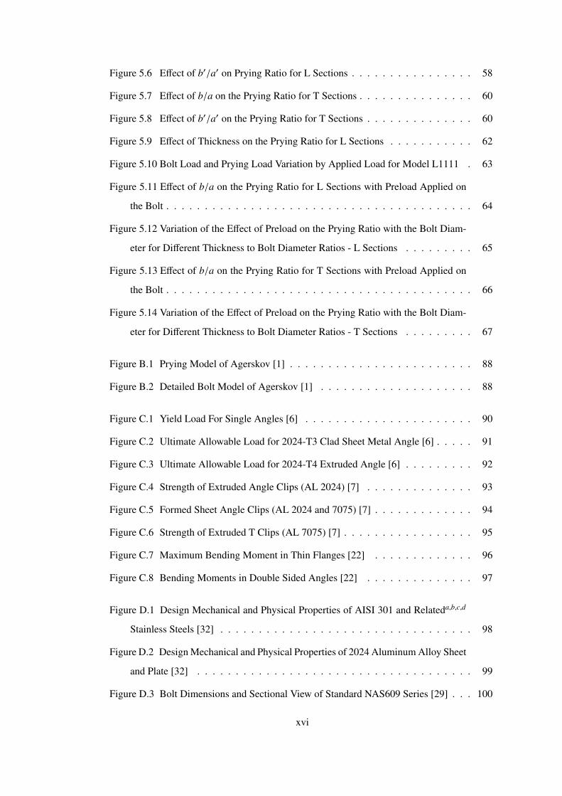
Figure 5.6 Effect of b′/a′ on Prying Ratio for L Sections . . . . . . . . . . . . . . . . 58

Figure 5.7 Effect of b/a on the Prying Ratio for T Sections . . . . . . . . . . . . . . . 60

Figure 5.8 Effect of b′/a′ on the Prying Ratio for T Sections . . . . . . . . . . . . . . 60

Figure 5.9 Effect of Thickness on the Prying Ratio for L Sections . . . . . . . . . . . 62

Figure 5.10 Bolt Load and Prying Load Variation by Applied Load for Model L1111 . 63

Figure 5.11 Effect of b/a on the Prying Ratio for L Sections with Preload Applied on

the Bolt . . . . . . . . . . . . . . . . . . . . . . . . . . . . . . . . . . . . . . . . 64

Figure 5.12 Variation of the Effect of Preload on the Prying Ratio with the Bolt Diam-

eter for Different Thickness to Bolt Diameter Ratios - L Sections . . . . . . . . . 65

Figure 5.13 Effect of b/a on the Prying Ratio for T Sections with Preload Applied on

the Bolt . . . . . . . . . . . . . . . . . . . . . . . . . . . . . . . . . . . . . . . . 66

Figure 5.14 Variation of the Effect of Preload on the Prying Ratio with the Bolt Diam-

eter for Different Thickness to Bolt Diameter Ratios - T Sections . . . . . . . . . 67

Figure B.1 Prying Model of Agerskov [1] . . . . . . . . . . . . . . . . . . . . . . . . 88

Figure B.2 Detailed Bolt Model of Agerskov [1] . . . . . . . . . . . . . . . . . . . . 88

Figure C.1 Yield Load For Single Angles [6] . . . . . . . . . . . . . . . . . . . . . . 90

Figure C.2 Ultimate Allowable Load for 2024-T3 Clad Sheet Metal Angle [6] . . . . . 91

Figure C.3 Ultimate Allowable Load for 2024-T4 Extruded Angle [6] . . . . . . . . . 92

Figure C.4 Strength of Extruded Angle Clips (AL 2024) [7] . . . . . . . . . . . . . . 93

Figure C.5 Formed Sheet Angle Clips (AL 2024 and 7075) [7] . . . . . . . . . . . . . 94

Figure C.6 Strength of Extruded T Clips (AL 7075) [7] . . . . . . . . . . . . . . . . . 95

Figure C.7 Maximum Bending Moment in Thin Flanges [22] . . . . . . . . . . . . . 96

Figure C.8 Bending Moments in Double Sided Angles [22] . . . . . . . . . . . . . . 97

Figure D.1 Design Mechanical and Physical Properties of AISI 301 and Relateda,b,c,d

Stainless Steels [32] . . . . . . . . . . . . . . . . . . . . . . . . . . . . . . . . . 98

Figure D.2 Design Mechanical and Physical Properties of 2024 Aluminum Alloy Sheet

and Plate [32] . . . . . . . . . . . . . . . . . . . . . . . . . . . . . . . . . . . . 99

Figure D.3 Bolt Dimensions and Sectional View of Standard NAS609 Series [29] . . . 100

xvi

Figure D.4 Bolt Dimensions of Standard NAS609 Series [29] . . . . . . . . . . . . . 100

Figure E.1 Code Generated for the Description of Models . . . . . . . . . . . . . . . 101

Figure F.1 Clip Flange Mesh Choices . . . . . . . . . . . . . . . . . . . . . . . . . . 114

Figure F.2 Bolt Mesh Choices . . . . . . . . . . . . . . . . . . . . . . . . . . . . . . 114

xvii

LIST OF ABBREVIATIONS

F Applied load per bolt

M Moment

B Total force on the bolt

B0 Preload applied to a bolt

Q Prying load

C Contact force between flange andbase plate at bolt location

β Bolt load ratio (B/F)

E Young’s modulus of elasticity

ν Poisson’s ratio

D Diameter of the bolt

a Edge distance of the bolt center

b Distance of the bolt center to theweb

w Pitch (depth of flange per bolt)

σ Normal stress component

τ Shear stress component

σy Yield stress

Acronyms

FEM Finite Element Method

FBD Free Body Diagram

xviii

CHAPTER 1

INTRODUCTION

1.1 Objective of The Thesis

Finite element method is a very important computational tool which is frequently used in

aircraft structural design and analysis, as well as in comparisons with analytical calculations.

Although very significant advancements have taken place in finite element methodology, in

many aeronautical applications simpler models are still being used in structural analysis of

aerospace structures. For instance, determination of internal forces is usually performed

by simpler finite element analysis employing simpler models. No doubt that this simplic-

ity mostly gives the quickest, thus time efficient results. On the other hand, some situations

like the prying effect in bolted connections that is the subject of this thesis, require more accu-

rate finite element models in order to extract meaningful results from a physical phenomenon.

The main expectation from such models is to represent the real system more closely. For in-

stance, prying load calculation requires contact description, which is essentially non-linearity

associated with boundary conditions. In such circumstances, correlation of the finite element

analysis with the results of analytical methods is also very crucial since the expectation from

higher fidelity models is to simulate the real structural behavior more closely.

Main goal of this thesis is to present a fundamental study on the determination of prying load

focusing on bolted connections in aircraft structures with classical analytical methods and

finite element solution. In the thesis, for the calculation of the prying load, several analyt-

ical approaches from civil engineering discipline are also reviewed. With the review of the

analytical approaches, it is intended to make a more clear explanation of the calculation and

effect of prying load. The current study does not only present the analytical approaches for

1

the calculation of the prying load, but also compares analytical solutions with the finite ele-

ment results to seek for if there exists a direct correlation between them or not. Comparisons

performed are used for checking the reliability of the finite element analyses and for selecting

suitable design tools to calculate the prying load and to study the prying effect in the bolted

connections.

1.2 Background

1.2.1 Aircraft Structures and Prying Effect

Aircraft structures are composed of many parts connecting with fasteners to each other. Most

of these fasteners are rivets, where there is not much tension load to be carried. On the other

hand, when tension loads are come up, bolts are being used. There are lots of bolt connection

types used on the airframe. This work mainly focused on the tension clip connections and

shear clip - stringer connections. Common trait of these connections is the requirement of

considering the prying effect.

Prying Load arises from the contact between the skin (or the base plate) and flange, as it

is illustrated at Figure 1.1 in the case external force pull upward away from the base plate.

Fasteners used at these type of connections are exposed to additional tensile load called Prying

Load. From Figure 1.1, it is clear that equilibrium of the L section necessitates the existence

of the prying load. Phenomenon caused by the prying load can be called as Prying Effect and

this subject is searched by many civil engineers [1, 2, 3, 4, 5] as well as aeronautical engineers

[6, 7].

In Figure 1.1, L section part may be considered as tension clip connecting two different parts

to each other. Due to tensile character of the connection, clip exerts prying effect. Tension

clip is exampled in the Figure 1.2.

2

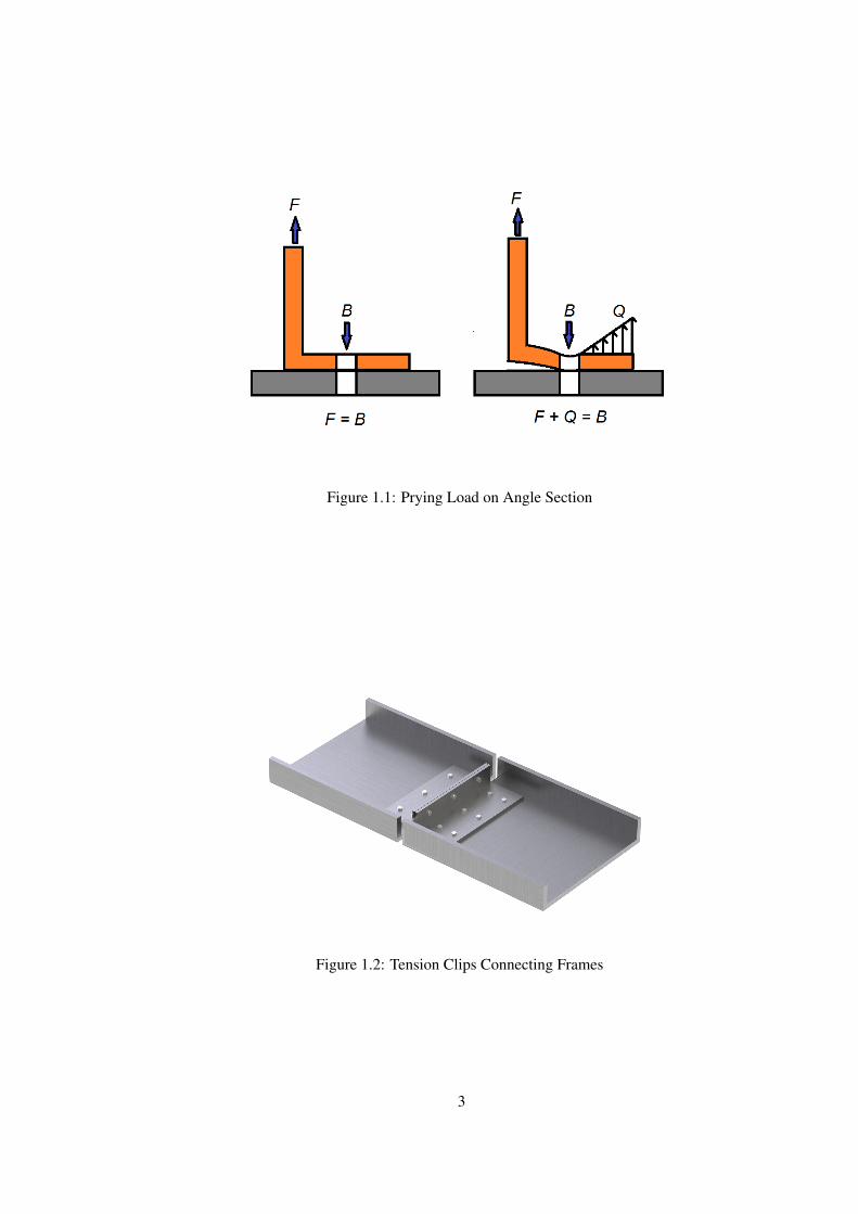
Figure 1.1: Prying Load on Angle Section

Figure 1.2: Tension Clips Connecting Frames

3

On the other hand, part with L section given in Figure 1.1 may also be considered as the

stringer section. External force F is applied on stringer section by shear clip. Shear clip

- stringer connections are mostly used at fuselage assembly in order to connect frame and

stringers as exemplified below in Figure 1.3 and these connections cause prying load to be

exposed on stringer flange.

Figure 1.3: Aircraft Fuselage Assembly and Shear-Clip Connections

Primary load paths like near regions the main landing gear require heavier connections. These

connections are assembled using fittings with thicker flanges. On the other hand, the light

tension clip connections carry relatively small tension loads and they are mostly used in three

different forms [6]:

1. Single Angles (L Section): This type of sections can be produced by extrusion or sheet

metal forming

2. Double Angles: Two single angles placed back-to-back

3. Extruded Tee Sections (T Section): These are mostly preferred for relatively high loads

In this thesis, forming effects of angle sections are not considered. Also behavior of double

angles are not included to the study. However, both L sections and T sections are examined.

Through out the thesis, it is decided to use clip term for L and T sections used in tensile

connections for simplicity. In this way, it is aimed to prevent mixed usage of clip and stringer

terms. One should be aware that all approaches are applicable on stringers as well.

4

1.2.2 Analysis of Connections Exposed to Prying Effect

Design and analysis of aircraft structures requires many cycles in order to achieve optimum

structural configurations. Throughout this heavy process, engineers need to solve problems

quickly without making concession on reliability. If the analysis process is examined, it is

seen that main tools are finite element based softwares such as Nastran, Abaqus etc. These

softwares are used frequently for global and local structural analyses. Most of the time, finite

element based structural analyses are planned as simple and fast as possible. For instance,

using contact between surfaces is not a very common application, since it is not as simple as

required.

Considering that high number of clip connections are used on aircraft assembly, it is almost

impossible to use finite element simulations with contact definition for all of the clip connec-

tions where prying effect exist. However, prying loads can be most accurately calculated by

incorporating contact definition, so there seems to be conflict between what is required and

what is feasible. Considering that in an aircraft assembly there are many clip connections, air-

craft structural analyses cannot be completed with finite element based tools and traditional

methods making use of analytical calculations becomes critical. Analyst need to create simple

models without contact definition and solve for the applied load on the clip which is expected

to be subjected to the prying effect. Obtained bolt forces of this analysis will not present the

correct bolt forces that is including the prying effect. After that, results of simulation and ge-

ometrical properties of the connection need to be merged and used with analytical methods.

In this way, correct bolt force can be calculated and analyst can decide whether the bolt and

the connection is safe or not.

In this study, primary analytical methods related with the prying effect, are examined and

shared briefly. Additionally, series of finite element analyses are performed for L and T

type clip connections by incorporating the appropriate contact definition for the purpose of

calculating the prying load. The analyses are performed within a large design space which

includes variation of bolt diameter, thickness of flange, bolt position and length of the flange as

the design parameters which are constrained by general design recommendations. Combining

the outcome of the analytical and finite element based prying load calculations, simple design

suggestions are made with regard to the prying effect.

5

1.3 Literature Review

Tension clip connections are very commonly used on aircraft assemblies. Similarly T-stub and

end plate beam-to-column connections are very common connections for civil engineering

applications. Although, they are used in different structures, all of these connections have

similar characteristics in terms of prying effect. Therefore, in the thesis investigation of prying

effect is not only restricted to aeronautical applications.

From aeronautical engineering point of view, prying effect is best presented by Bruhn and

Niu. Simplest approach presented here is from the work of Bruhn [6]. In order to show the

effect of the prying load, Bruhn considers the flange as a beam section and writes down one

of the classical static equilibrium equations which is the moment equilibrium about the toe of

the flange, as shown in Figure 1.4. Dimensions a and b shown in Figure 1.4 are used in the

moment equilibrium equation to calculate the prying load.

Figure 1.4: Prying Effect Representation from Bruhn [6]

Bruhn also provides an example plot of yield load data relating it with bolt spacing. It is

stated by Bruhn that reaching the maximum allowable strength of the connections is possible

only by using bolts in attachments. In case of rivet usage, steel ones might be the best choice.

Bruhn also emphasizes different design considerations. Acceptable and unacceptable designs

6

are summarized with the Figure 1.5. It is also added that, tension clip connections have mostly

bad fatigue characteristics. Therefore, using tension clip connections in cyclic loads should

be avoided.

Figure 1.5: Tension Clip Design Considerations of Bruhn[6]

Niu [7] also presents the main design concerns and experimental data curves to be used di-

rectly in the design phase. Niu discusses about the subject more clearly and widely compare to

the work of Bruhn. Differences between the formed sheet metal angles with extruded angles

due to material grain directions are presented on Figure 1.6.

Figure 1.6: Formed and Extruded Sections[7]

7

Niu also presents some important points that should be considered in the design of tension

clips. Some of these are listed below.

• Tension clips are used for comparably small loads (Tension fittings for primary loads)

• Tension fasteners need to be used

• Proper fillets or small bend radii need to be used for eccentrically loaded clips

• Clips are not suitable for repeating loads since there occurs high local stresses and large

deflections

• Clips should not be used in case of continuous load transfers as well

• Fastener installations are ranked in terms of their appropriateness (see Figure 1.7)

Figure 1.7: Fastener Installation for Clip Connections [7]

Niu also has allowable load plots for formed sheets made of 2024 and 7075 alloys, for angles

and tee sections (See Appendix C). In addition to the plots given, static equilibrium equation

for the fastener tension load is also provided by Niu likewise Bruhn. Although Bruhn assumed

that prying force acts at the tip of the flange Niu uses k constant for placing the prying force

which is concentration force representation of the contact force distribution between flange

and base structure as shown in Figure 1.8. Besides, Niu comments that calculation of k is

impossible since parameters like geometry and material of the clip; material, type and location

of the fastener; preload applied on fastener; shape of prying load curve all affect the value of

k.

8

Figure 1.8: Prying Load Distribution by Niu[7]

While aircraft engineers try to simplify the analysis of bolted connections as much as possible,

civil engineering approach is to get close results by using formulas generated through many

experiments. Additionally, reader is warned about the differences between the two disciplines

in terms of materials used, magnitude of the loads carried,and geometrical dimensions of the

structures (i.e. thickness of flange, diameter of bolt etc.).

In terms of the bolted connection and prying load issues, civil engineering database is quite

rich compared to all others. This is why the most of the sources presented in this thesis

are based on researches of civil engineers. Many researchers (Douty and McGuire, 1965;

Kato and McGuire, 1973; Nair et al., 1969; Agerskov, 1979; and Kennedy et al., 1981) have

developed various methods on prying effect on bolted connections. Some of these works are

introduced here briefly.

Douty and McGuire [3] performed experiments on variety of T-stub and end-plate moment

connections. According to the results of these experiments ultimate resisting moment of

flange, tensile load tractions of bolts with increasing applied load, slip conditions of bolts

and the prying force for varying geometrical and loading conditions are investigated. Authors

emphasize that calculation of prying forces with completely analytical methods is impossi-

ble. First of all, an approximate theory is generated based on three deformation equations of

local expansion of plate at bolt line, elongation of bolt and deflection of middle surface of the

flange. This approximate approach is divided into two main parts which are basically before

bolt line separation and after bolt line separation conditions. Main difference between these

conditions is the contact between the flange and base plate. Finally, these prying formula-

9

tions are supported with empirical parameters and tuned. Computed and observed results are

compared. Study ends with the authors design suggestions.

Nair et al. [5] conducted series of tests on T-stubs in order to classify the behavior ASTM

A325 and A490 bolts under prying load. These tests were mainly static tests in which the

load is increased till the failure, and dynamic tests which expand the study to fatigue char-

acteristics. Data obtained from the static tests are evaluated and presented as calculations of

prying forces depending on the geometry (i.e. flange thickness) of the connection and the

applied force.

Kato and McGuire [8] present the comparisons of the results of an analytical approach derived

and experiments performed. Study mainly focus on relationship between bolt and flange

strengths while considering post-elastic conditions such as strain hardening. Axial loading

conditions on bolts are examined depending on the varying conditions of preload, stiffness of

the bolt and stiffness of the flange. Comparisons between experiments and theoretical calcula-

tions shows 30 percent error at most. Study focuses on bolt efficiency where it may be defined

as the ability of using all capacity of the bolt directly for the connection purposes. In other

words, bolt efficiency may be described as the ability of avoiding the bolt to carry unwanted

loads like prying load, in addition to the main loading. It’s emphasized that bolt efficiency

does not depend on the ratio of flange thickness and bolt diameter, but also depends on all

other flange and bolt dimensions such as bolt head diameter, width of flange etc. However, it

is mentioned that connections with heavier flanges present relatively higher bolt efficiencies

since there exist less prying forces.

Agerskov [1] basically established experiments in order to measure prying forces for different

geometries, loading conditions, etc. Additionally, study contains the analytical approach and

derivation of general formulation. This formulation adds the effect of the shear stresses in the

section of the flange which is not taken into account in many other studies. Agerskov, collects

experimental results in two groups. One group is the case when the separation of flange at bolt

line occurs before reduced yield moment is reached in T-stub flange. Reduced yield moment

is described as moment that corresponds to full plastification of the section. The other group

is the case when the separation occurs after reduced yield moment is reached. Both thick

and thin flange plates are covered by the experimental results of Agerskov. All collected

results are compared with already existing analytical studies of Douty and McGuire [3] and

10

the method given by AISC [9] which is originally work of Thornton [10] and Swanson [11].

Comparison study presents a good agreement between all results where AISC results are most

conservative them all.

Fisher et al. present the analysis and design considerations for tension type connections at

17th chapter of book entitled ”Guide to Design Criteria for Bolted and Riveted Joints” [2]. In

terms of analysis and prediction of prying force, authors summarize the existing models like

Douty and McGuire [3], Nair [12] and Agerskov [1]. Since those models are applicable only

for specified conditions and not applicable for various bolt and plate combinations, authors

give more general methodology based on the work of Struik and de Back [13]. After sum-

marizing all these methods, related design recommendations including the static and fatigue

behavior of T-Stub connections and bolts are presented.

Krishnamurthy’s study [14] includes finite element modeling of several models. Due to diffi-

culties in computing of 3D models of those times author tried to create correlations between

several 2D models and very simplified 3D models. At the end, he concluded that there was

no significant prying effect in the configurations that were studied.

Kennedy et al. [15] explained the behavior of tensile type connections by considering the

loading in three main parts. First of these parts is called as thick plate behavior since it

describes the condition of no prying forces. For this part, it may be easily said that bolt forces

are directly correlated with the applied force. On the other hand, third part is called as thin

plate behavior where the prying forces are quite effective. Here, as it is expected, bolt forces

are sum of applied forces and prying forces. Finally the second part is the one that forms

the transition between part one and three, so called intermediate plate behavior. Kennedy

presented equations to predict prying forces for each type of behavior.

Swanson [11], compared several analytical prying models which are methods of Struik and

de Back [13], Nair et al. [12], Douty and McGuire [3], Kato and McGuire [8], and Jaspart

[16]. Among all models, Struik and de Back’s model is found to present least difference with

respect test results.

In addition to analytical models, many researchers like Kukreti et al. [17], Krishnamurthy

and Thambiratnam [4], Chasten and Driscoll [18], Maggi et al. [19] and Kamuro et al. [20]

performed comparative finite element analysis in order to investigate prying effect.

11

1.4 Structure of The Thesis

In analytical part of the thesis, basic calculations and statical equilibrium equations are shown

for the flange which is considered as a beam. These calculations are required so that one

can understand the behavior of the connection better. After the introduction of the basic

calculations, some of the more complex formulations performed by other researchers are

shared briefly. By presenting more complex approaches, it is aimed to understand then physics

of the prying effect better.

Numerical simulation models are performed in the Abaqus software environment in order to

obtain benefits of simple modeling process and automation ability. Details of this process

like element types, boundary conditions, contact definition and materials are all described in

Chapter 3. In this chapter, parametric modeling performed and algorithm generated for the

automatized process are also described briefly. Appendix A gives the script generated for the

parametric modeling performed in Abaqus.

In Chapter 4, in order to check the reliability of the numerical models prepared with Abaqus

software, prying loads determined by the finite element are compared with the experimental

and theoretical results presented by Agerskov.

Ability of performing sequential analysis gained from the algorithm generated, gives the op-

portunity of searching how geometrical dimensions involved in the bolted connections effect

the prying load. In addition to geometrical affects on prying ratio, affect of bolt preload is also

investigated. Results of the parametric study on prying load are presented in the Chapter 5.

In this chapter, prying load results are tried to be organized in such a way that, a designer or

an analyst makes use of the outcome of the parametric study in designing bolted connections.

In the conclusion chapter, performed study is summarized briefly and benefits of the cur-

rent study are presented. At the end of the thesis, one may find additional informations in

Appendix part like sample Phyton script, properties of test specimens of Agerskov, referred

tables and figures and complete table of results obtained from the series of analysis performed

in Chapter 5.

12

CHAPTER 2

ANALYTICAL STUDY

2.1 Behavior of the Tension Clip Connections

The behavior of the tension clip connections can be best understood by drawing their free

body diagrams. Angle sections deflect as it is shown in the Figure 2.1 where Q denotes the

resultant prying force. Assuming small deformations, we may consider that external force

F can be assumed to be acting in the direction 1 vertically upwards. It is also assumed that

flange material is relatively soft compared to the bolt material.

Figure 2.1: Free Body Diagram of the Angle Section

13

For general prying force distribution, concentrated point force acting at the centroid of the

distributed prying load can be placed at k.a distance from the bolt center (where 0 ≤ k ≤ 1).

However, many researchers accept prying load as a line load acting at the edge of the flange,

such that k = 1. For general k value, taking moments about section 2 yields

QF

=bka

(2.1)

As it is seen from Equation 2.1, with the assumption of k = 1 the ratio of the prying force

to the externally applied force becomes b/a. On the other hand, assuming triangular prying

force distribution k = 2/3 yields

QF

=3b2a

(2.2)

It can thus be concluded that if the centroid of the distributed prying load is closer to the

bolt, the resulting prying force is higher compared to assuming that prying force is a line load

acting at the edge of the flange.

When T sections are examined, symmetry plane is defined in the middle of the section, as

shown in Figure 2.2. One can easily see that it is hard to obtain Q/F through overall force

and moment equilibrium equations since the system of static equilibrium has undetermined

boundary conditions.

It is noted that instead of writing equilibrium equations on overall section, the T section can

be divided into subsections as it is illustrated in Figure 2.3.

14

Figure 2.2: T Section Overall Free Body Diagram

Figure 2.3: T Section Free Body Diagrams

15

Second subsection gives the equilibrium for the calculation of sectional bending moment:

M =Fb2

(2.3)

On the third subsection which includes the part from bolt to the tip of the flange, moment

equilibrium can be written around section 2 for an arbitrary k value. Equation 2.4 gives the

resultant equation. In the derivation of Equation 2.4, F acting on the flange is assumed to be

close to the bolt center line.

Qka = M (2.4)

and the corresponding Q/F ratio is

QF

=b

2ka(2.5)

In condition of k = 1, ratio of the prying force Q to the external force F yields b/2a. On the

other hand, for the triangular prying load distribution, the ratio becomes

QF

=3b4a

(2.6)

From basic statics, the ratio prying load to the applied external load can be determined as

described above. However, it should be noted that the use of equilibrium equations is a sim-

plified approach for the calculation of prying forces and the resulting bolt forces. Since the

main objective in determining the prying forces is the determination of actual bolt forces in-

creased by prying forces, it is better to discuss about the bolt connections and their behavior

under tensile loading.

Single bolt connecting two plates directly carries the load which is equal to the external load

in the case of no pretension is applied on the bolt. On the other hand, if there is pre-tension B0

on the bolt, bolt carries this load initially when there is no external force. Bolt force increase

with increasing applied load, but this increase is slower than the increase of applied load so

that they coincide at the separation of plates as it is shown in Figure 2.4.

16

Figure 2.4: Bolt Force Variation Due to Applied External Load on Preloaded Bolt [2]

Increase of the bolt force depends on the stiffness of the connection. In the case of heavy

flanges, the bolt force line is flatter, whereas it is steeper for lighter flanges. Apart from the

stiffness of the connection, variation of bolt force depends on the type of the connection.

Existence of prying effect creates an offset on bolt force as shown in Figure 2.5. It is noted

that as the external force is increased, there comes a moment where the separation of the

plates occur. At this point, prying force reduces to zero. In Figure 2.5, it is seen that prying

force reduces as the external force is increased further indicating that complete separation of

the plates is about to occur.

Another definition of the prying effect is presented in ESDU document 85021 [21]. Figure

2.6 shows the variation of loads in components with respect to applied external load F. Bolt

load B curve presented by initial slope γb which is related with the connection stiffness. γb

slope becomes flatter as the flange stiffness increases. Since base plate is assumed rigid in

this thesis, γb becomes horizontal. In addition to bolt load , Figure 2.6 also shows contact

force variation between plates. Initial contact force C is formed due to bolt preload Bo. While

F is increased and separation of flange around bolt region occurs, contact force C decreases

whereas the prying force Q is formed and increases. Document also emphasize that applica-

tion of pretension on the bolt delays the separation of the bolt.

17

Figure 2.5: Effect of Prying on Bolt Force Variation [2]

Figure 2.6: Actual Effect of Prying on Bolt Force Variation [21]

18

2.2 Prying Load Calculation Approaches of Bruhn and Niu

Bruhn presents a simple analytical approach by using static equilibrium equations on the free

body diagram shown in Figure 1.4. By using equilibrium equations, prying load ratio can be

calculated as [6]

QF

=ba

(2.7)

On the other hand, Niu emphasizes the impossibility of exact calculation of prying effect due

to plenty of dependencies like [7]:

• Geometry and material of the clip

• Type, material and location of the fastener

• Preload in fastener

• Distribution shape of contact forces forming the prying load

• Thickness ratio of flange and web

At this point, it should be pointed out that strength of tension clip connection depends both on

bolt and clip strength. Failure of clip mostly occurs due to internal bending moments either

at the corner of the web and flange (this is why fillet radius is recommended) or at the flange

location where the tip of washer or bolt head pushes down, as shown in Figure 2.7.

Figure 2.7: Bending moments acting on flange[22]

19

Niu points the requirement of conducting series of experiments in order to obtain reliable

design data, similar to the practice followed by the aircraft manufacturers. Some of these data

provided by Bruhn and Niu are given in Appendix C. ESDU document 84039 is also available

in Appendix C. Data provided by these curves are useful tools for the estimation of ultimate

strength of clips.

Besides clip strength, bolt strength is also important for the estimation of limitations of the

connection. Although, Niu and Bruhn provide sample curves considering the bolt limitations,

these curves are not applicable for the various type of connections (See Figure C.1 and C.4).

Due to this reason, this study mainly focuses on actual bolt forces increased by prying effect

and tries to produce useful data and knowledge in order to fill this gap.

2.3 Douty and McGuire’s Method

Douty and McGuire emphasize that analytical methods cannot determine prying load directly

without empirical modifications. Their work presents a useful analytical approach which is

supported by experiments. Before the application of external load, only pretension load B0

exerts on the T-stub flange as it is illustrated in Figure 2.8a.

Figure 2.8: Simplified Prying Model of Douty and McGuire [3]

After external load is applied, force on the bolt becomes (F + Q + C) where C stands for the

compressive contact force between flange and base plate and where Q stands for prying force

acting at the tip line of the flange, as shown in Figure 2.8b.δ describes the deflection of the

middle plate of flange. Although δ has positive values after external load is applied, bolt line

20

of the flange is considered to be in contact with the base plate until a threshold external load

is applied. This is explained with the dishing effect on the upper surface of the flange due to

preload B0. As a result of this dishing effect, bolt region is compressed and thickness of this

region is smaller. It is said that the bolt region of the flange will not separate until the flange

thickness is restored at this region as it is shown in Figure 2.8b. Restoring the thickness of

flange will be seen as the expansion of the flange at lower surface. Before the separation,

downward expansion of the flange plate at the bolt location is given by

δ =(B0 −C)lp

ApEp=

(B0 −C)rp

(2.8)

where lp is effective thickness of flange, Ap is effective compressed area and Ep is the effective

stress-strain ratio which are all collected under the term rp. Similarly, bolt elongation is given

by

δ =(B − B0)lb

AbEb=

(B − B0)rb

(2.9)

All forces are assumed to be uniformly distributed through flange width, w and from simple

moment area principles, deflection of middle plate of flange at bolt location is determined as

δ =ab2

E( wt312 )

{F2−

aB

[13

(ab

) + 1]}

Q (2.10)

Solving equations given above for Q results with the following relation.

QF

=

12 −

(Ewt3)(12ab2)(rb+rp)

ab ( a

3b + 1) +(Ewt3)

(12ab2)(rb+rp)

(2.11)

Equation 2.11 is valid until flange separation at bolt location occurs. After that point, contact

load between plates vanishes out, C becomes 0 and Equation 2.11 becomes

QF

=

12 −

(Ewt3)(12ab2rb) (1 −

B0F )

ab ( a

3b + 1) +(Ewt3)

12ab2rb

(2.12)

21

Douty and McGuire’s approach depends on the assumption that prying force acts at the tip of

the flange. This assumption is reasonable for a limited length a which is the distance from the

bolt to the edge of the flange. Authors point out that the large values of a are questionable.

Furthermore, at design suggestion part of the study it is assumed that a = 1.25b when the case

is actually a ≥ 1.25b.

Both of equations 2.11 and 2.12 are generated assuming that the flange remains in elastic

range. Complexity of these equations forced researchers to simplify them. First simplification

step results with the Equation 2.13 which is quite similar to the Equation 2.12 [2, 3, 11].

QF

=

12 −

(wt4)(30ab2Ab)

ab ( a

3b + 1) +(wt4)

6ab2Ab

(2.13)

However, Equation 2.13 was not found to be practical in terms of design purposes and further

simplifications are performed [2, 11, 23]. As a result, only most dominant factors of the

prying effect retained and equation 2.14 is obtained.

QF

=

(3b8a−

t3

20

)(2.14)

2.4 Agerskov’s Method

Agerskov’s study [1] resembles to the Douty and McGuire’s in terms of road map of the work

done. Agerskov also presents an approach starting from static equilibrium conditions to the

prediction of prying forces. In addition to the previous studies, Agerskov adds the effect of

shear in flange which is considered to be a conservative approach[2, 23].

Agerskov divides study into two cases due to the sequence of occurrence of flange separation

at bolt region or reaching yield moment at the inner end of the flange as illustrated in Figure

2.9.

22

Figure 2.9: Prying Model of Agerskov [1]

Agerskov starts with the case where flange separation occurs before yield moment is reached.

Agerskov reorganizes the method suggested by Douty and McGuire [3, 24] so that inelastic

effects are included as a limitation. In addition to inelastic effects, Agerskov takes the effect

of shear in flange section into account as τ = F/(wt). Shear value is placed in von mises yield

criterion σy =√σ2 + 3τ2. As a result, allowable normal stress at the flange section reduces

to σ =

√σ2

y − 3τ2 and plastic moment at inner end of the flange becomes

M2,y =

14

wt2

√σ2

y − 3( Fwt

)2 (2.15)

where moments at section 1 and 2 are M1 = Qa and M2 = F(a + b) − Ba, respectively.

Equating M2 to M2,y gives

F(a + b) − Ba =

14

wt2

√σ2

y − 3( Fwt

)2 (2.16)

23

Similar to Douty and McGuire’s work (See Equations 2.8 to 2.10), Agerskov also considers

plate deflection at the middle surface of the flange at the bolt location (δp) and the bolt elon-

gation (δb) in the formulations. Considering that the flange length is given by l = 2(a + b),

and non-dimensional length α is given by a/l, Agerskov presents δp as

δp =l3

Ewt3

[F

(32α − 2α3

)− B

(6α2 − 8α3

)](2.17)

On the other hand, bolt elongation is given below as the summation of elongation at flange

separation condition and elongation after flange separation due to increase in the bolt force

(∆B = B − Bsep).

δb =110

B0tEAs

+B − Bsep

EAsk (2.18)

where As the area of the bolt and k = 0.50ls + 0.72lt + 0.46ln + 0.20lw which depends on the

dimensions shown in Figure 2.10.

Figure 2.10: Detailed Bolt Model of Agerskov [1]

Finally, Equation 2.19 is obtained by equating the total elongation of the bolt and deflection

of the flange at the bolt location δb = δp.

110

B0tAs

+B − Bsep

Ask =

l3

wt3

[F

(32α − 2α3

)− B

(6α2 − 8α3

)](2.19)

24

After obtaining equations 2.16 and 2.19, they need to be solved for F and B simultaneously.

Results will give prying force as Q = B − F since this is the case which assumes flange yield

moment stress is reached after flange separation at bolt location occurs. In other words, when

yield moment stress is reached, there is no contact force between flange and base plate at bolt

location.

Similarly, case which flange separation at bolt location occurs after the yield moment stress

is achieved, can be solved. There is only one difference between this case with the previous

one. The contact force C between the plates at bolt location will be still available when yield

moment stress is reached in the flange. Under these circumstances, static equilibrium gives

prying force as Q = (B − C) − F and Q can be calculated after simultaneous solution of

equations given below.

Contact force between plates at bolt location is presented as given by Equation 2.20.

C = B0Bsep − BBsep − B0

(2.20)

Equation 2.16 is reorganized as Equation 2.21 since contact force C is taken into account.

F(a + b) − (B −C)a =

14

wt2

√σ2

y − 3( Fwt

)2 (2.21)

Similarly Equation 2.19 is modified such that it takes contact force C into account. Besides,

(B − Bsep)k/As term is vanished out because the bolt force B is assumed to be less then Bsep

since the flange at bolt location is not separated.

110

B0 −CAs

t =l3

wt3

[F

(32α − 2α3

)− (B −C)

(6α2 − 8α3

)](2.22)

25

2.5 Struik and de Back’s Method

Struik and de Back also concentrate on the sectional forces, moments and equilibrium equa-

tions of the flange to determine the prying force. Classical prying model is drawn with the

dimensions shown in Figure 2.11.

Figure 2.11: Prying Model of Struik and de Back [2]

In Figure 2.11, α is the ratio of moment at the bolt location (section 1) to the flange moment at

the web face (section 2). δ is the ratio of the sectional area at the bolt location to the sectional

area of the flange at the inner end (section 2). According to Swanson [11] δ = 1−D/w where

D is the diameter of the bolt and w is the flange length per bolt. Related equilibrium equations

are presented in Equations 2.23a to 2.23d [2].

M − Fb + Qa = 0 (2.23a)

F + Q − B = 0 (2.23b)

Qa − δαM = 0 (2.23c)

M =14

wt2σy (2.23d)

It should be pointed that Equation 2.23d represents the plastic moment capacity of the flange.

It was also given in a different form in Equation 2.15. Solving these equations gives the

critical values of bolt force and the corresponding minimum flange thickness.

26

B =

[1 +

δα

(1 + δα)ba

]F (2.24)

t =

{4Bab

wσy [a + δα(a + b)]

}1/2

(2.25)

Prying force ratio for this critical condition can then be written as

QF

=

[δα

(1 + δα)ba

](2.26)

Apart from this approach, Struik and de Back improve the results by modifying the a and b

values as shown in Figure 2.12. This modification does not change the equations but only

replaces the values of a and b with a′ and b′.

Figure 2.12: Struik Model with Bolt Head Force and Internal Moment Distribution on Flange[11]

27

There has been various discussions on the expressions for a′ and b′ [25]. One can easily figure

out that heavier flanges present less offset between the position of average bolt head load and

the actual bolt line due to less flange deformation. On the other hand, in light flanges offset

is higher. Among the suggestions for the expressions for a′ and b′, most powerful and simple

one is a′ = a + D/2 and b′ = b − D/2 proposed by Fisher and Struik [2].

Fisher and Struik [2] also emphasize that the assumption of prying load as a line load acting

at the tip of the flange is valid only under the condition of a ≤ 1.25b.

Struik’s model is also modified by Thornton [10] which is also the suggested method by AISC

[9]. Equation 2.23d is modified in order to reduce the critical moment such that the solution

is more conservative. Modified version of the equation is given by Equation 2.26.

M =18

wt2σy (2.27)

2.6 Design Considerations in terms of Prying Effect

Considering all studies presented, it might be possible to suggest some additional design

approaches for aircraft design and analysis procedures. Civil engineering applications con-

sider larger size structures, and corresponding analytical studies depend on Imperial units.

When these analytical methods are used for aircraft applications, dimensions are small (i.e.

thickness), and higher order terms become insignificant. For example, simplified version of

Douty’s formula is one of the most applicable prying force ratio. In Douty’s formula given

by Equation 2.14, since t3 << 20 higher order term t3 can be neglected, and Equation 2.14

becomes

QF

=

(3b8a

)(2.28)

28

Agerskov’s method is iterative and calculations are more complicated compare to the others.

Due to this fact, it is not suggested as possible design tool. However, Struik’s prying formula

is also very similar to the one simplified Douty’s equation. Equation 2.25 can be written as

QF

=

(3b′

7a′

)(2.29)

Equation 2.29 is obtained by assuming α = 1 which is quite reasonable for constant cross

section. Besides, Equation 2.29 is valid only when the fastener pitch is equal to four times the

diameter of the fastener (w = 4D). Thus, δ becomes 3/4 [11], and Equation 2.29 is obtained.

One should be aware Equations 2.28 and 2.29 are valid for T sections. This approach might

be also used for angle sections if the ratio between T section and L section is assumed two.

Then, for L sections, formula given by Douty and McGuire becomes

QF

=

(3b4a

)(2.30)

Douty’s formula and Struik’s formula for T sections are almost same. Although these ap-

proaches give very rough results, it is possible to use them as a pre-design tool. If these

approaches will be used for aircraft design, they also need to meet the requirements of avia-

tion. First of all, Fisher and Struik suggest a to be less than 1.25b. On the other hand, general

aircraft design knowledge says that edge distance of the bolt should be greater than two times

the fastener diameter [6]. If these limitations are combined, a bound on a can be obtained as

2D ≤ a ≤ 1.25b (2.31)

29

From Equation 2.31 it is concluded that b needs to be greater than 1.6D. Additionally, Tim-

oshenko [26] states that we f f = 2b + Dhead. If one ignores the bolt head diameter, we f f is

approximately equal to 2b as shown in Figure 2.13. If effective flange length for bending can

be assumed to be equal or less than the fastener spacing (we f f ≤ w = 4D), then 2b ≤ 4D [9].

Combining both constraints on b gives

1.6D ≤ b ≤ 2D (2.32)

Figure 2.13: Effective Flange Length for Bending [9]

Limitations presented above are needed to be considered as the definition of design space

used in this thesis. These limitations are required for

• Having finite number of situations to investigate

• Keeping all geometrical decisions acceptable according to general aircraft design knowl-

edge

• Ability to compare obtained results with the results obtained from the methods in liter-

ature

Usage of these limitations are explained in Chapter 5. In Table 5.1, one can see that b values

are within the limitations although a values are not, since it is decided to check the validity of

a ≤ 1.25b which is suggested by Fisher and Struik [2].

30

CHAPTER 3

FINITE ELEMENT MODELING

In this thesis, prying loads are examined in tensile connections. Aircraft manufacturers mostly

prefer to conduct series of experiments for various cases in order to obtain actual prying loads.

Design curves are created from collected data of experiments. In this thesis, prying loads

are obtained from series finite element analyses instead of experiments, so that comparable

results are obtained. Since prying load itself is a contact force between plates, finite elements

analysis need to include contact definition. In this chapter, details of finite element modeling

is presented.

3.1 Mesh Description

All of the angle and tee section clip models are created by using linear 8 node-hexagonal-brick

element of Abaqus, C3D8. Through flange thickness there are at least four lines of elements in

order to calculate and visualize the stress distribution better. Medial axes meshing technique

is [27] used since it reduces the face partition requirements where there is a curved region like

a fillet, round or a hole. Benefits of medial axes meshing technique is presented in Appendix

F. Only one partitioning is used on the upper face of the flange, where the washer region

is defined for the contact definition. Figure 3.1 shows the three dimensional finite element

model of the clip.

Bolts are again modeled by C3D8, 8 node-hexagonal-brick elements. Although the bolt ge-

ometry is obtained by revolution of surface, elements are created again using the medial axes

meshing technique. As a result, creation of 6-node-wedge elements at the center line of the

bolt is prevented as it is seen in Figure 3.2.

31

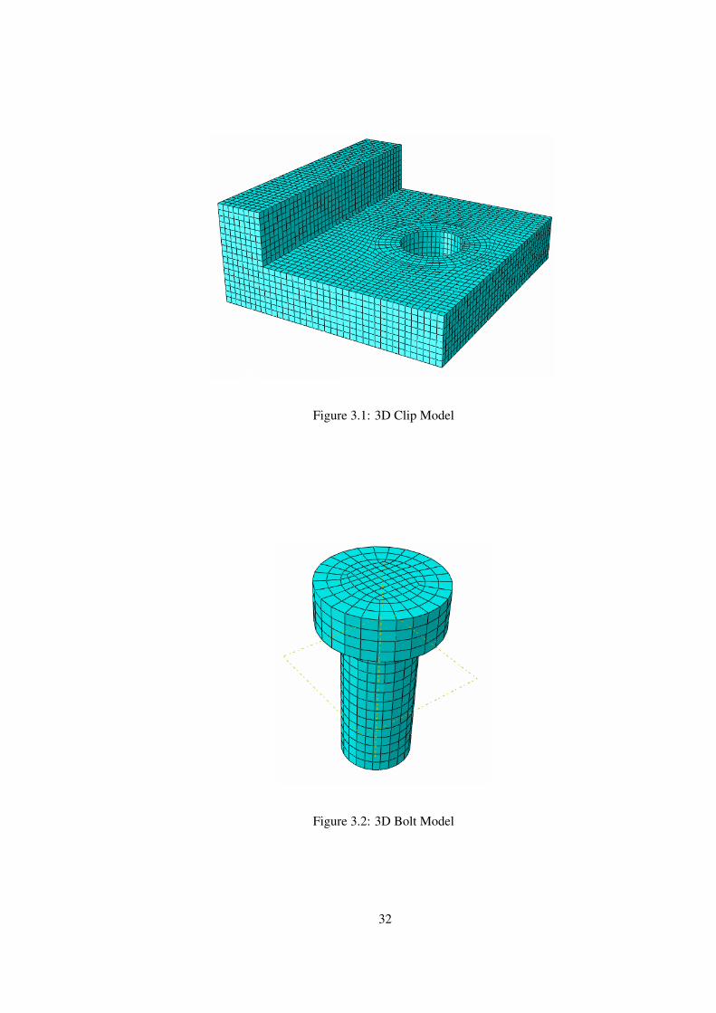
Figure 3.1: 3D Clip Model

Figure 3.2: 3D Bolt Model

32

Base plate is assumed rigid like many other studies [3, 1, 4]. Rigid plate is placed under

the clip. This simple plate is modeled without any elements, instead, it is geometrically

constrained with respect to one of its corner points and fixed in the space. In Figure 3.3,

whole finite element model including the rigid plate can be seen.

Figure 3.3: Complete View of 3D Model of Bolted Clip Connection

3.2 Boundary Conditions and Loads

It should be noted that in the present study, it is assumed that the bolt-clip combination that

is modeled is repeated in the depth direction. Therefore, modeling an angle or a tee-section

clip connection requires slightly different set of boundary conditions. Both of them require

suitable boundary conditions to account for the repetition of the sections comprising bolt-clip

combination. This way, only one bolt region is modeled. Behavior of these same depth repeat-

ing sections are assumed to be exactly same, since the load is also assumed to be uniformly

distributed. As a result, it is concluded that the regions between these sections will remain

plane as illustrated in Figure 3.4. The boundary conditions shown in Figure 3.4 imply that side

faces of the L shaped clip remain XY plane since it is constrained on Z axis (demonstrated as

33

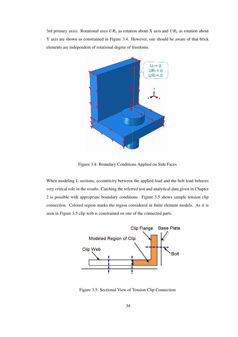
3rd primary axis). Rotational axes UR1 as rotation about X axis and UR2 as rotation about

Y axis are shown as constrained in Figure 3.4. However, one should be aware of that brick

elements are independent of rotational degree of freedoms.

Figure 3.4: Boundary Conditions Applied on Side Faces

When modeling L sections, eccentricity between the applied load and the bolt load behaves

very critical role in the results. Catching the referred test and analytical data given in Chapter

2 is possible with appropriate boundary conditions. Figure 3.5 shows sample tension clip

connection. Colored region marks the region considered in finite element models. As it is

seen in Figure 3.5 clip web is constrained on one of the connected parts.

Figure 3.5: Sectional View of Tension Clip Connection

34

Left end of the colored region in Figure 3.5, is the upper surface of clip web. In order to

simulate the bolt connection close to the upper surface, it is constrained about X axis as

shown in Figure 3.6.

Figure 3.6: Boundary Condition Applied on Top Surface

On the other hand, when T sections are handled, one can easily see that free body diagram

of this section will not present an eccentricity between loads. Besides, there will not be any

lateral motion behavior on the top surface of the clip web. However, T section modeling has

different requirements like symmetry plane definition. In the present study, instead of mod-

eling both of two flanges of the clip section, symmetrical half is used. By using half model

computation time is reduced, and modeling is considered to be an easier due to the similarity

with the L shaped model. This similarity makes it possible to make changes in parametric

modeling by small manipulations of the script file of the L section which is discussed in the

parametric modeling section of this chapter. Thus, T section models are generated without

complete re-modeling. Halving the T sections should not be problem as long as the analyst

applies corrected external load on the model. Instead of applying total load of the related

connection, analyst needs to apply external load per single bolt. Figure 3.7 shows the sym-

metry boundary condition applied on the half model of the T section. On the back face of the

clip web, out-of-plane rotations and deflections are fixed to provide the necessary symmetry

boundary conditions. Again, it should be emphasized that rotational degree of freedoms are

inapplicable on brick elements.

35

Figure 3.7: Symmetry Boundary Condition Applied on Back Surface of the Clip Web

In addition to clip, there is another boundary condition defined on the bolt. Bolt is simply

fixed from its grip surface. Figure 3.8 shows the corresponding boundary condition on the

bolt.

Figure 3.8: Boundary Condition Applied on the Bolt

36

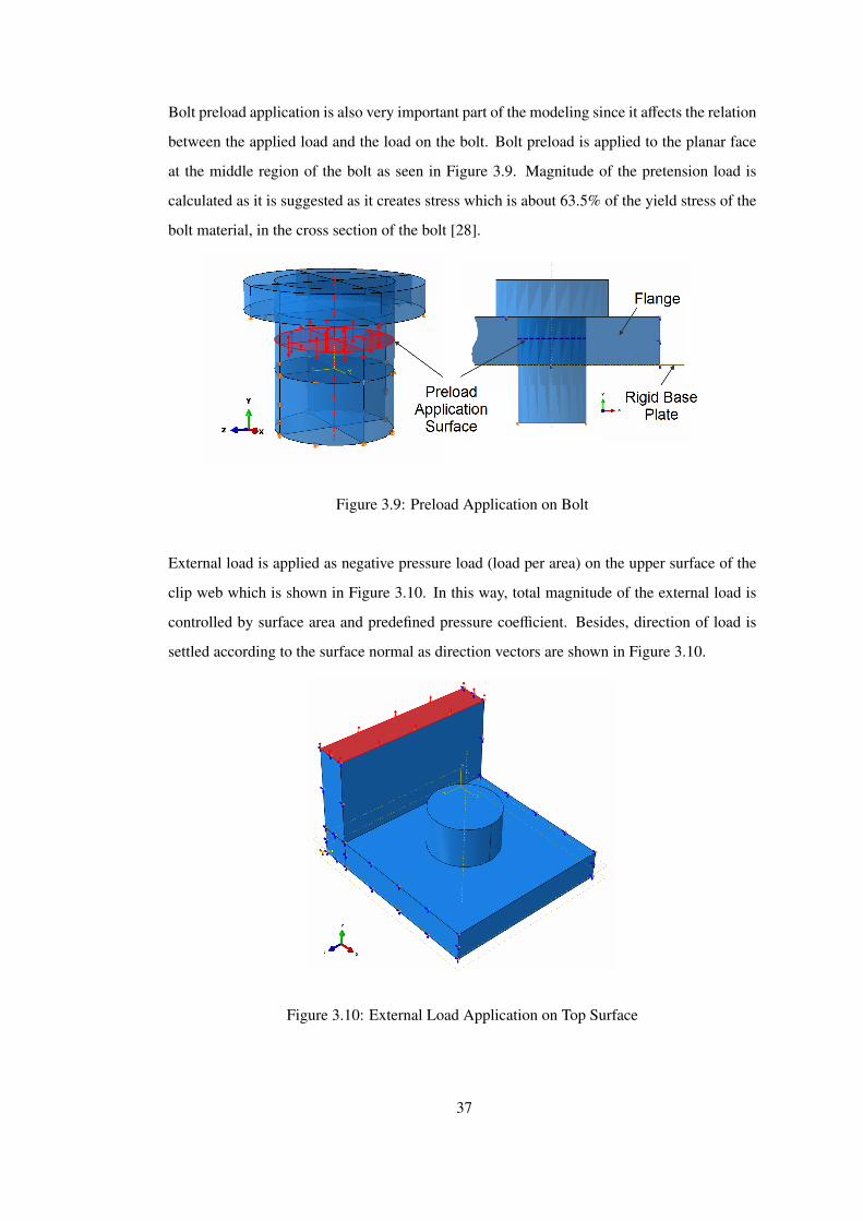
Bolt preload application is also very important part of the modeling since it affects the relation

between the applied load and the load on the bolt. Bolt preload is applied to the planar face

at the middle region of the bolt as seen in Figure 3.9. Magnitude of the pretension load is

calculated as it is suggested as it creates stress which is about 63.5% of the yield stress of the

bolt material, in the cross section of the bolt [28].

Figure 3.9: Preload Application on Bolt

External load is applied as negative pressure load (load per area) on the upper surface of the

clip web which is shown in Figure 3.10. In this way, total magnitude of the external load is

controlled by surface area and predefined pressure coefficient. Besides, direction of load is

settled according to the surface normal as direction vectors are shown in Figure 3.10.

Figure 3.10: External Load Application on Top Surface

37

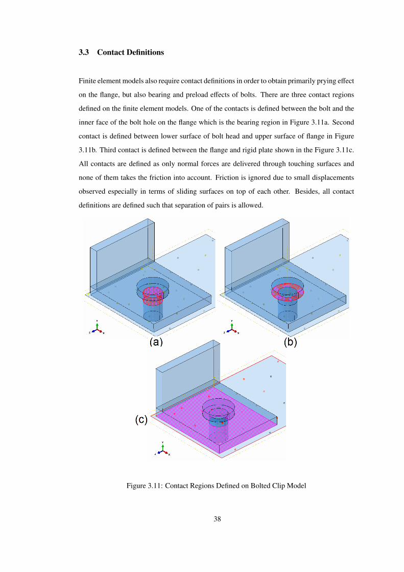
3.3 Contact Definitions

Finite element models also require contact definitions in order to obtain primarily prying effect

on the flange, but also bearing and preload effects of bolts. There are three contact regions

defined on the finite element models. One of the contacts is defined between the bolt and the

inner face of the bolt hole on the flange which is the bearing region in Figure 3.11a. Second

contact is defined between lower surface of bolt head and upper surface of flange in Figure

3.11b. Third contact is defined between the flange and rigid plate shown in the Figure 3.11c.

All contacts are defined as only normal forces are delivered through touching surfaces and

none of them takes the friction into account. Friction is ignored due to small displacements

observed especially in terms of sliding surfaces on top of each other. Besides, all contact

definitions are defined such that separation of pairs is allowed.

Figure 3.11: Contact Regions Defined on Bolted Clip Model

38

3.4 Material Properties

All of the simulation models are prepared with linear isotropic material properties. Because of

its common usage, clips are chosen to be made of 2024 alloy. Bolts are chosen from standard

series of NAS 609 [29] which is made of AISI300 type of stainless steel. Information about

the material properties of the clip and bolt material are given in Appendix D.

3.5 Analysis Steps and Obtaining Prying Load Data

In the case of preload applied on the bolt, loading process in Abaqus gets a little tricky. Instead

of directly applying external load, one should follow 4 steps of the process described below.

In step 1, which is actually initializing step of the analysis process, boundary conditions and

contact definitions are activated as described above. Additionally, in this first step, bolt is

fixed, rigid plate is fixed but clip is not since contacts are not working at the very beginning

of the first step. Until contacts are activated completely, clip is required to be constrained at

a single node as it is shown in Figure 3.12. In Figure 3.12, situation at the beginning of the

initial step is given.

Figure 3.12: Step 1 - Initializing Boundary Conditions and Contacts

39

After initializing the boundary conditions and contacts, preload is activated in the step 2.

Loading the bolt squeezes the flange. As a results of preloading, temporary constraint on the

corner node creates unwanted stress and deformation as it is seen in Figure 3.13.

Figure 3.13: Step 2 - Activating the Preload

Before the application of actual external load, unwanted effects of temporary constraint on

the corner node is removed in step 3 by deactivating the boundary condition defined on it as

it is shown in Figure 3.14.

Figure 3.14: Step 3 - Deactivating the Constraint on the Corner Node

40

At the final step 4, external load is applied on the top surface and results are obtained as shown

in Figure 3.15.

Figure 3.15: Step 4 - Applying External Load

After the analysis is completed, total reaction force about Y axis at the boundary condition

defined on the bolt is collected by report generation ability of Abaqus. In this way, no manual

post processing is required and results are directly collected in a text file. In series of analyses,

same results are appended to the same report file automatically.

Total reaction force at the bolt in Y direction gives the total bolt load B. After obtaining

the bolt load, one use directly for obtaining B/F value. However, in the present study, it is

decided to calculate prying ratio Q/F for consistency. Basic relation Q = B − F can be used

since the chosen applied loads are high enough such that flange is separated and C = 0 at bolt

location. Details of calculations are presented in Chapter 2.

3.6 Mesh Convergence Study

Element density of simulation models is very important on the reliability of the results ob-

tained. In the present study, sensitivity analyses are performed for the selection of optimum

mesh size. Selecting small enough element size is required for better results but this approach

is limited by the solution time and technical capacity of the processor. Sample model pre-

sented here has a limitation of 6 elements through the thickness, since trials with 7 elements

resulted with unacceptable solution times. It should be emphasized that solution time refers

to one of the 1800 models created and solved in this study.

41

Figure 3.16: Element Size Sensitivity Study in terms of Prying Ratio

As it is seen in Figure 3.16, prying ratio results are not much sensitive on element size. It

is observed that prying ratio converges to an almost fixed ratio after three elements through

the thickness. Additionally,as seen in Figure 3.17 after above 4 elements, process duration

increases rapidly. Based on the findings shown in Figures 3.16 and 3.17, it is decided to use at

least four elements through thickness. It should also be noted that especially for larger flange

thicknesses, smaller regions like washer location requires smaller elements for better mesh

properties in terms of aspect ratio and Jacobian qualities.

Figure 3.17: Element Size Sensitivity Study in terms of Process Duration

42

3.7 Parametric Modeling

Parametric modeling is very common terminology in computer aided design. In the current

study, it is decided to use parametric modeling approach to create series of models to deter-

mine the prying loads. By changing the design parameters involved in the bolted connections,

the effect of different geometrical configurations on the prying load can be understood better,

and design selection can be made accordingly. For parametric modeling, all related dimen-

sions are defined on a typical bolted connection, as shown in Figure 3.18.

Figure 3.18: Parametric Dimensions of Angle Sections with Single Bolt

Location of the bolt hole and washer region are shown in more detail in Figure 3.19. In

the analyses, washer itself is not modeled, but washer region is partitioned on the flange in

order to define contact between upper face of the flange and the bolt head. Furthermore, this

partitioning organizes the elements placed around bolt hole such that elements are in good

quality, and better stress distribution is obtained.

After setting the dimensions, comparison studies are performed with the cases for which all

geometrical data is available. Verification studies comprise comparisons of the prying loads

43

Figure 3.19: Parametric Dimensions of Angle Sections - Upper View

obtained by the finite element analyses with the experimental results available in the literature.

Detailed comparison study with experimental and analytical results presented by Agerskov is

discussed in Chapter 4. Input of parametric study for comparison is provided by data in

Agerskov’s study [1], and is placed in Appendix B.

After the verification studies, series of analyses are performed in order to investigate the effect

of geometric properties on prying load. Details of geometric dimensions used is given in Table

5.1 and briefly explained in Chapter 5.

3.8 Description of the Phyton Scripting

Abaqus enables users to carry out modeling and analyses using scripts instead of user interface

for automized processes [30]. Since the current study requires series of analysis applied on

similar geometries with small differences in dimensions, scripting ability of Abaqus is used.

The algorithm for parametric modeling and to conduct series of analyses is generated using

the Phyton language. The generated algorithm is summarized in the block diagram given in

Figure 3.20.

44

Figure 3.20: Parametric Modeling Script - Main Algorithm Diagram

45

The block of Part Modeling, shown in Figure 3.20, is detailed as shown in Figure 3.21. In

the current study, models include three basic parts which are clip, bolt and the rigid plate. It

should be noted that the steps given under the part modeling should not be considered as a

general rule which is applicable for all three parts. For example, rigid plate is not meshed,

and no material is assigned to it.

Figure 3.21: (*)Part Modeling Algorithm Diagram

By making use of the main algorithm given in Figure 3.20, Phyton scripts are generated. Since

the current study is not focused on the scripting details, understanding the details is up to the

readers. Sample script is given in Appendix A.

46

CHAPTER 4

COMPARISON STUDY WITH THE EXPERIMENTS

4.1 Comparison with Agerskov’s Study

Agerskov’s study [1] contains detailed derivation of an analytical approach for the calculation

of bolt forces under prying effect. This study was summarized in the analytical study part of

the thesis given in Chapter 2. Additionally, Agerskov’s study contains comparisons of these

analytical results with the experimental results as well as the analytical results obtained from

the methods presented by Douty and McGuire [3], and AISC Manual [9].

Since in the current study, experiments are not performed, experimental results obtained in the

literature are used in the comparison study presented in this Chapter. For this purpose, results

presented by Agerskov is used for checking the reliability of the simulations performed.

4.2 Modeling of Agerskov’s Test Structures

Agerskov’s test specimens are all T sections and modeled according to the table of data pre-

sented. Specimens are made of Steel 42 and Steel 52 according to the DIN 17100 standard

where the bolts are made of quality 10.9 according to the DIN 267. All other required informa-

tion for modeling such as complete set of geometrical dimensions and mechanical properties

of test specimens prepared by Agerskov is given in Table B.1. These properties are used as

an input for the parametric modeling script, and 19 simulations are performed.

Details of the modeling is completely same as it is described in Chapter 3. Additionally, it

should be pointed out that number of bolts that are used in the simulations is not same as the

number of bolts indicated in Table B.1 in Appendix B. In the present simulations, models are

47

created with only one bolt. While doing this reduction, given preload magnitudes are applied

directly. Besides, total external loads are not provided in Table 5.1. Absence of total external

load is overcomed by calculating the external load per bolt by given geometrical parameters,

bolt loads and β values [1] which are ratios of bolt loads to the external load per bolt as

presented in Equation 4.1.

β =BF

=

(1 +

QF

)(4.1)

where Q is the prying force and F is the applied external load. Given values of B and β in the

Table 5.1 are used in calculation of F which is external load per bolt. On the other hand, half

of the T sections are modeled with symmetrical boundary conditions, as discussed in Chapter

3.

48

4.3 Comparison of Results

Agerskov collects all data in terms of one non-dimensional variable, β as it is presented in

Equation 4.1. Results of the finite element analyses are compared with the results of analytical

approaches and experiments in the Table 4.1.

Table 4.1: Comparison of Bolt Forces [1]

Agerskov Douty AISC ANALYSIS1 Agerskov’s TEST

# Test ID2 B3 β β β B3 β B3 β

1 A-1 87898 1.15 1.15 1.14 90882 1.19 92410 1.212 A-2 202478 1.14 1.14 1.22 207806 1.17 - 1.143 A-3 201694 1.14 1.14 1.22 206800 1.17 201497 1.144 A-4 158333 1.25 1.18 1.28 154533 1.22 - 1.265 B1-1 107518 1.07 1.18 1.31 111537 1.11 - 1.046 B1-2 99670 1.10 1.12 1.16 101483 1.12 - 1.037 B1-3 71613 1.32 1.45 1.61 71540 1.32 72594 X8 B1-4 76616 1.34 1.48 1.56 73982 1.29 77695 X9 B2-1 172264 1.25 1.21 1.36 154455 1.12 165985 1.2210 B2-2 158628 1.27 1.40 1.55 153697 1.23 159707 X11 B2-3 159511 1.27 1.38 1.64 158687 1.26 159314 X12 B2-4 152153 1.28 1.44 2.07 160374 1.35 149799 X13 B3-1 155685 1.27 1.22 1.50 147249 1.20 148327 X14 B3-2 153428 1.32 1.47 1.91 154891 1.33 151859 X15 B3-3 161375 1.22 1.36 1.68 157850 1.19 163533 X16 B3-4 155292 1.25 1.41 1.85 156180 1.26 154508 X17 B4-1 232791 1.31 1.44 1.61 224926 1.27 234459 X18 B4-2 227003 1.34 1.48 1.75 226140 1.33 227298 X19 B4-3 217684 1.32 1.50 2.05 226793 1.38 215428 X

(1) FEM Results of Present Study(2) As named by Agerskov

(3) Bolt Force in Newtons [N]

49

Agerskov explains the ”X” as the indication of β values could not be determined. Since the

corresponding β values from experiments is not complete, it is decided to use results of finite

element analysis as reference, and other results are presented as the ratios with respect to the

analysis results. Figure 4.1 gives the comparison of bolt forces that are tabulated in Table 4.1.

As it is seen, analysis results are in good agreement with the theories of Douty and Agerskov

with the maximum difference of 14%. On the other hand, AISC results are a little bit off

from some of the test models and maximum difference reaches 53%. It should be noted that

Agerskov also emphasizes that AISC method is quite conservative and gives relatively higher

bolt force ratios [1].

0

0.2

0.4

0.6

0.8

1

1.2

1.4

1.6

1.8

0 1 2 3 4 5 6 7 8 9 10 11 12 13 14 15 16 17 18 19 20

β / βF

EM

TEST #

PRESENT FEM ANALYSES

THEORY of AGERSKOV

THEORY of DOUTY

AISC

Figure 4.1: Comparison of Bolt Forces; Correlation Between Theory and Analysis

50

Where analytical results are completely available, it is noted that all β values of the exper-

iments are not available. However, bolt force values given in Table 4.1, show that test and

finite element analysis results are reasonably close to each other. In Figure 4.2, comparison

of test results and analyses results are presented. Since β values obtained from experiments

are available only for first six specimens, remaining comparisons performed by the ratios of

bolt forces B. Correlation between test and analysis presents maximum error of 9%.

0.5

0.6

0.7

0.8

0.9

1

1.1

1.2

1.3

1.4

1.5

0 1 2 3 4 5 6 7 8 9 10 11 12 13 14 15 16 17 18 19 20

β / βT

EST

or B

/ B

TEST

TEST #

TEST PRESENT FEM ANALYSES

Figure 4.2: Comparison of Bolt Forces; Correlation Between Test and Analysis

51

CHAPTER 5

PARAMETRIC STUDY

5.1 Factors Affecting the Prying Load Ratio

Prying load ratio depends on many parameters composed of both geometrical and mechanical

properties. Although it is not possible to determine direct results through simple equations,

many researchers tried to optimize their analytical approaches for general cases as well as

very specific situations. In this study, the design space of interest is narrowed down, and in

order to give handy tools and compare them with available analytical approaches many results

are obtained and organized.

With the parametric study, which is performed in this study, it is intended to find the effects of

factors varying within the pre-set design space on the prying ratio. According to the applicable

design space discussed at the end of the Chapter 2, a data set is prepared for setting the

parametric study. As it is seen in Table 5.1, data set is based on the selected diameters. These

diameter values are chosen from the standards [29] which are commonly used. Referred bolt

specifications is also placed in Appendix D. b/D ratios are limited by Equation 2.32. On the

other hand a/D ratios are not limited by Equation 2.31 for which analytical formulations are

expected to be reliable. Instead, upper bound is chosen according to the largest b/D ratio so

that effect of a/D can be investigated whether it obeys the suggested limitations by Struik and

Fisher [2] or not. Finally, thickness of the web, tweb is chosen to be equal to the thickness of

the flange, t f lange and both of them are denoted t. t/D ratios are chosen such that, maximum

and and minimum t values are acceptable and comparable to be used in harmony with the

flange length obtained by (a + b). As a result, for the parametric study, 6 different values

are selected for bolt diameter, 5 different values are selected for a/D and b/D ratios, and 3

52

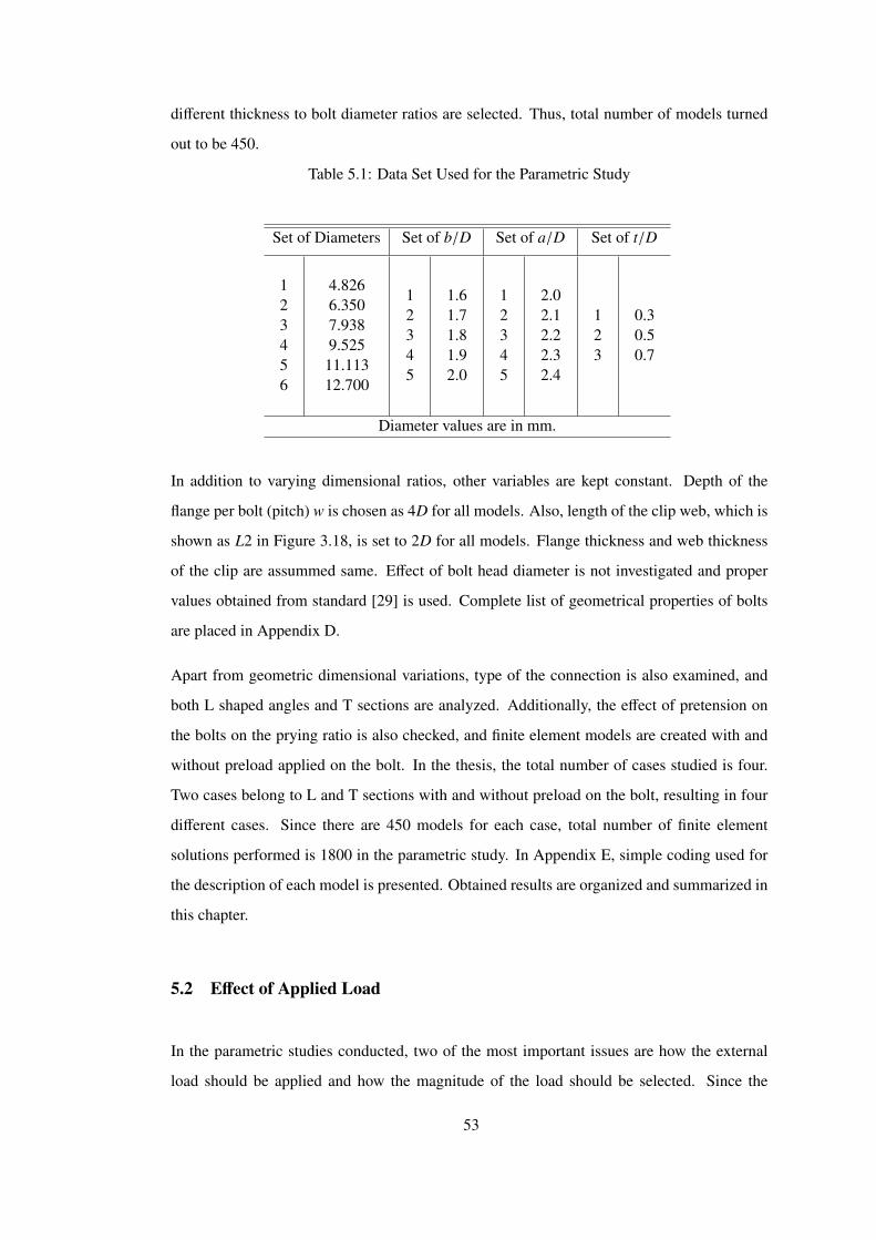
different thickness to bolt diameter ratios are selected. Thus, total number of models turned

out to be 450.

Table 5.1: Data Set Used for the Parametric Study

Set of Diameters Set of b/D Set of a/D Set of t/D

123456

4.8266.3507.9389.52511.11312.700

12345

1.61.71.81.92.0

12345

2.02.12.22.32.4

123

0.30.50.7

Diameter values are in mm.

In addition to varying dimensional ratios, other variables are kept constant. Depth of the

flange per bolt (pitch) w is chosen as 4D for all models. Also, length of the clip web, which is

shown as L2 in Figure 3.18, is set to 2D for all models. Flange thickness and web thickness

of the clip are assummed same. Effect of bolt head diameter is not investigated and proper

values obtained from standard [29] is used. Complete list of geometrical properties of bolts

are placed in Appendix D.

Apart from geometric dimensional variations, type of the connection is also examined, and

both L shaped angles and T sections are analyzed. Additionally, the effect of pretension on

the bolts on the prying ratio is also checked, and finite element models are created with and

without preload applied on the bolt. In the thesis, the total number of cases studied is four.

Two cases belong to L and T sections with and without preload on the bolt, resulting in four

different cases. Since there are 450 models for each case, total number of finite element

solutions performed is 1800 in the parametric study. In Appendix E, simple coding used for

the description of each model is presented. Obtained results are organized and summarized in

this chapter.

5.2 Effect of Applied Load

In the parametric studies conducted, two of the most important issues are how the external

load should be applied and how the magnitude of the load should be selected. Since the

53

current study involves series of cases and high number of simulation models, magnitude of

the external load must be suitable for all. First of all, instead of force, it is decided to use

negative pressure on the top surface (section of the web), as it is shown in Figure 3.10. This

way, applied force magnitude is coupled with the sectional area of the web.

However, pressure value is also very critical. Small loads result in small prying ratios, whereas

higher loads converge to a specific maximum value in case no preload is applied, as it is seen

in Figure 5.1 which corresponds to one of the sample cases. It should be noted that the current

study does not deal with the determination of stresses in the flange. But rather, the main focus

is to determine the correct prying ratio which is important in selecting the appropriate bolt

in the design process. Choosing the most critical Q/F value will be quite conservative. In

order to achieve the maximum critical ratio, pressure values in the range of 0 − 1000MPa

are applied externally on web section of Case L 1111 (see Appendix E for coding), as shown

in Figure 5.1. In that case, magnitude of the applied load varies between 0 − 27948N, since

the corresponding section area of Case L 1111 is 27.948mm2 where Aweb = wt and w = 4D.

Figure 5.1 shows that as the external force is increased, prying ratio increases, and above a

certain external force prying ratio starts to level out. However, it should be emphasized that it

is the prying ratio which more or less converges to a fixed value, not the prying load itself.

0

0.1

0.2

0.3

0.4

0.5

0.6

0.7

0.8

0.9

1

1.1

1.2

1.3

0 5000 10000 15000 20000 25000 30000

Q/F

Applied Load [N]

CASE L 1111

Figure 5.1: Effect of Applied Load on the Prying Ratio

54

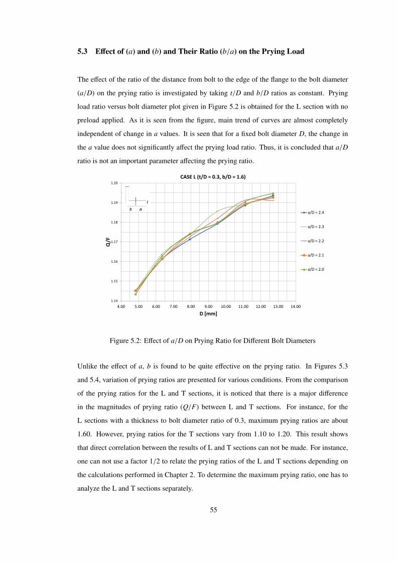
5.3 Effect of (a) and (b) and Their Ratio (b/a) on the Prying Load

The effect of the ratio of the distance from bolt to the edge of the flange to the bolt diameter

(a/D) on the prying ratio is investigated by taking t/D and b/D ratios as constant. Prying

load ratio versus bolt diameter plot given in Figure 5.2 is obtained for the L section with no

preload applied. As it is seen from the figure, main trend of curves are almost completely

independent of change in a values. It is seen that for a fixed bolt diameter D, the change in

the a value does not significantly affect the prying load ratio. Thus, it is concluded that a/D

ratio is not an important parameter affecting the prying ratio.

1.14

1.15

1.16

1.17

1.18

1.19

1.20

4.00 5.00 6.00 7.00 8.00 9.00 10.00 11.00 12.00 13.00 14.00

Q/F

D [mm]

CASE L (t/D = 0.3, b/D = 1.6)

a/D = 2.4

a/D = 2.3

a/D = 2.2

a/D = 2.1

a/D = 2.0

Figure 5.2: Effect of a/D on Prying Ratio for Different Bolt Diameters

Unlike the effect of a, b is found to be quite effective on the prying ratio. In Figures 5.3

and 5.4, variation of prying ratios are presented for various conditions. From the comparison

of the prying ratios for the L and T sections, it is noticed that there is a major difference

in the magnitudes of prying ratio (Q/F) between L and T sections. For instance, for the

L sections with a thickness to bolt diameter ratio of 0.3, maximum prying ratios are about

1.60. However, prying ratios for the T sections vary from 1.10 to 1.20. This result shows

that direct correlation between the results of L and T sections can not be made. For instance,

one can not use a factor 1/2 to relate the prying ratios of the L and T sections depending on

the calculations performed in Chapter 2. To determine the maximum prying ratio, one has to

analyze the L and T sections separately.

55

0.40

0.60

0.80

1.00

1.20

1.40

1.60

1.80

5.00 10.00 15.00 20.00 25.00 30.00 35.00

Q/F

b [mm]

CASE L (a/D = 2.0) D = 4.826 D = 6.350 D = 7.938 D = 9.525 D = 11.113 D = 12.700

t/D = 0.3

t/D = 0.5

t/D = 0.7

Figure 5.3: Effect of b on Prying Ratio for Various Diameters for L Sections

0.20

0.40

0.60

0.80

1.00

1.20

1.40

5.00 10.00 15.00 20.00 25.00 30.00 35.00

Q/F

b [mm]

CASE T (a/D = 2.0) D = 4.826 D = 6.350 D = 7.938 D = 9.525 D = 11.113 D = 12.700

t/D = 0.3

t/D = 0.5

t/D = 0.7

Figure 5.4: Effect of b on Prying Ratio for Various Diameters for T Sections

56

It is seen that for thicker flanges, when the b distance is increased, for higher bolt diameters,

slope of the prying ratio versus b lines decrease which is an indication that the effect of b

distance on the prying ratio becomes less. From Figures 5.3 and 5.4, it is clear that for larger

bolt diameters, b/D ratio is smaller in the range of b values studied. Therefore, increased

bending stiffness of the flange and smaller moment arm of the external force with respect to

the bolt axis causes prying forces to be less affected from the changes in the b distance.

On the other hand, the effect of b/a ratio is seen to be significant on the prying ratios. It

should be noted that most of the studies presented in Chapter 1 relate results of prying load to

the b/a ratio, and present it as the main part of the solution. Results of analyses performed for

L section are presented in Figures 5.5 and 5.6. In Figures 5.5 and 5.6, clouds of result points

from same t/D groups are formed. Each t/D cloud consists of 150 result points from various

diameters, b and a values. By forming graphics in this way and putting all results onto the

same graph, it is aimed to

• be able to put one single line covering all results such that drawn line may be suggested

as a conservative relation to calculate the maximum possible Q/F value for a given

configuration corresponding to the particular t/D ratio

• derive a simplified relation which depends only on b/a ratio but independent of diame-

ter and other variables such that it is simple and comparable with Douty’s and Struik’s

methods

57

0.00

0.50

1.00

1.50

2.00

2.50

0.00 0.20 0.40 0.60 0.80 1.00 1.20 1.40

Q/F

b/a

CASE L

t/D = 0.3

t/D = 0.5

t/D = 0.7

Figure 5.5: Effect of b/a on Prying Ratio for L Sections

0.00

0.40

0.80

1.20

1.60

2.00

2.40

0.00 0.10 0.20 0.30 0.40 0.50 0.60 0.70 0.80

Q/F

b'/a'

CASE L

t/D = 0.3

t/D = 0.5

t/D = 0.7

Figure 5.6: Effect of b′/a′ on Prying Ratio for L Sections

58

Results of analyses performed for Case L are presented in Figures 5.5 and 5.6. Clouds of

result points from the same t/D groups are formed. These result clouds are denser for higher

t/D ratios. In another words, effect of change in the b/a ratio is less when the bending capacity

of the flange is increased. On the other hand, ineffectiveness of a simply causes b to dominate

the effect of b/a ratio, and it is seen that in general prying ratio (Q/F) increases with the b/a

ratio.

In Figures 5.5 and 5.6, simplified relations of ”Struik L” and ”Douty L” for the prying ratios

are simply twice of the original formulations of Douty and Struik obtained for T sections (see

Equations 2.28 and 2.29). However, it is noted that multiplying the simplified prying ratios

of T sections by two and adopting them for L sections is not a suitable assumption. Unless

the t/D ratio is equal to or higher than 0.7, Douty’s approach cannot determine the results

obtained from finite element analysis. Similarly, Struik’s approach cannot even cover the case

of t/D = 0.7.

Apart from analytical formulations of Douty and Struik, simple relations for prying ratios can

be also obtained from Figures 5.5 and 5.6 for better estimation of Q/F for different t/D ratios.

For instance, in Figure 5.5, line of 2b/a covers all results for the t/D ratio of 0.3. However, it

might be too conservative to use 2b/a for t/D ratios of 0.5 or 0.7. Therefore, defining separate

simplified relations covering all the prying ratio results for each t/D ratio is considered to be

more appropriate. Equation 5.1 gives the proposed simplified relations which give prying

ratios applicable for three different t/D ratios.

(QF

)L

=

2b/a, t/D = 0.3

b/a, t/D = 0.5

3b/4a, t/D ≥ 0.7

(5.1)

Similar approach may be repeated for Figure 5.6 which is based on b′/a′ ratios. Simplified

expressions for the prying ratios are given in Equation 5.2 where a′ = a+D/2 and b′ = b−D/2.

(QF

)L

=

16b′/5a′, t/D = 0.3

12b′/7a′, t/D = 0.5

9b′/7a′, t/D ≥ 0.7

(5.2)

59

0.00

0.40

0.80

1.20

1.60

2.00

0 0.2 0.4 0.6 0.8 1 1.2 1.4

Q/F

b/a

CASE T

t/D = 0.3

t/D = 0.5

t/D = 0.7

Figure 5.7: Effect of b/a on the Prying Ratio for T Sections

0.00

0.40

0.80

1.20

1.60

2.00

0 0.1 0.2 0.3 0.4 0.5 0.6 0.7 0.8

Q/F

b'/a'

CASE T

t/D = 0.3

t/D = 0.5

t/D = 0.7

Figure 5.8: Effect of b′/a′ on the Prying Ratio for T Sections

60

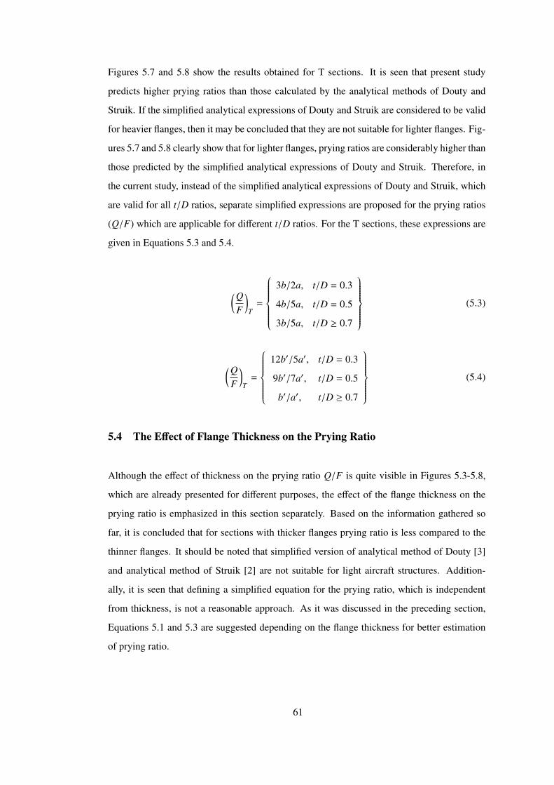
Figures 5.7 and 5.8 show the results obtained for T sections. It is seen that present study

predicts higher prying ratios than those calculated by the analytical methods of Douty and

Struik. If the simplified analytical expressions of Douty and Struik are considered to be valid

for heavier flanges, then it may be concluded that they are not suitable for lighter flanges. Fig-

ures 5.7 and 5.8 clearly show that for lighter flanges, prying ratios are considerably higher than

those predicted by the simplified analytical expressions of Douty and Struik. Therefore, in

the current study, instead of the simplified analytical expressions of Douty and Struik, which

are valid for all t/D ratios, separate simplified expressions are proposed for the prying ratios

(Q/F) which are applicable for different t/D ratios. For the T sections, these expressions are

given in Equations 5.3 and 5.4.

(QF

)T

=

3b/2a, t/D = 0.3

4b/5a, t/D = 0.5

3b/5a, t/D ≥ 0.7

(5.3)

(QF

)T

=

12b′/5a′, t/D = 0.3

9b′/7a′, t/D = 0.5

b′/a′, t/D ≥ 0.7

(5.4)

5.4 The Effect of Flange Thickness on the Prying Ratio

Although the effect of thickness on the prying ratio Q/F is quite visible in Figures 5.3-5.8,

which are already presented for different purposes, the effect of the flange thickness on the

prying ratio is emphasized in this section separately. Based on the information gathered so

far, it is concluded that for sections with thicker flanges prying ratio is less compared to the

thinner flanges. It should be noted that simplified version of analytical method of Douty [3]

and analytical method of Struik [2] are not suitable for light aircraft structures. Addition-

ally, it is seen that defining a simplified equation for the prying ratio, which is independent

from thickness, is not a reasonable approach. As it was discussed in the preceding section,

Equations 5.1 and 5.3 are suggested depending on the flange thickness for better estimation

of prying ratio.

61

0.20

0.40

0.60

0.80

1.00

1.20

1.40

4 5 6 7 8 9 10 11 12 13 14

Q/F

D [mm]

CASE L (b/D = 1.6, a/D = 2.0)

t/D = 0.3

t/D = 0.5

t/D = 0.7

Figure 5.9: Effect of Thickness on the Prying Ratio for L Sections

Effect of thickness of the flange on the prying ratio is presented in Figure 5.9 as an additional

sample study to support the results presented before. From Figure 5.9, it can be seen that

prying ratio (Q/F) decreases when the flange thickness to the bolt diameter ratio (t/D) is

increased. It is also seen that for fixed a/D and b/D ratios, prying ratio is almost indepen-

dent of the bolt diameter D. Prying ratio versus bolt diameter curves become flatter as the

bolt diameter is increased. Figure 5.9 shows that flange thickness is an important parameter

affecting the prying ratio. Especially, for sections with thinner flanges, prying ratio is higher,

and it is not independent of the t/D ratio. This means that simplified relations for the prying

ratio, such as the ones proposed by Douty and Struik, which do not have t/D dependency are

not very reliable. It is recommended that especially, for thinner sections, which are frequently

used in aerospace structures, high fidelity solutions must be performed for the calculation of

the prying loads.

62

5.5 The Effect of Preload on the Prying Ratio

Application of preload on bolt changes the bolt and prying loads as shown in Figure 5.10. In

Figure 5.10, dashed line shows no prying case for which the bolt load and the external load

are equal to each other. The other curves in Figure 5.10 show the bolt load and the prying load

for the cases with and without preload on the bolt for model L1111. The model definitions

are given in Appendix E.

0

5000

10000

15000

20000

25000

30000

35000

40000

45000

0 2000 4000 6000 8000 10000 12000 14000 16000 18000 20000

LOAD

[N]

APPLIED LOAD [N]

BOLT LOAD for MODEL L1111 NO PRYING, NO PRELOAD

NO PRYING, PRELOADED

BOLT LOAD w/o PRELOAD on BOLT (LP1111)

BOLT LOAD w/o PRELOAD on BOLT (L1111)

PRYING LOAD w/o PRELOAD on BOLT (LP1111)

PRYING LOAD w/o PRELOAD on BOLT (L1111)

Figure 5.10: Bolt Load and Prying Load Variation by Applied Load for Model L1111

When the case without preload is examined, it is seen that bolt load curve starts from zero

initial load and smoothly increases just like the prying. On the other hand, for the case with

the preload, bolt load curve starts from initial preload value which is about 3973 N for the

given sample case. Prying load curve again starts from initial value of zero and slowly creates

an offset with respect to prying load curve of no preload case until the applied load reaches

the load at which the flange separation at the bolt location occurs. Although it is not easy to

determine exact location on the graph where complete separation of flange around the bolt

region occurs, after that point it might be said that prying curves remain almost parallel to

each other which is quite suitable for linear static analysis.

63

Figure 5.11 presents the prying ratio results for the L section with preload applied on the bolt.

As it is seen, cloud of prying ratio results show a similar pattern as the no preload case for

which the similar plot is given in Figure 5.5.

0

0.5

1

1.5

2

2.5

3

0 0.2 0.4 0.6 0.8 1 1.2 1.4

Q/F

b/a

CASE LP

t/D 0.3

t/D 0.5

t/D 0.7

Figure 5.11: Effect of b/a on the Prying Ratio for L Sections with Preload Applied on theBolt

According to the results in Figure 5.11, suggested equations can be given as

(QF

)LP

=

13b/6a, t/D = 0.3

11b/10a, t/D = 0.5

4b/5a, t/D ≥ 0.7

(5.5)

Figure 5.12 gives the variation of the effect of preload on the prying ratio with the bolt diam-

eter and for different thickness to bolt diameter ratios for L Sections. From Figure 5.12, it is

clear that prying ratios are higher when preload is applied. In addition, the effect of preload

on the prying ratio is higher for low t/D ratios. So, for thinner flanges preload affects the

prying ratio more, which makes sense. As the t/D ratio is increased, implying thicker flanges,

the effect of bolt preload on the prying ratio decreases. From the trend seen in Figure 5.12, it

can be commented that if the t/D ratio is increased further, the effect of bolt preload on the

prying ratio will be almost non-existent. Figure 5.12 also shows that for higher t/D ratios,

prying ratio versus bolt diameter curves are almost flat which is an indication that prying ra-

64

tio is almost independent of the bolt diameter. Therefore, one can confidently conclude that

thickness of the flange is an important parameter affecting the prying ratio, and for thinner

flanges the effect of preload on the prying ratio is high and for thicker flanges the effect of

preload on the prying ratio is low.

0.20

0.40

0.60

0.80

1.00

1.20

1.40

4 6 8 10 12 14

Q/F

D [mm]

CASE L (b/D = 1.6, a/D = 2.0)

LP, t/D = 0.3 L, t/D = 0.3 LP, t/D = 0.5 L, t/D = 0.5 LP, t/D = 0.7 L, t/D = 0.7

Figure 5.12: Variation of the Effect of Preload on the Prying Ratio with the Bolt Diameter forDifferent Thickness to Bolt Diameter Ratios - L Sections

65

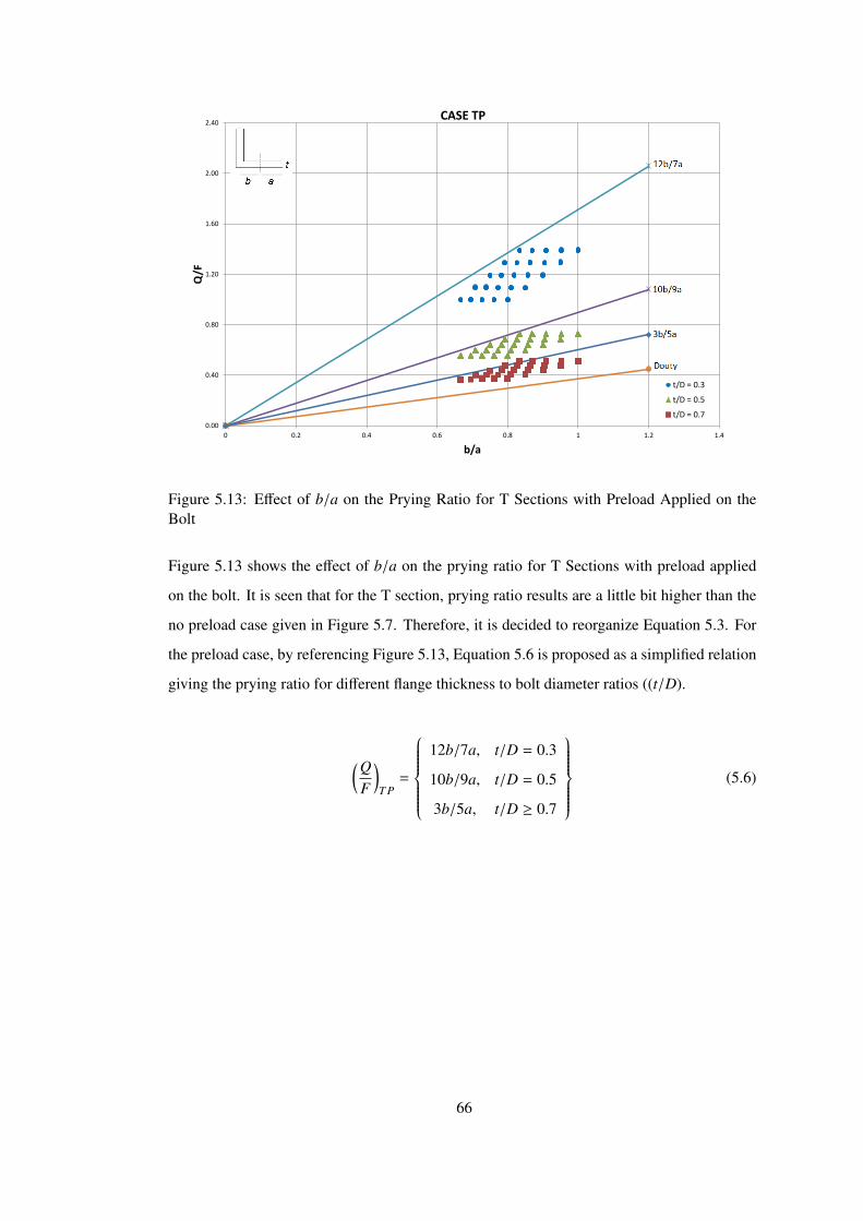
0.00

0.40

0.80

1.20

1.60

2.00

2.40

0 0.2 0.4 0.6 0.8 1 1.2 1.4

Q/F

b/a

CASE TP

t/D = 0.3

t/D = 0.5

t/D = 0.7

Figure 5.13: Effect of b/a on the Prying Ratio for T Sections with Preload Applied on theBolt

Figure 5.13 shows the effect of b/a on the prying ratio for T Sections with preload applied

on the bolt. It is seen that for the T section, prying ratio results are a little bit higher than the

no preload case given in Figure 5.7. Therefore, it is decided to reorganize Equation 5.3. For

the preload case, by referencing Figure 5.13, Equation 5.6 is proposed as a simplified relation

giving the prying ratio for different flange thickness to bolt diameter ratios ((t/D).

(QF

)T P

=

12b/7a, t/D = 0.3

10b/9a, t/D = 0.5

3b/5a, t/D ≥ 0.7

(5.6)

66

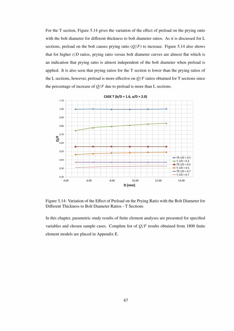
For the T section, Figure 5.14 gives the variation of the effect of preload on the prying ratio

with the bolt diameter for different thickness to bolt diameter ratios. As it is discussed for L

sections, preload on the bolt causes prying ratio (Q/F) to increase. Figure 5.14 also shows

that for higher t/D ratios, prying ratio versus bolt diameter curves are almost flat which is

an indication that prying ratio is almost independent of the bolt diameter when preload is

applied. It is also seen that prying ratios for the T section is lower than the prying ratios of

the L sections, however, preload is more effective on Q/F ratios obtained for T sections since

the percentage of increase of Q/F due to preload is more than L sections.

0.20

0.30

0.40

0.50

0.60

0.70

0.80

0.90

1.00

1.10

4.00 6.00 8.00 10.00 12.00 14.00

Q/F

D [mm]

CASE T (b/D = 1.6, a/D = 2.0)

TP, t/D = 0.3 T, t/D = 0.3 TP, t/D = 0.5 T, t/D = 0.5 TP, t/D = 0.7 T, t/D = 0.7

Figure 5.14: Variation of the Effect of Preload on the Prying Ratio with the Bolt Diameter forDifferent Thickness to Bolt Diameter Ratios - T Sections

In this chapter, parametric study results of finite element analyses are presented for specified

variables and chosen sample cases. Complete list of Q/F results obtained from 1800 finite

element models are placed in Appendix E.

67

CHAPTER 6

DISCUSSIONS AND CONCLUSIONS

In this thesis, prying effect on bolts used in tension clip connections and shear clip stringer

connections are investigated for both L and T sections. Firstly, in order to understand the

behavior of the tensile connections clearly, simple free body diagrams are drawn and basic

equilibrium equations are written. Through these simple equations, basic prying force ratios

are obtained. Additionally, variations of bolt load, prying load and contact forces between

flange and base plate around the bolt region is explained by referencing different studies from

the literature.

Different approaches in obtaining the prying load are presented from the literature. Bruhn and

Niu represent the aeronautical point of view about the prying load. Both of them emphasize

the impossibility of exact calculation of prying ratios via analytical approaches. It is the fact

that aircraft manufacturers conduct series of experiments for various cases and fit curves to

the results so that useful reference data is obtained. On the other hand, Douty and McGuire,

Agerskov and Struik and de Back, who are the representatives of the civil engineering point

of view given in this thesis, aimed to derive analytical expressions which estimate the prying

load as accurately as possible. In some cases, results of these approaches are also compared

with the series of experiments conducted by researchers such as Agerskov.

After the introduction of the analytical studies conducted in the literature, design consider-

ations of the current study are presented. Simplified expressions of Douty and Struik are

decided to be compared with results of finite element analyses. Comparisons are performed

in a design space which is narrowed down according to the limitations discussed by Struik

and general practice adopted in aircraft structural design.

68

Finite element models prepared for the prying load calculations are introduced in Chapter

3. Boundary conditions, loads and material properties are described in detail. Methodology

followed to apply preload on the bolt and, and the method followed to obtain prying ratios

from finite element results performed in Abaqus, are explained. Mesh sensitivity analysis is

performed for a chosen configuration, and it is decided to use at least four elements through

the thickness of the flange. Parametric modeling process is described and geometrical dimen-

sions, which are controlled in the parametric modeling process, are presented. Additionally,

developed Phyton algorithm is given, and the script is placed in Appendix A.

Reliability of the results obtained by the finite element solution is checked by comparing

the results with the experimental and analytical results presented by Agerskov, Douty and

AISC [1]. Analytical results of Agerskov, Douty, AISC and experimental results of Agerskov

are compared with the results obtained from the finite element models prepared according

to the original test specimen properties. Based on the comparison of the results, it is seen

that finite element results are in good agreement with analytical results. Results of methods

presented by Douty and Agerskov have maximum difference of 14% with respect to the finite

element analyses results of the present study. On the other hand, prying ratios of AISC have

a maxiumum difference of 53% with respect to the results of Douty and Agerskov. Higher

discrepancy of the prying ratios of AISC is considered to be acceptable, because as Agerskov

states, AISC’s method is too conservative. In addition, comparison of test results of Agerskov

and finite element results is also presented. It is seen that finite element results, obtained in

the current study, have maximum difference of 9% with respect to the test results.

Parametric study of series of models are described with the data set used in Chapter 5. Six

different frequently used bolt diameters are chosen from the standards. Geometric values of a

and b are set in terms of their ratios to the bolt diameter, and five different ratios are selected

for each. Additionally, flange thickness is taken into consideration by the t/D ratio which the

ratio of the flange thickness to the bolt diameter, and three different flange thickness to the

bolt diameter ratios are chosen in the parametric study. Apart from varying the dimensions

described, other dimensions are chosen again depending on the bolt diameter ratio. In all

models, flange depth of the clip per bolt (w) is taken as 4D, and the height of the clip web is

taken as 2D. All these geometrical dimensions are used for both L and T sections, and for

the case studies with and without bolt preload. As a result, 1800 finite element analyses are

performed in total.

69

In order to obtain conservative Q/F ratios, applied load is selected quite large since the prying

ratio converges as the applied load is increased. Collected results of 1800 models are reor-

ganized for understanding the effect of different variables on the prying load. Effects of a, b,

b/a and t/D on the prying ratio are investigated.

It is pointed by Struik that the assumption of prying load acting as a line load at the tip of the

flange is valid only for limited range of a values. However, comparing the results obtained for

various a values showed that a is not much effective on the prying ratio Q/F in the selected

interval and design space.

On the other hand, b is determined to be one of the most effective variables on the prying ratio.

It is seen that prying ratios increase rapidly with the b value. It is also concluded that effect

of b on the prying ratio depends on the thickness of the flange. When the flange thickness is

increased, the effectiveness of b on the prying ratio becomes less since the bending stiffness

of flange increases with the cube of the thickness, whereas moment arm of eccentric loads

that try to bend the flange is proportional to b only.

b/a ratio is also considered to be a very important parameter on the prying ratio, since re-

searchers like Douty and Struik focused on this ratio, and presented their analytical results

using this ratio. In the current study, results of finite element analyses, which belong to same

cases are collected on the same graphics. Linear lines depending on the b/a ratios are drawn

such that they cover complete results of common t/D values. This way, comparison between

analytical calculations and finite element analyses results is performed. For both L and T sec-

tions, it is seen that analytical methods suggested by Douty and Struik are not applicable to

light flange connections, which are also considered in this study. Due to this fact, it is decided

to propose simple relations in order to obtain prying ratio depending on b/a and t/D ratios.

Thickness of the clip flange is another important variable in the determination of the prying

load ratio. It is observed that increasing flange thickness decreases the prying ratio. Especially

for light flange connections, simplified analytical formulations which do not take t/D ratio

into account are not reliable.

Finally, effect of preload on the prying ratio is investigated. It is seen that preload increases

the prying ratio, and this increase is determined to be more effective on T sections than L

sections. Similar to the cases without preload, effect of b/a on the prying ratio is investigated,

70

and simplified relations for the prying ratio are proposed for both L and T sections with bolt

preload taken into account.

In the future, the current study may be extended by increasing the design space chosen. De-

sign space can be expanded by adding different bolt diameter , a, b and t values which are

not covered in the present study. On the other hand, the developed script can be modified, so

that it can be applied to series of aerospace sub-structure problems which are examined by

the manufacturers and designers of aerospace structures. Algorithm can be adapted such that

it reads all geometrical constraints and load requirements, it combines these inputs and per-

forms preliminary design and analysis automatically. According to the results obtained, the

developed script may optimize the structural configuration such as dimensions, bolt selection

and positioning, and material. However, this kind of automatic process need to be verified by

the tests and finite element analyses. Only after the verification phase, the developed script

may be considered as a reliable and faster design and analysis tool.

Although stresses beyond the yield limit is an unwanted case for most of the aircraft structures,

current study may be improved by taking material non-linearity into account. Thus, bolt

load variation under prying effect may be investigated more realistically. It is noted that

under preload, the stress level in the flange may exceed the yield limit. Therefore, material

nonlinearity should be taken into account in the calculation of the prying loads, determination

of the full field stress distribution in the clip.

Another future study could be on the determination of the prying force experimentally. A

special test set-up may be designed with bolts having embedded strain gages. With such a test

set-up, first bolt forces can be determined as accurately as possible, and then prying force can

be determined. It is considered that determination of the prying force experimentally is a very

worthwhile effort.

Furthermore, effect of the head diameter of the bolt, washer diameter and radius fillers on the

prying ratio may also be investigated. It is noted that radius filler is an effective solution in

reducing the effect of prying force on the critical tension connections.

71

REFERENCES

[1] Agerskov, H., “High Strength Bolted Connections Subject to Prying,” Journal of theStructural Division, Vol. 102, 1979, pp. 161 – 175.

[2] Kulak, G.; Fisher, J. W. and Struik, J. H. A., Guide to Design Criteria for Bolted andRiveted Joints, John Wiley and Sons, New York,, 1974.

[3] Douty, R. T.; McGuire, W., “High Strength Bolted Moment Connections,” Journal ofthe Structural Division, Vol. ST2, 1965, pp. 101 – 128.

[4] Krishnamurthy, N.; Thambiratnam, D. P., “Finite Element Analysis of Column BasePlates,” Computers and Structures, Vol. 34, No. 2, 1990, pp. 215 – 223.

[5] Nair, R.S.; Birkemoe, P. and Munse, W., “Behavior of Bolts in Tee-Connections Subjectto Prying Action,” Journal of the Structural Division, Vol. 353, 1969, pp. 161 – 175.

[6] Bruhn, E., Analysis and Design of Airplane Structures, Tri-State Offset Co., 1949.

[7] Niu, M. C. Y., Airframe Stress Analysis and Sizing, Hong Kong Conmilit Press Ltd.,2007.

[8] Kato, B.; McGuire, W., “Analysis of T-Stub Flange-to-Column Connections,” Journalof Structural Division, Vol. ST5, 1973, pp. 865–888.

[9] Steel Construction Manual, 14th Edition, AISC, USA, 2011.

[10] Thornton, W., “Prying Action - A General Treatment,” Engineering Journal, Vol. 22,No. 2, 1985, pp. 67–75.

[11] Swanson, J., “Ultimate Strength Prying Models for Bolted T-Stub Connections,” Engi-neering Journal, Vol. 39, No. 3, 2002, pp. 136–147.

[12] Nair, R.S.; Birkemoe, P. and Munse, W., “High Strength Bolts Subjected to Tension andPrying,” Journal of the Structural Division, Vol. 100, 1974.

[13] Struik, J. H. A.; de Back, J., “Tests on Bolted T-Stub with Respect to a Bolted Beam-Column Connections,” Tech. Rep. 6-69-13, Stevin Labratory, TU-DELFT, 1969.

[14] Krishnamurthy, N., “Experimental Validation of End-Plate Connection Design,” Tech.rep., AISC, 1979.

[15] Kennedy, N.A.; Vinnakota, S. and Sherbourne, A., “The Split-Tee Analogy inBolted Splices and Beam-Column Connections,” Joints in Structural Steelwork, 1981,pp. 2.138–2.157.

[16] Jaspart, J. P. and Maquoi, R., editors, Plastic Capacity of End-Plate and Flange CleatedConnections - Predictions and Design Rules, Pittsburgh, PA,, April 1991, 2nd Interna-tional Workshop on Connections in Steel Structures: Behavior, Strength and Design.

72

[17] Kukreti, Anant R., M. T. M. and Ghassemieh, M., “Finite Element Modeling of LargeCapacity Stiffenes Steel Tee-Hanger Connections,” Computers and Structures, Vol. 32,No. 2, 1989, pp. 409 – 422.

[18] Chasten, C., “Prying and shear in end-plate connection design,” Journal of StructureEngineering, ASCE, Vol. 118, 1992, pp. 77 – 89.

[19] Maggi, Y., Goncalves, R., Leon, R., and Ribeiro, L., “Parametric analysis of steel boltedend plate connections using finite element modeling,” Journal of Constructional SteelResearch, Vol. 61, No. 5, 2005, pp. 689 – 708.

[20] Komuro, M.; Kishi, N. and Ahmed, A., “Elasto-Plastic Finite Element Analysis of Pry-ing of Top and Seat-Angle Connections,” Advances in Engineering Structures, Mechan-ics and Construction, Vol. 140 of Solid Mechanics and Its Applications, 2006, pp. 289–301.

[21] ESDU, “Analysis of pretensioned bolted joints subject to tensile (separating) forces,”Tech. Rep. 85021, ESDU, 1985.

[22] ESDU, “Strength of angles and club-foot fittings (transmitting tensile loads),” Tech. Rep.84039, ESDU, 1986.

[23] ASCE, Commentary on Plastic Design, 1971, Manual 41.

[24] Schutz, F. W., editor, Strength of Moment Connections Using High Tensile Bolts. Natl.Engrg. Conf., AISC, New York, 1959.

[25] Agerskov, H., “Analysis of Bolted Connections Subject to Prying,” Journal of the Struc-tural Division, Vol.102, 1979, pp. 1851 – 1855.

[26] Timoshenko, S.; Woinowsky-Krieger, S., Theory of Plates and Shells, 10th, EngineeringSocieties Monographs, McGraw-Hill, USA, 1959.

[27] Abaqus Analysis User’s Manual, Providence, RI,USA, 2009.

[28] Budynas and Nisbett, Shigley’s Mechanical Engineering Design, McGraw-Hill, 8th ed.,2006.

[29] AIAA, N. A. S. C., AIA/NAS 609 62, 1962.

[30] Abaqus Scripting User’s Manual, Providence, RI,USA, 2011.

[31] Overvelde, J., Learn Abaqus Script in One Hour, http://www.overvelde.com, 2010, lastvisit: 27.02.2012.

[32] Federal Aviation Administration (FAA), Metallic Materials Properties Developmentand Standardization (MMPDS) - 03, 2006.

73

APPENDIX A

PHYTON SCRIPTING

A.1 Suggestions for Phyton Scripting on Abaqus

Best way to start Abaqus scripting is creation of model manually at the beginning. It is

suggested to create target model with least mouse move and selection since every move

is recorded by the session files with *.rpy. When the model is completed, one may check

abaqus.rpy file recorded in the same folder of related model file (*.cae). Instead of creating a

Phyton script from the beginning, modifying abaqus.rpy file is easier approach. Besides, it is

strongly suggested to take a look at Overvelde’s work [31]

A.2 Script Used for Parametric Study

sizer arraycontainsgeometricvaluesandrelatedloads :

sizer D = [4.826, 6.35, 7.938, 9.525, 11.113, 12.7]

sizer T = [0.3, 0.5, 0.7]

sizer B = [1.6, 1.7, 1.8, 1.9, 2.0]

sizer A = [2.0, 2.1, 2.2, 2.3, 2.4]

length D = len(sizer D)

length B = len(sizer B)

length A = len(sizer A)

length T = len(sizer T )

74

f orloop count Dinrange(1, length D + 1) :

f orloop count Binrange(1, length B + 1) :

f orloop count Ainrange(1, length A + 1) :

f orloop count T inrange(1, length T + 1) :

S tringerDetailedDimensioning :

D(DIAMET ER)

sizeD = sizer D[loop count D − 1]

T (T HICKNES S )

sizeT = sizeD ∗ sizer T [loop count T − 1]

sizeL2 = sizeD ∗ 2.0

Re f erringtoS tringer.xlsx

sizeA pr = (sizeL1 − sizeT/2)/1.6582

sizeA = sizeD ∗ sizer A[loop count A − 1]

sizeB = sizeD ∗ sizer B[loop count B − 1]

sizeL1 = sizeA + sizeB

w(PITCH)

sizeW = 4 ∗ sizeD

print′MODELisREADY f orRunNumber%s%s%s%s′%(loop count D, loop count B, loop count A, loop count T )

f romabaqusimport∗

f romabaqusConstantsimport∗

f romcaeModulesimport∗

f rompartimport∗

f rommaterialimport∗

f romsectionimport∗

f romassemblyimport∗

f romstepimport∗

f rominteractionimport∗

75

f romloadimport∗

f rommeshimport∗

f rom jobimport∗

f romsketchimport∗

f romvisualizationimport∗

f romconnectorBehaviorimport∗

f romdriverUtilsimportexecuteOnCaeS tartup

executeOnCaeS tartup()

RenameModel − 1toPRYING MODEL :

mdb.models.changeKey( f romName =′ Model − 1′, toName =′ PRYING MODEL′)

BasicS ketchwithoutdetaileddimensions :

s = mdb.models[′PRYING MODEL′].ConstrainedS ketch(name =′ pro f ile ′,

sheetS ize = 200.0)

g, v, d, c = s.geometry, s.vertices, s.dimensions, s.constraints

s.setPrimaryOb ject(option = S T ANDALONE)

s.Line(point1 = (0.0, 0.0), point2 = (0.0, 15.0))

s.VerticalConstraint(entity = g[2], addUndoS tate = False)

s.Line(point1 = (0.0, 15.0), point2 = (5.0, 15.0))

s.HorizontalConstraint(entity = g[3], addUndoS tate = False)

s.PerpendicularConstraint(entity1 = g[2], entity2 = g[3], addUndoS tate = False)

s.Line(point1 = (5.0, 15.0), point2 = (5.0, 5.0))

s.VerticalConstraint(entity = g[4], addUndoS tate = False)

s.PerpendicularConstraint(entity1 = g[3], entity2 = g[4], addUndoS tate = False)

s.Line(point1 = (5.0, 5.0), point2 = (15.0, 5.0))

s.HorizontalConstraint(entity = g[5], addUndoS tate = False)

s.PerpendicularConstraint(entity1 = g[4], entity2 = g[5], addUndoS tate = False)

s.Line(point1 = (15.0, 5.0), point2 = (15.0, 0.0))

s.VerticalConstraint(entity = g[6], addUndoS tate = False)

s.PerpendicularConstraint(entity1 = g[5], entity2 = g[6], addUndoS tate = False)

76

s.Line(point1 = (15.0, 0.0), point2 = (0.0, 0.0))

s.HorizontalConstraint(entity = g[7], addUndoS tate = False)

s.PerpendicularConstraint(entity1 = g[6], entity2 = g[7], addUndoS tate = False)

Constraint :

s.FixedConstraint(entity = v[0])

L1(WIDT H) = (a + b + t)

s.ObliqueDimension(vertex1 = v[5], vertex2 = v[0], textPoint = (7.41244888305664,

−2.46644592285156), value = sizeL1)

t(T HICKNES S )

s.ObliqueDimension(vertex1 = v[1], vertex2 = v[2], textPoint = (3.76505279541016,

19.2617416381836), value = sizeT )

s.ObliqueDimension(vertex1 = v[4], vertex2 = v[5], textPoint = (18.7076072692871,

2.58388900756836), value = sizeT )

L2(HEIGHT )

s.ObliqueDimension(vertex1 = v[0], vertex2 = v[1], textPoint = (−3.2944221496582,

9.98321914672852), value = sizeL2)

p = mdb.models[′PRYING MODEL′].Part(name =′ S TRINGER′, dimensionality = T HREE D,

type = DEFORMABLE BODY)

p = mdb.models[′PRYING MODEL′].parts[′S TRINGER′]

p.BaseS olidExtrude(sketch = s, depth = sizeW)

S tringerPartitioning −CuttingHole

c = p.cells

v = p.vertices

f , e, d = p. f aces, p.edges, p.datums

distance1 == w/2(HALFPITCH)

77

distance2 == a(Distance f romTip)

sizeWo2 = sizeW/2.0

p.HoleThruAllFromEdges(plane = f [3], edge1 = e[12], edge2 = e[10], planeS ide = S IDE1,

diameter = sizeD, distance1 = sizeWo2, distance2 = sizeA)

BasePartition

pickedCells = c.getS equenceFromMask(mask = (′[#1]′, ), )

p.PartitionCellByPlanePointNormal(point = v[8], normal = e[9], cells = pickedCells)

pickedCells = c.getS equenceFromMask(mask = (′[#2]′, ), )

p.PartitionCellByPlanePointNormal(point = v[0], normal = e[4], cells = pickedCells)

FacePartition

t = p.MakeS ketchTrans f orm(sketchPlane = f . f indAt(coordinates = (sizeT, sizeT,

1.0)), sketchU pEdge = e. f indAt(coordinates = (sizeT, sizeT, sizeW)),

sketchPlaneS ide = S IDE1, origin = (sizeT, sizeT, 0.0))

s = mdb.models[′PRYING MODEL′].ConstrainedS ketch(name =′ pro f ile ′,

sheetS ize = 117.74, gridS pacing = 2.94, trans f orm = t)

s.setPrimaryOb ject(option = S UPERIMPOS E)

p.pro jectRe f erencesOntoS ketch(sketch = s, f ilter = COPLANAR EDGES )

WasherDiameterDecision

s.CircleByCenterPerimeter(center = (sizeWo2, sizeB − sizeT/2), point1 = (sizeWo2 + 0.825 ∗ sizeD, sizeB − sizeT/2))

pickedFaces = f . f indAt(((sizeT + 1, sizeT, 1.0), ))

p.PartitionFaceByS ketch(sketchU pEdge = e. f indAt(coordinates = (sizeT + 1, sizeT,

sizeW)), f aces = pickedFaces, sketch = s)

s.unsetPrimaryOb ject()

delmdb.models[′PRYING MODEL′].sketches[′ pro f ile ′]

78

Materials :

mdb.models[′PRYING MODEL′].Material(name =′ AL′)

mdb.models[′PRYING MODEL′].materials[′AL′].Elastic(table = ((72000.0, 0.33), ))

mdb.models[′PRYING MODEL′].Material(name =′ AL BOLT ′)

mdb.models[′PRYING MODEL′].materials[′AL BOLT ′].Elastic(table = ((186000.0, 0.27), ))

S ections :

mdb.models[′PRYING MODEL′].HomogeneousS olidS ection(material =′ AL′, name =

′S ection − 1′, thickness = None)

mdb.models[′PRYING MODEL′].HomogeneousS olidS ection(material =′ AL BOLT ′, name =

′S ection − Bolt′, thickness = None)

AssignS ection

cells = p.cells.getS equenceFromMask(mask = (′[#71]′, ), )

region = regionToolset.Region(cells = cells)

p.S ectionAssignment(region = region, sectionName =′ S ection − 1′, o f f set = 0.0,

o f f setType = MIDDLE S URFACE, o f f setField =′′,

thicknessAssignment = FROM S ECT ION)

Mesh

FirstS eed

seed size = min(2., sizeT/5)

p.seedPart(deviationFactor = 0.1, size = seed size)

MeshControl

pickedRegions = c. f indAt(((sizeT + 1, sizeT, 1.0), ))

p.setMeshControls(regions = pickedRegions, algorithm = MEDIAL AXIS )

CreateMesh

p = mdb.models[′PRYING MODEL′].parts[′S TRINGER′]

p.generateMesh()

Regenerate

p.regenerate()

79

Part1 − S TRINGERiscreated,meshedandsoready!

print′Part1 − S TRINGERiscreated′

CreatingRigidPlate

s2 = mdb.models[′PRYING MODEL′].ConstrainedS ketch(name =′ pro f ile ′,

sheetS ize = 200.0)

s2.setPrimaryOb ject(option = S T ANDALONE)

s2.Line(point1 = (−1.0,−0.01), point2 = (sizeL1 + 2,−0.01))#CHANGE

p2 = mdb.models[′PRYING MODEL′].Part(name =′ RIGID PLAT E′, dimensionality = T HREE D,

type = ANALYT IC RIGID S URFACE)

p2 = mdb.models[′PRYING MODEL′].parts[′RIGID PLAT E′]

p2.AnalyticRigidS ur f Extrude(sketch = s2, depth = 2 ∗ sizeW + 2)

s2.unsetPrimaryOb ject()

Part2 − RIGIDPLAT Eiscreated

print′Part2 − RIGIDPLAT Eiscreated′

CreatingBolt[Headheight = sizeD, length = −1 ∗ sizeT ]

size Nut = sizeD

s3 = mdb.models[′PRYING MODEL′].ConstrainedS ketch(name =′ pro f ile ′,

sheetS ize = 50.0)

g3, v3, d3, c3 = s3.geometry, s3.vertices, s3.dimensions, s3.constraints

s3.setPrimaryOb ject(option = S T ANDALONE)

s3.ConstructionLine(point1 = (0.0,−25.0), point2 = (0.0, 25.0))

s3.FixedConstraint(entity = g3[2])

s3.Line(point1 = (0.0,−1 ∗ sizeT ), point2 = (0.0, sizeT + size Nut))

s3.Line(point1 = (0.0, sizeT + size Nut), point2 = (0.825 ∗ sizeD, sizeT + size Nut))

s3.Line(point1 = (0.825 ∗ sizeD, sizeT + size Nut), point2 = (0.825 ∗ sizeD, sizeT ))

s3.Line(point1 = (0.825 ∗ sizeD, sizeT ), point2 = (sizeD, sizeT ))

s3.Line(point1 = (sizeD/2.0, sizeT ), point2 = (sizeD/2.0,−1 ∗ sizeT ))

80

s3.Line(point1 = (sizeD/2.0,−1 ∗ sizeT ), point2 = (0.0,−1 ∗ sizeT ))

p3 = mdb.models[′PRYING MODEL′].Part(name =′ BOLT ′, dimensionality = T HREE D,

type = DEFORMABLE BODY)

p3 = mdb.models[′PRYING MODEL′].parts[′BOLT ′]

p3.BaseS olidRevolve(sketch = s3, angle = 360.0, f lipRevolveDirection = OFF)

s3.unsetPrimaryOb ject()

PartitioningtheBolt f orBCapplication

CreateDatumPlane

p3.DatumPlaneByPrincipalPlane(principalPlane = XZPLANE, o f f set = 0.0)

Partition

p3.PartitionCellByDatumPlane(cells = p3.cells. f indAt(((0.0, 0.0, 0.0), )), datumPlane = p3.datums[2])

Partition f orisoparametricmesho f head

p3.PartitionCellByExtendFace(cells =

p3.cells. f indAt(((0.0, 0.5, 0.0), )), extendFace =

p3. f aces. f indAt((0.0, sizeT, 0.1), ))

Partition f orpreloadapplication

CreateDatumPlane

p3.DatumPlaneByPrincipalPlane(principalPlane = XZPLANE, o f f set = sizeT )

Partition

p3.PartitionCellByDatumPlane(cells = p3.cells.getS equenceFromMask(mask = (′[#2]′, ), ), datumPlane = p3.datums[5])

Mesh

FirstS eed

e3 = p3.edges

pickedEdges = e3.getS equenceFromMask(mask = (′[#16e]′, ), )

p3.seedEdgeByNumber(edges = pickedEdges, number = 25, constraint = FINER)

MeshControl

c3 = p3.cells

pickedRegions = c3.getS equenceFromMask(mask = (′[#g]′, ), )

p3.setMeshControls(regions = pickedRegions, algorithm = MEDIAL AXIS )

81

CreateMesh

p3.generateMesh()

S ectionAssigning

p3.S ectionAssignment(o f f set = 0.0,

o f f setField =′′, o f f setType = MIDDLE S URFACE, region = Region(

cells = c3.getS equenceFromMask(

mask = (′[#g]′, ), )), sectionName =′ S ection − Bolt′, thicknessAssignment =

FROM S ECT ION)

Part3 − BOLTiscreated

print′Part3 − BOLTiscreated′

Assembly

a = mdb.models[′PRYING MODEL′].rootAssembly

a.DatumCsysByDe f ault(CART ES IAN)

a.Instance(name =′ S TRINGER − 1′, part = p, dependent = ON)

a.Instance(name =′ RIGID PLAT E − 1′, part = p2, dependent = ON)

a.Instance(name =′ BOLT − 1′, part = p3, dependent = ON)

CarryingBolttothehole

f 1 = a.instances[′BOLT − 1′]. f aces

f 2 = a.instances[′S TRINGER − 1′]. f aces

a.Coaxial(movableAxis = f 1[6], f ixedAxis = f 2[9], f lip = ON)

Assemblyiscreated

print′Assemblyiscreated′

BoundaryConditions

FixingRigidPlate

CreatingRe f erencePoint

v2 = a.instances[′RIGID PLAT E − 1′].vertices

82

a.Re f erencePoint(point = v2[2])

r1 = a.re f erencePoints

re f Points1 = (r1[8], )

Couplingo f RigidPlatewiththeRe f erencePoint

region1 = regionToolset.Region(re f erencePoints = re f Points1)

side1Faces1 = a.instances[′RIGID PLAT E − 1′]. f aces.getS equenceFromMask(mask = (′[#6]′, ), )

region2 = regionToolset.Region(side1Faces = side1Faces1)

mdb.models[′PRYING MODEL′].RigidBody(name =′ RIGID PLAT E COUP′,

re f PointRegion = region1, sur f aceRegion = region2)

FixingRe f erencePoint

mdb.models[′PRYING MODEL′].DisplacementBC(name =′ Fix Plate′,

createS tepName =′ Initial′, region = region1, u1 = S ET, u2 = S ET, u3 = S ET, ur1 = S ET,

ur2 = S ET, ur3 = S ET, amplitude = UNS ET, distributionType = UNIFORM, f ieldName =′′,

localCsys = None)

FixingtheBolt

f 3 = a.instances[′BOLT − 1′]. f aces

f aces3 = f 3.getS equenceFromMask(mask = (′[#110]′, ), )

region3 = regionToolset.Region( f aces = f aces3)

mdb.models[′PRYING MODEL′].DisplacementBC(name =′ Fix Bolt′,

createS tepName =′ Initial′, region = region3, u1 = S ET, u2 = S ET, u3 = S ET, ur1 = UNS ET,

ur2 = UNS ET, ur3 = UNS ET, amplitude = UNS ET, distributionType = UNIFORM,

f ieldName =′′, localCsys = None)

FixingS tringer

f 4 = a.instances[′S TRINGER − 1′]. f aces

f aces4 = f 4.getS equenceFromMask(mask = (′[#300 f 8]′, ), )

region4 = regionToolset.Region( f aces = f aces4)

mdb.models[′PRYING MODEL′].DisplacementBC(name =′ Fix S tringer′,

createS tepName =′ Initial′, region = region4, u1 = UNS ET, u2 = UNS ET, u3 = S ET,

ur1 = S ET, ur2 = S ET, ur3 = UNS ET, amplitude = UNS ET, distributionType = UNIFORM,

f ieldName =′′, localCsys = None)

83

mdb.models[′PRYING MODEL′].DisplacementBC(amplitude = UNS ET, createS tepName =

′Initial′, distributionType = UNIFORM, f ieldName =′′, localCsys = None, name =

′BC CORRECT ION′, region = Region(

f aces = mdb.models[′PRYING MODEL′].rootAssembly.instances[′S TRINGER − 1′]. f aces.getS equenceFromMask(

mask = (′[#8004]′, ), )), u1 = S ET, u2 = UNS ET, u3 = UNS ET, ur1 = UNS ET, ur2 = UNS ET,

ur3 = UNS ET )

a = mdb.models[′PRYING MODEL′].rootAssembly

f 1 = a.instances[′S TRINGER − 1′]. f aces

f aces1 = f 1.getS equenceFromMask(mask = (′[#5001]′, ), )

region = regionToolset.Region( f aces = f aces1)

mdb.models[′PRYING MODEL′].XsymmBC(name =′ BC S Y MM′, createS tepName =′ Initial′,

region = region, localCsys = None)

Contacts

Contacto f RigidPlateandS tringer

ContactProperty

mdb.models[′PRYING MODEL′].ContactProperty(′CONT ACT PROP′)

mdb.models[′PRYING MODEL′].interactionProperties[′CONT ACT PROP′].NormalBehavior(

allowS eparation = ON, constraintEn f orcementMethod = DEFAULT,

pressureOverclosure = HARD)

mdb.models[′PRYING MODEL′].interactionProperties[′CONT ACT PROP′].TangentialBehavior(

f ormulation = PENALTY, directionality = IS OTROPIC, slipRateDependency = OFF,

pressureDependency = OFF, temperatureDependency = OFF, dependencies = 0, table = ((

0.33, ), ), shearS tressLimit = None,maximumElasticS lip = FRACT ION,

f raction = 0.0005, elasticS lipS ti f f ness = None)

S ettingContact

mdb.models[′PRYING MODEL′].S ur f aceToS ur f aceContactS td(ad justMethod = NONE,

84

clearanceRegion = None, createS tepName =′ Initial′, datumAxis = None,

initialClearance = OMIT, interactionProperty =′ CONT ACT PROP′,

master = Region(

side1Faces = mdb.models[′PRYING MODEL′].rootAssembly.instances[′RIGID PLAT E−1′]. f aces.getS equenceFromMask(

mask = (′[#5]′, ), )), name =′ CONT ACT PLAT E S TR′, slave = Region(

side1Faces = mdb.models[′PRYING MODEL′].rootAssembly.instances[′S TRINGER− 1′]. f aces.getS equenceFromMask(

mask = (′[#804]′, ), )), sliding = S MALL, thickness = OFF)

Contacto f S tringerandBolt(Bearing)

mdb.models[′PRYING MODEL′].S ur f aceToS ur f aceContactS td(ad justMethod = NONE,

clearanceRegion = None, createS tepName =′ Initial′, datumAxis = None,

initialClearance = OMIT, interactionProperty =′ CONT ACT PROP′,

master = Region(

side1Faces = mdb.models[′PRYING MODEL′].rootAssembly.instances[′BOLT − 1′]. f aces.getS equenceFromMask(

mask = (′[#192]′, ), )), name =′ CONT ACT BEARING′, slave = Region(

side1Faces = mdb.models[′PRYING MODEL′].rootAssembly.instances[′S TRINGER− 1′]. f aces.getS equenceFromMask(

mask = (′[#100]′, ), )), sliding = FINIT E, thickness = OFF)

Contacto f S tringerandBolt(Head)

mdb.models[′PRYING MODEL′].S ur f aceToS ur f aceContactS td(ad justMethod = NONE,

clearanceRegion = None, createS tepName =′ Initial′, datumAxis = None,

initialClearance = OMIT, interactionProperty =′ CONT ACT PROP′,

master = Region(

side1Faces = mdb.models[′PRYING MODEL′].rootAssembly.instances[′BOLT − 1′]. f aces.getS equenceFromMask(

mask = (′[#95]′, ), )), name =′ CONT ACT HEAD′, slave = Region(

side1Faces = mdb.models[′PRYING MODEL′].rootAssembly.instances[′S TRINGER− 1′]. f aces.getS equenceFromMask(

mask = (′[#200]′, ), )), sliding = FINIT E, thickness = OFF)

S taticS tep1

mdb.models[′PRYING MODEL′].S taticS tep(initialInc = 0.1,minInc = 1e − 10, name =

′S tep − 1′, previous =′ Initial′)

BoltPreload

85

sizePreLoad = 0.635 ∗ sizeD ∗ sizeD ∗ pi ∗ 345/4

side1Faces1 = mdb.models[′PRYING MODEL′].rootAssembly.instances[′BOLT−1′]. f aces.getS equenceFromMask(mask =

(′[#1 ]’, ), ) region = regionToolset.Region(side1Faces = side1Faces1)

datumAxis = mdb.models[′PRYING MODEL′].rootAssembly.instances[′BOLT − 1′].datums[1]

mdb.models[′PRYING MODEL′].BoltLoad(name =′ Bolt PreLoad′,

createS tepName =′ S tep − 1′, region = region,magnitude = sizePreLoad,

boltMethod = APPLY FORCE, datumAxis = datumAxis)

S taticS tep2

mdb.models[′PRYING MODEL′].S taticS tep(initialInc = 0.1,minInc = 1e − 10, name =

′S tep − 2′, previous =′ Initial′)

Load

sizeLoad = sizer Papp[loop count − 1]

mdb.models[′PRYING MODEL′].Pressure(amplitude = UNS ET, createS tepName =′ S tep − 2′,

distributionType = UNIFORM, f ield =′′,magnitude = −1000, name =′ Load − 1′, region =

Region(

side1Faces = mdb.models[′PRYING MODEL′].rootAssembly.instances[′S TRINGER− 1′]. f aces.getS equenceFromMask(

mask = (′[#40]′, ), )))

Job

job name =′ S ET %s%s%s%s′%(loop count D, loop count B, loop count A, loop count T )

mdb.Job(atT ime = None, contactPrint = OFF, description =′′, echoPrint = OFF,

explicitPrecision = S INGLE, getMemoryFromAnalysis = True, historyPrint = OFF,

memory = 10,memoryUnits = GIGA BYT ES ,model =′ PRYING MODEL′,modelPrint = OFF,

multiprocessingMode = DEFAULT, name = job name,

nodalOutputPrecision = S INGLE, numCpus = 12, numDomains = 12, queue = None,

scratch =′′, type = ANALYS IS , userS ubroutine =′′,waitHours = 0,waitMinutes = 0)

86

mdb. jobs[ job name].submit(consistencyChecking = OFF)

mdb. jobs[ job name].waitForCompletion()

ObtainingResults

PAT Hodb =′ S ET %s%s%s%s.odb′%(loop count D, loop count B, loop count A, loop count T )

ODB1 = session.openOdb(name = PAT Hodb)

session.viewports[′Viewport : 1′].setValues(displayedOb ject = ODB1)

lea f = dgo.Lea f FromPartInstance(partInstanceName = (′BOLT − 1′, ))

session.viewports[′Viewport : 1′].odbDisplay.displayGroup.replace(lea f = lea f )

tempS teps = ODB1.steps

numS teps = len(tempS teps)

f oriinrange(numS teps) :

stepKey = tempS teps.keys()[i]

step = tempS teps[stepKey]

numFrames = len(step. f rames)

ODB2 = session.odbs[PAT Hodb]

session. f ieldReportOptions.setValues(printXYData = OFF, printMinMax = OFF)

session.writeFieldReport( f ileName =′ TRIAL.rpt′, append = ON, sortItem =′ RF.RF2′,

odb = ODB2, step = 0, f rame = numFrames − 1, outputPosition = NODAL, variable = ((′RF′,NODAL, ((

COMPONENT,′ RF2′), )), ))

S aveDatabase

PAT Hcae =′ MODEL %s%s%s%s.cae′%(loop count D, loop count B, loop count A, loop count T )

mdb.saveAs(pathName = PAT Hcae)

CloseODB

session.odbs[PAT Hodb].close()

NewModel

Mdb()

87

APPENDIX B

AGERSKOV TEST SPECIMENS

B.1 Properties of Test Specimens Used by Agerskov

Figure B.1: Prying Model of Agerskov [1]

Figure B.2: Detailed Bolt Model of Agerskov [1]

88

Table B.1: Dimension and Mechanical Properties of Test Specimens [1]

Test #Flange or Endplate BOLTS

a b w* t σy # of bolts D Preload ls lt lnA-1 25.0 22.0 60.0 20.0 255.1 4 14 53563 42.0 2.0 10.0A-2 30.0 22.0 85.0 24.5 289.4 4 20 148327 40.0 15.0 14.0A-3 30.0 22.0 85.0 24.5 289.4 4 20 147052 40.0 15.0 14.0A-4 30.0 27.0 62.5 25.0 289.4 8 15 120565 54.0 2.0 14.0B1-1 25.0 15.0 60.0 16.0 389.5 4 14 63078 42.0 2.0 10.0B1-2 25.0 18.0 60.0 20.5 255.1 4 14 68278 42.0 7.0 10.0B1-3 25.0 23.0 60.0 12.0 298.2 4 14 67689 42.0 2.0 10.0B1-4 25.0 23.0 60.0 14.0 275.7 4 14 70828 42.0 2.0 10.0B2-1 31.0 25.0 85.0 20.5 298.2 4 20 147248 40.0 19.0 14.0B2-2 30.0 24.0 85.0 17.0 275.7 4 20 148622 40.0 12.0 14.0B2-3 31.0 24.0 85.0 15.0 282.5 4 20 152644 40.0 14.0 14.0B2-4 31.0 26.0 85.0 12.0 270.8 4 20 148916 40.0 14.0 14.0B3-1 30.0 24.0 62.5 21.5 298.2 8 20 141166 40.0 15.0 14.0B3-2 29.0 25.0 62.5 15.0 282.5 8 20 147935 40.0 11.0 14.0B3-3 29.0 20.0 62.5 17.0 275.7 8 20 152055 40.0 6.0 14.0B3-4 30.0 22.0 62.5 15.0 270.8 8 20 149112 40.0 5.0 14.0B4-1 40.0 35.0 82.5 25.0 272.7 8 24 216605 52.0 18.0 19.0B4-2 40.0 37.0 82.5 22.5 288.4 8 24 215035 52.0 21.0 19.0B4-3 40.0 36.0 82.5 18.0 249.2 8 24 211798 52.0 16.0 19.0

Units for length, pressure and force are mm, MPa and N, respectively(*)given as flange depth per bolt

89

APPENDIX C

ALLOWABLE LOAD GRAPHICS FOR TENSILE

CONNECTIONS

C.1 Graphics presented by Bruhn

Figure C.1: Yield Load For Single Angles [6]

For back to back angles use 2.5, for T sections use 3.0 multiplier for the allowable applied

load value obtained from the curves given at Figure C.2 and C.3.

90

Figure C.2: Ultimate Allowable Load for 2024-T3 Clad Sheet Metal Angle [6]

91

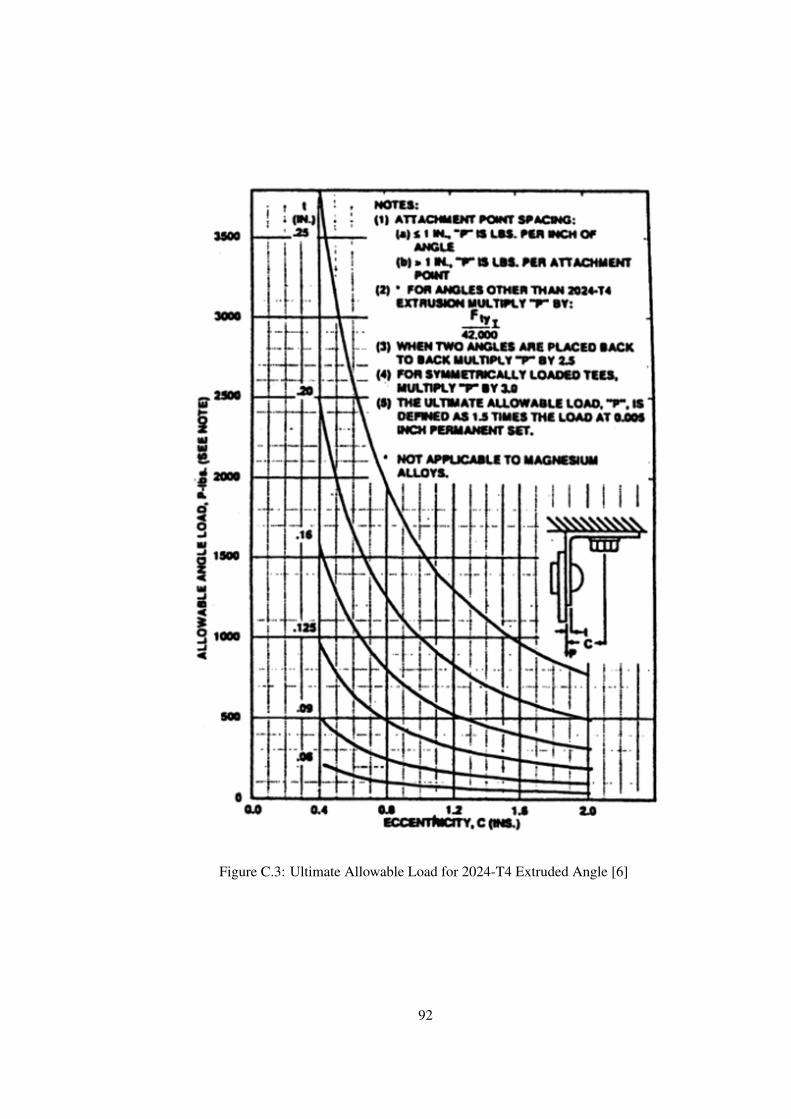
Figure C.3: Ultimate Allowable Load for 2024-T4 Extruded Angle [6]

92

C.2 Graphics presented by Niu

Figure C.4: Strength of Extruded Angle Clips (AL 2024) [7]

93

Figure C.5: Formed Sheet Angle Clips (AL 2024 and 7075) [7]

94

Figure C.6: Strength of Extruded T Clips (AL 7075) [7]

95

C.3 Graphics of ESDU 84039

Figure C.7: Maximum Bending Moment in Thin Flanges [22]

96

Figure C.8: Bending Moments in Double Sided Angles [22]

97

APPENDIX D

MATERIAL PROPERTIES and BOLT SPECIFICATIONS

D.1 AISI300MMPDS-03

1 October 2006

2-224

Table 2.7.1.0(b). Design Mechanical and Physical Properties of AISI 301andRelateda,b,c,d Stainless Steels

Specification . . . . . . AMS 5901 AMS 5517 AMS 5518 AMS 5902 AMS 5519Form . . . . . . . . . . . . Sheet and stripCondition . . . . . . . . . Annealede ¼ Hard ½ Hard ¾ Hard Full HardThickness, in. . . . . . . 0.187 ... ... ... ...Basis . . . . . . . . . . . . . S A B A B A B A BMechanical Properties:

Ftu, ksi:L . . . . . . . . . . . . . .LT . . . . . . . . . . . .

Fty, ksi:L . . . . . . . . . . . . . .LT . . . . . . . . . . . .

Fcy, ksi:L . . . . . . . . . . . . . .LT . . . . . . . . . . . .

Fsu, ksi . . . . . . . . . .Fbru, ksi:

(e/D = 1.5) . . . . .(e/D = 2.0) . . . . .

Fbry, ksi:(e/D = 1.5) . . . . .(e/D = 2.0) . . . . .

e, percent (S basis):LT . . . . . . . . . . . .

73 75

26 30

23 29 50

...162

... 55

40

124122

69 67

44 71 66

...262

...123

25

129127

83 82

54 88 69

...273

...149

...

141142

93 92

61100 77

...292

...167

f

151152

110105

69116 82

...310

...189

...

157163

118113

75127 88

...327

...202

f

168173

135133

88152 93

...342

...234

...

174175

137125

83142 95

...346

...222

f

185186

153142

94164100

...361

...249

...E, 103 ksi:

L . . . . . . . . . . . . .LT . . . . . . . . . . . .

Ec, 103 ksi:L . . . . . . . . . . . . .LT . . . . . . . . . . . .

G, 103 ksi . . . . . . . .µ . . . . . . . . . . . . . .

29.029.0

28.028.011.2

0.27

27.028.0

26.027.010.6

0.27

26.028.0

26.027.010.5

0.27

26.028.0

26.027.010.5

0.27

26.028.0

26.027.010.5

0.27Physical Properties:

, lb/in.3 . . . . . . . .C, K, and . . . . . .

0.286See Figure 2.7.1.0

a Properties also applicable to AISI 302 for the following: AMS 5516 for annealed condition, AMS 5903 for 1/4Hcondition, AMS 5904 for 1/2H condition, AMS 5905 for 3/4H condition, and AMS 5906 for full-hard condition.

b Properties also applicable to AISI 304 for the following: AMS 5513 for annealed condition, AMS 5910 for 1/4Hcondition, AMS 5911 for 1/2H condition, AMS 5912 for 3/4H condition, and AMS 5913 for full hard condition.

c Properties also applicable to AISI 316 for the following: AMS 5524 for annealed condition and AMS 5907 for 1/4Hcondition.

d Properties also applicable to AISI 303 per ASTM A 582, AISI 321 per AMS 5510, and AISI 347 per AMS 5512.e Properties for annealed (solution heat treated) condition also applicable to AISI 301 plate and to AISI 302, 303,

304, 321, and 347 sheet, strip, and plate, supplied to industry specifications.f See Table 2.7.1.0(c).

Note: Yield strength, particularly in compression, and modulus of elasticity in the longitudinal direction may be raisedappreciably by thermal stress-relieving treatment in the range 500 to 800 F.

Figure D.1: Design Mechanical and Physical Properties of AISI 301 and Relateda,b,c,d Stain-less Steels [32]

98

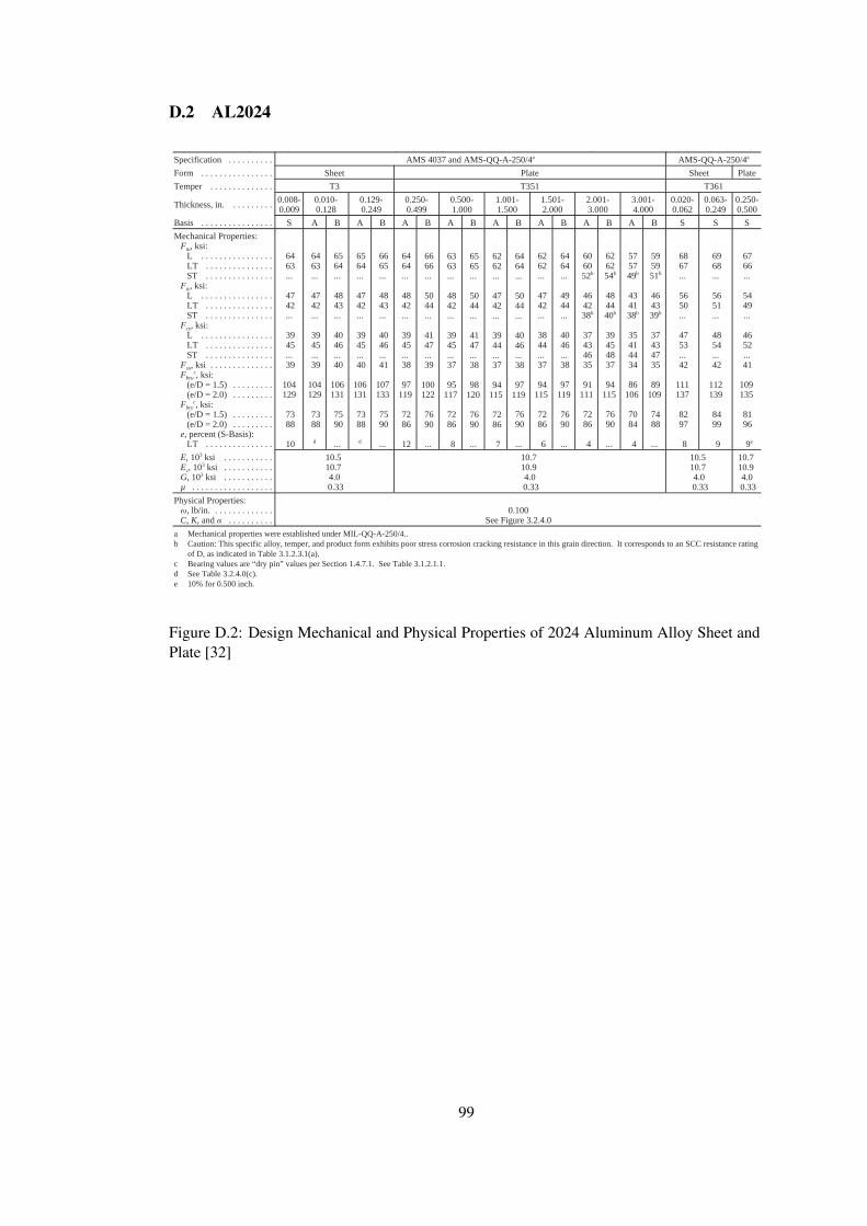
D.2 AL2024

MM

PDS-03

1 October 2006

3-86

Table 3.2.4.0(b1). Design Mechanical and Physical Properties of 2024 Aluminum Alloy Sheet and PlateSpecification . . . . . . . . . . AMS 4037 and AMS-QQ-A-250/4a AMS-QQ-A-250/4a

Form . . . . . . . . . . . . . . . . Sheet Plate Sheet PlateTemper . . . . . . . . . . . . . . T3 T351 T361

Thickness, in. . . . . . . . . . 0.008-0.009

0.010-0.128

0.129-0.249

0.250-0.499

0.500-1.000

1.001-1.500

1.501-2.000

2.001-3.000

3.001-4.000

0.020-0.062

0.063-0.249

0.250-0.500

Basis . . . . . . . . . . . . . . . . S A B A B A B A B A B A B A B A B S S SMechanical Properties:

Ftu, ksi:L . . . . . . . . . . . . . . . .LT . . . . . . . . . . . . . . .ST . . . . . . . . . . . . . . .

Fty, ksi:L . . . . . . . . . . . . . . . .LT . . . . . . . . . . . . . . .ST . . . . . . . . . . . . . . .

Fcy, ksi:L . . . . . . . . . . . . . . . .LT . . . . . . . . . . . . . . .ST . . . . . . . . . . . . . . .

Fsu, ksi . . . . . . . . . . . . . .Fbru

c, ksi:(e/D = 1.5) . . . . . . . . .(e/D = 2.0) . . . . . . . . .

Fbryc, ksi:

(e/D = 1.5) . . . . . . . . .(e/D = 2.0) . . . . . . . . .

e, percent (S-Basis):LT . . . . . . . . . . . . . . .

64 63...

47 42...

39 45... 39

104129

73 88

10

64 63...

47 42...

39 45... 39

104129

73 88

d

65 64...

48 43...

40 46... 40

106131

75 90

...

65 64...

47 42...

39 45... 40

106131

73 88

d

66 65...

48 43...

40 46... 41

107133

75 90

...

64 64...

48 42...

39 45... 38

97119

72 86

12

66 66...

50 44...

41 47... 39

100122

76 90

...

63 63...

48 42...

39 45... 37

95117

72 86

8

65 65...

50 44...

41 47... 38

98120

76 90

...

62 62...

47 42...

39 44... 37

94115

72 86

7

64 64...

50 44...

40 46... 38

97119

76 90

...

62 62...

47 42...

38 44... 37

94115

72 86

6

64 64...

49 44...

40 46... 38

97119

76 90

...

60 60 52b

46 42 38b

37 43 46 35

91111

72 86

4

62 62 54b

48 44 40b

39 45 48 37

94115

76 90

...

57 57 49b

43 41 38b

35 41 44 34

86106

70 84

4

59 59 51b

46 43 39b

37 43 47 35

89109

74 88

...

68 67...

56 50...

47 53... 42

111137

82 97

8

69 68...

56 51...

48 54... 42

112139

84 99

9

67 66...

54 49...

46 52...

41

109135

81 96

9e

E, 103 ksi . . . . . . . . . . .Ec, 103 ksi . . . . . . . . . . .G, 103 ksi . . . . . . . . . . .µ . . . . . . . . . . . . . . . . . .

10.510.7 4.0 0.33

10.710.9 4.0 0.33

10.510.7 4.0 0.33

10.710.9 4.0 0.33

Physical Properties:, lb/in. . . . . . . . . . . . . .

C, K, and . . . . . . . . . .0.100

See Figure 3.2.4.0a Mechanical properties were established under MIL-QQ-A-250/4..b Caution: This specific alloy, temper, and product form exhibits poor stress corrosion cracking resistance in this grain direction. It corresponds to an SCC resistance rating

of D, as indicated in Table 3.1.2.3.1(a).c Bearing values are “dry pin” values per Section 1.4.7.1. See Table 3.1.2.1.1.d See Table 3.2.4.0(c).e 10% for 0.500 inch.

Figure D.2: Design Mechanical and Physical Properties of 2024 Aluminum Alloy Sheet andPlate [32]

99

D.3 NAS609

Figure D.3: Bolt Dimensions and Sectional View of Standard NAS609 Series [29]

Figure D.4: Bolt Dimensions of Standard NAS609 Series [29]

100

APPENDIX E

SIMULATION MODELS PREPARED by PARAMETRIC

STUDY and COMPLETE RESULTS

E.1 Code Generated for the Description Models

LP 6 5 4 3

t/D

a/D

b/D

D

CASE

Figure E.1: Code Generated for the Description of Models

At Figure E.1, numbers paired with t/D, a/D, b/D and D shows the row number of the actual

dimensional value or coeffient in given arrays at Table 5.1. Characters paired with CAS E

shows the properties of related case. Possible cases are L, LP, T and T P. Here L and T stands

for the shape of the section where existence of P indicates that preload is applied on the bolt.

As a result, given sample shows that model has L section, preload is applied on the bolt, bolt

diameter is 12.7mm, b/D ratio is 2.0, a/D ratio is 2.3 and t/D ratio is 0.7.

101

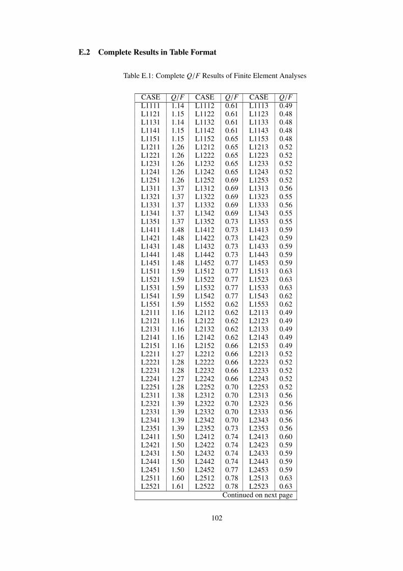
E.2 Complete Results in Table Format

Table E.1: Complete Q/F Results of Finite Element Analyses

CASE Q/F CASE Q/F CASE Q/FL1111 1.14 L1112 0.61 L1113 0.49L1121 1.15 L1122 0.61 L1123 0.48L1131 1.14 L1132 0.61 L1133 0.48L1141 1.15 L1142 0.61 L1143 0.48L1151 1.15 L1152 0.65 L1153 0.48L1211 1.26 L1212 0.65 L1213 0.52L1221 1.26 L1222 0.65 L1223 0.52L1231 1.26 L1232 0.65 L1233 0.52L1241 1.26 L1242 0.65 L1243 0.52L1251 1.26 L1252 0.69 L1253 0.52L1311 1.37 L1312 0.69 L1313 0.56L1321 1.37 L1322 0.69 L1323 0.55L1331 1.37 L1332 0.69 L1333 0.56L1341 1.37 L1342 0.69 L1343 0.55L1351 1.37 L1352 0.73 L1353 0.55L1411 1.48 L1412 0.73 L1413 0.59L1421 1.48 L1422 0.73 L1423 0.59L1431 1.48 L1432 0.73 L1433 0.59L1441 1.48 L1442 0.73 L1443 0.59L1451 1.48 L1452 0.77 L1453 0.59L1511 1.59 L1512 0.77 L1513 0.63L1521 1.59 L1522 0.77 L1523 0.63L1531 1.59 L1532 0.77 L1533 0.63L1541 1.59 L1542 0.77 L1543 0.62L1551 1.59 L1552 0.62 L1553 0.62L2111 1.16 L2112 0.62 L2113 0.49L2121 1.16 L2122 0.62 L2123 0.49L2131 1.16 L2132 0.62 L2133 0.49L2141 1.16 L2142 0.62 L2143 0.49L2151 1.16 L2152 0.66 L2153 0.49L2211 1.27 L2212 0.66 L2213 0.52L2221 1.28 L2222 0.66 L2223 0.52L2231 1.28 L2232 0.66 L2233 0.52L2241 1.27 L2242 0.66 L2243 0.52L2251 1.28 L2252 0.70 L2253 0.52L2311 1.38 L2312 0.70 L2313 0.56L2321 1.39 L2322 0.70 L2323 0.56L2331 1.39 L2332 0.70 L2333 0.56L2341 1.39 L2342 0.70 L2343 0.56L2351 1.39 L2352 0.73 L2353 0.56L2411 1.50 L2412 0.74 L2413 0.60L2421 1.50 L2422 0.74 L2423 0.59L2431 1.50 L2432 0.74 L2433 0.59L2441 1.50 L2442 0.74 L2443 0.59L2451 1.50 L2452 0.77 L2453 0.59L2511 1.60 L2512 0.78 L2513 0.63L2521 1.61 L2522 0.78 L2523 0.63

Continued on next page

102

Cont. of previous pageCASE Q/F CASE Q/F CASE Q/FL2531 1.61 L2532 0.78 L2533 0.63L2541 1.61 L2542 0.77 L2543 0.63L2551 1.61 L2552 0.63 L2553 0.63L3111 1.17 L3112 0.63 L3113 0.49L3121 1.17 L3122 0.63 L3123 0.49L3131 1.17 L3132 0.63 L3133 0.49L3141 1.17 L3142 0.63 L3143 0.49L3151 1.17 L3152 0.66 L3153 0.49L3211 1.29 L3212 0.66 L3213 0.53L3221 1.29 L3222 0.66 L3223 0.53L3231 1.29 L3232 0.66 L3233 0.53L3241 1.29 L3242 0.66 L3243 0.52L3251 1.28 L3252 0.70 L3253 0.53L3311 1.40 L3312 0.70 L3313 0.56L3321 1.40 L3322 0.70 L3323 0.56L3331 1.40 L3332 0.70 L3333 0.56L3341 1.40 L3342 0.70 L3343 0.56L3351 1.40 L3352 0.74 L3353 0.56L3411 1.51 L3412 0.74 L3413 0.60L3421 1.51 L3422 0.74 L3423 0.60L3431 1.51 L3432 0.74 L3433 0.60L3441 1.51 L3442 0.74 L3443 0.60L3451 1.51 L3452 0.78 L3453 0.60L3511 1.62 L3512 0.78 L3513 0.63L3521 1.62 L3522 0.78 L3523 0.63L3531 1.62 L3532 0.78 L3533 0.63L3541 1.62 L3542 0.78 L3543 0.63L3551 1.62 L3552 0.63 L3553 0.63L4111 1.18 L4112 0.63 L4113 0.49L4121 1.18 L4122 0.63 L4123 0.49L4131 1.18 L4132 0.63 L4133 0.49L4141 1.19 L4142 0.63 L4143 0.49L4151 1.18 L4152 0.67 L4153 0.49L4211 1.29 L4212 0.67 L4213 0.53L4221 1.30 L4222 0.67 L4223 0.53L4231 1.29 L4232 0.67 L4233 0.53L4241 1.29 L4242 0.67 L4243 0.53L4251 1.29 L4252 0.70 L4253 0.53L4311 1.40 L4312 0.70 L4313 0.56L4321 1.41 L4322 0.71 L4323 0.56L4331 1.41 L4332 0.70 L4333 0.56L4341 1.41 L4342 0.70 L4343 0.56L4351 1.41 L4352 0.74 L4353 0.56L4411 1.52 L4412 0.74 L4413 0.60L4421 1.52 L4422 0.74 L4423 0.60L4431 1.51 L4432 0.74 L4433 0.60L4441 1.52 L4442 0.74 L4443 0.60L4451 1.52 L4452 0.78 L4453 0.60L4511 1.62 L4512 0.78 L4513 0.64L4521 1.63 L4522 0.78 L4523 0.63L4531 1.63 L4532 0.78 L4533 0.63

Continued on next page

103

Cont. of previous pageCASE Q/F CASE Q/F CASE Q/FL4541 1.63 L4542 0.78 L4543 0.63L4551 1.63 L4552 0.63 L4553 0.63L5111 1.19 L5112 0.63 L5113 0.50L5121 1.19 L5122 0.63 L5123 0.49L5131 1.19 L5132 0.63 L5133 0.49L5141 1.19 L5142 0.63 L5143 0.49L5151 1.19 L5152 0.67 L5153 0.49L5211 1.30 L5212 0.67 L5213 0.53L5221 1.30 L5222 0.67 L5223 0.53L5231 1.30 L5232 0.67 L5233 0.53L5241 1.30 L5242 0.67 L5243 0.53L5251 1.30 L5252 0.71 L5253 0.53L5311 1.42 L5312 0.71 L5313 0.57L5321 1.41 L5322 0.71 L5323 0.56L5331 1.41 L5332 0.71 L5333 0.56L5341 1.41 L5342 0.71 L5343 0.56L5351 1.42 L5352 0.74 L5353 0.56L5411 1.52 L5412 0.75 L5413 0.60L5421 1.53 L5422 0.75 L5423 0.60L5431 1.52 L5432 0.75 L5433 0.60L5441 1.52 L5442 0.75 L5443 0.60L5451 1.52 L5452 0.78 L5453 0.60L5511 1.64 L5512 0.79 L5513 0.64L5521 1.64 L5522 0.78 L5523 0.64L5531 1.64 L5532 0.78 L5533 0.64L5541 1.64 L5542 0.79 L5543 0.64L5551 1.63 L5552 0.63 L5553 0.63L6111 1.19 L6112 0.63 L6113 0.50L6121 1.19 L6122 0.63 L6123 0.50L6131 1.19 L6132 0.63 L6133 0.49L6141 1.19 L6142 0.63 L6143 0.49L6151 1.19 L6152 0.67 L6153 0.49L6211 1.31 L6212 0.67 L6213 0.53L6221 1.31 L6222 0.67 L6223 0.53L6231 1.30 L6232 0.67 L6233 0.53L6241 1.30 L6242 0.67 L6243 0.53L6251 1.30 L6252 0.71 L6253 0.53L6311 1.42 L6312 0.71 L6313 0.57L6321 1.41 L6322 0.71 L6323 0.56L6331 1.42 L6332 0.71 L6333 0.56L6341 1.42 L6342 0.71 L6343 0.57L6351 1.42 L6352 0.75 L6353 0.56L6411 1.53 L6412 0.75 L6413 0.60L6421 1.53 L6422 0.75 L6423 0.60L6431 1.53 L6432 0.75 L6433 0.60L6441 1.53 L6442 0.75 L6443 0.60L6451 1.53 L6452 0.79 L6453 0.60L6511 1.63 L6512 0.79 L6513 0.64L6521 1.64 L6522 0.79 L6523 0.64L6531 1.64 L6532 0.79 L6533 0.64L6541 1.64 L6542 0.79 L6543 0.64

Continued on next page

104

Cont. of previous pageCASE Q/F CASE Q/F CASE Q/F

LP1111 1.28 LP1112 0.67 LP1113 0.52LP1121 1.28 LP1122 0.67 LP1123 0.52LP1131 1.28 LP1132 0.67 LP1133 0.52LP1141 1.28 LP1142 0.67 LP1143 0.52LP1151 1.28 LP1152 0.67 LP1153 0.52LP1211 1.40 LP1212 0.71 LP1213 0.56LP1221 1.39 LP1222 0.70 LP1223 0.55LP1231 1.39 LP1232 0.70 LP1233 0.55LP1241 1.39 LP1242 0.70 LP1243 0.55LP1251 1.39 LP1252 0.70 LP1253 0.55LP1311 1.51 LP1312 0.74 LP1313 0.59LP1321 1.50 LP1322 0.74 LP1323 0.59LP1331 1.51 LP1332 0.74 LP1333 0.59LP1341 1.51 LP1342 0.74 LP1343 0.59LP1351 1.51 LP1352 0.74 LP1353 0.59LP1411 1.62 LP1412 0.78 LP1413 0.63LP1421 1.61 LP1422 0.78 LP1423 0.63LP1431 1.62 LP1432 0.78 LP1433 0.62LP1441 1.61 LP1442 0.78 LP1443 0.63LP1451 1.62 LP1452 0.78 LP1453 0.62LP1511 1.73 LP1512 0.82 LP1513 0.66LP1521 1.72 LP1522 0.82 LP1523 0.66LP1531 1.72 LP1532 0.82 LP1533 0.66LP1541 1.72 LP1542 0.82 LP1543 0.66LP1551 1.72 LP1552 0.82 LP1553 0.66LP2111 1.28 LP2112 0.67 LP2113 0.52LP2121 1.28 LP2122 0.67 LP2123 0.52LP2131 1.28 LP2132 0.67 LP2133 0.52LP2141 1.28 LP2142 0.67 LP2143 0.52LP2151 1.28 LP2152 0.67 LP2153 0.52LP2211 1.39 LP2212 0.70 LP2213 0.55LP2221 1.39 LP2222 0.70 LP2223 0.55LP2231 1.39 LP2232 0.70 LP2233 0.55LP2241 1.39 LP2242 0.70 LP2243 0.55LP2251 1.39 LP2252 0.70 LP2253 0.55LP2311 1.50 LP2312 0.74 LP2313 0.59LP2321 1.50 LP2322 0.74 LP2323 0.59LP2331 1.51 LP2332 0.74 LP2333 0.59LP2341 1.50 LP2342 0.74 LP2343 0.59LP2351 1.50 LP2352 0.74 LP2353 0.59LP2411 1.61 LP2412 0.78 LP2413 0.63LP2421 1.61 LP2422 0.78 LP2423 0.63LP2431 1.61 LP2432 0.78 LP2433 0.62LP2441 1.61 LP2442 0.78 LP2443 0.63LP2451 1.62 LP2452 0.78 LP2453 0.63LP2511 1.72 LP2512 0.82 LP2513 0.66LP2521 1.72 LP2522 0.82 LP2523 0.66LP2531 1.72 LP2532 0.82 LP2533 0.66LP2541 1.73 LP2542 0.82 LP2543 0.66LP2551 1.72 LP2552 0.82 LP2553 0.66LP3111 1.28 LP3112 0.67 LP3113 0.52

Continued on next page

105

Cont. of previous pageCASE Q/F CASE Q/F CASE Q/F

LP3121 1.28 LP3122 0.67 LP3123 0.52LP3131 1.27 LP3132 0.67 LP3133 0.52LP3141 1.28 LP3142 0.67 LP3143 0.52LP3151 1.27 LP3152 0.67 LP3153 0.52LP3211 1.39 LP3212 0.71 LP3213 0.55LP3221 1.40 LP3222 0.71 LP3223 0.55LP3231 1.39 LP3232 0.70 LP3233 0.55LP3241 1.39 LP3242 0.71 LP3243 0.55LP3251 1.39 LP3252 0.70 LP3253 0.55LP3311 1.50 LP3312 0.74 LP3313 0.59LP3321 1.50 LP3322 0.74 LP3323 0.59LP3331 1.51 LP3332 0.74 LP3333 0.59LP3341 1.51 LP3342 0.74 LP3343 0.59LP3351 1.51 LP3352 0.74 LP3353 0.59LP3411 1.62 LP3412 0.78 LP3413 0.63LP3421 1.62 LP3422 0.78 LP3423 0.63LP3431 1.62 LP3432 0.78 LP3433 0.63LP3441 1.62 LP3442 0.78 LP3443 0.63LP3451 1.61 LP3452 0.78 LP3453 0.63LP3511 1.73 LP3512 0.82 LP3513 0.66LP3521 1.73 LP3522 0.82 LP3523 0.66LP3531 1.73 LP3532 0.82 LP3533 0.66LP3541 1.73 LP3542 0.82 LP3543 0.66LP3551 1.72 LP3552 0.82 LP3553 0.66LP4111 1.27 LP4112 0.67 LP4113 0.52LP4121 1.27 LP4122 0.67 LP4123 0.52LP4131 1.28 LP4132 0.67 LP4133 0.52LP4141 1.28 LP4142 0.67 LP4143 0.52LP4151 1.27 LP4152 0.67 LP4153 0.52LP4211 1.39 LP4212 0.70 LP4213 0.55LP4221 1.39 LP4222 0.70 LP4223 0.55LP4231 1.39 LP4232 0.70 LP4233 0.55LP4241 1.38 LP4242 0.71 LP4243 0.55LP4251 1.39 LP4252 0.70 LP4253 0.55LP4311 1.50 LP4312 0.74 LP4313 0.59LP4321 1.50 LP4322 0.74 LP4323 0.59LP4331 1.51 LP4332 0.74 LP4333 0.59LP4341 1.51 LP4342 0.74 LP4343 0.59LP4351 1.51 LP4352 0.74 LP4353 0.59LP4411 1.62 LP4412 0.78 LP4413 0.63LP4421 1.62 LP4422 0.78 LP4423 0.63LP4431 1.60 LP4432 0.78 LP4433 0.63LP4441 1.61 LP4442 0.78 LP4443 0.63LP4451 1.61 LP4452 0.78 LP4453 0.63LP4511 1.72 LP4512 0.82 LP4513 0.66LP4521 1.73 LP4522 0.82 LP4523 0.66LP4531 1.73 LP4532 0.82 LP4533 0.66LP4541 1.73 LP4542 0.82 LP4543 0.66LP4551 1.72 LP4552 0.82 LP4553 0.66LP5111 1.28 LP5112 0.67 LP5113 0.52LP5121 1.28 LP5122 0.67 LP5123 0.52

Continued on next page

106

Cont. of previous pageCASE Q/F CASE Q/F CASE Q/F

LP5131 1.28 LP5132 0.67 LP5133 0.52LP5141 1.28 LP5142 0.67 LP5143 0.52LP5151 1.28 LP5152 0.67 LP5153 0.52LP5211 1.39 LP5212 0.71 LP5213 0.56LP5221 1.39 LP5222 0.71 LP5223 0.55LP5231 1.39 LP5232 0.71 LP5233 0.55LP5241 1.39 LP5242 0.71 LP5243 0.55LP5251 1.39 LP5252 0.70 LP5253 0.55LP5311 1.51 LP5312 0.74 LP5313 0.59LP5321 1.50 LP5322 0.74 LP5323 0.59LP5331 1.51 LP5332 0.74 LP5333 0.59LP5341 1.50 LP5342 0.75 LP5343 0.59LP5351 1.51 LP5352 0.74 LP5353 0.59LP5411 1.60 LP5412 0.78 LP5413 0.63LP5421 1.62 LP5422 0.78 LP5423 0.63LP5431 1.62 LP5432 0.78 LP5433 0.63LP5441 1.62 LP5442 0.78 LP5443 0.62LP5451 1.61 LP5452 0.78 LP5453 0.63LP5511 1.73 LP5512 0.82 LP5513 0.66LP5521 1.73 LP5522 0.82 LP5523 0.66LP5531 1.73 LP5532 0.82 LP5533 0.66LP5541 1.73 LP5542 0.82 LP5543 0.66LP5551 1.72 LP5552 0.82 LP5553 0.66LP6111 1.28 LP6112 0.67 LP6113 0.52LP6121 1.28 LP6122 0.67 LP6123 0.52LP6131 1.28 LP6132 0.67 LP6133 0.52LP6141 1.28 LP6142 0.67 LP6143 0.52LP6151 1.28 LP6152 0.67 LP6153 0.52LP6211 1.39 LP6212 0.71 LP6213 0.56LP6221 1.39 LP6222 0.71 LP6223 0.55LP6231 1.39 LP6232 0.71 LP6233 0.55LP6241 1.39 LP6242 0.70 LP6243 0.55LP6251 1.39 LP6252 0.71 LP6253 0.55LP6311 1.51 LP6312 0.74 LP6313 0.59LP6321 1.50 LP6322 0.74 LP6323 0.59LP6331 1.50 LP6332 0.74 LP6333 0.59LP6341 1.50 LP6342 0.74 LP6343 0.59LP6351 1.50 LP6352 0.74 LP6353 0.59LP6411 1.61 LP6412 0.78 LP6413 0.63LP6421 1.62 LP6422 0.78 LP6423 0.62LP6431 1.61 LP6432 0.78 LP6433 0.62LP6441 1.61 LP6442 0.78 LP6443 0.62LP6451 1.61 LP6452 0.78 LP6453 0.63LP6511 1.72 LP6512 0.82 LP6513 0.66LP6521 1.72 LP6522 0.82 LP6523 0.66LP6531 1.72 LP6532 0.82 LP6533 0.66LP6541 1.72 LP6542 0.82 LP6543 0.66LP6551 1.73 LP6552 0.82 LP6553 0.66T1111 0.75 T1112 0.46 T1113 0.31T1121 0.74 T1122 0.46 T1123 0.31T1131 0.74 T1132 0.46 T1133 0.31

Continued on next page

107

Cont. of previous pageCASE Q/F CASE Q/F CASE Q/FT1141 0.74 T1142 0.46 T1143 0.31T1151 0.74 T1152 0.46 T1153 0.31T1211 0.83 T1212 0.50 T1213 0.35T1221 0.83 T1222 0.50 T1223 0.34T1231 0.83 T1232 0.50 T1233 0.34T1241 0.83 T1242 0.50 T1243 0.34T1251 0.83 T1252 0.50 T1253 0.34T1311 0.92 T1312 0.54 T1313 0.38T1321 0.92 T1322 0.54 T1323 0.38T1331 0.92 T1332 0.54 T1333 0.38T1341 0.92 T1342 0.54 T1343 0.37T1351 0.92 T1352 0.54 T1353 0.37T1411 1.01 T1412 0.59 T1413 0.42T1421 1.01 T1422 0.58 T1423 0.41T1431 1.01 T1432 0.58 T1433 0.41T1441 1.01 T1442 0.58 T1443 0.41T1451 1.00 T1452 0.58 T1453 0.41T1511 1.10 T1512 0.63 T1513 0.45T1521 1.10 T1522 0.63 T1523 0.45T1531 1.10 T1532 0.63 T1533 0.45T1541 1.10 T1542 0.63 T1543 0.44T1551 1.10 T1552 0.63 T1553 0.44T2111 0.78 T2112 0.47 T2113 0.32T2121 0.78 T2122 0.47 T2123 0.32T2131 0.78 T2132 0.47 T2133 0.31T2141 0.78 T2142 0.47 T2143 0.31T2151 0.78 T2152 0.47 T2153 0.31T2211 0.87 T2212 0.51 T2213 0.35T2221 0.87 T2222 0.51 T2223 0.35T2231 0.87 T2232 0.51 T2233 0.35T2241 0.87 T2242 0.51 T2243 0.35T2251 0.87 T2252 0.51 T2253 0.34T2311 0.95 T2312 0.55 T2313 0.38T2321 0.96 T2322 0.55 T2323 0.38T2331 0.96 T2332 0.55 T2333 0.38T2341 0.96 T2342 0.55 T2343 0.38T2351 0.95 T2352 0.55 T2353 0.38T2411 1.07 T2412 0.60 T2413 0.42T2421 1.05 T2422 0.59 T2423 0.42T2431 1.05 T2432 0.59 T2433 0.42T2441 1.05 T2442 0.59 T2443 0.41T2451 1.05 T2452 0.59 T2453 0.41T2511 1.14 T2512 0.64 T2513 0.46T2521 1.14 T2522 0.64 T2523 0.45T2531 1.14 T2532 0.64 T2533 0.45T2541 1.14 T2542 0.64 T2543 0.45T2551 1.14 T2552 0.64 T2553 0.45T3111 0.80 T3112 0.48 T3113 0.32T3121 0.80 T3122 0.48 T3123 0.32T3131 0.80 T3132 0.48 T3133 0.32T3141 0.79 T3142 0.48 T3143 0.32

Continued on next page

108

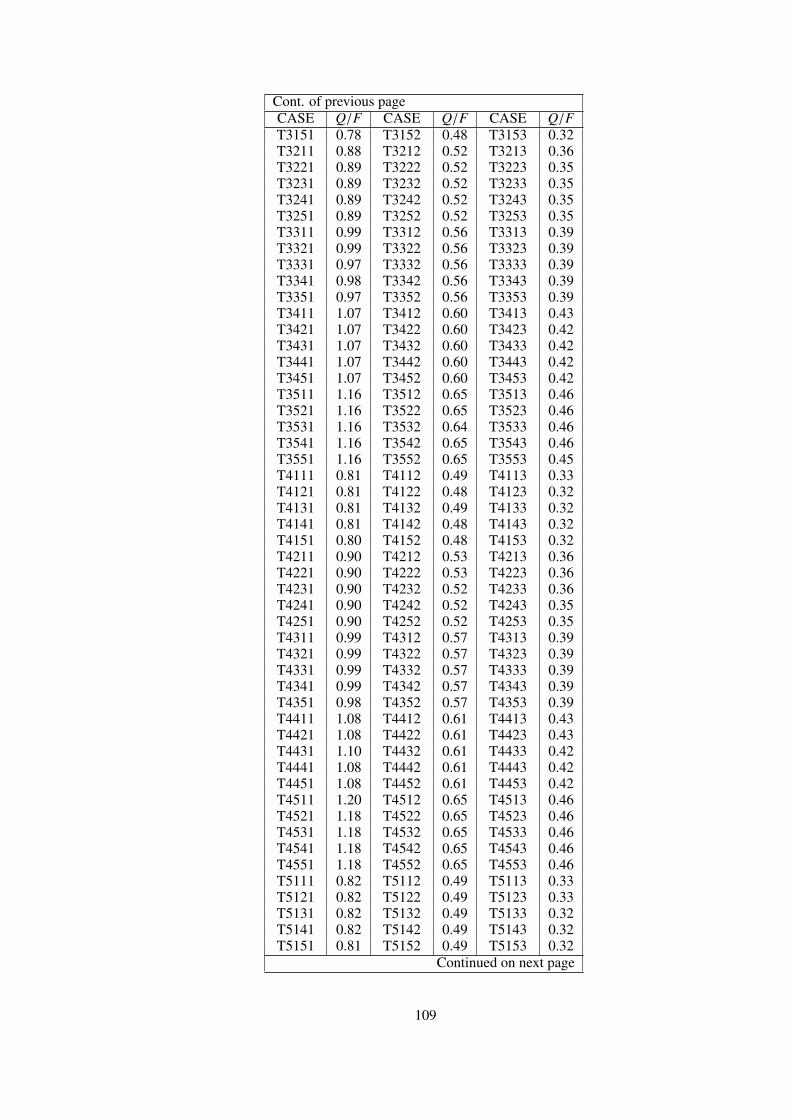
Cont. of previous pageCASE Q/F CASE Q/F CASE Q/FT3151 0.78 T3152 0.48 T3153 0.32T3211 0.88 T3212 0.52 T3213 0.36T3221 0.89 T3222 0.52 T3223 0.35T3231 0.89 T3232 0.52 T3233 0.35T3241 0.89 T3242 0.52 T3243 0.35T3251 0.89 T3252 0.52 T3253 0.35T3311 0.99 T3312 0.56 T3313 0.39T3321 0.99 T3322 0.56 T3323 0.39T3331 0.97 T3332 0.56 T3333 0.39T3341 0.98 T3342 0.56 T3343 0.39T3351 0.97 T3352 0.56 T3353 0.39T3411 1.07 T3412 0.60 T3413 0.43T3421 1.07 T3422 0.60 T3423 0.42T3431 1.07 T3432 0.60 T3433 0.42T3441 1.07 T3442 0.60 T3443 0.42T3451 1.07 T3452 0.60 T3453 0.42T3511 1.16 T3512 0.65 T3513 0.46T3521 1.16 T3522 0.65 T3523 0.46T3531 1.16 T3532 0.64 T3533 0.46T3541 1.16 T3542 0.65 T3543 0.46T3551 1.16 T3552 0.65 T3553 0.45T4111 0.81 T4112 0.49 T4113 0.33T4121 0.81 T4122 0.48 T4123 0.32T4131 0.81 T4132 0.49 T4133 0.32T4141 0.81 T4142 0.48 T4143 0.32T4151 0.80 T4152 0.48 T4153 0.32T4211 0.90 T4212 0.53 T4213 0.36T4221 0.90 T4222 0.53 T4223 0.36T4231 0.90 T4232 0.52 T4233 0.36T4241 0.90 T4242 0.52 T4243 0.35T4251 0.90 T4252 0.52 T4253 0.35T4311 0.99 T4312 0.57 T4313 0.39T4321 0.99 T4322 0.57 T4323 0.39T4331 0.99 T4332 0.57 T4333 0.39T4341 0.99 T4342 0.57 T4343 0.39T4351 0.98 T4352 0.57 T4353 0.39T4411 1.08 T4412 0.61 T4413 0.43T4421 1.08 T4422 0.61 T4423 0.43T4431 1.10 T4432 0.61 T4433 0.42T4441 1.08 T4442 0.61 T4443 0.42T4451 1.08 T4452 0.61 T4453 0.42T4511 1.20 T4512 0.65 T4513 0.46T4521 1.18 T4522 0.65 T4523 0.46T4531 1.18 T4532 0.65 T4533 0.46T4541 1.18 T4542 0.65 T4543 0.46T4551 1.18 T4552 0.65 T4553 0.46T5111 0.82 T5112 0.49 T5113 0.33T5121 0.82 T5122 0.49 T5123 0.33T5131 0.82 T5132 0.49 T5133 0.32T5141 0.82 T5142 0.49 T5143 0.32T5151 0.81 T5152 0.49 T5153 0.32

Continued on next page

109

Cont. of previous pageCASE Q/F CASE Q/F CASE Q/FT5211 0.91 T5212 0.53 T5213 0.36T5221 0.91 T5222 0.53 T5223 0.36T5231 0.91 T5232 0.53 T5233 0.36T5241 0.91 T5242 0.53 T5243 0.36T5251 0.91 T5252 0.53 T5253 0.36T5311 1.00 T5312 0.57 T5313 0.40T5321 1.00 T5322 0.57 T5323 0.39T5331 1.00 T5332 0.57 T5333 0.39T5341 1.00 T5342 0.57 T5343 0.39T5351 1.00 T5352 0.57 T5353 0.39T5411 1.09 T5412 0.61 T5413 0.43T5421 1.09 T5422 0.61 T5423 0.43T5431 1.09 T5432 0.61 T5433 0.43T5441 1.10 T5442 0.61 T5443 0.43T5451 1.09 T5452 0.61 T5453 0.43T5511 1.19 T5512 0.65 T5513 0.46T5521 1.21 T5522 0.65 T5523 0.46T5531 1.19 T5532 0.65 T5533 0.46T5541 1.19 T5542 0.65 T5543 0.46T5551 1.19 T5552 0.65 T5553 0.46T6111 0.83 T6112 0.49 T6113 0.33T6121 0.83 T6122 0.49 T6123 0.33T6131 0.83 T6132 0.49 T6133 0.33T6141 0.83 T6142 0.49 T6143 0.32T6151 0.83 T6152 0.49 T6153 0.32T6211 0.92 T6212 0.53 T6213 0.36T6221 0.92 T6222 0.53 T6223 0.36T6231 0.92 T6232 0.53 T6233 0.36T6241 0.93 T6242 0.53 T6243 0.36T6251 0.93 T6252 0.53 T6253 0.36T6311 1.01 T6312 0.57 T6313 0.40T6321 1.01 T6322 0.57 T6323 0.40T6331 1.01 T6332 0.57 T6333 0.39T6341 1.01 T6342 0.57 T6343 0.39T6351 1.01 T6352 0.57 T6353 0.39T6411 1.10 T6412 0.61 T6413 0.43T6421 1.11 T6422 0.61 T6423 0.43T6431 1.10 T6432 0.61 T6433 0.43T6441 1.10 T6442 0.61 T6443 0.43T6451 1.11 T6452 0.61 T6453 0.43T6511 1.20 T6512 0.65 T6513 0.47T6521 1.20 T6522 0.66 T6523 0.47T6531 1.20 T6532 0.66 T6533 0.46T6541 1.20 T6542 0.66 T6543 0.46T6551 1.21 T6552 0.66 T6553 0.46

TP1111 1.00 TP1112 0.56 TP1113 0.37TP1121 1.00 TP1122 0.56 TP1123 0.37TP1131 1.00 TP1132 0.56 TP1133 0.37TP1141 0.99 TP1142 0.56 TP1143 0.37TP1151 0.99 TP1152 0.56 TP1153 0.37TP1211 1.09 TP1212 0.60 TP1213 0.41

Continued on next page

110

Cont. of previous pageCASE Q/F CASE Q/F CASE Q/F

TP1221 1.09 TP1222 0.60 TP1223 0.41TP1231 1.09 TP1232 0.60 TP1233 0.40TP1241 1.09 TP1242 0.60 TP1243 0.40TP1251 1.09 TP1252 0.60 TP1253 0.40TP1311 1.19 TP1312 0.64 TP1313 0.44TP1321 1.19 TP1322 0.64 TP1323 0.44TP1331 1.19 TP1332 0.64 TP1333 0.44TP1341 1.19 TP1342 0.64 TP1343 0.44TP1351 1.19 TP1352 0.64 TP1353 0.44TP1411 1.29 TP1412 0.68 TP1413 0.48TP1421 1.29 TP1422 0.68 TP1423 0.48TP1431 1.29 TP1432 0.68 TP1433 0.47TP1441 1.29 TP1442 0.68 TP1443 0.47TP1451 1.29 TP1452 0.68 TP1453 0.47TP1511 1.39 TP1512 0.73 TP1513 0.51TP1521 1.39 TP1522 0.72 TP1523 0.51TP1531 1.39 TP1532 0.72 TP1533 0.51TP1541 1.39 TP1542 0.73 TP1543 0.51TP1551 1.39 TP1552 0.72 TP1553 0.51TP2111 1.00 TP2112 0.56 TP2113 0.37TP2121 1.00 TP2122 0.56 TP2123 0.37TP2131 1.00 TP2132 0.56 TP2133 0.37TP2141 1.00 TP2142 0.56 TP2143 0.37TP2151 1.00 TP2152 0.56 TP2153 0.37TP2211 1.09 TP2212 0.60 TP2213 0.41TP2221 1.09 TP2222 0.60 TP2223 0.41TP2231 1.09 TP2232 0.60 TP2233 0.40TP2241 1.09 TP2242 0.60 TP2243 0.40TP2251 1.10 TP2252 0.60 TP2253 0.40TP2311 1.19 TP2312 0.64 TP2313 0.44TP2321 1.20 TP2322 0.64 TP2323 0.44TP2331 1.20 TP2332 0.64 TP2333 0.44TP2341 1.20 TP2342 0.64 TP2343 0.44TP2351 1.20 TP2352 0.64 TP2353 0.44TP2411 1.31 TP2412 0.68 TP2413 0.48TP2421 1.29 TP2422 0.68 TP2423 0.48TP2431 1.29 TP2432 0.68 TP2433 0.47TP2441 1.29 TP2442 0.68 TP2443 0.47TP2451 1.29 TP2452 0.68 TP2453 0.47TP2511 1.39 TP2512 0.73 TP2513 0.51TP2521 1.39 TP2522 0.73 TP2523 0.51TP2531 1.39 TP2532 0.72 TP2533 0.51TP2541 1.39 TP2542 0.72 TP2543 0.51TP2551 1.39 TP2552 0.72 TP2553 0.51TP3111 1.00 TP3112 0.56 TP3113 0.37TP3121 1.00 TP3122 0.56 TP3123 0.37TP3131 1.00 TP3132 0.56 TP3133 0.37TP3141 1.00 TP3142 0.56 TP3143 0.37TP3151 1.00 TP3152 0.56 TP3153 0.37TP3211 1.09 TP3212 0.60 TP3213 0.41TP3221 1.09 TP3222 0.60 TP3223 0.41

Continued on next page

111

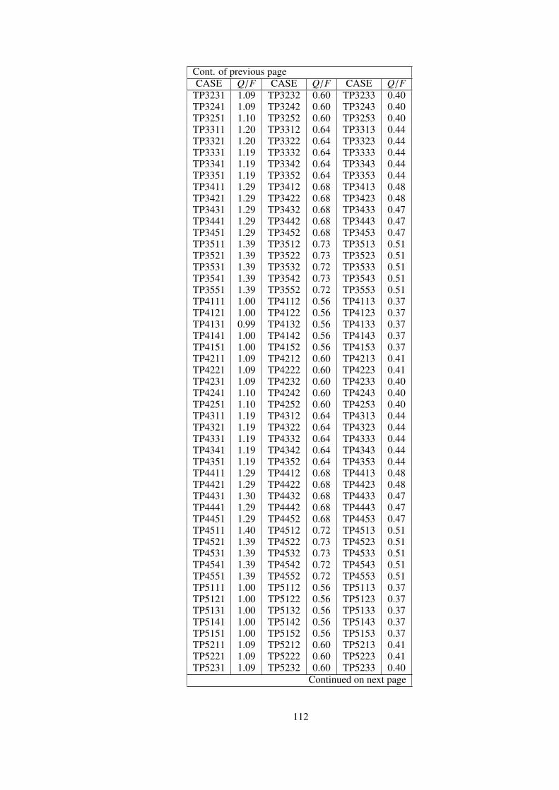
Cont. of previous pageCASE Q/F CASE Q/F CASE Q/F

TP3231 1.09 TP3232 0.60 TP3233 0.40TP3241 1.09 TP3242 0.60 TP3243 0.40TP3251 1.10 TP3252 0.60 TP3253 0.40TP3311 1.20 TP3312 0.64 TP3313 0.44TP3321 1.20 TP3322 0.64 TP3323 0.44TP3331 1.19 TP3332 0.64 TP3333 0.44TP3341 1.19 TP3342 0.64 TP3343 0.44TP3351 1.19 TP3352 0.64 TP3353 0.44TP3411 1.29 TP3412 0.68 TP3413 0.48TP3421 1.29 TP3422 0.68 TP3423 0.48TP3431 1.29 TP3432 0.68 TP3433 0.47TP3441 1.29 TP3442 0.68 TP3443 0.47TP3451 1.29 TP3452 0.68 TP3453 0.47TP3511 1.39 TP3512 0.73 TP3513 0.51TP3521 1.39 TP3522 0.73 TP3523 0.51TP3531 1.39 TP3532 0.72 TP3533 0.51TP3541 1.39 TP3542 0.73 TP3543 0.51TP3551 1.39 TP3552 0.72 TP3553 0.51TP4111 1.00 TP4112 0.56 TP4113 0.37TP4121 1.00 TP4122 0.56 TP4123 0.37TP4131 0.99 TP4132 0.56 TP4133 0.37TP4141 1.00 TP4142 0.56 TP4143 0.37TP4151 1.00 TP4152 0.56 TP4153 0.37TP4211 1.09 TP4212 0.60 TP4213 0.41TP4221 1.09 TP4222 0.60 TP4223 0.41TP4231 1.09 TP4232 0.60 TP4233 0.40TP4241 1.10 TP4242 0.60 TP4243 0.40TP4251 1.10 TP4252 0.60 TP4253 0.40TP4311 1.19 TP4312 0.64 TP4313 0.44TP4321 1.19 TP4322 0.64 TP4323 0.44TP4331 1.19 TP4332 0.64 TP4333 0.44TP4341 1.19 TP4342 0.64 TP4343 0.44TP4351 1.19 TP4352 0.64 TP4353 0.44TP4411 1.29 TP4412 0.68 TP4413 0.48TP4421 1.29 TP4422 0.68 TP4423 0.48TP4431 1.30 TP4432 0.68 TP4433 0.47TP4441 1.29 TP4442 0.68 TP4443 0.47TP4451 1.29 TP4452 0.68 TP4453 0.47TP4511 1.40 TP4512 0.72 TP4513 0.51TP4521 1.39 TP4522 0.73 TP4523 0.51TP4531 1.39 TP4532 0.73 TP4533 0.51TP4541 1.39 TP4542 0.72 TP4543 0.51TP4551 1.39 TP4552 0.72 TP4553 0.51TP5111 1.00 TP5112 0.56 TP5113 0.37TP5121 1.00 TP5122 0.56 TP5123 0.37TP5131 1.00 TP5132 0.56 TP5133 0.37TP5141 1.00 TP5142 0.56 TP5143 0.37TP5151 1.00 TP5152 0.56 TP5153 0.37TP5211 1.09 TP5212 0.60 TP5213 0.41TP5221 1.09 TP5222 0.60 TP5223 0.41TP5231 1.09 TP5232 0.60 TP5233 0.40

Continued on next page

112

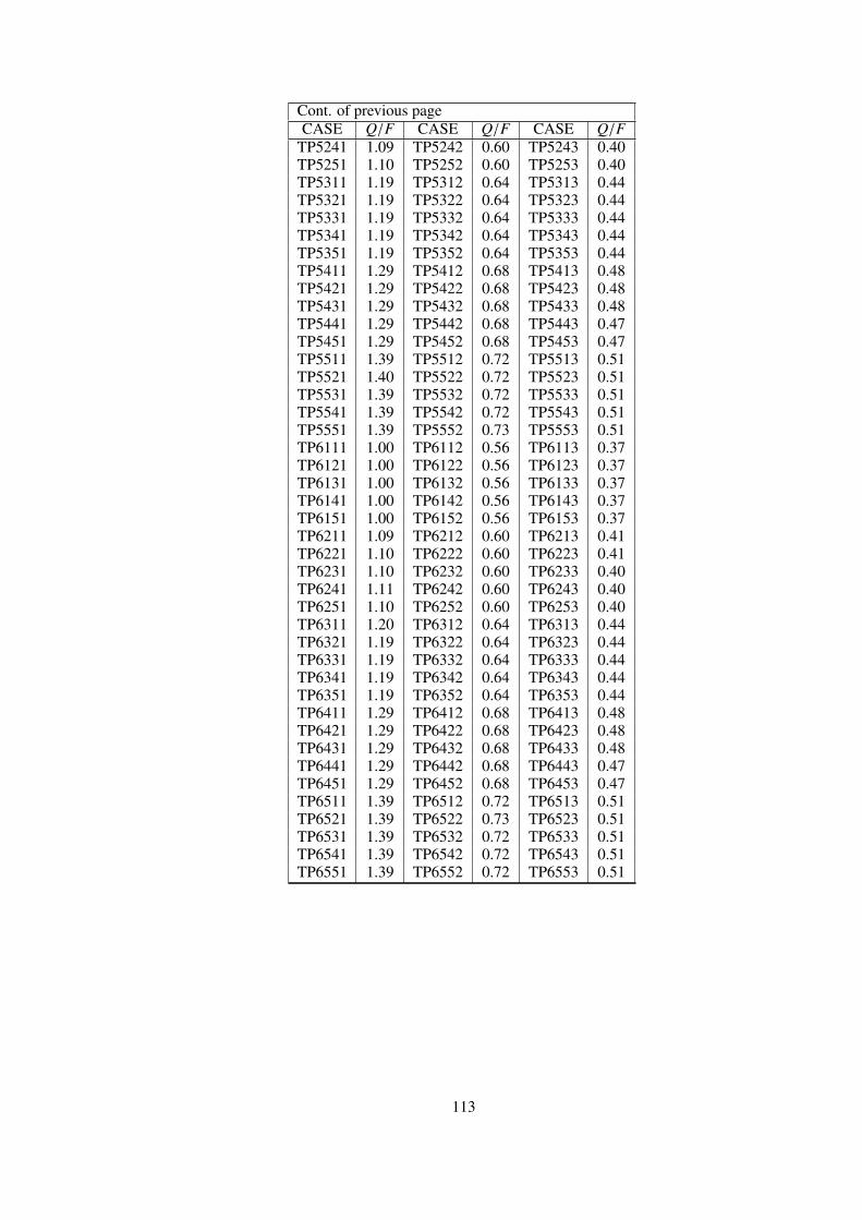
Cont. of previous pageCASE Q/F CASE Q/F CASE Q/F

TP5241 1.09 TP5242 0.60 TP5243 0.40TP5251 1.10 TP5252 0.60 TP5253 0.40TP5311 1.19 TP5312 0.64 TP5313 0.44TP5321 1.19 TP5322 0.64 TP5323 0.44TP5331 1.19 TP5332 0.64 TP5333 0.44TP5341 1.19 TP5342 0.64 TP5343 0.44TP5351 1.19 TP5352 0.64 TP5353 0.44TP5411 1.29 TP5412 0.68 TP5413 0.48TP5421 1.29 TP5422 0.68 TP5423 0.48TP5431 1.29 TP5432 0.68 TP5433 0.48TP5441 1.29 TP5442 0.68 TP5443 0.47TP5451 1.29 TP5452 0.68 TP5453 0.47TP5511 1.39 TP5512 0.72 TP5513 0.51TP5521 1.40 TP5522 0.72 TP5523 0.51TP5531 1.39 TP5532 0.72 TP5533 0.51TP5541 1.39 TP5542 0.72 TP5543 0.51TP5551 1.39 TP5552 0.73 TP5553 0.51TP6111 1.00 TP6112 0.56 TP6113 0.37TP6121 1.00 TP6122 0.56 TP6123 0.37TP6131 1.00 TP6132 0.56 TP6133 0.37TP6141 1.00 TP6142 0.56 TP6143 0.37TP6151 1.00 TP6152 0.56 TP6153 0.37TP6211 1.09 TP6212 0.60 TP6213 0.41TP6221 1.10 TP6222 0.60 TP6223 0.41TP6231 1.10 TP6232 0.60 TP6233 0.40TP6241 1.11 TP6242 0.60 TP6243 0.40TP6251 1.10 TP6252 0.60 TP6253 0.40TP6311 1.20 TP6312 0.64 TP6313 0.44TP6321 1.19 TP6322 0.64 TP6323 0.44TP6331 1.19 TP6332 0.64 TP6333 0.44TP6341 1.19 TP6342 0.64 TP6343 0.44TP6351 1.19 TP6352 0.64 TP6353 0.44TP6411 1.29 TP6412 0.68 TP6413 0.48TP6421 1.29 TP6422 0.68 TP6423 0.48TP6431 1.29 TP6432 0.68 TP6433 0.48TP6441 1.29 TP6442 0.68 TP6443 0.47TP6451 1.29 TP6452 0.68 TP6453 0.47TP6511 1.39 TP6512 0.72 TP6513 0.51TP6521 1.39 TP6522 0.73 TP6523 0.51TP6531 1.39 TP6532 0.72 TP6533 0.51TP6541 1.39 TP6542 0.72 TP6543 0.51TP6551 1.39 TP6552 0.72 TP6553 0.51

113

APPENDIX F

MEDIAL AXES MESHING ALGORITHM

Properties and benefits of medial axes meshing technique can be read through Abaqus docu-

mentation [27]. Benefits of the technique are tried to be illustrated with examples in Figure F.1

and F.2. Figures at right hand side are showing the meshes obtained by medial axes meshing

algorithm.

Figure F.1: Clip Flange Mesh Choices

Figure F.2: Bolt Mesh Choices

114