1

Data Appendix to “Economic Growth in the Information Age”

Dale W. Jorgenson, Mun Ho, Ankur Patel, and Jon Samuels

Draft April 27 2014

A. Introduction and Classifications

A.1 Labor input by NAICS industries

A.1.1 Methodology

A.1.2 Current Population Survey in NAICS [2003-2010]

A.1.3 Converting SIC labor matrices [DJA88, 1960-2002]

A.1.4 Converting SIC labor matrices [DJA67, 1947-60]

A.1.5 Linking the CPS SIC in 2002 with NAICS in 2003

A.1.6 Linking NAICS series [1947-2010]

A.1.7 Results

A.2 Capital input by NAICS industries

A.2.1 Methodology

A.2.2 Investment and stock data by industry

A.2.3 Value added and value of capital input

A.2.4 Results

A.3 Intermediate input

A.3.1 Nominal input-output tables

A.3.2 Industry and commodity prices

A.3.3 Import prices

A.3.4 Supply Prices

2

3

A. Introduction and Classifications

We begin with a brief reminder of the recent history of industry level accounts in the U.S.

The NAICS was adopted in 1997 to replace the Standard Industrial Classification (SIC) system; the

SIC was the basis on the industry productivity measures in Jorgenson, Gollop and Fraumeni (1987),

Jorgenson, Ho and Stiroh (2005) and Jorgenson, Ho, Samuels and Stiroh (2007). The first version of

GDP by industry in NAICS in the National Accounts (NIPA) was released in March 2004 with data

covering 1998-2002 for 65 industries. In that version of the NIPA, the data for 1948-86 was in the

SIC(1972) system and in SIC(1987) for the 1987-2000 data. The BEA also provides gross output

estimates for a more detailed set of industries but “does not include these detailed estimates in the

published tables because their quality is significantly less than that of the higher-level aggregates in

which they are included.” For these unpublished tables, output data is provided for 426 industries (in

NAICS-2002).

These early versions of the NAICS data for 1998 -2007 were used in Jorgenson, Ho and

Samuels (2011) to generate a time series in NAICS for 1960-2007 by linking to the earlier SIC based

input-output data used in Jorgenson, Ho, Samuels, Stiroh (2007). These will be referred to as

JHS(2011) and JHSS(2007) below.

In the more recent release in December 2011, the BEA provided GDP-by-Industry estimates

for 65 industries (in NAICS2002) back to 1977, and for 22 industry groups for the earlier period

1947-1976. These 65 industries are the same as those reported in the NIPAs in 2011. The estimates

for 1987-2000 are described in Yuskavage and Pho (2004), and for 1947-86 in Yuskavage and Fahim-

Nader (2005). The important innovation by the BEA was the estimation of a times series of Use and

Make tables back to 1947 on a consistent NAICS classification. This series of tables covered the

same 65 industries for 1963-1997, and for the 1947-62 period, they covered 46 industries. These were

made by Mark Planting as a special assignment from the BEA.

We made use of these two main BEA series – the 1947-97 IO tables in NAICS estimated by

Planting, and the annual IO tables for 1998-2010 from the BEA Industry Division – to estimate the

inter-industry transactions and the value added for our industries. We also supplemented these data

with information from the Bureau of Labor Statistics (BLS) and other sources.

The data for labor and capital accumulation was also changed over to NAICS during this

period. There is unfortunately, no parallel official effort to convert the historical labor data from SIC

to NAICS. The BEA investment data in the Fixed Asset Accounts provides an estimate of historical

4

investment by asset type in NAICS. As with the output accounts, these detailed investment data are

not in the official publications “because they are less reliable than the higher level aggregates in

which they are included.”

The three sections of the rest of this appendix describes how we estimated the labor input,

capital input and intermediate input for each industry from these primary data. We focus here on how

we converted SIC based data into NAICS, the general methodology is given in JHS (2005).

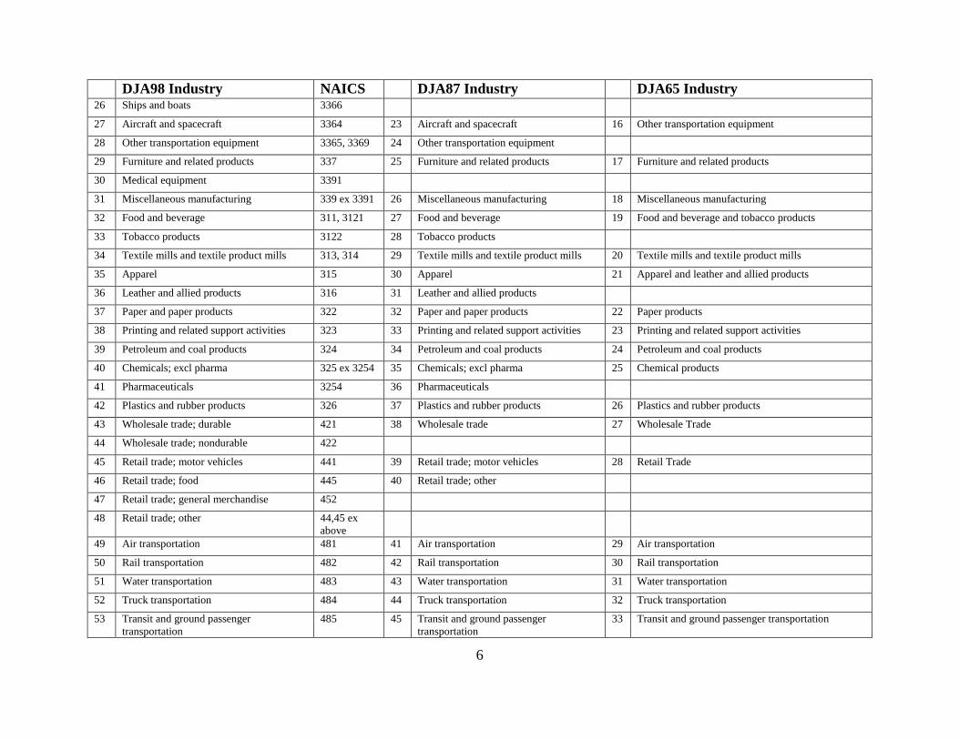
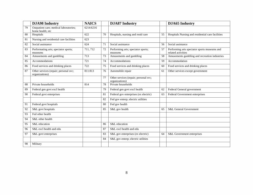
We construct data for various sets of industries, each set designed to fulfill the aims of a

particular study. At the most detailed level we identify 98 NAICS industries as listed in Table A1 in

the column marked “DJA98”. We then aggregate these to two other smaller sets of industries; BEA65

correspond to the industries in the BEA’s time series of input-output accounts while DJA87 are the

industries used in Jorgenson, Ho and Samuels (2013) with more detail on the Information Technology

sectors.

5

Table A1. Industry classifications

DJA98 Industry NAICS DJA87 Industry DJA65 Industry 1 Farms 111, 112 1 Farms 1 Farms

2 Forestry and related activities 113:115 ex

1141

2 Forestry and related activities 2 Forestry fishing and related activities

3 Fishing 1141

4 Oil and gas extraction 211 3 Oil and gas extraction 3 Oil and gas extraction

5 Coal mining 2121 4 Coal mining 4 Mining except oil and gas

6 Non-energy mining 2122, 2123 5 Non-energy mining

7 Support activities for mining 2130 6 Support activities for mining 5 Support activities for mining

8 Electric power: generation; transmission;

distribution

2211 7 Electric power: generation; transmission;

distribution

6 Utilities

9 Natural gas distribution 2212 8 Natural gas distribution

10 Water and sewage 2213 9 Water and sewage

11 Construction 230 10 Construction 7 Construction

12 Wood products 11 Wood products 8 Wood products

13 Nonmetallic mineral products 327 12 Nonmetallic mineral products 9 Nonmetallic mineral products

14 Primary metals; iron and steel 3311, 3312 13 Primary metals; iron and steel 10 Primary metals

15 Primary metals; non-ferrous metals 3313:3315 14 Primary metals; non-ferrous metals

16 Fabricated metal products 332 15 Fabricated metal products 11 Fabricated metal products

17 Machinery 333 16 Machinery 12 Machinery

18 Computer and electronic products 3341 17 Computer and peripheral equip mfg 13 Computer and electronic products

19 Telecommunication equipment 3342 18 Communications equipment mfg

20 Radio and TV receivers 3343, 3346

21 Electronic components and products 3344 19 Semiconductor and other Electronic

component mfg

22 Instruments 3345 20 Other electronic equipment

23 Insulated wire 33592

24 Other electrical machinery 335 ex

33592

21 Electrical equipment 14 Electrical equipment appliances and components

25 Motor vehicles and parts 3361:3363 22 Motor vehicles and parts 15 Motor vehicles bodies and trailers and parts

6

DJA98 Industry NAICS DJA87 Industry DJA65 Industry 26 Ships and boats 3366

27 Aircraft and spacecraft 3364 23 Aircraft and spacecraft 16 Other transportation equipment

28 Other transportation equipment 3365, 3369 24 Other transportation equipment

29 Furniture and related products 337 25 Furniture and related products 17 Furniture and related products

30 Medical equipment 3391

31 Miscellaneous manufacturing 339 ex 3391 26 Miscellaneous manufacturing 18 Miscellaneous manufacturing

32 Food and beverage 311, 3121 27 Food and beverage 19 Food and beverage and tobacco products

33 Tobacco products 3122 28 Tobacco products

34 Textile mills and textile product mills 313, 314 29 Textile mills and textile product mills 20 Textile mills and textile product mills

35 Apparel 315 30 Apparel 21 Apparel and leather and allied products

36 Leather and allied products 316 31 Leather and allied products

37 Paper and paper products 322 32 Paper and paper products 22 Paper products

38 Printing and related support activities 323 33 Printing and related support activities 23 Printing and related support activities

39 Petroleum and coal products 324 34 Petroleum and coal products 24 Petroleum and coal products

40 Chemicals; excl pharma 325 ex 3254 35 Chemicals; excl pharma 25 Chemical products

41 Pharmaceuticals 3254 36 Pharmaceuticals

42 Plastics and rubber products 326 37 Plastics and rubber products 26 Plastics and rubber products

43 Wholesale trade; durable 421 38 Wholesale trade 27 Wholesale Trade

44 Wholesale trade; nondurable 422

45 Retail trade; motor vehicles 441 39 Retail trade; motor vehicles 28 Retail Trade

46 Retail trade; food 445 40 Retail trade; other

47 Retail trade; general merchandise 452

48 Retail trade; other 44,45 ex

above

49 Air transportation 481 41 Air transportation 29 Air transportation

50 Rail transportation 482 42 Rail transportation 30 Rail transportation

51 Water transportation 483 43 Water transportation 31 Water transportation

52 Truck transportation 484 44 Truck transportation 32 Truck transportation

53 Transit and ground passenger

transportation

485 45 Transit and ground passenger

transportation

33 Transit and ground passenger transportation

7

DJA98 Industry NAICS DJA87 Industry DJA65 Industry 54 Pipelines 486 46 Pipelines 34 Pipeline transportation

55 Other transportation and support activities 487:492 47 Other transportation and support

activities

35 Other transportation and support activities

56 Warehousing and storage 493 48 Warehousing and storage 36 Warehousing and storage

57 Newspaper; periodical; book publishers 5111 49 Newspaper; periodical; book publishers 37 Publishing industries (includes software)

58 Software publishing 5112 50 Software publishing

59 Motion picture and sound recording

industries

512 51 Motion picture and sound recording

industries

38 Motion picture and sound recording industries

60 Radio; TV; cable 515 52 Broadcasting 39 Broadcasting and telecommunications

61 Telecommunications 517 53 Telecommunications

62 Information and data processing services 516, 518,519 54 Information and data processing services 40 Information and data processing services

63 Federal reserve banks; credit

intermediation

521, 522 55 Federal reserve banks; credit

intermediation

41 Federal Reserve banks credit intermediation and

related activities

64 Securities; commodity contracts;

investments

523 56 Securities; commodity contracts;

investments

42 Securities commodity contracts and investments

65 Insurance carriers and related activities 524 57 Insurance carriers and related activities 43 Insurance carriers and related activities

66 Funds and trusts 525 58 Funds and trusts 44 Funds trusts and other financial vehicles

67 Real estate (rental) 531 59 Real Estate + OOH (intermediate only) 45 Real estate

68 Real estate (owner occupied) ooh 60 OOH (VA only)

69 Rental and leasing services; lessors of

intangibles

532:533 61 Rental and leasing services; lessors of

intangibles

46 Rental and leasing services and lessors of intangible

assets

70 Legal services 5411 62 Legal services 47 Legal services

71 Computer systems design and related

services

5415 63 Computer systems design and related

services

48 Computer systems design and related services

72 Misc. professional; scientific; and

technical services

541* ex

1,5,7

64 Misc. professional, scientific 49 Miscellaneous professional scientific and technical

services

73 Scientific research and development;

other prof.

5417

74 Management of companies and

enterprises

55 65 Management of companies and

enterprises

50 Management of companies and enterprises

75 Administrative & support services 561 66 Administrative & support services 51 Administrative and support services

76 Waste management 562 67 Waste management 52 Waste management and remediation services

77 Educational services 61 68 Educational services 53 Educational services

78 Offices of physicians; dentists; other

practitioners

6211:6213 69 Ambulatory health care services 54 Ambulatory health care services

8

DJA98 Industry NAICS DJA87 Industry DJA65 Industry 79 Outpatient care; medical laboratories;

home health; etc

6214:6216

80 Hospitals 622 70 Hospitals, nursing and resid care 55 Hospitals Nursing and residential care facilities

81 Nursing and residential care facilities 623

82 Social assistance 624 71 Social assistance 56 Social assistance

83 Performating arts; spectator sports;

museums

711, 712 72 Performing arts; spectator sports;

museums

57 Performing arts spectator sports museums and

related activities

84 Amusements and gambling 713 73 Amusements and gambling 58 Amusements gambling and recreation industries

85 Accommodations 721 74 Accommodations 59 Accommodation

86 Food services and drinking places 722 75 Food services and drinking places 60 Food services and drinking places

87 Other services (repair; personal svc;

organizations)

811:813 76 Automobile repair 61 Other services except government

77 Other services (repair; personal svc;

organizations)

88 Private households 814 78 Private households

89 Federal gen govt excl health 79 Federal gen govt excl health 62 Federal General government

90 Federal govt enterprises 81 Federal gov enterprises (ex electric) 63 Federal Government enterprises

82 Fed gov enterp; electric utilities

91 Federal govt hospitals 80 Fed gov health

92 S&L govt hospitals 85 S&L gov health 65 S&L General Government

93 Fed other health

94 S&L other health

95 S&L education 86 S&L education

96 S&L excl health and edu 87 S&L excl health and edu

97 S&L govt enterprises 83 S&L gov enterprises (ex electric) 64 S&L Government enterprises

84 S&L gov enterp; electric utilities

98 Military

9

A.1. Labor input by NAICS Industries

Our methodology for constructing labor input measures at the industry level is described in

detail in Jorgenson, Ho and Stiroh (Chapter 6, 2005). That updates the labor accounts for 51

industries for 1947-1979 given in Jorgenson, Gollop and Fraumeni (1987), and reports the labor

indices for 44 SIC industries for the period 1977-2000. In this section we first summarize the labor

index formulas and then describe the construction of data in NAICS for the most recent period,

beginning when the Current Population Survey started using NAICS in 2003. Then we discuss how

the pervious data set in SIC is bridged to the NAICS.

A.1.1 Methodology

The labor input for industry j is given by a Tornqvist index of the hours worked by different

worker types:

(A.1) ln lnjt ljt ljt

l

L v H

where Hijt is the number of hours worked by workers of type l in j at time t, and ljtv are the value

share weights:

(A.2) ],[ 1,21

tljljtljt vvv

(A.3) ,

,

L lj lj

lj

L lj lj

l

P Hv

P H

The demographic groups of labor that are distinguished are sex, age, class of worker and educational

attainment; these are given in Table A2. The industry groups identified are those given in the column

marked DJA98Naics in Table A1.

We define the index of labor quality (or the index of labor composition) as the ratio of labor

input to total hours:

(A.4) jt

jtL

jtH

LQ ;

l

ljj HH

To implement equation A.1 we need to compute the hourly labor cost for each type of worker,

,L ljP , and the total annual hours worked of each type, ljH . The annual hours worked are computed

by estimating the number of workers of each type (E to denote employment), their average hours per

week (h) and their weeks worked per year (W):

10

(A.5) ljt ljt ljt ljtH E h W

The price of labor to the employer is derived by estimating the total compensation per hour worked.

This is derived by first estimating the wages earned and then scaling to total compensation which

include fringe benefits and payroll taxes paid by the employer that is not reported for the income

question in the population survey. The hourly compensation matrix is denoted as ljtC

In the following sections we describe how we estimate these matrices for employment,

weekly hours, annual weeks and compensation. These ljtE ,

ljth , ljtW and

ljtC matrices are derived

from the decennial Census and annual Current Population Survey (CPS) as explained in JHS (2005).

They are scaled to equal the total employment and total compensation by industry in the National

Accounts, with a special adjustment for self-employed and unpaid workers. In the next section we

begin by describing how the CPS for 2003-2010 is used.

When we need to be explicit, we avoid the ljtE abbreviation and denote the employment in

type sex s, class c, age a, educational attainment e, industry i by: scaeitE .

Table A2. Classification of labor force for each industry

No. Categories

Gender 2 Male; Female

Class 2 Employees; Self-employed and unpaid

Age 7 16-17; 18-24; 25-34; 35-44; 45-54; 55-64; 65+

Education

1977-92 6 0-8 years grade school

1-3 years High School

4 years High School

1-3 years College

4 years College

5+ years College

1992+ 6 0-8 years grade school

grade 9-12 no diploma

High School graduate

some College no Bachelors degree

Bachelors degree

more than BA degree

11

A.1.2 Population Census and Current Population Survey [2003-2010]

The US Census Bureau and the US Bureau of Labor Statistics produce and make available

the monthly Current Population Survey (CPS). The March Supplement contains additional

information on the workers and we use that to identity the labor force characteristics of that year.

That is, we do not use the data from each month to compute the labor matrices. We use the answers

to the questions; “During 2010 in how many weeks did you work even for a few hours include paid

vacation and sick leave as work?”, “In the weeks that you worked how many hours did you usually

work per week?”, “How much did you earn from this employer before deductions in 2010?” and

“Other wage and salary earnings?”; to compute the employment, hours worked and compensation

matrices by for each of the DJA98 NAICS industries in Table A1.

The CPS has a sample size of about 57,000 households containing approximately 112,000

persons 15 years and older in this period. As explained in JHS (2005) we do not use this small sample

to populate the scaejtE matrix which is of dimension (2,2,8,6,98) but construct smaller marginal

matrices. For example, for employment we make a matrix with 98 industries and 2 classes, denoted

EMP_IC(98,2). Other marginal matrices collected for employment, hours, weeks and compensation

are with dimensions: EMP_IE(20,6), EMP_SCAE(2,2,8,6), HRS_ICAS(11,2,8,2),

WKS_ICAS(11,2,8,2), CMP_IE(20,6) and CMP_AES(8,6,2).

The CPS converted from the SIC to the NAICS basis in 2002 and identifies 236 industries in

its classification. There is a direct link between these 236 industries and the industry groups in

EMP_IC(98,2) and EMP_IE(12,6), except for military workers.

The decennial Census gives a 1% sample with about 1.5 million workers in 2000 and that is

used to construct the full (2,2,7,6,98) matrices for employment, hours, weeks and compensation

following the same procedure as described above for the CPS (see JHS 2005). The marginal matrices

from the CPS listed above are used to extrapolate these 2000 benchmark matrices to 2010. The

marginal matrices from the CPS for 1991-1999 are used to interpolate the 1990 and 2000 Censuses

as described in JHS (2005).

A.1.2.1 Scaling to the National Accounts

The employment, hours, weeks and compensation matrices derived from the household

surveys above are denoted by scaejtEH ,

scaejtHH , scaejtWH and

scaejtCH . We next scale them to the

12

NIPA released in August 20111. NIPA Table 6.4 gives the number of employees for 71 industries (

1, ,

NIPA

c J tE ), T6.8 gives “persons engaged” and T6.5 gives “full time equivalent employees”. The number

of class 2 workers (self employed and unpaid) is given by subtracting full time equivalents from

“person engaged” ( 2, ,

NIPA

c J tE ),. We adjust the scaejtEH matrix such that:

(A.6) scaejt scaejtE scale EH

, 1 1, ,

NIPA

saejt c c J t

j J sae

E E

; , 2 2, ,

NIPA

saejt c c J t

j J sae

E E

The annual hours worked in given in Table 6.9 for 18 industry groups. We sum over industries

in our 98-sector system that correspond to each of these groups and scale scaejtHH such that the

weekly hours matrix scaejtH , normalized to a 52-week work year satisfies:

(A.7) ,52 NIPA

scaejt scaejt J t

j J scae

E H H

scaejt scaejtH scale HH

A.1.3 Converting SIC labor matrices [DJA88, 1960-2002]

For all years prior to 2003 household survey data is only available on a SIC basis. The BLS

program for Current Employment Statistics (CES) has produced a set of ratios to bridge the

employment data from 2, 3 and 4-digit SIC series to NAICS using data from the 2001 Quarterly

Census of Employment (available at http://www.bls.gov/ces/cesratiosemp.htm). We took the SIC

based matrices for employment, hours, weeks and compensation for 1960 to 2002 used in Jorgenson,

Ho, Samuels and Stiroh (2007) and JHS (2005), and converted them to a NAICS based set using this

CES bridge.

That SIC data set covering 88 industries is referred to as the DJA88 classification, and is

similarly categorized by two sexes, two classes of workers, 8 age groups and 6 education levels.

Each of the DJA88 SIC industries is assigned a 2 or 3-digit SIC code. The CES bridge then allows

us to allocate each of the DJA88 industry into multiple 3 or 4-digit NAICS industries. Each of these

3 or 4-digit NAICS codes are then assigned to one of the DJA98-NAICS industries. For each DJA98

industry we aggregate the ratios and thus obtain a complete bridge matrix between DJA88 SIC and

DJA98 NAICS. This link is then applied to all the DJA88 SIC labor matrices for employment, hours,

1 The NIPA is available at http://www.bea.gov//national/nipaweb/DownSS2.asp.

13

weeks and compensation, resulting in a NAICS-based set matrices in the DJA98 classification, cross

classified by two sexes, two classes of workers, 8 age groups and 6 education levels, covering the

years 1960 through 2002. Denote them by Naics

scaejtE , Naics

scaejtH , Naics

scaejtW and Naics

scaejtC .

We note that the CPS changed its educational attainment categories in 1992 from “years of

schooling” to “highest grade completed”. In JHS (2005) we described how we bridged these two sets

of educational classifications.

A.1.4 Converting SIC labor matrices [DJA67, 1947-60]

Jorgenson, Gallop and Fraumeni (1989) (JGF) estimates labor matrices on a SIC basis for 67

industries, two sexes, two classes of workers, 8 age groups and 5 education levels for 1947-79. (The

tables in JGF report estimates for 51 industries but the underlying labor data is constructed for 67

industries corresponding to those in the NIPA at that time.) We refer to this as the DJA67 dataset.

The labor data in JGF are estimated using published Census tables and special labor force reports,

not the micro data from the CPS used in JHS (2005) that were not available at that time.

We first revise the matrices for 1947-1960 from JGF by using the micro data in the 1950

Census (Census of Population, 1950: Public Use Microdata Sample Technical Documentation2).

That is, we first constructed the employment matrix (2,2,8,5,67)scaeiE for 1950 using the 3.33%

sample with information on 461,130 “sample line persons” using the same procedure as described in

JHS (2005 Chap 6). The 1950 Census identifies 149 SIC industries which we allocate to the DJA67

industries.

In Jorgenson, Ho, Samuels and Stiroh (2007) we had constructed benchmark matrices based

on the 1960, 1970, 1980 and 1990 Censuses. We use this 1960 employment matrix and the 1950

benchmark just described, to interpolate the employment matrices for the years 1950-1960 using as

annual control totals the data from JGF. That is, we take the employment matrices from JGF and

compute the total employment by sex, by class, by age and by education for 1950-60, and scale the

re-interpolated matrices to these marginal totals. The employment matrices for 1947 to 1949 are

2 ICPSR (1984) provides an online data and documentation archive. Inter-university Consortium for Political and Social

Research document ICPSR Study No. 8251, Ann Arbor, Michigan.

http://www.icpsr.umich.edu/icpsrweb/ICPSR/studies/8251.

14

extrapolated backwards from the 1950 benchmark with growth rates from the original DJA67

matrices. We kept the hours and compensation matrices from JGF.

With this set of revised employment matrices for the DJA67 industries, we utilize two links

to build a new set of DJA98 NAICS-based labor matrices for 1947-1959. In the first step the DJA67

industries are disaggregated to DJA88 SIC based industries used in JHSS (2007). The second step

bridges the DJA88 SIC industries to the DJA98 NAICS industries using the CES SIC-NAICS ratios

referred to above. The result is a NAICS-based labor matrix defined by DJA98 industries and

categories; 98 NAICS industries, two sexes, two classes of workers, 8 age groups and 5 education

levels. These matrices have 15,680 cells and cover the years 1947 through 1960.

In JHSS (2007) we were able to construct the data for 6 educational groups where the 6th

group is “5 or more years college”. This category was, however, not identified in the 1950 Census

and we had to assume that there was no change in the allocation of the “4+ years college” group into

“4 years college” and “5+ years college” during 1947-60.

A.1.5 Linking the CPS SIC in 2002 with NAICS in 2003

The CPS changed over to using NAICS beginning with the 2003 Surveys. We found that

applying the CES bridge that we constructed for 2-3 digit codes to the 2002 SIC based matrices

resulted in implausible jumps in the employment series. In order to create a better link between the

2002 SIC based CPS to the 2003 CPS, we first re-read the 2002 CPS March Supplement to construct

a more accurate NAICS version than that made in A.1.3 above. For each worker in the 2002 Survey

we link his/her industry to NAICS industries using the CES SIC-NAICS ratios. That is, a share of

this particular type of worker is allocated to one NAICS industry and another share to another NAICS

industry, and so on, as defined by the bridge. The information of this worker for hours, weeks and

compensation are then used to construct the corresponding marginal matrices for the detailed set of

NAICS codes. This detailed list of industries is then aggregated to 12 industry groups for the

EMP_EI_NAICS(6 educ, 12 indus, 2002) marginal matrix. The dimensions of the other marginal

matrices (e.g. EMP_SCAE) are those used for processing the 2003-2010 CPS as discussed in section

A.1.2. We needed to reduce the EI matrix to 12 industry groups since the original 20 groups turned

out to be too refined.

We re-read the 2003 CPS to create an EMP_EI(6 educ, 12 indus) marginal matrix with the

same dimensions, but in NAICS. We then used the 2000 Population Census benchmark which is

15

based on NAICS, as an initial guess and created a new set of full-dimensioned 2003 matrices based

on these smaller marginal matrices -- 2003N

scaejE , 2003N

scaejH , 2003N

scaejW and 2003N

scaejC . Starting from these 2003

matrices as an initial guess, we constructed a set of 2002 matrices by the RAS procedure using the

EMP_EI_NAICS(6,12,2002) marginals. We thus have a new set of full-dimensioned 2002 matrices,

denoted 2002N

scaejE , 2002N

scaejH , 2002N

scaejW and 2002N

scaejC . The growth rate of labor input between 2002 and 2003

is then computed using these 2002N

scaejE , 2002N

scaejH and 2003N

scaejE , 2003N

scaejH etc. matrices.

A.1.6 Linking NAICS series [1947-2010]

To summarize what we have so far; we created four distinct sets of DJA98-Naics labor

matrices; for 2003-2010, 2002-03, 1960-2002, and 1947-1960. The 1960-2002 set is further divided

into 1960-92 and 1992-2002 to bridge the change in educational classification. This complicated

structure with multiple versions for the bridge years is needed to deal with the changes in

classifications. The final step is to combine the four data sets creating a consistent time series of labor

matrices from 1947 to 2010.

The growth of labor input for 2003-10 is computed by applying equation A.1 to the Naics

scaejtE ,

Naics

scaejtH , etc matrices from section A.1.2. The growth rate of labor input across the changeover years

2002/03 is just described in sectionA.1.5. The labor indices for 1960-2002 is computed from the

bridged matrices from A.1.3; all having 6 educational groups. For 1947-1960, the indices are

computed from the matrices in A.1.4 covering only 5 educational groups.

A.1.7 Results

We briefly summarize the main results in Table A3 and Figures A1-A3. Over the entire post

War period, 1947-2010, while GDP growth was 3.2% per year, hours worked grew at 1.01%. Labor

input grew much faster at 1.45%, meaning that aggregate labor quality was rising at 0.43% per year.

The time series of labor input, quality and hours are plotted in Figure A1. The growth of labor quality

was high in the immediate post War period, 0.44% during 1947-1973, but fell to 0.40% during 1973-

95 with the rapid rise of female labor force participation; they have lower average wages compared

to men. Labor quality growth was quite high during 1995-2010 when many workers in the lower

education groups were laid off during the Great Recession.

16

The labor quality index is plotted in Figure A2 together with the partial labor input indices

for sex, age and education. The steady decline in the index for sex reflects the rise of the share of

female workers with their lower wages, as noted. The rapid rise in educational attainment during

1947-80 is quite clear, followed by a steady deceleration of this improvement until 2000 when the

period of slow growth started and the Great Recession led to many layoffs of less skilled workers.

The index for age fell between 1947 and 1980 with the entry of the baby boom generation into the

work force – young workers have lower wages than the prime-age workers. After 1980 the age effect

reverses as the work force started to age with the baby boomers moving into the prime-age groups.

Table A3 - Aggregate labor input, employment and hours

17

18

A.2 Capital input by NAICS industries

A.2.1 Methodology

Our methodology for constructing capital input at the industry level is described in Jorgenson,

Ho and Stiroh (Chapter 5, 2005). That chapter expanded the accounts for 51 industries for 1947-1979

given in Jorgenson, Gollop and Fraumeni (1987) by including IT assets (hardware and software), and

reports the capital indices for 44 SIC industries for the period 1977-2000. In Jorgenson, Ho and

Samuels (2011) we used the BEA’s Fixed Asset Accounts in NAICS to estimate capital input for 70

industries, 1960-2007. In this section we first summarize the capital index formulas and then describe

the construction of data in NAICS for 1948-2010.

A key assumption for our calculation of capital input is that the “constant-quality price”

indices for investment goods reflect changes in the productive characteristics of the assets over time,

that is, different vintages are in “constant-quality efficiency units” that are perfect substitutes. Thus,

the quantity of investment of asset k in industry j at time t is the nominal value divided by the price

index: / I

kjt kjt kjtI VI P . Under the perpetual inventory method, with the geometric rate of depreciation

k , the stock of effective assets at the end of period t is:

(A.8) , 1 ,

0

(1 ) (1 )kjt kj t k kjt k kj tA A I I

We assume that the capital service flow from asset k (kjtK ) is proportional to the average of

the current and lagged stock:

(A.9) 1, 12

K K

kjt kjt kjt kj t kjt kjtK Q A A Q Z

The constant of proportionality (K

kjtQ ) is the quality of asset k. The rental price of an asset employed

in industry j is given by the cost of capital formula and takes into account the corporate income tax,

depreciation allowances and other tax laws; this formula may be simplified as:

(A.10) , ,

, 1 , 1

1

1

k t t k tK I I I

kjt kjt kj t k kjt p kj t

t

ITC ZP r P P P

19

where ITCk,t is the investment tax credit, t is the statutory tax rate, zk,t is the present value of capital

consumption allowances for tax purposes, p is a property tax rate3. The asset specific rate of return,

kjtr , depends on the industry rate of return, the division between debt and equity and the various taxes

on income and capital gains. Versions of (A.10) that take into account tax structure by legal form are

used for noncorporate and household capital.

Aggregating over asset types, and substituting in (A.9), the total annual capital input growth

for industry j is a weighted average of the growth of the quantity of capital services:

(A.11) ln ln lnj kj kj kj kj

k k

K v K v Z

where the value share weights are:

(A.12)

K

kj kj

kj K

kj kj

k

P Kv

P K

; 112kjt kjt kjtv v v

The quantity of capital stock for j is similarly defined using the asset price as weights:

,ln lnj k j kj

k

Z w Z , /I I

kj kj kj kj kjkw P Z P Z . The quality of capital for industry j is defined as

the ratio of service flow to the stock:

(A.13) jtK

jt

jt

KQ

Z

In order to focus on IT capital we also calculate (A.11) for the IT and non-IT sub-aggregates

of total industry capital: ln lnIT IT

jt kj kj

k IT

K v K

and ln lnNON NON

jt kjt kj

k IT

K v K

. The list of

fixed assets is given in Table A4 together with their depreciation rates, the first three are in the IT

group. Our capital accounts also include estimates of land and inventories, consumer durables and

government assets.

3 The full discussion of our cost of capital formulas is in Jorgenson and Yun (2001).

20

Table A4. Asset types, investment (2005) and depreciation rates

Asset Depre. rate Investment (bil $) Information Technology 377.8

1 Computers and peripheral equipment 0.3119 76.6

2 Software 0.3974 218

3 Communication equipment 0.1100 83.2

Non-IT equipment 599.4

4 Medical equipment and instruments 0.1350 58.6

5 Nonmedical instruments 0.1350 23.6

6 Photocopy and related equipment 0.1800 4.5

7 Office and accounting equipment 0.3118 8.6

8 Fabricated metal products 0.0917 13.5

9 Engines and turbines 0.0723 5.5

10 Metalworking machinery 0.1225 26.3

11 Special industry machinery, n.e.c. 0.1032 31.4

12 General industrial equipment 0.1072 57.6

13 Electrical trans, distrib, industrial apparatus 0.0500 22.3

14 Light trucks (including utility vehicles) 0.1925 62.5

15 Other trucks, buses, and truck trailers 0.1917 36.2

16 Autos 0.2719 36.5

17 Aircraft 0.0825 20.8

18 Ships and boats 0.0611 4.7

19 Railroad equipment 0.0589 6.9

20 Furniture and fixtures 0.1179 42.4

21 Agricultural machinery 0.1179 21.6

22 Construction machinery 0.1550 31.5

23 Mining and oilfield machinery 0.1550 7.4

24 Service industry machinery 0.1550 21.9

25 Electrical equipment, n.e.c. 0.1834 6.3

26 Other nonresidential equipment 0.1473 48.8

Private non-residential structures 351.9

27 Office buildings 0.0247 42.6

28 Religious buildings 0.0188 7.7

29 Educational and vocational buildings 0.0188 13.8

30 Medical buildings 0.0247 9

31 Multimerchandise shopping 0.0262 22.8

32 Food and beverage establishments 0.0262 7.8

33 Commercial warehouses 0.0222 12.8

34 Other commercial buildings, n.e.c. 0.0262 17.4

35 Manufacturing 0.0314 29.7

36 Electric 0.0211 21.6

37 Other power structures 0.0237 7.1

38 Petroleum and natural gas 0.0237 73.5

39 Communications 0.0237 18.8

40 Mining structures 0.0751 3.5

41 Hospital and institutional buildings 0.0188 20.5

42 Special care 0.0188 2.5

43 Lodging 0.0281 15.7

44 Amusement and recreational buildings 0.0300 9

45 Transit buildings; air 0.0237 0.9

46 Transit buildings; land 0.0237 6.2

47 Farm buildings 0.0239 5.9

48 Other structures 0.0250 3.1

Residential structures 765.1

49 1-to-4-unit 0.0114 544.7

50 5-or-more-unit 0.0140 44.4

51 Mobile homes 0.0455 10.1

52 RS; Improvements 0.0255 164.4

53 Other residential structures 0.0227 1.5

21

A.2.2 Investment and stock data by industry

The Fixed Asset accounts of the BEA include estimates of investment by detailed asset types

by industry going back to 1901. For non-residential fixed assets, this covers 63 industries and 74

assets which we collapse to our 61 private economy industries and the asset classification given in

Table A4. We assign residential assets in the Fixed Asset account of the BEA to the Residential

structures categories in Table A4 and assume that all of these assets belong to the Real Estate

industry. The non-residential and residential fixed asset data includes the nominal (historical cost)

values and the investment price index as described above4. The depreciation rates in Table A4 are

taken from BEA Depreciation Estimates.5 For the national private economy, total investment in 2005

(before the Great Recession) was $2104 billion, of that; 378 billion went to IT equipment and

software, 599 to non-IT equipment and 1117 to structures.

The starting point for the capital services estimates for the Household and Government

sectors is also the Fixed Asset accounts of the BEA. The residential fixed asset data contains nominal

and real investment in six types of owner occupied housing and the NIPA contains estimates of the

implicit rent from this stock. We use the implicit rent in the NIPA as a control total to compute a rate

of return to housing assets, and use this rate of return to calculate the implicit price of capital services

for each type of owner occupied capital. Finally, we use the average rate of return in the private

economy to impute a service flow the government capital assets which are also contained in the Fixed

Asset accounts.6

Our definition of capital input includes land and inventories. The national Change in Business

Inventories (for farm and non-farm CBI), in nominal and deflated terms, are given in the NIPA.

Inventory stocks by industry are given in NIPA table 5.7.6 and additional industry detail is given in

the underlying detail tables 1BU. In cases where our level of classification is finer than that published,

4 The data is available at the BEA web page http://www.bea.gov/iTable/index_FA.cfm. The BEA methodology is

described in BEA (2003).

5 Downloaded from http://www.bea.gov/national/FA2004/Tablecandtext.pdf November 2010. Note that because the

asset detail in the Fixed Asset accounts is finer than that in Table A4, in some cases we approximate the depreciation rate

as a weighted average of that used by the BEA. For autos, our estimates use the best geometric approximation to the

BEA rate. Although BEA allows some assets to have industry-specific depreciation rates, we impose equal rates across

industries.

6 Depreciation rates for government assets are also taken from the report: BEA Depreciation Estimates.

22

we allocate using industry income shares. We extrapolate inventory stocks back to 1947 using SIC-

based industry stocks that were constructed for JHS(2005). The stock of inventories is assumed to

have a depreciation rate of zero.

Estimates of land are sparse. The control total for the total land stock is based on data in the

Flow of Funds accounts. The nominal value of household land is estimated as the difference between

the market value of real estate and the market value of structures given in the FoF. Historical ratios

from Jorgenson (1990) are applied to this control total to estimate total corporate and noncorporate

land. Finally, these are allocated by industry using the SIC-based industries in JHS(2005). The price

of land is assumed to be the same across industries. For agricultural land we use the stock estimates

from the Department of Agriculture Economic Research Service productivity accounts7. We should

note that while the land estimate is poor, the total quantity does not vary much over time. There is

some reallocation between industries; the major impact of including it is to slow the growth of capital

input.

The dominant feature of investment in the Information Age is the fall in the relative prices of

investment goods, in particular the price of information technology investment. The prices between

1960 and 2010 for the major asset types are plotted in Figure A3, all given relative to the GDP

deflator, in log scale. The price of private fixed investment as a whole fell at an average of 0.75%

per year during this period while the price of computers and peripheral equipment fell at 21%!

Communications equipment fell at 3.2% and transportation equipment at 0.83% per year. More than

half of annual private investment is in structures, and, in contrast to the equipment prices, the price

of non-residential structures rose by 1.1% per year.

7 The land data for agriculture is kindly provided by Eldon Ball of the Economic Research Service (Ball,

Schimmelpfennig and Wang (2013). See also the web page http://www.ers.usda.gov/data-products/agricultural-

productivity-in-the-us.aspx.

23

24

A.2.3 Value added and value of capital input

The BEA’s GDP by Industry accounts give the value added for the 65 industries in the NIPA

for 1998 onwards. The construction of nominal value added (VA) for our more disaggregated list of

industries in Table A1, and going back to 1947, is described in the input-output section A.3.1 below

(in step 4.2.2). The value of labor input (for both employees and self employed and unpaid family

workers) is described in section A.1.2 above, and the value of capital input is total industry VA less

labor value. That is, we assume that self-employed workers by demographic group are paid the same

rate as employees and the residual income is allocated to capital.

Next we allocate this industry capital value added to the corporate and non-corporate

components given the different tax treatments for these two forms of organization. The share of

capital stock going to the corporate sector uses the older BEA investment data that distinguishes

corporate and non-corporate investment (JHS 2005, Chapter 5). We use these old ratios to allocate

the latest version of the BEA’s Fixed Asset Accounts that do not provide such a distinction

Given this estimate of value of corporate capital input for each industry, the denominator of

(A.12), we may calculate the industry rate of return for the corporate sector. With that, we calculate

the cost of capital for each asset type (K

kjP ). This is repeated for the non-corporate and household

sectors.

A2.4 Results

We begin by reporting the share of IT capital input in total capital ( /K IT K

ITjt jt jt jtP K P K ) in Table

A5 for the year 2005, i.e. two years before the Great Recession. At the low end are the sectors where

land is dominant; the IT share is only 0.2% in Farms, 0.39% in Real Estate, and 1.6% in Oil and gas

extraction. At the other end, the share is about 90% for the two IT services – Computer systems

design and Information and data processing -- and above 70% for Management of companies,

Securities and commodity contracts, and Publishing (including software). Other large significant

users of IT are Air transportation (31.3%), Wholesale trade (20.3%) and Federal Reserve Banks and

credit intermediation (20.6%).

Next we turn to the growth of capital input, Table A6 gives the growth rates of total capital

input, IT capital and capital quality for each industry. We report the average annual growth rates for

the entire Post-War (1947-2010) as well as the 1973-95 and 1995-2010 sub-periods.

25

Table A5. IT capital intensity in 2005 (share of IT capital in total capital)

Farms 0.0020 Pipeline transportation 0.2137 Forestry, fishing 0.0311 Other transportation 0.1099 Oil and gas extraction 0.0163 Warehousing and storage 0.0623 Mining, except oil and gas 0.0202 Publishing industries 0.7244 Support activities for mining 0.0667 Motion picture and sound 0.2509 Utilities 0.0529 Broadcasting and telecom 0.6105 Construction 0.0865 Information and data processing 0.8878 Wood products 0.0506 Fed res banks; credit interm. 0.2061 Nonmetallic mineral products 0.0459 Securities, commodity ctrct 0.7557 Primary metals 0.0272 Insurance carriers 0.3999 Fabricated metal products 0.0645 Funds, trusts & other financial 0.0343 Machinery 0.1637 Real estate 0.0039 Computer and electronic 0.3203 Rental & leasing; lessors 0.1206 Electrical equip, appliances 0.1124 Legal services 0.3216 Motor vehicles, bodies & parts 0.0775 Computer systems design 0.9094 Other transportation equipment 0.1750 Misc. professional, scientific svcs 0.4700 Furniture and related products 0.0743 Management of companies 0.7677 Miscellaneous manufacturing 0.1234 Administrative services 0.5874 Food, beverage & tobacco 0.0599 Waste management 0.0463 Textile mills 0.0566 Educational services 0.2338 Apparel, leather and allied prod. 0.0801 Ambulatory health care services 0.1027 Paper products 0.0589 Hospitals, nursing & resid. care 0.1599 Printing 0.1652 Social assistance 0.1666 Petroleum and coal products 0.0391 Performing arts, spec. sports 0.1475 Chemical products 0.0936 Amusements, recreation 0.0879 Plastics and rubber products 0.0676 Accommodation 0.0337 Wholesale trade 0.2031 Food services, drinking places 0.0313 Retail trade 0.1145 Other services, except govt 0.1035 Air transportation 0.3126 Federal Gen. Government 0.0989 Rail transportation 0.0189 Federal govt enterprises 0.0989 Water transportation 0.2267 State & Local Gen. Govt 0.0989 Truck transportation 0.1171 S&L govt enterprises 0.0989 Transit & ground transp. 0.0881

26

Table A6. Capital input, IT capital and Capital quality growth

1947-2010 1973-1995 1995-2010

Capital

input

IT

capital

Capital

Quality

Capital

input

IT

capital

Capital

Quality

Capital

input

IT

capital

Capital

Quality

Farms 0.77 13.3 0.7 1.02 35.7 1.28 0.36 3.4 0.43

Forestry, fishing 3.59 13.7 0.58 3.79 14.0 0.33 -0.07 10.6 0.24

Oil and gas extraction 3.4 14.7 0.03 3.03 18.5 -0.02 1.89 10.2 0.03

Mining, except oil and gas 1.16 13.3 -0.19 1.31 26.2 -0.64 -0.43 3.4 -0.14

Supp activities for mining 4.05 15.6 0.32 2.88 18.0 0.21 1.89 12.7 0.35

Utilities 3.34 11.2 0.37 2.78 20.8 0.63 1.9 6.6 0.48

Construction 3.89 16.3 0.38 1.51 25.4 0.34 5.63 9.1 0.98

Wood products 2.56 12.6 0.38 1.42 19.7 0.38 -0.14 6.3 0.02

Nonmetallic mineral prod. 2.55 12.3 0.72 1.92 17.2 1.23 1.24 4.9 0.34

Primary metals 1.88 11.9 0.67 0.7 13.7 0.75 -0.03 2.7 0.87

Fabricated metal products 2.98 13.4 0.35 2.77 18.9 0.6 1.16 6.2 0.27

Machinery 4.37 16.0 0.73 4.47 15.8 0.7 1.93 5.4 0.5

Computer and electronic 7.42 14.3 2.63 8.11 17.7 3.14 4.67 8.8 1.85

Electrical equip, appliances 3.77 7.2 0.27 4.33 12.8 0.34 0.15 5.2 0.25

Motor vehicles, parts 3.9 20.2 0.97 3.01 18.5 1.04 2.69 2.3 0.55

Other transportation equip 3.74 14.1 0.56 4.06 20.2 1.17 1.82 6.2 0.57

Furniture and products 3.11 14.0 0.38 3.19 23.1 0.49 2.16 10.9 0.85

Miscellaneous manuf. 4.12 22.4 0.99 2.8 21.1 0.48 2.38 10.2 0.52

Food, beverage & tobacco 2.08 16.2 0.27 2.64 17.2 0.31 1.04 8.5 0.29

Textile mills 0.92 12.7 0.51 0.92 14.3 0.42 -2.54 5.2 -0.13

Apparel, leather 1.89 12.8 0.07 1.93 17.5 -0.04 -1.61 5.9 0.22

Paper products 2.58 14.8 0.23 3.22 17.2 0.4 -1.23 4.5 0.04

Printing 3.39 20.7 0.87 3.99 25.2 1.34 1.76 11.0 1.27

Petroleum and coal products 3.9 13.3 1.01 2.73 14.3 0.74 2.33 11.5 0.56

Chemical products 3.87 16.0 0.41 4.01 23.2 0.61 1.81 7.8 0.5

Plastics and rubber products 3.94 15.3 0.16 3.03 17.0 0.09 1.55 12.3 0.3

Wholesale trade 6.29 21.8 1.72 5.93 26.6 1.37 3.67 10.4 1.03

Retail trade 4.86 25.5 1.52 5.01 30.1 1.78 3.91 12.4 1.34

Air transportation 5.93 12.0 0.67 3.64 16.5 0.71 2.26 5.0 -0.21

Rail transportation -0.47 5.0 0.2 -0.47 11.9 0.36 0.34 2.6 0.37

Water transportation 0.81 13.3 0.2 2.54 23.2 1.5 0.17 1.4 -0.31

Truck transportation 3.19 16.8 0.5 0.63 28.0 0.92 3.47 15.5 0.15

Transit & ground transp. -0.28 2.6 0.46 0.32 6.5 0.3 2.01 1.8 1.13

Pipeline transportation 3.56 18.9 1.79 4.58 19.9 2.69 5.98 3.1 2.39

Other transportation 0.98 12.7 0.61 1.88 20.5 1.77 0.72 10.3 0.73

Warehousing and storage 2.69 17.5 1.03 2.62 36.6 2.52 3.58 12.3 0.59

Publishing industries 7.56 18.0 2.83 8.08 20.9 3.87 10.6 17.3 4.83

27

Motion picture and sound 3.51 11.9 -1.06 3.91 27.2 -1.64 1.34 8.9 -0.21

Broadcasting and telecom 6.41 8.6 1.02 5.35 6.1 0.63 5.51 8.0 1.46

Information, data process. 11.36 16.9 0.78 9.64 21.2 1.4 18.1 22.5 2.45

Fed res banks; credit interm. 7.33 20.8 1.17 9.33 28.0 1.42 5.3 11.7 1.67

Securities, commodity ctrct 14.13 18.7 2.98 16.59 18.4 1.66 12.15 15.2 7.02

Insurance carriers 9.81 15.4 1.08 11.35 16.4 1.28 4.39 12.3 1.44

Funds, trusts & other finan. 10.48 18.4 2.68 6.57 9.4 0.56 7.06 14.2 0.78

Real estate 2.46 7.3 0.15 2.17 4.3 0.12 1.45 12.5 0.05

Rental & leasing; lessors 8.42 17.7 0.59 6.42 26.1 1.42 8.36 11.8 0.49

Legal services 6 16.5 -0.06 5.7 14.0 0.01 6.53 19.1 0.74

Computer systems design 10.59 18.6 1.93 12.68 20.5 2.62 14.42 16.0 4.2

Misc. prof., scientific svcs 9.76 16.1 1.83 8.07 17.2 1.17 10.36 14.1 1.75

Management of companies 9.17 16.9 5.06 8.25 17.2 3.41 9.82 15.1 8.22

Administrative services 9.34 16.8 2.28 10.01 20.9 2.18 10.58 17.4 2.95

Waste management 3.05 15.0 0.34 5.48 22.5 0.27 -0.12 0.8 0.1

Educational services 7.05 15.7 3.26 4.33 18.5 2.28 11.17 17.2 6.94

Ambulatory health care 7.85 15.5 1.52 8.53 26.5 3.28 3.62 9.5 1.07

Hospitals, nursing 6.57 12.0 1.31 6.12 18.4 2.06 5.57 9.6 1.91

Social assistance 5.41 12.6 1.4 5.48 17.1 2.08 6.53 13.7 2.25

Performing arts, spec. sports 3.96 8.6 1.14 3.23 6.8 1.51 6.1 13.4 1.2

Amusements, recreation 3.61 10.2 0.55 2.25 8.5 0.54 5.82 16.6 0.45

Accommodation 3.77 22.3 0.51 2.7 19.7 0.65 3.51 9.9 0.26

Food services, drinking 3.41 16.3 0.52 3.49 30.4 0.47 1.45 7.2 0.21

Other services, except govt 3.22 12.8 -0.05 1.74 18.7 -0.14 2.29 12.9 0.03

Federal Gen. Government 0.94 6.4 0 0.97 5.7 0 3.1 9.2 0

Federal govt enterprises 3 12.4 0 3.34 9.8 0 1.1 4.4 0

State & Local Gen. Govt 3.83 13.3 0 3.17 9.6 0 4.09 7.4 0

S&L govt enterprises 3.03 8.5 0 2.59 7.3 0 2.95 9.0 0

Note: All figures are average annual percentage change.

28

Aggregate capital input grew at an average rate of 3.58% per year during 1947-2010 (Table

2), but we can see a wide range of growth rates at the industry level – more than 10% per year for

Securities and commodity contracts, Information and data processing, Computer systems design, and

Funds, trusts and other financial vehicles, and on the other end, negative for Rail transportation and

Transit and ground transportation.

During the Information Age and Great Recession (1995-2010), while aggregate capital input

grew at an average of only 3.2% per year, it grew rapidly for the IT sectors with the boom in

Information Technology even though these are labor intensive industries (4.7% for Computers, 18%

for Information and data processing, 14% for Computer system design). Capital input also grew

rapidly during this sub-period for Securities, commodity contracts, Publishing (including software)

and Educational services.

While there is a wide range of growth rates for total capital input, all industries had a high

rate of growth of IT capital input, as shown in Table A6. Growth was especially rapid during 1973-

1995 where even Agriculture had a 36% growth rate of IT capital input and Food services had 30%.

The slowest rates of growth of IT capital were in the government group, and these were not very

slow either: 5.7% for Federal general government and 9.6% for State and local general government.

In the 1995-2010 sub-period, IT capital growth decelerated from the fast pace in 1973-95, but they

were still high; beyond the rapid growth of the IT group, Truck transportation and Publishing had

growth rates exceeding 15% while the large Wholesale and Retail trade sectors both had rates

exceeding 10% year.

Finally, Table A6 gives the growth of capital quality, the ratio of services to stock. A rising

quality index means a shift towards assets with a higher rental cost, i.e. those with a shorter useful

life. For the aggregate private stock of capital, quality was rising at 0.38% per year over the entire

1947-2010 period (Table 1). At the industry level, however, there is a wide range of changes in

capital quality, from -1.1% in Motion picture and sound recording to 5.1% in Management of

companies. There is a slight tendency for the industries with a higher growth of capital input to have

a higher rate of growth of quality, but there are many exceptions, e.g. Air transportation grew rapidly

with capital input rising at 5.9% per year on average, but quality grew at only 0.67%. During the

Information Age and Great Recession (1995-2010), aggregate capital quality rose at 0.36%, but at

the industry level, the quality in Management of companies, Securities and commodity contracts, and

29

Educational Services all grew in excess of 6% per year. Wholesale and Retail trade had capital quality

growing faster than 1.0% during 1995-2010.

30

A.3 Intermediate input

In this section we first describe the compilation of the Use and Make (or Supply) tables in

nominal terms for the period 1947-2010. Next we discuss the construction of prices to deflate output

and inputs. In section A.3.3 we describe the construction of prices of imported inputs. We only give

a brief summary here; the framework is the same as that explained in detail in Jorgenson, Ho and

Stiroh (2005, Chapter 4).

There are many sources of data used and different levels of aggregation; we use the notation

shown in Table A7 to distinguish them.

Table A7. Data sources and notation

_BEA an

ijtU BEA Annual IO 1998+

_BEA an

jitM U: Use table; M: Make

_BEA PL

ijtU BEA/Planting IO; 65 sectors 1963-97

_ _ 47BEA PL

ijtU BEA/Planting IO; 46 sectors 1947-62

BLS

ijtU BLS (Emp Projections) IO; about 200 Various versions

_ 65BEA J

ijtU BEA 65sector tables rearranged to DJA format 1947-2010

87DJA

ijtU IO tables in DJA87 classification 1947-2010

BEA

ijtVQI BEA Industry gross output, nominal value, 426

sectors 1998+

BLS

ijtVQI ,

BLS

ijtVQC

BLS Industry gross output, commodity output;

about 200 sectors Various versions

87DJA

ijtVQI Industry output in DJA87 classification 1947-2010

A.3.1 Nominal input-output tables

The BEA Industry Economic Accounts Directorate has been preparing “annual” input-output

tables that are extrapolated from the benchmark tables regularly since the release of the 1997

benchmark in 2002. Prior to that there were only irregular extrapolations, there was no systematic,

production of such annual tables. The data series covering 1998-2010 was released in December

2011. These consist of Use and Make tables for 65 sectors based on NAICS-2002; i.e. the same 65

31

sectors as those in the most recent version of the GDP by Industry accounts8. (The Income and

Employment tables in the NIPA cover a similar set of industries; e.g. Table 6.17D gives Corporate

Profits for these industries plus three more. See Survey of Current Business, August 2011). These

annual inter-industry transaction tables are based on the more detailed benchmark table for 2002 that

covered 426 industries, 8 of which are government sectors.

In 2011, the BEA also made available Use and Make tables based on the same 65 NAICS

sectors, covering the period 1963-1997. A separate series is given for a more aggregated list of 46

industries for 1947-62. These IO tables were estimated by Mark Planting based on the 1997

Benchmark IO that was revised to be consistent with the GDP given in the 2011 Annual Revision of

the NIPA.

We used the above BEA IO tables to construct the nominal value portion of our inter-industry

accounts following these steps.

1. We expanded the 46-sector tables from BEA/Planting for 1947-62 to 65 sectors using

historical industry output data in the SIC system. The first source of old SIC data is the BLS

Office of Employment Projections which provided industry output data for 222 SIC industries

for 1958-19889. Jorgenson, Gollop and Fraumeni (1987) constructed accounts for 51

industries for the period 1947-79, in part using this BLS output data. The sectors in the BEA

data for 1947-62 that have to be disaggregated are: Transportation, Information, Finance &

Insurance, Professional, scientific & technical services, Administration & waste management,

Education, health care & social services, and Arts, entertainment & recreation. For the sectors

that were not available in Jorgenson, Gollop and Fraumeni (1987) we used the Compensation

of Employees in the NIPA to allocate the gross output for those years; i.e. assuming that output

shares are equal to compensation shares of each industry group.

In order to expand the IO tables we first constructed the value of industry output for the 65

disaggregated industries using the information in JGF and NIPA Compensation. The results

are given in Table A6. Next, the MAKE matrices (1947-62) were disaggregated using the full

65-sector MAKE in 1963; we used the 1963 row shares for each industry in the MAKE matrix

8 Both input-output tables and GDP by industry data are given at http://www.bea.gov/industry/index.htm#annual.

9 This data is described in Wilcoxen (1988) and Jorgenson, Gollop and Fraumeni (1987).

32

to link industry output for the 65 industries to the commodity output for 65 commodities. With

these industry and commodity output for 65 sectors we then adjusted an initial guess of the

Use matrices to obtain a consistent set of 65-sector inter-industry transactions using the

method of iterative proportional fitting (RAS); we start from an initial guess of the 1962

matrix based on the 1963 Use table and work backwards to 1947. Denote this adjusted

BEA/Planting series as _BEA PL

ijtU and _BEA PL

jitM , t=1947,.., 1962.

33

Table A6. Disaggregating BEA industry output from 42 to 65 industries, 1947-62

1947 1948 1949 1950 1951 1952 1953 1954 1955 1956 1957 1958 1959 1960 1961 1962

Air transportation 608 745 866 949 1116 1279 1529 1510 1685 1876 2025 2164 2684 3047 3284 3907

Rail transportation 9898 10899 10230 11386 12341 12566 12684 10214 10829 11339 11046 9948 10737 10722 10437 11330

Water

transportation 1995 1825 1925 1948 2594 2472 2449 2043 2232 2466 2500 1975 2184 2383 2292 2638

Truck

transportation 3143 3787 4312 5594 6167 6535 7298 6423 7364 7775 8063 7924 9448 9486 9729 10896

Transit and ground

passenger transp 3579 3615 3696 3735 3814 3893 3957 3477 3443 3545 3562 3377 3564 3612 3498 3684

Pipeline

transportation 550 629 666 789 923 990 1042 997 1075 1172 1138 1111 1224 1247 1298 1418

Other

transportation

activities 3340 3131 3130 3403 4077 4451 4724 4759 5598 5960 6520 6431 6297 6253 6698 6361

Publishing

industries (incl.

software) 4154 4246 4709 4979 5484 5779 6089 6329 6685 7169 7528 7707 8387 8426 8350 8893

Motion picture and

sound recording 2535 2472 2450 2471 2517 2593 2545 2619 2757 2749 2759 2645 2733 2598 2660 2653

Broadcasting and

telecommunications 3486 4509 4916 5586 6389 7293 8365 8618 9460 10290 11432 12640 13405 14947 15636 17222

Information, data

processing services 332 416 439 484 537 595 664 665 710 751 813 875 964 974 997 1096

Fed Res. banks,

credit

intermediation 4492 4870 5101 5650 6508 7007 8162 8800 9772 10691 11298 11488 12261 13944 15084 16260

Securities

commodity

contracts 762 770 740 972 1085 1047 1136 1439 1787 1813 1792 1975 2498 2644 3457 3267

Insurance carriers 5186 5742 6070 6802 7684 8143 9518 10196 10962 11817 12583 12894 13819 15237 16213 17358

Funds, trusts and

other financial 537 610 604 579 646 754 813 881 980 1086 1153 1258 1396 1473 1657 1790

Legal services 1390 1530 1682 1978 2269 2511 2819 3089 3451 3725 4083 4390 4977 5297 5832 6416

Computer systems

design svcs 514 570 586 635 735 806 872 912 1011 1128 1253 1283 1450 1525 1665 1832

34

Misc. professional

scientific svcs 3480 3863 3972 4303 4979 5460 5909 6180 6851 7642 8492 8693 9823 10332 11285 12411

Management of

companies 5197 5779 5778 6440 7423 7813 8341 8258 9146 9587 10076 9927 11018 11295 11569 12569

Administrative and

support svcs 1106 1203 1252 1433 1690 1886 2114 2258 2559 2935 3285 3504 3959 4281 4650 5129

Waste management 941 1026 1112 1233 1398 1506 1626 1708 1809 1904 2019 2145 2230 2236 2304 2342

Educational svcs 1125 1462 1524 1598 1681 1844 1989 2218 2388 2787 3115 3454 3926 4269 4732 5401

Ambulatory health

care svcs 3606 3883 3990 4230 4538 4985 5373 5836 6197 6763 7338 8114 8977 9621 10154 11045

Hospitals, nursing,

residential care 2135 2406 2505 2723 2993 3372 3693 4069 4359 4808 5259 5862 6529 7023 7431 8111

Social assistance 244 290 316 329 351 381 415 451 475 524 561 609 690 749 795 865

Performing arts,

spectator sports 1439 1424 1404 1374 1396 1447 1500 1577 1698 1821 1768 1787 1993 2224 2434 2673

Amusements

gambling,

recreation 1597 1580 1558 1524 1549 1606 1664 1750 1884 2020 1961 1983 2211 2467 2700 2966

35

2. We then took the BEA’s annual tables for 1998-2010, _BEA an

ijtU , and made them match the

format used by Planting in the 1947-1997 series. The Use tables provided by Planting have

distinct rows for Noncomparable imports (NCI) and Rest-of-the-World (ROW) in the final

demand section like the Benchmark input output tables, but the annual tables for 1998-2010

combined them. The ROW row in the inter-industry part of the Use table is zero and we simply

allocate the entire combined value in each column to NCI for that column. For the combined

cells in the final demand columns (Imports, Private Fixed Investment (PFI) and Change in

Business Inventories (CBI) they are completely allocated to the NCI row. That is, we assume

that the total Noncomparable Imports is given by the value in the combined cell in the Import

column. Given this total NCI, we put all remaining NCI that is not accounted by the

intermediate purchases, PFI and CBI to the PCE column. Given this estimate of the cell

_

, ,

BEA PL

NCI PCE tU , we allocate the remainder of combined _

_ , ,

BEA an

NCI ROW PCE tU cell to the ROW cell,

_

, ,

BEA PL

ROW PCE tU .

The annual _BEA an

ijtU (1998-2010) has more Final Demand columns {Federal def. consumption;

Fed def. investment; Fed nondefense cons.; Fed nondefense Inv; S&L cons. – education; S&L

inv. – education; S&L con. – other; S&L inv. – other}, while the Planting-IO only identifies

S&L gov. cons. and S&L gov. investment. We combined these sectors in the annual tables to

match Planting’s version. For the 1947-62 series, the Planting-IO further narrows them to

Federal consumption and Federal Investment only. In the end we have these final demand

categories in our database: i) Personal Consumption Expenditures; ii) Fixed Investment; iii)

Change in Business Inventories; iv) Exports; v) Imports; vi) Federal Government Defense

Consumption; vii) Fed. Govt. Def. Investment; viii) Fed. Govt. Nondefense Consumption; ix)

Fed. Govt. Nondefense Investment; x) State and Local Government Consumption; xi) S&L

Govt. Investment.

3. We now have a time series of Use and Make matrices for 65 sectors for 1947-2010, denoted

_ ( , , )BEA PLU i j t and _ ( , , )BEA PLM j i t , where j denotes industries and i denotes commodities.

These matrices follow the conventions in the BEA 2002-Benchmark and we simplified the

matrices by rearranging two non-produced items – Scrap, used and secondhand goods, and

Rest of the World. The Make matrix has a column for Scrap showing which industries sell

36

scrap; we allocate this column to the diagonal of the Make matrix thus reclassifying the Scrap

commodity as the selling industries’ commodities. The Scrap row in each column of the Use

table is then eliminated by distributing it to the other rows in that column according to the

shares in the Scrap column of the Make table.

The Rest of the World row in the PCE column is the consumption that is attributed to tourist

expenditures and counted as an export. Since the total tourism expenditures cannot be

identified well, the official IO table put a negative entry in the cell ( , )BEAU ROW PCE , and a

corresponding positive energy in ( , )BEAU ROW Export . The total of all the rows in the PCE

column thus gives the correct domestic consumption, and the total of the export column gives

the correct total exports. We eliminated this Rest of the World row by subtracting a

proportional share from each commodity in the PCE column, and transferring them to the

Export column. The total domestic consumption and total exports is thus preserved.

Denote these DJA simplified matrices by 65BEA J

ijtU and

65BEA J

jitM .

4. The next step is to disaggregate the 65 sectors in the BEA-J65 tables to our 87-industry list

that includes detail on the Information Technology, Electric Utility and other sectors. The

splits are shown in Table A1; Mining except oil and gas is disaggregated to (4) Coal Mining

and (5)Non-energy Mining; Computer and electronic products is disaggregated to (17)

Computer and peripheral equipment, (18) Communications equipment, (20) Other electronic

products, (19) Semiconductor and other electronic components; Publishing Industries is split

into (49) Newspapers, periodical and book publishers, (50) Software publishing. For the

energy accounts, Utilities is split into (7) Electric Utilities, (8) Gas Utilities and (9) Water

systems; Government Enterprises is divided into Electric Utilities (82 and 84) and others; and

General Government are also subdivided. Food and Tobacco is split into (27) Food and (28)

Tobacco; Primary Metals into (13) Iron & Steel and (14) Non-ferrous metals; Other

transportation equipment into (23) Aircraft and (24) Other Transportation Equipment;

Apparel-Leather into (30) Apparel and (31) Leather; Chemicals into (36) Pharmaceuticals)

and (35) Other Chemicals; Broadcasting into (52) Broadcasting and (53)

Telecommunications; Other Services into (76) Automobile Repair, (78) Private households

37

and (77) Other services. To construct an account of household capital services that include

consumer durables and owner-occupied housing we need to split Real Estate into (59) Real

Estate-rental and (60) Real Estate-owner occupied housing. The shares used to disaggregate

the BEA65 IO to DJA87 IO are derived from a variety of sources as described next.

As noted in the Introduction, the BEA provides estimates for output for 426 industries on its

web site but not in the official publications since it is of poorer quality. These GDP by Industry

accounts give the output and prices for 1998-2010 and include most of the DJA87 industries

listed in Table A1. We however, need to split some of the BEA426 sectors further as described

below.

The Office of Occupational Statistics and Employment Projections in the BLS provide time

series of input-output tables for about 200 industries10. The latest series produced by this

Office is for 1972-2010 covering 195 industries in NAICS. Data is provided for industry

output, commodity output, industry output prices and commodity prices. An earlier series

from the BLS (Chentrens and Andreassean 2001) provided a similar data set for 192 industries

on the SIC-1987 basis covering 1983-2000, while a release in November 1997 covering 1977-

1995 is for 185 sectors. These BLS data in SIC are used in Jorgenson, Ho and Stiroh (2005)

and Jorgenson, Ho, Samuels and Stiroh (2007). We refer to these datasets as “BLSIO”.

4.1 Creating an initial guess for RASing the USE and MAKE for DJA87

4.1.1. We use the BLSIO covering 1993 – 2010 for 190 NAICS industries to compute cell

by cell shares for splitting the BEA65 industry groups. The links between BLSIO and

DJA87 are shown in Table A1b. The following groups are split:

Mining except oil and gas; Utilities; Primary metal manufacturing; Computer and

electronics; Other transportation equipment; Food, beverage and tobacco; Apparel

and leather; Chemical manufacturing; Publishing industries; Broadcasting and

telecom; Real estate; Other services except government

4.1.2. We first compress the BLSIO’s USE and MAKE matrices for 190 industries to the

two sets of classifications, BEA65 and DJA87; creating the matrices ;65BLS

IJtU , ;65BLS

JItM ,

1010 Graham (2012) describes the data available at http://www.bls.gov/emp/ep_data_industry_out_and_emp.htm .

38

; 87BLS DJA

ijtU and ; 87BLS DJA

jitM . The share contributed by each DJA87 sector to the

corresponding BEA65 group is then calculated as:

87 ; 87 ;65/BLS DJA BLS

ijt ijt IJtushr U U , for ,i I j J ; t = 1993,2010.

The shares are then applied to the BEA65 matrices to derive the initial guess:

87 87 ;651 *DJA BLS

ijt ijt IJtUSE ushr U

The notation USE1 signifies it as the initial guess of matrix USE. The above procedure

applies to both the industry columns for j=1,2..87 as well as the final demand columns.

The initial guess of the 87-sector Make matrices, 871DJA

jitMAKE , is similarly derived from

;65BLS

JItM and ; 87BLS DJA

jitM .

4.1.3. JHS (2011) constructed a bridge to link the SIC data for 1960-1997 to NAICS for 98

industries. This was based on the 1997 employment bridge provided by the BLS, and

the BLSIO dataset for 1993-2008 covering 197 NAICS sectors released in December

2009. The SIC based data for 1970-2005 is described in JHSS(2007). The NAICS IO

data in JHS (2011) are used to break up the BEA65 industry groups for 1960–1997. For

years 1947–1959, we use the 1960 cell by cell shares.

4.1.4. The information from the BLSIO in 4.1.2 do not give us shares to split Retail Trade

into Retail motor vehicle trade and Retail non-motor vehicle (other) trade. For this

sector we use data from the Economic Census (1997 Data from the economic census

http://www.census.gov/prod/ec97/e97cs-8.pdf; 1992 Data from the economic census

http://www.census.gov/prod/2/bus/retail/rc92-s-2.pdf; earlier Economic Censuses in

1987, 1982, 1977, 1972, 1963 and 1958 in hard copies only). These reports give us a

time series of Retail Trade for 1993–2010, and we interpolate shares for the gap years

to develop a time series of Retail Trade shares. We use the same shares for both rows

and columns for Retail Trade.

4.1.5. To split State & Local Electric Utilities from total State & Local Enterprises in BLSIO

we use the Benchmark Input-Output table for 2002 that gives us the utilities explicitly.

This industry output goes to the “electric utilities” commodity together with private

39

electric utilities, thus USE(SL Elect, j)=0 for all j. We use the 2002 shares to split S&L

Enterprises for all years.

4.1.6. There is no IO information to split up Federal Government into Federal Health and

Federal Other, and we simply use the labor compensation that is in the BLSIO and in

the labor database derived from the Population Censuses. The labor share for 1960-2010

is used to allocate the entire column for total Federal Government into Health and Other

(see DJA 2008 for details).

4.1.7. For splitting the grouped cells in each of the State & Local Government columns in

the USE, we use the DJA98 IO data in JHS (2011) for 1960–2008. To split group I in

USE(I,SL gov), we first note the contribution of total S&L Government sector to the

health and education commodities in the MAKE table. The shares going to health and

to education commodities are then used to split the Government row in the USE table.

4.2. Our next step is to create industry output, value-added and commodity output for the 87

NAICS industries to be used as control totals in the RAS procedure.

4.2.1. We first take the gross output for the BEA426 industries for 1998-2010 and aggregate

them to DJA87 industries; for retail-motor vehicle and government health, we use the

shares described in 4.1.4, 4.1.6 and 4.1.7 above. This gives 87

,

DJA

j tVQI , t=1988+. For

1972–1997, we use BLS output data for 200 NAICS industries and computed an output

series 87BLS DJA

jtVQI by aggregating to the DJA87 industries. For 1947–1972 we use the

BEA65 IO and labor compensation to estimate gross output, 65 87BEA DJA

jtVQI . We apply

the annual growth of industry output in 87BLS DJA

jtVQI for 1972-1998 and extrapolated

backwards from the gross output in 1998 given by BEA426. Then we apply the growth

of 65 87BEA DJA

jtVQI for 1947-72 to the 1972 output. This results in gross output for the

DJA87 industries for 1947-2010, denoted as 87

,

DJA

j tVQI .

4.2.1.1. The BEA65 IO does not have enough detail for a one-to-one link to the

DJA87. So for Mining, the Retail group and the Utilities group, we use the trend

in the labor input share of gross output to split them. For example, to split Other

Mining into Coal and Nonenergy mining:

40

,1960 ,1960 ,1960_ /coal coal coall shr VL VQI

nonenergymining,1960 nonenergymining,1960 nonenergymining,1960_ /l shr VL VQI

1

, , ,_ /coal t coal t coal tVQI l shr VL for t=1959,58,…47

1

, , ,_ /J t J t J tVQI l shr VL J=nonenergymining

1

,87 65

, ,1 1

, nonenergymining,

coal tDJA BEA

coal t OtherMining t

coal t t

VQIVQI VQI

VQI VQI

4.2.1.2. The BLS NAICS series do not disaggregate out the State & Local government

electric utilities and we turn to the older BLS output data covering 1972 – 2002 on

an SIC basis that do give this sector’s output.

4.2.2. To construct value added for the DJA87 industries, 87DJA

jtVA , we assume that value

added is proportional to gross output in each group. That is, for industry j in group J,

87

87 65

651

DJA

jtDJA BEA

jt JtBEA

Jt

VQIVA VA

VQI j=coal; J=OtherMining

For splitting J=Other Services, Retail Trade, Government; we use the shares described

in (4.1) above. This gives us an initial guess of value added, we then scale them to total

GDP to create a final time series of value-added for 1947–2010: 87DJA

jt tjVA GDP

4.2.3. Finally, we derive the commodity output by first scaling the initial guess of the MAKE

matrix, 871DJA

jitMAKE , from section 4.1.2 to the industry output in 4.2.1 to get the proper

MAKE: 87 87

,

DJA DJA

jit j tiMAKE VQI

Then we sum down the columns of the scaled MAKE matrix to give the commodity

output: 87 87

,

DJA DJA

jit i tjMAKE VQC

5. With the industry and commodity output for each sector we have the column and row targets to

construct Use and Make matrices of dimension 87 x 87 for all years 1947-2010, which we denote

41

by 87DJA

ijtU . The initial guesses are the 871DJA

jitUSE and 871DJA

jitMAKE matrices from 4.1 above. These

are RAS’ed such that:

(i) For each group in the BEA65 classification, the values in the component cells in

87DJA

ijtU add up to the group cell in the BEA-J65 matrices. E.g., the sum over

“Newspapers” and “Software” rows in each column j of 87DJAU must equal the value

in 65 (" ", )BEA JU Publishing J

for the corresponding group J.

(ii) The sum of the columns in 87DJAU matches the industry output for the 87 industries

derived in 4.2.1 (87

,

DJA

j tVQI ) and the sum of the rows matches the commodity output (

87

,

DJA

i tVQC ). Similarly, the row and column sums of 87DJAM must match these totals.

(iii) The column sum of the final demand columns in the Use matches the PCE, Fixed

Investment, Inventory etc. totals in the NIPA. This means that the sum of all the final

demand columns is GDP=C+I+G+X-M.

(iv) The value added cells are left unchanged at the estimate given in 4.2.2 where

87DJA

jt tjVA GDP

A.3.2 Industry and commodity prices

The GDP by Industry data for 426 industries on the BEA’s web site, as noted above, give

output and prices for 1998-2010. We first aggregate over the 426 industries to obtain prices for our

DJA98 classification for these years. As with all aggregation procedures used in our work we apply

the Tornqvist index. We then further aggregate them to the 87 industries, or the BEA-J65 industries.

Next, we use the 87-sector Make matrices constructed in Step (5) of section A.3.1 above to

derive commodity prices from these industry output prices.

For years prior to 1998 we turn to the BLS time series for output and prices noted above in

A.3.1. We extrapolate prices for 1972–1997 using BLS industry data for 195 NAICS industries

covering the period 1972-2008 released in July 2009. These BLS195 industries are first aggregated

to the DJA87 industries with adjustments for the Retail and Government sub-sectors as described in

42

A.3.1. On examining the BLS prices we find that we need to replace their data for these sectors:

Pipelines, Information and data processing, Computer systems design, Management of companies.

We use the prices from the SIC dataset used in Jorgenson, Ho, Samuels and Stiroh (2007) instead.

For the years 1960-1972 we use the data in JHSS (2007) for 88 industries in the SIC that was

bridged to the DJA98 NAICS in JHS (2011). Where there is not enough detail – Motor Vehicle

Repair Services, Federal Electric Utilities, State-Local Electric Utilities – we simply use the

corresponding group price.

For 1947-1960 we turn to the data for 51 SIC industries in Jorgenson, Gollop and Fraumeni

(1987). These were allocated to the DJA87 industries using a simple correspondence such as

allocating all of Primary Metals (SIC) to Primary Metals (NAICS).

The above results in a set of output prices for the DJA87 industries, 87

,

DJA

j tPI . Using the shares

from the Make matrix, we then derived the domestic commodity prices:

(A.7) 87 87

, ,ln lnDJA DJA

i t jit j t

j

PC mshr PI

A.3.3 Import prices

The price of the aggregate supply of a commodity is the weighted average of the domestic

variety and the imported one. We thus need prices of imports of the corresponding 87 commodities.

Of these 87, 15 are services with zero imports. Note that the conventions of the Use table give the

value of imports of i inclusive of tariffs, and as a negative entry, and put the total value of duties

collected as a positive number in the Wholesale Trade row ( Wholesale,Import

BEAU ); with this system the

column total for Imports is the import value of the U.S. in world prices and the row total for i is the

domestic commodity output. That is, the column total is the M in GDP=C+I+G+X-M.

The main source of import price indices is the Bureau of Labor Statistics, Division of

International Prices which has been compiling prices in NAICS for 2006 onwards11. Prior to that data

11 The import prices are given at http://www.bls.gov/mxp/ .

43

is estimated for the SITC system, the Harmonized system and other classifications. The price indices

are made available at very detailed levels and also at the 2-digit and 3-digit levels that we are

concerned with in this study.

For the NAICS data during 2006-2010 the correspondence to our 70 commodities is

straightforward for all the manufacturing groups. For service imports we turn to the estimates from

the BEA given in the Balance of Payments accounts and NIPA (Table 4.2.4).

For the earlier 1977-2005 period when prices are given in the SITC we constructed a bridge

between the 3-digit SITC codes and the DJA87 sectors. The prices at the 3-digit level were

aggregated up using the import values from the BLSIO NAICS data for 1983 – 2000 covering 190

industries, BLSIO SIC data for 1983-2000 covering 192 industries, and BLSIO SIC data for 1977 –

1995 covering 185 industries. For the period prior to 1977 we use the import prices developed in Ho

(1989) for 35 commodities.

The BLS indices are based on either f.o.b. or c.i.f. prices (see BLS Handbook of Methods12,

1997, Chapter 15). This means that tariffs and duties are not included. Duties collected are estimated

by the US International Trade Commission at detailed NAICS codes and also at 3- and 4-digit levels.

(The data is available at the ITC web page: http://dataweb.usitc.gov/).

A.3.4 Supply Prices and Input Prices

The total supply of commodity i is the aggregate of the domestic and imported varieties:

(A.7) ( , )it it itQS f QC QM

We compute the price of total supply, PSit, as the Tornqvist index of the domestic and import prices;

PCit from (A.7) and PMit from section A.3.3. The values of commodity output and imports are those

in the Use table, 87DJA

ijtU , given in section A.3.1. This PSit is the price that consumers pay for their

consumption goods and producers pay for their intermediate inputs. This is assumed to be common

to all purchasers, i.e. we assume that industry j and industry k pays the same price for “Machinery”.

12 The Handbook is available at http://stats.bls.gov/opub/hom/homtoc.htm .

44

The price for total intermediate input for each industry j is, however, specific to each industry since

we use information for the value of each commodity input:

(A.8) 87

112

11 1

ln ( ) lnjt j j it

it it

ijt it

PZ PSw w

PZ PS

; /j j j

it it it kt ktkw PS QP PS QP

45

References

Ball, Eldon, David Schimmelpfennig, and Sun Ling Wang. 2013. Is U.S. Agricultural Productivity

Growth Slowing? Applied Economic Perspectives and Policy 35(3):435-450.

Brynjolfsson, Erik, and Adam Saunders. 2009. Wired for Innovation: How Information Technology

is Reshaping the Economy. Cambridge MA: The MIT Press.

Bureau of Economic Analysis. 1986. “Improved Deflation of Purchase of Computers.” Survey of

Current Business 66(3):7-9.

Bureau of Economic Analysis. 2003. Fixed Assets and Consumer Durable Goods in the United

States, 1925-97. September, Washington.

Bureau of Labor Statistics. 1983. Trends in Multifactor Productivity, 1948-1981. Washington DC:

U.S. Government Printing Office.

Chentrens, Carl and Arthur Andreassean. 2001. Employment Outlook: 2000-2010. Layout and

Description for 192-Order Input-Output Tables: 1983 through 2010 Historical and Projected

2010. U.S. Bureau of Labor Statistics, Office of Occupational Statistics and Employment

Projections. November.

Domar, Evsey. 1961. “On the Measurement of Technological Change.” Economic Journal 71(284):

709-729.

Donahoe, Matthew, Edward Morgan, Kevin Muck, and Ricky Stewart (2010), “Annual Industry

Accounts: Advance Statistics on GDP by Industry for 2009, Revised Statistics for 1998-2008,

Comprehensive Revision,” Survey of Current Business 90(6), June, 14-20.

Graham, Richard. 2012. Employment Outlook: 2010-2020. Layout and Description for 195-Order

Input-Output Tables: 1993 through 2010 Historical and Projected 2020. U.S. Bureau of Labor

Statistics, Office of Occupational Statistics and Employment Projections.

Inter-Secretariat Working Group on the National Accounts (2009), “Capital Services and the

National Accounts.” System of National Accounts 2008, Vol. 2, Ch. 20. United Nations, NY:

European Commission, International Monetary Fund, the Organisation for Economic Co-

operation and Development, United Nations, and World Bank, 415-426. The pdf version is

available at http://unstats.un.org/unsd/nationalaccount/SNA2008.pdf

Jorgenson, Dale W. 1990. Productivity and Economic Growth. In Fifty Years of Economic

Measurement, eds. Ernst R. Berndt, and Jack E. Triplett, 19-118.

46

Jorgenson, Dale W., Frank M. Gollop, and Barbara M. Fraumeni. 1987. Productivity and U.S.

Economic Growth. Cambridge, MA: Harvard University Press.

Jorgenson, Dale W., Mun S. Ho, and Jon D Samuels. “Information Technology and U.S. Productivity

Growth: Evidence from a Prototype Industry Production Account,” Journal of Productivity

Analysis, 36(2):159-175, 2011.

Jorgenson, Dale W., Mun S. Ho, and Kevin J. Stiroh. 2005. Information Technology and the

American Productivity Resurgence. Economic Systems Research. 19(3), 229-252,

September.

Jorgenson, Dale W., Mun S. Ho, Jon D. Samuels and Kevin J. Stiroh. 2007. Industry Origins of the

American Growth Resurgence. Cambridge, MA: The MIT Press.

Jorgenson, Dale W., and Marcel P. Timmer. 2009. “Structural Change in Advanced Nations: A New

Set of Stylized Facts,” Groningen, NL: Groningen Growth and Development Center, October.

Jorgenson, Dale W. and Kun-Young Yun. 2001. Lifting the Burden: Tax Reform, the Cost of Capital,

and U.S. Economic Growth. Cambridge, MA: The MIT Press.

O’Mahony, Mary, and Marcel Timmer. 2009. “Output, Input, and Productivity Measures at the

Industry Level: The EU KLEMS Database.” Economic Journal 119(538): F374-F403.

Schreyer, Paul. 2001. OECD Manual: Measuring Productivity: Measurement of Aggregate and

Industry-Level Productivity Growth. Paris: Organisation for Economic Development and

Cooperation.

Schreyer, Paul. 2009. OECD Manual: Measuring Capital. Paris: Organisation for Economic

Development and Cooperation.

Yuskavage, Robert E. and Yvon H. Pho. 2004. Gross Domestic Product by Industry for 1987-2000.

Survey of Current Business. Bureau of Economic Analysis. Vol. 85(12), 33-53. December.

Yuskavage, Robert E. and Mahnaz Fahim-Nader. 2005. Gross Domestic Product by Industry for

1947-86. Survey of Current Business. Bureau of Economic Analysis. Vol. 84(11), 70-84.

December.