Coarse mesh partitioning for tree based AMR

Carsten Burstedde∗ Johannes Holke∗

November 10, 2016

Abstract

In tree based adaptive mesh refinement, elements are partitioned between processes using a spacefilling curve. The curve establishes an ordering between all elements that derive from the same rootelement, the tree. When representing more complex geometries by patching together several trees, theroots of these trees form an unstructured coarse mesh. We present an algorithm to partition the elementsof the coarse mesh such that (a) the fine mesh can be load-balanced to equal element counts per processregardless of the element-to-tree map and (b) each process that holds fine mesh elements has access tothe meta data of all relevant trees. As an additional feature, the algorithm partitions the meta data ofrelevant ghost (halo) trees as well. We develop in detail how each process computes the communicationpattern for the partition routine without handshaking and with minimal data movement. We demonstratethe scalability of this approach on up to 917e3 MPI ranks and .37e12 coarse mesh elements, measuringrun times of one second or less.

Keywords. Adaptive mesh refinement, coarse mesh, mesh partitioning, parallel algorithms, forest ofoctrees, high performance computing

AMS subject classification. 65M50, 68W10, 65Y05, 65D18

1 Introduction

Adaptive mesh refinement (AMR) has a long tradition in numerical mathematics. Over the years, thetechnique has evolved from a pure concept to a practical method, where the transition may be locatedsomewhere in the mid-80s; see, for example, [5]. A second transition from serial to parallel computing,eventually parallelizing the storage of the mesh itself, has occured around the turn of the millennium (seee.g. [20]). Different flavors of the approach have been studied, varying in the shape of the mesh elementsused (triangles, tetrahedra, quadrilaterals, cubes) and in the logical grouping of the elements.

Elements may actually not be grouped at all and assembled into an unstructured mesh, some recentreferences being [27,31,46]. The connectivity of elements can be modeled as a graph, and the partitioning ofelements between parallel processes can be translated into partitioning the graph. Finding an approximatesolution to this problem has been the subject of extensive research, some of which has lead to the developmentof software libraries [15, 17, 23]. In practice, the graph approach is often augmented by diffusive migrationof elements. All in all, partitioning times of roughly 1e3 to 1e4 elements per second have been measured[13,16,39]. We may thus think of approaching the partitioning problem differently, trading the generality ofthe graph for a mathematical structure that offers rates of maybe 1e5 to 1e6 elements per second.

When we group elements by their size h, a particularly strict ansatz is the hierarchical, h = 2−`, usingsome refinement level ` ∈ Z. For square/cubic elements, we may introduce a rectangular grid of equal-sizedones and reduce the assembly of the mesh to the question of arranging such grids relative to each other.

∗Institut fur Numerische Simulation (INS) and Hausdorff Center for Mathematics (HCM),Rheinische Friedrich-Wilhelms-Universitat Bonn, Germany

1

arX

iv:1

611.

0292

9v1

[cs

.DC

] 9

Nov

201

6

Block-structured methods do just that in varying instances of generality, some allowing free rotation andoverlapping of blocks of any level [38], others imposing strict rules of assembly (such as not allowing rotation,but only shifts in multiples of h [4]). Another such rule interprets elements as nodes of a tree, where the level` takes on a second meaning as the depth of a node below the root [32].

Tree-based AMR can be implemented for any shape of element, where special 2D solutions exist [25] aswell as the popular rectangles (2D) and cubes (3D) approach. The tree root is identified with the largestpossible element and thus inherits its shape as a volume in space. This points directly at a practical limitation:how to represent domain geometries that have more complex shapes? One answer is to consider multiple treeroots and arrange them in the fashion of unstructured AMR, giving rise to a forest of elements [3, 40, 41].The mesh of trees is sometimes called the coarse mesh, which is created a priori to map the topology andgeometry of the domain with sufficient fidelity. Elements may then be refined and coarsened recursively,changing the mesh below the root of each tree.

Many simulations require one tree only, and the concept of the forest is not called upon. Popular forestAMR codes respect this fact by operating with no or minimal overhead in the special case of a one-treeforest. When multiple trees are needed, their number is limited by the available memory of contemporarycomputers to roughly a million per process [12]. While this number allows to execute most coarse meshingtasks in serial, we may still ask how to work with coarse meshes of say a billion or more trees total, suchnumbers being common in industrial and medical unstructured meshing. In this case, the coarse mesh needsto be partitioned between the processes, either by means of file I/O [7] or in-core, as we will discuss in thispaper.

Most tree-based AMR codes make use of a space filling curve to order the elements within a tree [21,42,43]as well as points or other primitives [30]. Two main approaches for partitioning a forest of elements have beendiscussed [47], namely (a) assigning each tree and thus all of its elements to one owner process [8, 34] or (b)allowing a tree to contain elements belonging to multiple processes [3,12]. The first approach offers a simplerlogic, but may not provide acceptable load balance when the number of elements differs vastly between trees.The second allows for perfect partitioning of elements by number (the local numbers of elements betweenprocesses differ by at most one), but presents the issue of trees that are shared between multiple processes.

We choose paradigm (b) for speed and scalability, challenging us to solve an n-to-m communicationproblem for every coarse mesh element. The objective of this paper is thus to develop how to do this withouthandshaking (i.e., without having to determine separately which process receives from which), and with aminimal number of senders, receivers, and messages. One corner stone is to avoid identifying a single ownerprocess for each tree, but rather to treat all its sharer processes as algorithmically active under the premisethat they produce a disjoint union of the information necessary to be transferred. In particular, each processshall store the relevant tree meta data to be readily available, eliminating the need to transfer this data froma single owner process.

In this paper, we also integrate the parallel transfer of ghost trees. The reason is that each process willeventually collect ghost elements, i.e., remote elements adjacent to its own. Although we do not discuss suchan algorithm here, we note that ghost elements of any process may be part of trees that are not in its localset. To disconnect the ghost algorithm from identifying and transfering ghost trees, we perform this as partof the coarse mesh partitioning, presently across tree faces. We study in detail what information we mustmaintain to reference neighbor trees of ghost trees (that may themselves be either local, ghost, or neither)and propose an algorithm with minimal communication effort.

We have implemented the coarse mesh partitioning for triangles and tetrahedra using the SFC designedin [11], and for quadrilaterals and cubes exploiting the logic from [12]. To demonstrate that our algorithmsare safe to use, we verify that (a) small numbers of trees require run times on the order of millisecondsand thus present no noticeable overhead compared to a serial coarse mesh, and that (b) the coarse meshpartitioning adds only a fraction of run time compared to the partitioning of the forest elements, even forextraordinarily large numbers of trees. We show a practical example of 3D dynamic AMR on 8e3 cores using383e6 trees and up to 25e9 elements. To investigate the ultimate limit of our algorithms, we partition coarsemeshes of up to .37e12 trees on a Blue Gene/Q system using 458e3 cores, obtaining a total run time of about

2

1s, a rate of 7e5 trees per second.We may summarize our results by saying that partitioning the trees can be made no less costly than

partitioning the elements, and often executes so fast that it does not make a difference at all. This allows aforest code that partitions both trees and elements dynamically to treat the whole continuum of forest meshscenarios, from one tree with nearly trillions of elements on the one extreme to billions of trees that are notrefined at all on the other, with comparable efficiency.

2 Forest based AMR

We understand the connectivity of a forest as a mesh of root elements, which is effectively the coarsest possiblemesh. We will simply call it coarse mesh in the following. Each root element may be subdivided recursivelyinto elements, replacing one element by four (triangles and quadrilaterals) or eight (tetrahedra and cubes).For our purposes, the subdivision may be chosen freely by an application. Thus, in our context an elementhas two roles: one geometric as a volume in space and one logical as node of a tree. The leaf elements of theforest compose the forest mesh used for computation, see also Figures 1 and 3. The (leaf) elements may beused in a classical finite element/finite volume/dG setting or as a meta structure, for example to manage asubgrid in each leaf element [10,18,24,33].

The order of elements is established first by tree and then by their index with respect to a space fillingcurve (SFC, see also [2]):

We enumerate the K trees of the coarse mesh by 0, . . . ,K − 1 and call the number k of a tree its globalindex. With the global index we naturally extend the SFC order of the leaves: Let a leaf element of the treek have SFC index I (within that tree), then we define the combined index (k, I). This index compares to asecond index (k′, J) as

(k, I) < (k′, J) :⇔ k < k′ or (k = k′ and I < J). (1)

In practice we store the mesh elements local to a process in one contiguous array per locally non-empty treein precisely this order.

2.1 The tree types and their connectivity

The trees of the coarse mesh can be of arbitrary type as long as they are all of the same dimension and fittogether along their faces. In particular, we identify the following tree types:

• Points in 0D.

• Lines in 1D.

• Squares and triangles in 2D.

• Cubes and tetrahedra in 3D.

• Prisms and pyramids in 3D.

Coarse meshes consisting solely of prisms or pyramids are quite uncommon; these tree types are used primarilyto transition between cubes and tetrahedra in hybrid meshes. The choice of SFC affects the ordering ofthe leaves in the forest mesh and thus the parallel partition of elements. Possibilities include, but arenot limited to, the Hilbert, Peano, or Morton curves for cubes and squares [22, 28, 37, 44] as well as theSierpinski or tetrahedral Morton curves for tetrahedra and triangles [1, 11]. In the t8code software used forthe demonstrations in this paper we have so far implemented Morton SFCs for cubes and squares via thep4est library [9] and the tetrahedral Morton SFC for tetrahedra and triangles; other schemes may be addedin a modular fashion.

3

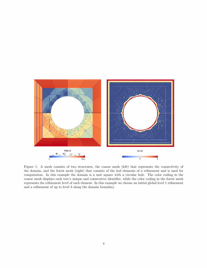
Figure 1: A mesh consists of two structures, the coarse mesh (left) that represents the connectivity ofthe domain, and the forest mesh (right) that consists of the leaf elements of a refinement and is used forcomputation. In this example the domain is a unit square with a circular hole. The color coding in thecoarse mesh displays each tree’s unique and consecutive identifier, while the color coding in the forest meshrepresents the refinement level of each element. In this example we choose an initial global level 1 refinementand a refinement of up to level 3 along the domain boundary.

4

f0f1

f20

2

1

0 1

2 3

f0 f1

f2

f3

4

10

32f0 f1f2

f3

f4f0

f1

f2

f3

0

1

23

0 1

2 3

4 5

6 7

f0 f1

f2

f3

f4

f5

f1

0 1

3 4

2

5

f0

f2f3

f4

Z

Y

X

Figure 2: The vertex and face labels of the 2D (left) and 3D (right) tree types.

2.2 Encoding of face-neighbors

The connectivity information of a coarse mesh includes the neighbor relation between adjacent trees. Twotrees are considered neighbors if they share at least one lower dimensional face (vertex, face, or edge). Sinceall of this connectivity information can be concluded from codimension-1 neighbors, we restrict ourselves tothose, denoting them uniformly by face-neighbors. At this point we do not consider neighbor relations acrosslower dimensional tree faces, as we believe without loss of generality for the partitioning algorithms to follow.

An application often requires a quick mechanism to access the face-neighbors of a given forest meshelement. If this neighbor element is a member of the same tree the computation can be carried out via the SFClogic, which involves only few bitwise operations for the cubical and tetrahedral Morton curves [11,12,26,42].If, however, the neighbor element belongs to a different tree, we need to identify this tree, given the parent treeof the original element and the tree face at which we look for the neighbor element. It is thus advantageousto store the face-neighbors of each tree in an array that is ordered by the tree’s faces. To this end, we fix theenumeration of faces and vertices relative to each other as depicted in Figure 2.

2.3 Orientation between neighbors

In addition to the global index of the neighbor tree across a face, we describe how the faces of the tree and itsneighbor are rotated relative to each other. We allow all connectivities that can be embedded in a compact3-manifold in such a way that each tree has positive volume. This includes the Moebius strip and Klein’sbottle and also quite exotic meshes, e.g. a cube whose one face connects to another in some rotation. Weobtain two possible orientations of a line-to-line connection, three for a triangle-to-triangle- and four for asquare-to-square connection.

We would like to encode the orientation of a face connection analogously to the way it is handled inp4est: At first, given a face f , its vertices are a subset of the vertices of the whole tree. If we order themaccordingly and re-numerate them consecutively starting from zero, we obtain a new number for each vertexthat depends on the face f . We call it the face corner number. If now two faces f and f ′ meet, the corner 0of the face with the smaller face number is identified with a face corner k in the other face. In p4est this kis defined to be the orientation of the face connection.

In order for this operation to be well-defined, it must not depend on the choice of the first face when thetwo face numbers are the same, which is easily verified for a single tree type. When two trees of differenttypes meet, we generalize to determine which face is the first one.

5

k0 k1

p0 p1 p1 p2

k0

k1

Figure 3: We patch multiple trees together to model complex geometries. Here, we show two trees k0 andk1 with an adaptive refinement. To store the forest mesh, we use a space-filling curve within each tree andthe a-priori tree order between trees. On the left-hand side of the figure the refinement tree and its linearstorage are shown. When we partition the forest mesh to P processes (here, P = 3), we cut the SFC in Pequal-size parts and assign part i to process i.

Definition 1. We impose a semiorder on the 3-dimensional tree types as follows:

Hexahedron<

Prism < Pyramid.

Tetrahedron<

(2)

This comparison is sufficient since a hexahedron and a tetrahedron can never share a common face. Weuse it as follows.

Definition 2. Let t and t′ denote the tree types of two trees that meet at a common face with respectiveface numbers f and f ′. Furthermore, let ξ be the face corner number of f ′ matching corner 0 of f and ξ′ theface corner number of f matching corner 0 of f ′. We define the orientation of this face connection as

or :=

{ξ if t < t′ or (t = t′ and f ≤ f ′),ξ′ otherwise.

(3)

We now encode the face connection in the expression or ·F + f ′ from the perspective of the first tree andor · F + f from the second, where F is the maximal number of faces over all tree types of this dimension.

3 Partitioning the coarse mesh

As outlined above, tree based AMR methods partition mesh elements with the help of an SFC. By cuttingthe SFC into as many equally sized parts as processes and assigning part i to process i, the repartitioningprocess is distributed and runs in linear time. Weighted partitions with a user defined weight per leaf elementare also possible and practical [12, 29].

If the physical domain has a complex shape such that many trees are required to optimally represent it,it becomes necessary to also partition the coarse mesh in order to reduce the memory footprint. This is evenmore important if the coarse mesh does not fit into the memory of one process, since such problems are noteven computable without coarse mesh partitioning.

Suppose the forest mesh is partitioned among the processes. Since the forest mesh frequently referencesconnectivity information from the coarse mesh, a process that owns a leaf e of a tree k also needs the

6

e0 e1

e2

e3

e7

e6

e5 e4

0

1

0

2

1

01

2

Figure 4: A coarse mesh of two trees and a uniform level 1 forest mesh. If the forest mesh is partitioned tothree processes, each tree of the coarse mesh is requested by two processes. The numbers in the tree cornersdenote the position and orientation of the tree vertices and the global tree ids are the numbers in the centerof each tree. As an example SFC we take the triangular Morton curve from [11], but the situation of multipletrees per process can occur for any SFC.

connectivity information of the tree k to its neighbor trees. Thus, we maintain information on these so-calledghost trees.

There are two traditional approaches to partition the coarse mesh. In the first approach [8,45], the coarsemesh is partitioned, and the owner process of a tree will own all elements of that tree. In other words, it isnot possible for two different processes to own elements of the same tree, which can lead to highly imbalancedforest meshes. Furthermore, if there are less trees then processes, there will be idle processes without anyleaf elements. In particular, this prohibits the frequently occurring special case of a single tree.

The second approach [47] is to first partition the forest mesh and to deduce the coarse mesh partitionfrom that of the forest. If several processes have leaf elements from the same tree, then the tree is assignedto one of these processes, and whenever one of the other processes requests information about this tree,communication is invoked. This technique has the advantage that the forest mesh is load balanced muchbetter, but it introduces additional synchronization points in the program and can lead to critical bottlenecksif a lot of processes request information on the same tree.

We propose another approach, which is a variation of the second, that overcomes the communication issue.If several processes have leaf elements from the same tree, we duplicate this tree’s connectivity data and storea local copy of it on each of this subset of processes. Thus, there is no further need for communication andeach process has exactly the information it requires. Since the purpose of the coarse mesh is not to storedata that changes during the simulation, but to store connectivity data about the physical domain thedata on each tree is persistent and does not change during the simulation. Certainly, this concept posesan additional challenge in the (re)partitioning process, because we need to manage multiple copies of treeswithout producing redundant messages.

As an example consider the situation in Figure 4. Here the 2D coarse mesh consists of two triangles 0 and1, and the forest mesh is a uniform level 1 mesh consisting of 8 elements. Elements 0, 1, 2, 3 are the childrenof tree 0 and elements 4, 5, 6, 7 the children of tree 1. If we load-balance the forest mesh to three processeswith ranks 0, 1 and 2, then a possible forest mesh partition arising from a SFC could be

rank elements0 0, 1, 21 3, 4, 52 6, 7,

(4)leading to the coarse mesh parti-tion

rank trees0 01 0, 12 1.

(5)

Thus, each tree is stored on two processes.

3.1 Valid partitions

We allow any SFC induced partition for the forest. This gives us some information on the type of coarsemesh partitions that we can expect as follows.

7

Definition 3. In general a partition of a coarse mesh ofK trees { 0, . . . ,K − 1 } to P processes { 0, . . . , P − 1 }is a map f that assigns each process a certain subset of the trees,

f : { 0, . . . , P − 1 } −→ P { 0, . . . ,K − 1 } , (6)

and whose image covers the whole mesh:

P−1⋃p=0

f(p) = { 0, . . . ,K − 1 } . (7)

Here, P denotes the set of all subsets (power set). We call f(p) the local trees of process p and explicitlyallow that f(p) ∩ f(q) may be nonempty. If so, the trees in this intersection are shared between processes pand q.

For a partition f we denote with kp the local tree on p with lowest global index and with Kp the one withthe highest global index.

We need not consider all possible partitions of a coarse mesh. Since we assume that a forest mesh partitioncomes from a space-filling curve, we can restrict ourselves to a subset of partitions.

Definition 4. Consider a partition f of a coarse mesh with K trees. We say that f is a valid partition ifthere exists a forest mesh with N leaves and a (possibly weighted) SFC partition of it that induces f . Thus,for each process p and each tree k we have k ∈ f(p) if and only if there exists a leaf e of the tree k in theforest mesh that is partitioned to process p. Processes without any trees are possible; in this case f(p) = ∅.

We deduce three properties that characterize valid partitions and lead to a definition that is independentof a forest mesh.

Proposition 5. A partition f of a coarse mesh is valid if and only if it fulfills the following properties.

(i) The tree indices of a process’ local trees are consecutive, thus

f(p) = { kp, kp + 1, . . . ,Kp } , or f(p) = ∅. (8)

(ii) A tree index of a process p may be smaller than a tree index on a process q only if p ≤ q:

p ≤ q ⇒ Kp ≤ kq (if f(p) 6= ∅ 6= f(q)). (9)

(iii) The only trees that can be shared by process p with other processes are kp and Kp:

f(p) ∩ f(q) ⊆ { kp,Kp } , for p 6= q. (10)

Proof. We show the only-if direction first. So let an arbitrary forest mesh with SFC partition be given, suchthat f is induced by it. In the SFC order the leaves are sorted according to their SFC indices. If (i, I) denotesthe leaf corresponding to the I-th leaf in the i-th tree and tree i has Ni leaves, then the complete forest meshconsists of the leaves

{ (0, 0), (0, 1), (0, N0 − 1), (1, 0), . . . , (K − 1, NK−1 − 1) } . (11)

The partition of the forest mesh is such that each process p gets a consecutive range{(kp, ip), . . . , (Kp, i

′p)}

(12)

8

of leaves. Where (kp+1, ip+1) is the successor of (Kp, i′p). and the kp and Kp form increasing sequences with

additionally Kp ≤ kp+1. The coarse mesh partition is then given by

f(p) = { kp, kp + 1, . . . ,Kp } , for all p, (13)

which shows properties (i) and (ii). To show (iii) we assume that f(p) has at least three elements, thusf(p) = { kp, kp + 1, . . . ,Kp }. However, this means that in the forest mesh partition each leaf that is a childfrom the trees in { kp + 1, . . . ,Kp − 1 } is partitioned to p. Since the forest mesh partitions are disjoint, noother process can hold leaf elements from these trees and thus they cannot be shared.

To show the if-direction, suppose the partition f fulfills (i), (ii) and (iii). We construct a forest meshwith a weighted SFC partition as follows. Each tree that is local to a single process is not refined and thus asingle leaf element in the forest mesh. If a tree is shared by m processes then we refine it uniformly until wehave more then m elements. It is now straightforward to choose the weights of the elements such that thecorresponding SFC partition induces f .

We directly conclude:

Corollary 6. In a valid partition each pair of processes can share at most one tree, thus

|f(p) ∩ f(q)| ≤ 1 (14)

for each p 6= q.

Proof. Suppose not then with (10) we know that there exist two processes p and q with p < q such thatf(p) ∩ f(q) = { kp,Kp } = { kq,Kq } and kp 6= Kp. Thus, Kp > kp = kq which contradicts property (9).

Corollary 7. If in a valid partition f of a coarse mesh the tree k is shared between processes p and q, thenfor each p < r < q

f(r) = { k } or f(r) = ∅. (15)

Proof. We can directly deduce this from (8), (9) and Corollary 6.

In order to properly deal with empty processes in our calculations, we define start and end tree indicesfor these as well.

Definition 8. Let p be an empty process in a valid partition f , thus f(p) = ∅. Let furthermore q < p bemaximal such that f(q) 6= ∅. Then we define the start and end indices of p as

kp := Kq + 1, (16)

Kp := Kq = kp − 1. (17)

If no such q exists, then no rank lower than p has local trees and we set kp = 0, Kp = −1. With thesedefinitions, equations (8) and (9) are valid if any of the processes are empty.

From now on all partitions in this manuscript are considered as valid even if not stated explicitly.

3.2 Encoding a valid partition

A typical way to define a partition in a tree based code is to store an array O of tree offsets for each process,that is, for process p the global index of the first local tree is stored. The range of local trees for process pcan then be computed as { O[p], . . . , O[p+ 1]− 1 }. However, for valid partitions in the coarse mesh setting,this information would not be sufficient because we would not know which trees are shared. We thus slightlymodify the offset array by adding a negative sign when the first tree of a process is shared.

9

Definition 9. Let f be a valid partition of a coarse mesh with kp being the index of p’s first local tree. Thenwe store this partition in an array O of length P + 1, where for 0 ≤ p < P

O[p] =

kp,if kp is not shared with the next smallernonempty process or f(p) = ∅,

−kp − 1, if it is.

(18)

Furthermore, in O[P ] we store the total number of trees.

Because of the definition of kp we know that O[0] = 0 for all valid partitions.

Lemma 10. Let f be a valid partition and O as in Definition 9. Then

kp =

{O[p], if O[p] ≥ 0,

|O[p] + 1|, if O[p] < 0,(19)

and

Kp = |O[p+ 1]| − 1. (20)

Proof. The first statement follows since equations (18) and (19) are inverses of each other.

For equation (20) we distinguish two cases: First, let f(p) be nonempty. If the last tree of p is not sharedwith p+ 1, then it is kp+1 − 1 and O[p+ 1] = kp+1, thus we have

Kp = kp+1 − 1 = |O[p+ 1]| − 1. (21)

If the last tree of p is shared with p+1, then it is kp+1, the first local tree of p+1 and thus O[p+1] = −kp+1−1and

Kp = kp+1 = | − kp+1| = |O[p+ 1]| − 1. (22)

Let now f(p) = ∅. If kp+1 is not shared, then kp+1 = kp = Kp + 1 by Definition 8 and O[p + 1] = kp+1 by(18). Thus,

Kp = kp − 1 = kp+1 − 1 = |O[p+ 1]| − 1. (23)

If kp+1 is shared, then again by Definition 8 kp+1 = kp − 1 = Kp and O[p + 1] = −kp+1 − 1, such that weobtain

Kp = kp+1 = kp+1 + 1− 1 = |O[p+ 1]| − 1. (24)

Corollary 11. In the setting of Lemma 10 the number np of local trees of process p fulfills

np = |O[p+ 1]| − kp =

{|O[p+ 1]| − O[p], if O[p] ≥ 0

|O[p+ 1]| − |O[p] + 1|, else.(25)

Proof. This follows from the formula np = Kp − kp + 1.

Lemma 10 and Corollary 11 show that for valid partitions the array O carries the same information as thepartition f .

10

3.3 The ghost trees

A valid partition gives the information about the local trees of a process. These trees are all trees from whoma forest has local elements. In many applications it is necessary to create a layer of ghost (or halo) elementsof the forest to properly exchange data with the neighboring processes. Since these ghost elements may bedescendants of non local trees, we also want to store those trees as ghost trees. To be independent of a forestmesh we store each possible ghost tree and do not consider whether there are actually forest mesh ghostelements in this tree. This, however, does only affect the first and the last local tree, where we possibly storemore ghosts than needed by a forest. Since we restrict the neighbor information to face-neighbors, we alsorestrict ourselves to face-neighbor ghosts in this paper.

Definition 12. Let f be a valid partition of a coarse mesh. A ghost tree of a process p is any tree k suchthat

• k /∈ f(p), and

• There exists a face-neighbor k′ of k, such that k′ ∈ f(p).

If a coarse mesh is partitioned according to f then each process p will store its local trees and its ghosttrees.

3.4 Computing the communication pattern

Suppose we are in a setting where a coarse mesh is partitioned among the processes p ∈ { 0, . . . , P − 1 }according to a partition f . The input of the partition algorithm is this coarse mesh and a second partitionf ′, and the output is a coarse mesh that is partitioned according to the second partition.

We suppose that besides its local trees and ghosts each process knows the complete partition tables f andf ′, for example in the form of offset arrays. The task is now for each process to identify the processes that itneeds to send local trees and ghosts to and carry out this communication. A process also needs to identifythe processes it receives trees and ghosts from and do the receiving. We discuss here how each process cancompute this information from the offset arrays without further communication.

3.4.1 Ownership during partition

The fact that trees can be shared between multiple processes poses a challenge when repartitioning a coarsemesh. Suppose we have a process p and a tree k with k ∈ f ′(p), and k is a local tree for more than one processin the partition f . We do not want to send the tree multiple times, so how do we decide which process sendsk to p?

A simple solution would be that the process with the smallest index that k is a local tree to sends k.This process is unique and it can be determined without communication. However, suppose that the twoprocesses p and p− 1 share the tree k in the old partition and p will also have this tree in the new partition.Then p− 1 would send the tree to p even though we could handle this situation without any communication.

We solve this by only sending a local tree to a process p if this tree was not already local on p:

Paradigm 13. In a repartitioning setting with k ∈ f ′(p), the process that sends k to p is

• p, if k already is a local tree of p, or else

• q, with q minimal such that k ∈ f(q).

We acknowledge that sending from p to p in the first case is just a local data movement involving nocommunication.

11

Definition 14. In a repartitioning setting, given a process p we define the sets Sp and Rp of processes thatp sends local trees to, resp. receives from, thus

Sp := { 0 ≤ p < P | p sends local trees to p’ } , (26a)

Rp := { 0 ≤ p < P | p receives local trees from p’ } . (26b)

These sets can both include the process p itself. Furthermore, we establish notations for the smallest andbiggest ranks in these sets:

sfirst := minSp, slast := maxSp, (27a)

rfirst := minRp, rlast := maxRp. (27b)

Sp and Rp are uniquely determined by Paradigm 13.

3.4.2 An example

We discuss a small example, see Figure 5. Here, we repartition a partitioned coarse mesh of five trees amongthree processes. We color the local trees of process 0 in blue, the local trees of process 1 in green and thelocal trees of process 2 in red. The initial partition f is given by

O = { 0,−2, 3, 5 } , (28)

and the new partition f ′ by

O’ = { 0,−3,−4, 5 } . (29)

Thus, initially tree 1 is shared by processes 0 and 1 and in the new partition tree 2 is shared by processes0 and 1 and tree 3 by processes 2 and 3. We give the local trees that each process will send to each otherprocess in a table, where the set in row i column j is the set of local trees that process i send to process j.

0 1 20 { 0, 1 } ∅ ∅1 { 2 } { 2 } ∅2 ∅ { 3 } { 3, 4 }

(30)

This leads to the sets Sp and Rp:

S0 = { 0 } , R0 = { 0, 1 } , (31a)

S1 = { 0, 1 } , R1 = { 1, 2 } , (31b)

S2 = { 1, 2 } , R2 = { 2 } . (31c)

For example process 1 keeps the tree 2 that is also needed by process 0. Thus, process 1 sends tree 2 toprocess 0. Process 0 also needs tree 1, which is local on process 1 in the old partition. But, since it is alsolocal to process 0, process 1 does not send it.

3.4.3 Determining Sp and Rp

In this section we show that each process can compute the sets Sp and Rp from the offset array withoutfurther communication. It will become clear in Section 3.5 that ghost trees need not yet be discussed at thispoint.

12

0

1

2

34

Figure 5: A small example for coarse mesh partitioning. The coarse mesh consists of 5 trees and is partitionedamong three processes. Left: The initial partition O. Right: The new partition O’. The colors of the treesencode the processes that have the respective tree as local tree. Process 0 in blue, process 1 in green, andprocess 2 in red. Thus, initially tree 1 is shared among processes 0 and 1 and in the new partition tree 2 isshared among processes 0 and 1, and tree 3 among processes 1 and 2. In equations (28)-(31) we depict thesets O and O’, the trees that each process sends, and the sets Sp and Rp.

Proposition 15. A process p can calculate the sets Sp and Rp without further communication from the offsetarrays of the new and old partition. Once the first and last element of each set are known, p can determinein constant time whether any given rank is in any of those sets.

We split the proof in two parts. First we discuss how a process can compute sfirst, slast, rfirst, and rlast,and then how it can decide for two processes p and q whether q ∈ Sp.

We derive Sp from sfirst and slast. To determine sfirst we consider two cases. First, if the first local tree ofp is not shared with a smaller rank, then sfirst is the smallest process that has this tree in the new partitionand did not have it in the old one. We can find this process with a binary search in the offset array.

Second, if the first tree of p is shared with a smaller rank, then p only sends it in the case that p keepsthis tree in the new partition. Then sfirst = p. Otherwise, we consider the second tree of p and proceed witha binary search as in the first case.

To compute slast we notice that among all ranks having p’s old last tree in the new partition that did notalready have it before, slast is the biggest (except when p itself is this biggest rank, in which case it certainlyhad the last tree before). We can determine this rank with a binary search as well. If no such process exists,we proceed with the second last tree of p.

Remark 16. The special case when Sp = ∅ occurs under three circumstances:

1. p does not have any local trees.

2. p only has one local tree, it is shared with a smaller rank, and p does not have this tree as a local treein the new partition.

3. p only has two trees, for the first one case 2 holds and the second (=last) one is shared with a set Q ofbigger ranks. There is no process q /∈ Q that has this tree as a local tree in the new partition.

These conditions can be queried before computing sfirst and slast.

Similarly, to compute Rp, we first look at the smallest and biggest elements of this set. These are the firstand last process that p receives trees from. rfirst is the smallest rank that had p’s new first tree as a localtree in the old partition, or it is p itself if this tree was also a local tree on p. And rlast is the smallest rankbigger then rfirst that had p’s new last local tree as a local tree in the old partition, or p itself. We can findboth of these with a binary search in the offset array of the old partition.

13

Remark 17. Rp is empty if and only if p does not have any local trees in the new partition.

Lemma 18. Given any two processes p and q the process p can determine in constant time whether q ∈ Sp.In particular, this includes the cases p = p and q = p.

Proof. Let kp be the first non-shared local tree of p in the old partition. Let Kp be the last local tree of p inthe old partition if it is not the first local tree of q in the old partition. Let it be the second last local treeotherwise. Furthermore, let kq and Kq be the first, resp. last, local trees of q in the new partition. We add

1 to kq if q sends its first local tree to itself and this tree is also the new first local tree of q. We claim thatq ∈ Sp if and only if all of the four inequalities

kp ≤ Kp, kp ≤ Kq, kq ≤ Kp, and kq ≤ Kq (32)

hold. The only-if direction follows, since if kp > Kp, then p does not have trees to send to q. If kp > Kq,

then the last new tree on q is smaller than the first old tree on p. If kq > Kp then the last tree that p could

send is smaller than the first new local tree of p. And if kq > Kq then q does not receive any trees from otherprocesses. Thus p cannot send trees to q if any of the four conditions is not fulfilled. The if-direction follows,since if all four conditions are fulfilled there exist at least one tree k with

kp ≤ k ≤ Kp and kq ≤ k ≤ Kq. (33)

Any tree with this properties is sent from p to q. Process p can compute the four values kp, Kp, kq and Kq

from the partition offsets in constant time.

Remark 19. Let p be a process that is not empty in the new partition. For symmetry reasons, Rp containsexactly those processes p with rfirst ≤ p ≤ rlast and p ∈ Sp.

Thus, in order to compute Sp, we can compute sfirst and slast and then check for each rank q in betweenwhether the conditions of Lemma 18 are fulfilled with p = p. For each process this check only takes constantrun time.

Now, to compute Rp we can compute rfirst and rlast, and then check for each rank q in between whetherp ∈ Sq.

These considerations provide the proof for Proposition 15.

3.5 Face information for ghost trees

We identify five different types of possible face connections in a coarse mesh:

1. Local tree to local tree.

2. Local tree to ghost tree.

3. Ghost tree to local tree.

4. Ghost tree to ghost tree.

5. Ghost tree to non-local and non-ghost tree.

There are several possible approaches to which of these face connections of a local coarse mesh we couldactually store. As long as each face connection between any two neighbor trees is stored at least once globally,the information of the coarse mesh over all processes is complete, and a single process could reproduce allfive types of face connection at any time, possibly using communication. Depending on which of these typeswe store, the pattern for sending and receiving ghost trees during repartitioning changes. Specifically, thetrees that will become a ghost on the receiving process may be either a local tree or a ghost on the sendingprocess.

When we use the maximum possible information of all five connections, we have the most data availableand can minimize the communication required. In particular, from the non-local neighbors of a ghost and

14

the partition table a process can compute which other processes this ghost is also a ghost of and of which itis a local tree. With this information we can ensure that a ghost is only sent once and only from a processthat also sends local trees to the receiving process.

The outline of the sending/receiving phase of the partition algorithm then looks like this:

1. For each q ∈ Sp: Send local trees that will be owned by q (following Paradigm 13).

2. Consider sending a neighbor of these trees to q if it will be a ghost on q. Send one of these neighborsif both

• p is the smallest rank among those that consider sending this neighbor as a ghost, and

• p 6= q and q does not consider sending this neighbor as a ghost to itself.

3. For each q ∈ Rp: Receive the new local trees and ghosts from q.

In step 2 a process needs to know, given a ghost that is considered for sending to q, which other processesconsider sending this ghost to q. This can be calculated without further communication from the face-neighbor information of the ghost. Since we know for each ghost the global index of each of its neighbors,we can check whether any of these neighbors is currently local on a different process p and will be sent to qby p. If so, we know that p considers sending this ghost to q.

Using this method, each local tree and ghost is sent only once to each receiver, and only those processessend that send local trees anyway, thus we have a minimum number of communications and data movement.Storing less information would either increase the number of communicating processes or the amount of datathat is communicated.

Suppose we would not store the face connection type 5, thus for ghost trees we do not have the informationwith which non-local trees it is connected. With this face information we can use a communication patternsuch that each ghost is only received once by a process q, by sending the new ghost trees from a process thatcurrently has it as a local tree (taking Paradigm 13 into account). However, this designated process mightnot be an element of Rq, in which case additional processes would communicate.

If we only store the local tree face information, types 1 and 2, then we have minimal control over the ghostface connections. Nevertheless, we can define the partition algorithm by specifying that if a process p sendslocal trees to a process q, it will send all neighbors of these local trees as potential ghosts to q. The processq is then responsible for deleting those trees that it received more than once. With this method the numberof communicating processes would be the same but the amount of data communicated would increase.

We give an example comparing the three face information strategies in Figure 6. To minimize the com-munication and overcome the need for postprocessing steps, it is thus recommended to store all five types offace connections.

4 Implementation

Let us begin by outlining the main data structures for trees, ghosts, and the coarse mesh, and continue witha section on how to update the local tree and ghost indices. After this we present the partition algorithm torepartition a given coarse mesh according to a pre-calculated partition array. We emphasize that the coarsemesh data stores pure connectivity. In particular, it does not include the forest information, that is leafelements and per-element payloads, which are managed by separate, existing algorithms.

4.1 The coarse mesh data structure

Our data structure cmesh that describes a (partitioned) coarse mesh has the entries:

• O — An array storing the current partition table, see Definition 9.

15

0 1

1

0 1

2

0 1

2

0,1 1

2

1, 2 1, 2, 3, 4 1, 2, 3, 4, 5p 0 1 2 0 1 2 0 1 20 0(1,2) 0(2) — 0 0 (0) 0(1,2) 0 —

1 — 1(2) 2(0,1) (1,2) 1(2) 2(1) — 1(2) 2 (0,1)

Figure 6: Repartitioning example of a coarse mesh showing the communication patterns controlled by theamount of face information available. Top: A coarse mesh of three trees is repartitioned. The numbersoutside of the trees are their global indices. The numbers inside of each tree denote the processes that havethis tree as a local tree. At first process 0 has tree 0, process 1 trees 1 and 2, and process 2 no trees as localtrees. After repartitioning process 0 has tree 0, process 1 trees 0 and 1, and process 2 tree 2 as local trees.Bottom: The table shows for each usage of face connection types which processes send which data. The rowof process i shows in column j which local trees i sends to j, and—in parentheses—which ghosts it sends toj. Using face connection types 1–4 we use more communication partners (process 0 sends to process 2 andprocess 1 to process 0) than with all five types. Using types 1 and 2 only, duplicate data is sent (process 0and process 1 both send the ghost tree 2 to process 1).

16

• np — The number of local trees on this process.

• nghosts — The number of ghost trees on this process.

• trees — A structure storing the local trees in order of their global index.

• ghosts — A structure storing the ghost trees in no particular order.

We use 32-bit signed integers for the local tree counts in trees and ghosts and 64-bit integers for globalcounts in O. This limits the number of trees per process to 231 − 1 ∼= 2× 109. However, even with an overlyoptimistic memory usage of only 10 bytes per tree, storing that many trees would require about 18.6GB ofmemory per process. Since on most distributed machines the memory per process is indeed much smaller,restricting to 32-bit integers does not effectively limit the local number of trees. In presently unimaginablecases, we can still switch to 64-bit integers.

We call the index of a local tree inside the trees array the local index of this tree. Analogously, we callthe index of a ghost in ghosts the local index of that ghost. On process p, we compute the global index k ofa tree in trees from its local index ` and the global index kp of the first local tree and vice versa, since

k = kp + `. (34)

This allows us to address local trees with their local indices using 32-bit integers.

Each tree in the array trees stores the following data:

• eclass — The tree’s type as a small number (triangle, quadrilateral, etc.).

• tree to tree — An array storing the local tree and ghost neighbors along this tree’s faces. See Section2.2.

• tree to face — An array encoding for each face the neighbor face number and the orientation of theface connection. See Section 2.3.

• tree data — A pointer to additional data that we store for the tree, for example geometry informationor boundary conditions defined by an application.

The i-th entry of tree to tree array encodes the tree number of the face-neighbor at face i using aninteger k with 0 ≤ k < np + nghosts. If k < np, the neighbor is the local tree with local index k. Otherwisethe neighbor is the ghost with local index k − np.

We do not allow a face to be connected to itself. Instead, we use such a connection in the face-neighborarray to indicate a domain boundary. However, a tree can be connected to itself via two different faces. Thisallows for one-tree periodicity, as say in a 2D torus consisting of a single square tree.

Each ghost in the array ghosts stores the following data:

• Id — The ghost’s global tree index.

• eclass — The type of the ghost tree.

• tree to tree — An array giving for each face the global number of its face-neighbor.

• tree to face — As above.

Since a ghost stores the global number of all of its face-neighbor trees, we can locally compute all otherprocesses that have this tree as a ghost by combining the information from O and tree to tree.

17

4.2 Updating local indices

After partitioning, the local indices of the trees and ghosts change. The new local indices of the local treesare determined by subtracting the global index of the first local tree from the global index of each local tree.The local indices of the ghosts are given by their position in the data array.

Since the local indices change after repartitioning, we update the face-neighbor entries of the local treesto store those new values. Because a neighbor of a tree can either be a local tree or a ghost on the previouslyowning process p and become either a tree or a ghost on the new owning process p, there are four cases thatwe shall consider.

We handle these four cases in two phases, the first phase is carried out on process p before the tree is sentto p. In this phase we change all neighbor entries of the trees that become local. The second phase is doneon p after the tree was received from p. Here we change all neighbor entries belonging to trees that becomeghosts.

In the first phase, p has information about the first local tree on p in the old partition, its global numberbeing kp. Via O’ it also knows knew

p , the global index of p’s first tree in the new partition. Given a local tree

on p with local index k in the old partition we compute its new local index k on p as

k = kp + k − knewp , (35)

which is its global index minus the global index of the new first local tree. Given a ghost g on p that will bea local tree on p, we compute its local tree number as

k = g.Id− knewp . (36)

In the second phase p, has received all its new trees and ghosts and thus can give the new ghosts localindices to be stored in the neighbors fields of the trees. We do this by parsing, for each process p ∈ Rp (inascending order), its ghosts and increment a counter. For each ghost we parse its neighbors for local trees,and for any of these we set the appropriate value in its neighbors field.

4.3 Partition cmesh — Algorithm 4.1

The input is a partitioned coarse mesh C and a new partition layout O’, and the output is a new coarse meshC ′ that carries the same information as C and is partitioned according to O’.

This algorithm follows the method described in Section 3.5 and is separated in two main phases, thesending phase and the receiving phase. In the former we iterate over each process q ∈ Sp and decidewhich local trees and ghosts we send to q. Before sending, we carry out phase one of the update of the localtree numbers. Subsequently, we receive all trees and ghosts from the processes in Rp and carry out phasetwo of the local index updating.

In the sending phase we iterate over the trees that we send to q. For each of these trees we check foreach neighbor (local tree and ghost) whether we send it to q as a ghost tree. This is the item 2 in the listof Section 3.5. The function Parse neighbors decides for a given local tree or ghost neighbor whether it issent to q as a ghost.

5 Numerical Results

The run time results that we present here have been obtained using the Juqueen supercomputer at Forschungszen-trum Julich, Germany. It is an IBM BlueGene/Q system with 28,672 nodes consisting of IBM PowerPC A2processors at 1.6 GHZ with 16 GB RAM per node [14]. Each compute node has 16 cores and is capable ofrunning up to 64 MPI processes using multithreading.

18

Algorithm 4.1: Partition cmesh(cmesh C, partition O’)

1 p← this process2 From C.O and O’ determine Sp and Rp. /* See Section 3.4.3 */

/* Sending phase */

3 for each q ∈ Sp do4 G← ∅ /* trees p sends as ghosts to q */

5 s← first local tree to send to q.6 e← last local tree to send to q.7 T ← {C.trees[s], . . . , C.trees[e] } /* local trees p sends to q */

8 for k ∈ T do9 Parse neighbors (C, k, p, q, G, O’)

10 update tree ids phase1 (T ∪G) /* See equations (35) and (36) */

11 Send T ∪G to process q

/* Receiving phase */

12 for each q ∈ Rp do13 Receive T [q] ∪G[p] from process p

14 C′.trees←⋃Rp

T [q] /* The updated tree array */

15 C′.ghosts←⋃Rp

G[q] /* The updated ghost array */

16 update tree ids phase2 (C.ghosts)17 C′.O← O’

18 return C’

/* decide which neighbors of k to send as a ghost to q */

1 Function Parse neighbors(cmesh C, tree k, processes p, q, Ghosts ∗G, partition O’)2 for u ∈ k.tree to tree\ {C.trees[s], . . . , C.trees[e] } do3 if 0 ≤ u < kp and Send ghost(C, ghost(u), q, O’) then4 if u + kp /∈ f ′(q) then5 G← G ∪ { ghost(u) } /* local tree u gets ghost of q */

6 else /* kp ≤ u */

7 g ← C.ghosts[u− np] if g.Id /∈ f(q) and Send ghost(C, g, q, O’) then8 G← G ∪ { g } /* g is a ghost of q */

/* Subroutine to decide whether to send a ghost or not */

1 Function Send ghost(cmesh C, ghost g, process q, partition O’) S ← ∅2 for u ∈ g.tree to tree do3 for q′ with u is a local tree of q′ do4 if q′ sends u to q then5 S ← S ∪ { q′ }

6 if q /∈ S and p = minS then7 return True /* p is the smallest rank sending trees to q */

8 else9 return False

19

5.1 How to obtain example meshes

To measure the performance and memory consumption of the algorithms presented above, we would like totest the algorithms on coarse meshes that are too big to fit into the memory of a single process, which is 1GB on Juqueen if we use 16 MPI ranks per node. We consider three approaches to do construct such meshes:

1. Use an external parallel mesh generator.

2. Use a serial mesh generator on a large-memory machine, transfer the coarse mesh to the parallelmachine’s file system, and read it using (parallel) file I/O.

3. Create a big coarse mesh by forming the disjoint union of smaller coarse meshes over the individualprocesses.

Due to a lack of availability of open source parallel mesh generators we restrict ourselves to the secondand third method. These have the advantage that we can start with initial coarse meshes that fit into asingle process’ memory, such that we can work with serial mesh generating software. In particular we usegmsh, Tetgen and Triangle for simplicial meshes [19,35,36].

The third method is especially well suited for weak scaling studies. The small coarse meshes can be createdprogrammatically, communication-free on each process, which we exploit below for tests with hexahedral trees.They may be of same or different sizes between the processes. In the former approach, the number of localtrees is, by definition, the same on each process.

We discuss two examples below: one examining purely the coarse mesh partitioning without regard fora forest and its elements, and another in which we drive the coarse mesh partitioning by a dynamicallychanging forest of elements. The latter manages shared trees and thus fully executes the algorithmic ideasput forward above.

5.2 Disjoint bricks

In our first example we conduct a strong and weak scaling study of coarse mesh partitioning and test themaximal number of cubical trees that we can support before running out of memory. To obtain reliable weakscaling results, we keep the same per-process number of trees while increasing the total number of processes.We achieve this by constructing an nx × ny × nz brick of cubical trees on each process, using three constantparameters nx, ny and nz. We repartition this coarse mesh once, by the rule that each rank p sends 43% ofits local trees to the rank p + 1 (except the biggest rank P − 1, which keeps all its local trees). We choosethis odd percentage to create non-trivial boundaries between the regions of trees to keep and trees to send.See Figure 7 for a depiction of the partitioned coarse mesh on six processes. The local bricks are createdlocally as p4est connectivities with p4est connectivity new brick and are then reinterpreted in parallelas a distributed coarse mesh data structure.

We perform strong and weak scaling studies on up to 917,504 MPI ranks and display our results inFigures 8 and 9 and Table 1. We show the results of one study with 16 MPI ranks per compute node,thus 1GB available memory per process, and one with 32 MPI ranks per compute node, leaving half of thememory per process. In both cases we measure run times for different mesh sizes per process. We observethat even for the biggest meshes of 405k resp. 810k coarse mesh elements per process the absolute run timesof partition are below 1.2 seconds. Furthermore, we measure a weak scaling efficiency of 97.4% for the 810kmesh on 262,144 processes and 86.2% for the 405k mesh on 458,752 processes. The biggest mesh that wecreated is partitioned between 917,504 processes and uses 405k mesh elements per process for a total of over371e9 coarse mesh elements.

Additionally, in Table 2 we show run times for Partition cmesh with small coarse meshes, where thenumber of elements is roughly on the order of the number of processes. These tests show that for such smallmeshes the run times are in the order of milliseconds. Hence, for small meshes there is no disadvantage inusing a partitioned coarse mesh over a replicated one, when each process holds a full copy.

20

Figure 7: Depicting the structure of the coarse mesh for an example with six processes that we use to measurethe maximum possible mesh sizes and scalability. Before partitioning, the coarse mesh local to each processis created as one nx × ny × nz block of cubical trees. We repartition the mesh such that each process sends43% of its local trees to the next process. The picture shows the resulting partitioned coarse mesh withparameters nx = 10, ny = 18 and nz = 8 and color coded MPI rank.

0.115

0.23

0.37

0.62

1.12

16384 32768 65536 131072 262144 458752

Runtime[s]

Number of MPI ranks

weak scaling with 16 ranks/node

0.115

0.23

0.37

0.62

1.12

16384 32768 65536 131072 262144 458752

Runtime[s]

Number of MPI ranks

weak scaling with 16 ranks/node

K/P = 50625K/P = 101250K/P = 202500K/P = 405000K/P = 810000

0.166

0.28

0.41

0.75

1.19

32768 65536 131072 262144 524288 917504

Runtime[s]

Number of MPI ranks

weak scaling with 32 ranks/node

0.166

0.28

0.41

0.75

1.19

32768 65536 131072 262144 524288 917504

Runtime[s]

Number of MPI ranks

weak scaling with 32 ranks/node

K/P = 50625K/P = 101250K/P = 202500K/P = 405000

Figure 8: Weak scaling of partition with disjoint bricks. Left: 16 ranks per node. Right: 32 ranks pernode. We show the run times for the baseline on the y-axis. On the left hand side the run time for thebiggest 262,144-process run is 1.15 seconds, and the run time for the biggest 458,752 run is 0.719 seconds.We obtain an efficiency of 97.4%, resp. 86.2% compared to the baseline of 16,384 MPI ranks.

21

0.3

0.5

0.75

1

16384 32768 65536 131072 262144 458752

Par

alle

leffi

cien

cy[%

]

Number of MPI ranks

0.3

0.5

0.75

1

16384 32768 65536 131072 262144 458752

Par

alle

leffi

cien

cy[%

]

Number of MPI ranks

K = 1.33e10K = 2.65e10K = 5.31e10

0.8

1

2

4

8

16384 32768 65536 131072 262144

Speedup

Number of MPI ranks

0.8

1

2

4

8

16384 32768 65536 131072 262144

Speedup

Number of MPI ranks

K = 1.33e10K = 2.65e10K = 5.31e10ideal speedup

Figure 9: Strong scaling of Partition cmesh for the disjoint bricks example on Juqueen with 16 ranks percompute node, for three runs with 1.33e10, 2.65e10, and 5.31e10 coarse mesh elements. We show the parallelefficiency on the left and the speedup on the right. The absolute run times for 262,144 processes are 0.206,0.270 and 0.380 seconds.

Run time tests for Partition cmesh

131072 MPI ranks (16 ranks per node)

mesh size per rank trees (ghosts) sent Time [s] Factor

6,635e9 50,625 21,768 (3,414) 0.13 –1,327e10 101,250 43,537 (5,504) 0.20 1.532,654e10 202,500 87,074 (6,607) 0.31 1.565,308e10 405,000 174,149 (11,381) 0.57 1.851,062e11 810,000 348,297 (22,335) 1.08 1.89

917504 MPI ranks (32 ranks per node)

mesh size per rank trees (ghosts) sent Time [s] Factor

4.645e10 50,625 21,768 (3,413) 0.64 –

9.290e10 101,250 43,537 (5,504) 0.72 1.13

1.858e11 202,500 87,075 (6,607) 0.84 1.12

3,716e11 405.000 174,150 (11,383) 1.19 1.42

Table 1: The run times of Partition cmesh for 131,072 processes with 16 processes per node (top) and917,504 processes with 32 processes per node (bottom). The biggest coarse mesh that we created during thetests has 371 Billion trees. The last column is the quotient of the current run time divided by the previousrun time. Since we double the mesh size in each step, we would expect an increase in run time of a factor of2, which hints at parallel overhead becoming negligible in the limit of many elements per process.

22

# MPI ranks mesh elements run time [s]1024 4096 0.001361024 8192 0.001491024 16384 0.00142

64 105 0.0012232 105 0.0078964 3200 0.00029364 19200 0.000865

Table 2: Run times for Partition cmesh for relatively small coarse meshes. The bottom part of the tablewas not computed on Juqueen but on a local institute cluster of 78 nodes with 8 Intel Xeon CPU E5-2650v2 @ 2.60GHz each.

5.3 An example with a forest

In this example we partition a tetrahedral coarse mesh according to a parallel forest of fine elements. Opposedto the previous test, where we exploited the maximum possible coarse element numbers, we now test meshsizes that can occur in realistic use cases.

When simulating shock waves or two-phase flows, there is often an interface along which a finer meshresolution is desired in order to minimize computational errors. Motivated by this example, we create theforest mesh as an initial uniform refinement of the coarse mesh with a specified level ` and refine it in a bandalong an interface defined by a plane in R3 up to a maximum refinement level `+k. As refinement rule we use1:8 red refinement [6] together with the tetrahedral Morton space-filling curve [11]. We move the interfacethrough the domain with a constant velocity. Thus, in each time step the mesh is refined and coarsened, andtherefore we repartition it to maintain an optimal load-balance. We measure run times for both coarse meshand forest mesh partitioning for three time steps.

Our coarse mesh consists of tetrahedral trees modelling a brick with spherical holes in it. To be moreprecise, the brick is built out of nx × ny × nz tetrahedralized unit cubes and each of those has one sphericalhole in it; see Figures 10 and 11 for a small example mesh.

We create the mesh in serial using the generator gmsh [19]. We read the whole file on a single process, andthus use a local machine with 1 terabyte memory for preprocessing. On this machine we partition the coarsemesh to several hundred processes and write one file for each partition. This data is then transferred to thesupercomputer. The actual computation consists of reading the coarse mesh from files, creating the forest onit, and partitioning the forest and the coarse mesh simultaneously. To optimize memory while loading thecoarse mesh, we open at most one partition file per compute node.

The coarse mesh that we use in these tests has parameters nx = 26, ny = 24, nz = 18, thus 11,232 unitcubes. Each cube is tetrahedralized with about 34,150 tetrahedra, and the whole mesh consists of 383,559,464trees. In the first test, we create a forest of uniform level 1 and maximal refinement level 2, and in the seconda forest of uniform level 2 and maximal refinement level 3. The forest mesh in the first test consists ofapproximately 2.6e9 elements. In the second test we also use a broader band and obtain a forest mesh of25e9 tetrahedra.

We show the run time results and further statistics for coarse mesh partitioning in Table 3 and resultsfor forest partitioning in Table 4. We observe that the run time for Partition cmesh is between 0.10 and0.13 seconds, and that about 88%, respectively 98%, of all processes share local trees with other processes.The run times for forest partition are below 0.22 seconds for the first example and below 0.65 seconds for thesecond example. Thus, the overall run time for a complete mesh partition is below 0.5 seconds for the firstand below 1 second for the second example.

We also run a third test on 458,752 MPI ranks and refine the forest to a maximum level of four. Here,the forest mesh has 167e9 tetrahedra, which we partition in under 0.6 seconds. The coarse mesh partition

23

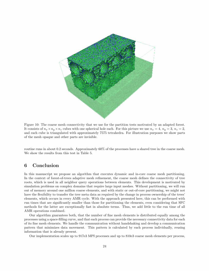
Figure 10: The coarse mesh connectivity that we use for the partition tests motivated by an adapted forest.It consists of nx×ny×nz cubes with one spherical hole each. For this picture we use nx = 4, ny = 3, nz = 2,and each cube is triangulated with approximately 7575 tetrahedra. For illustration purposes we show partsof the mesh opaque and other parts are invisible.

routine runs in about 0.2 seconds. Approximately 60% of the processes have a shared tree in the coarse mesh.We show the results from this test in Table 5.

6 Conclusion

In this manuscript we propose an algorithm that executes dynamic and in-core coarse mesh partitioning.In the context of forest-of-trees adaptive mesh refinement, the coarse mesh defines the connectivity of treeroots, which is used in all neighbor query operations between elements. This development is motivated bysimulation problems on complex domains that require large input meshes. Without partitioning, we will runout of memory around one million coarse elements, and with static or out-of-core partitioning, we might nothave the flexibility to transfer the tree meta data as required by the change in process ownership of the trees’elements, which occurs in every AMR cycle. With the approach presented here, this can be performed withrun times that are significantly smaller than those for partitioning the elements, even considering that SFCmethods for the latter are exceptionally fast in absolute terms. Thus, we add little to the run time of allAMR operations combined.

Our algorithm guarantees both, that the number of fine mesh elements is distributed equally among theprocesses using a space-filling curve, and that each process can provide the necessary connectivity data for eachof its fine mesh elements. We handle the communication without handshaking and develop a communicationpattern that minimizes data movement. This pattern is calculated by each process individually, reusinginformation that is already present.

Our implementation scales up to 917e3 MPI processes and up to 810e3 coarse mesh elements per process,

24

Figure 11: An illustration of the band of finer forest mesh elements in the example. The region of finer meshelements moves through the mesh in each time step. From left to right we see t = 1, t = 2, and t = 3. Inthis illustration, elements of refinement level 1 are blue and elements of refinement level 2 are red.

Coarse mesh partition on 8,192 MPI ranks

t trees (ghosts) sent data sent [MiB] |Sp| shared trees run time [s]1 25,116.7 (11,947.5) 4.945 2.274 7178 0.1032 34,860.3 (16,854.9) 6.880 2.753 7176 0.1103 36,386.0 (17,567.6) 7.180 2.823 7182 0.1121 39,026.2 (18,333.9) 7.670 2.962 8096 0.1282 38,990.1 (18,268.0) 7.660 2.946 8085 0.1293 38,941.7 (18,073.9) 7.639 2.933 8085 0.128

Table 3: Partition cmesh with a coarse mesh of 324,766,336 tetrahedral trees on 8192 MPI ranks. Wemeasure mesh repartition for three time steps. For each we show process average values of the number oftrees ghosts, and total number of bytes that each process sends to other processes. The average number ofother processes to which a process sends (|Sp|) is in each test below three. We also give the total number ofshared trees in the mesh, 8191 being the maximum possible value. We round all numbers to three significantfigures. 1 MiB = 10242 bytes.

Forest mesh partition on 8,192 MPI ranks

t mesh size elements sent data sent [MiB] run time [s]1 2,622,283,453 203,858 3.494 0.2152 2,623,842,241 281,254 4.824 0.2153 2,626,216,984 293,387 5.032 0.2141 25,155,319,545 3,013,230 46.574 0.6422 25,285,522,233 3,008,800 46.506 0.6403 25,426,331,342 2,991,990 46.248 0.645

Table 4: For the same example as in Table 3 we display statistics and run times for the forest mesh partition.We show the total number of tetrahedral elements, and the average count of elements and bytes that eachprocess sends to other processes (their count is the same as in Table 3). We round all numbers to threesignificant figures.

25

Coarse mesh partition on 458,752 MPI ranks

t trees (ghosts) sent data sent [MiB] |Sp| shared trees run time [s]1 703.976 (2444.11) 0.267 2.986 280,339 0.2072 707.368 (2455.95) 0.269 2.996 281,694 0.2043 707.904 (2457.70) 0.269 2.997 281,900 0.204

Forest mesh partition on 458,752 MPI ranks

t mesh size elements sent data sent [MiB] run time [s]1 167,625,595,829 362,863 5.548 0.5222 167,709,936,554 364,778 5.577 0.5783 167,841,392,949 365,322 5.585 0.567

Table 5: Run times for coarse mesh and forest partition for the brick with holes on 458,752 MPI ranks. Thesetting and the coarse mesh are the same as in Table 3 despite that for the forest we use a initial uniformlevel three refinement with a maximum level of four.

where the largest test case consists of .37e12 coarse mesh elements. What remains to be done is extendingthe partitioning of ghost trees to edge and corner neighbors, since only face neighbor ghost trees are presentlyhandled. It appears that the structure of the algorithm will allow this with little modification.

Acknowledgments

The authors gratefully acknowledge travel support by the Bonn Hausdorff Center for Mathematics (HCM)funded by the Deutsche Forschungsgemeinschaft (DFG). H. acknowledges additional support by the BonnInternational Graduate School for Mathematics (BIGS) as part of HCM. We use the interface to the MPI3shared array functionality written by Tobin Isaac, University of Chicago, to be found in the files sc shmem

of the sc library.The authors would like to thank the Gauss Centre for Supercomputing (GCS) for providing computing

time through the John von Neumann Institute for Computing (NIC) on the GCS share of the supercomputerJUQUEEN at Julich Supercomputing Centre (JSC). GCS is the alliance of the three national supercomputingcentres HLRS (Universitat Stuttgart), JSC (Forschungszentrum Julich), and LRZ (Bayerische Akademie derWissenschaften), funded by the German Federal Ministry of Education and Research (BMBF) and theGerman State Ministries for Research of Baden-Wurttemberg (MWK), Bayern (StMWFK) and Nordrhein-Westfalen (MIWF).

References

[1] M. Bader and Ch. Zenger. Efficient Storage and Processing of Adaptive Triangular Grids Using SierpinskiCurves, pages 673–680. Springer, 2006.

[2] Michael Bader. Space-Filling Curves: An Introduction with Applications in Scientific Computing. Textsin Computational Science and Engineering. Springer, 2012.

[3] Wolfgang Bangerth, Ralf Hartmann, and Guido Kanschat. deal.II – a general-purpose object-orientedfinite element library. ACM Transactions on Mathematical Software, 33(4):24, 2007.

[4] Marsha J. Berger and Phillip Colella. Local adaptive mesh refinement for shock hydrodynamics. J.Comput. Phys., 82(1):64–84, May 1989.

26

[5] Marsha J. Berger and Joseph Oliger. Adaptive mesh refinement for hyperbolic partial differential equa-tions. Journal of Computational Physics, 53(3):484–512, 1984.

[6] Jurgen Bey. Der BPX-Vorkonditionierer in drei Dimensionen: Gitterverfeinerung, Parallelisierung undSimulation. Universitat Heidelberg, 1992. Preprint.

[7] Greg Bryan. Enzo 2.5 documentation. Laboratory for Computational Astrophysics, University of Illinois,2016. Last accessed Oct 30, 2016.

[8] A. Burri, A. Dedner, R. Klofkorn, and M. Ohlberger. An efficient implementation of an adaptive andparallel grid in DUNE, pages 67–82. Springer, 2006.

[9] Carsten Burstedde. p4est: Parallel AMR on forests of octrees, 2010. http://www.p4est.org/ (lastaccessed February 27, 2015).

[10] Carsten Burstedde, Donna Calhoun, Kyle T. Mandli, and Andy R. Terrel. Forestclaw: Hybrid forest-of-octrees AMR for hyperbolic conservation laws. In Michael Bader, Arndt Bode, Hans-Joachim Bungartz,Michael Gerndt, Gerhard R. Joubert, and Frans Peters, editors, Parallel Computing: Accelerating Com-putational Science and Engineering (CSE), volume 25 of Advances in Parallel Computing, pages 253 –262. IOS Press, March 2014.

[11] Carsten Burstedde and Johannes Holke. A tetrahedral space-filling curve for nonconforming adaptivemeshes. SIAM Journal on Scientific Computing, 38(5):C471–C503, 2016.

[12] Carsten Burstedde, Lucas C. Wilcox, and Omar Ghattas. p4est: Scalable algorithms for paralleladaptive mesh refinement on forests of octrees. SIAM Journal on Scientific Computing, 33(3):1103–1133, 2011.

[13] U.V. Catalyurek, E.G. Boman, K.D. Devine, D. Bozdag, R.T. Heaphy, and L.A. Riesen. Hypergraph-based dynamic load balancing for adaptive scientific computations. In Proc. of 21st International Paralleland Distributed Processing Symposium (IPDPS’07). IEEE, 2007.

[14] Julich Supercomputing Centre. JUQUEEN: IBM Blue Gene/Q supercomputer system atthe Julich Supercomputing Centre. Journal of large-scale research facilities, A1, 2015.http://dx.doi.org/10.17815/jlsrf-1-18.

[15] C. Chevalier and F. Pellegrini. PT-Scotch: A tool for efficient parallel graph ordering. Parallel Com-puting, 34(6-8):318–331, July 2008.

[16] T. Coupez, L. Silva, and H. Digonnet. A massivelly parallel multigrid solver using petsc for unstructuredmeshes on tier0 supercomputer. Presentation at PETSc user meeting, 2016.

[17] Karen Devine, Erik Boman, Robert Heaphy, Bruce Hendrickson, and Courtenay Vaughan. Zoltan datamanagement services for parallel dynamic applications. Computing in Science and Engineering, 4(2):90–97, 2002.

[18] Jurgen Dreher and Rainer Grauer. Racoon: A parallel mesh-adaptive framework for hyperbolic conser-vation laws. Parallel Computing, 31(8):913–932, 2005.

[19] Christophe Geuzaine and Jean-Franois Remacle. Gmsh: A 3-d finite element mesh generator withbuilt-in pre- and post-processing facilities. International Journal for Numerical Methods in Engineering,79(11):1309–1331, 2009.

27

[20] M. Griebel and G. Zumbusch. Parallel multigrid in an adaptive PDE solver based on hashing. In E. H.D’Hollander, G. R. Joubert, F. J. Peters, and U. Trottenberg, editors, Parallel Computing: Fundamen-tals, Applications and New Directions, Proceedings of the Conference ParCo’97, 19–22 September 1997,Bonn, Germany, volume 12, pages 589–600. Elsevier, North-Holland, 1998.

[21] M. Griebel and G. Zumbusch. Hash based adaptive parallel multilevel methods with space-filling curves.In Horst Rollnik and Dietrich Wolf, editors, NIC Symposium 2001, volume 9 of NIC Series, ISBN3-00-009055-X, pages 479–492, Germany, 2002. Forschungszentrum Julich.

[22] D. Hilbert. Uber die stetige Abbildung einer Linie auf ein Flachenstuck. Mathematische Annalen,38:459–460, 1891.

[23] George Karypis and Vipin Kumar. A parallel algorithm for multilevel graph partitioning and sparsematrix ordering. Journal of Parallel and Distributed Computing, 48:71–95, 1998.

[24] R.M. Maxwell, S.J. Kollet, S.G. Smith, C.S. Woodward, R.D. Falgout, I.M. Ferguson, N. Engdahl, L.ECondon, B. Hector, S.R. Lopez, J. Gilbert, L. Bearup, J. Jefferson, C. Collins, I. de Graaf, C. Prubilick,C. Baldwin, W.J. Bosl, R. Hornung, and S. Ashby. ParFlow User’s Manual. Integrated Ground WaterModeling Center, Report GWMI 2016-01 edition, 2016.

[25] Oliver Meister, Kaveh Rahnema, and Michael Bader. Parallel memory-efficient adaptive mesh refinementon structured triangular meshes with billions of grid cells. ACM Trans. Math. Softw., 43(3):19:1–19:27,September 2016.

[26] G. M. Morton. A computer oriented geodetic data base; and a new technique in file sequencing. Technicalreport, IBM Ltd., 1966.

[27] Charles D. Norton, Greg Lyzenga, Jay Parker, and Robert E. Tisdale. Developing parallel GeoFEST(P)using the PYRAMID AMR library. Technical report, Jet Propulsion Laboratory, National Aeronauticsand Space Administration, 2004.

[28] Guiseppe Peano. Sur une courbe, qui remplit toute une aire plane. Math. Ann., 36(1):157–160, 1890.

[29] Ali Pinar and Cevdet Aykanat. Fast optimal load balancing algorithms for 1D partitioning. Journal onParallel and Distributed Computing, 64(8):974–996, August 2004.

[30] Abtin Rahimian, Ilya Lashuk, Shravan Veerapaneni, Aparna Chandramowlishwaran, Dhairya Malhotra,Logan Moon, Rahul Sampath, Aashay Shringarpure, Jeffrey Vetter, Richard Vuduc, et al. Petascaledirect numerical simulation of blood flow on 200k cores and heterogeneous architectures. In Proceedingsof the 2010 ACM/IEEE International Conference for High Performance Computing, Networking, Storageand Analysis, pages 1–11. IEEE Computer Society, 2010.

[31] M. Rasquin, C. Smith, K. Chitale, E. S. Seol, B. A. Matthews, J. L. Martin, O. Sahni, R. M. Loy, M. S.Shephard, and K. E. Jansen. Scalable implicit flow solver for realistic wing simulations with flow control.Computing in Science Engineering, 16(6):13–21, Nov 2014.

[32] Werner C. Rheinboldt and Charles K. Mesztenyi. On a data structure for adaptive finite element meshrefinements. ACM Transactions on Mathematical Software, 6(2):166–187, 1980.

[33] Hsi-Yu Schive, Yu-Chih Tsai, and Tzihong Chiueh. Gamer: a graphic processing unit acceler-ated adaptive-mesh-refinement code for astrophysics. The Astrophysical Journal Supplement Series,186(2):457, 2010.

[34] P. M. Selwood and M. Berzins. Parallel unstructured tetrahedral mesh adaptation: algorithms, imple-mentation and scalability. Concurrency: Practice and Experience, 11(14):863–884, 1999.

28

[35] Jonathan Richard Shewchuk. Triangle: Engineering a 2D quality mesh generator and Delaunay tri-angulator. In Ming C. Lin and Dinesh Manocha, editors, Applied Computational Geometry: TowardsGeometric Engineering, volume 1148 of Lecture Notes in Computer Science, pages 203–222. Springer,1996. From the First ACM Workshop on Applied Computational Geometry.

[36] Hang Si. TetGen—A Quality Tetrahedral Mesh Generator and Three-Dimensional Delaunay Triangula-tor. Weierstrass Institute for Applied Analysis and Stochastics, Berlin, 2006.

[37] Wac law Sierpinski. Sur une nouvelle courbe continue qui remplit toute une aire plane. Bulletin del’Academie des Sciences de Cracovie, Series A:462–478, 1912.

[38] William Skamarock, Joseph Oliger, and Robert L Street. Adaptive grid refinement for numerical weatherprediction. J. Comput. Phys., 80(1):27 – 60, 1989.

[39] C. W. Smith, M. Rasquin, D. Ibanez, K. E. Jansen, and M. S. Shephard. Application specific meshpartition improvement. Technical Report 2015-3, Rensselaer Polytechnic Institute, 2015.

[40] David A Steinman, Jaques S Milner, Chris J Norley, Stephen P Lownie, and David W Holdsworth.Image-based computational simulation of flow dynamics in a giant intracranial aneurysm. AmericanJournal of Neuroradiology, 24(4):559–566, 2003.

[41] James R. Stewart and H. Carter Edwards. A framework approach for developing parallel adaptivemultiphysics applications. Finite Elements in Analysis and Design, 40(12):1599–1617, 2004.

[42] Hari Sundar, Rahul Sampath, and George Biros. Bottom-up construction and 2:1 balance refinement oflinear octrees in parallel. SIAM Journal on Scientific Computing, 30(5):2675–2708, 2008.

[43] Tiankai Tu, David R. O’Hallaron, and Omar Ghattas. Scalable parallel octree meshing for terascaleapplications. In SC ’05: Proceedings of the International Conference for High Performance Computing,Networking, Storage, and Analysis. ACM/IEEE, 2005.

[44] Tobias Weinzierl and Miriam Mehl. Peano—a traversal and storage scheme for octree-like adaptiveCartesian multiscale grids. SIAM Journal on Scientific Computing, 33(5):2732–2760, October 2011.

[45] Yusuf Yılmaz, Can Ozturan, Oguz Tosun, Ali Haydar Ozer, and Seren Soner. Parallel mesh genera-tion, migration and partitioning for the elmer application. Technical report, PREMA-Partnership forAdvanced Computing in Europe, 2010.

[46] M. Zhou, O. Sahni, K. D. Devine, M. S. Shephard, and K. E. Jansen. Controlling unstructured meshpartitions for massively parallel simulations. SIAM Journal on Scientific Computing, 32(6):3201–3227,2010.

[47] G. Zumbusch. Parallel Multilevel Methods. Adaptive Mesh Refinement and Load Balancing. Teubner,2003.

29