33

Exercise guidelinesby

Richard Coe

Roger Stern

Eleanore Allan

edited by

Jan Beniest

Janet Awimbo

Data analysis of agroforestry experiments

The World Agroforestry Centre (ICRAF) is the international leader in Agroforestry – the

science and practice of integrating ‘working trees’ on smallholder farms and in rural landscapes.

Agroforestry is an effective and innovative means to reduce poverty, create food security, and

improve the environment. The Centre and its many partners provide improved, high quality

tree seeds and seedlings, and the knowledge needed to use them effectively. We combine excellence

in scientific research and development to address poverty, hunger and environmental needs

through collaborative programs and partnerships that transform lives and landscapes, both

locally and globally.

© World Agroforestry Centre 2002

ISBN 92 9059 145 5

ICRAF

The World Agroforestry Centre

United Nations Avenue

PO Box 30677

Nairobi, Kenya

Tel: + 254 2 524 000

Fax: + 254 2 524 001

Contact via the USA

Tel: + 1 650 833 6645

Fax: + 1 650 833 6646

E-mail: icraf@cgiar.org

Internet: www.worldagroforestrycentre.org

Design: Mariska Koornneef

Printed by: Kul Graphics Ltd, Nairobi, Kenya

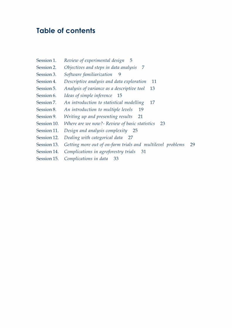
Table of contents

Session 1. Review of experimental design 5Session 2. Objectives and steps in data analysis 7Session 3. Software familiarization 9Session 4. Descriptive analysis and data exploration 11Session 5. Analysis of variance as a descriptive tool 13Session 6. Ideas of simple inference 15Session 7. An introduction to statistical modelling 17Session 8. An introduction to multiple levels 19Session 9. Writing up and presenting results 21Session 10. Where are we now?- Review of basic statistics 23Session 11. Design and analysis complexity 25Session 12. Dealing with categorical data 27Session 13. Getting more out of on-farm trials and multilevel problems 29Session 14. Complications in agroforestry trials 31Session 15. Complications in data 33

55

1. R

evie

w o

f ex

per

imen

tal d

esig

nEx

erc

ise

s

1Review of experimental designReview of experimental designReview of experimental design1Se

ssio

nSe

ssio

n

Exercise 1 - Sample protocol

The task is to study the protocol for an experiment to make sure you understand and are

able to describe the design used. Your group will be allocated one of the following trials:

a) Influence of improved fallows on soil P fractions, on-farm trial

b) Effect of Tithonia diversifolia and Lantana camara mulches on crop yields in farmers fields

c) Screening of suitable species for three-year fallow

d) Upperstorey/understorey tree management trial

You can find the protocols for these trials in Part 4 (Experiments portfolio) of the Data

analysis of agroforestry experiments workshop materials.

Start by looking at the objectives. Are these clearly stated? Can you understand them?

Do they seem to be complete?

Now look at each of the following:

treatments

measurements

layout

For each of them, try to describe clearly and exactly what was done. If it is not clear,

explain why you find it difficult - what further information would help?

Choose a group member to be the rapporteur. Prepare a brief (maximum 4 minutes!)

verbal report on the experiment you have been looking at. Highlight the four points of objectives,

treatment, measurements and layout. Do NOT spend time explaining the background or context

of the trial. You may critique the trial and suggest improvements but the main focus of the report

should be a simple description of the design used.

6

1. R

evie

w o

f ex

per

imen

tal d

esig

n

6

Exe

rcis

es

Exercise 2 - Participants protocol

Now repeat the analysis carried out in Part 1 but looking at the protocol for a trial

provided by one of your group members.

Again you are looking to see whether you can identify the objectives, treatments,

measurements and layout.

You may be critical in your analysis, but be constructive as well!

Choose a new rapporteur. Again prepare a short verbal report. You do not need to

explain all the details of the experiment. Instead concentrate on the aspects that made it hard to

understand. You do NOT have to present a revised protocol, but positive suggestions for

improvement are welcome.

7

2. O

bje

ctiv

es a

nd s

tep

s in

da

ta a

naly

sis

7

Exe

rcis

es

2Objectives and steps in data analysisObjectives and steps in data analysis2Se

ssio

nSe

ssio

n

Exercise 1 - Sample protocol

Working in your groups and using the protocol from Part 4 (Upperstorey/understorey

tree management trial) in the Experiments portfolio that you looked at in Session 1:

Work out what the objectives of the analysis should be, knowing the trial objectives and

the data available.

Describe the summaries (means, rates, etc.) that are needed to meet the analysis objectives.

Design the tables and graphs, which will present the experimental results. Sketch the

table or graph frame, add labels but don’t put in experimental data — use rough estimates

of expected data to illustrate what the graph or table might look like.

Define exactly which data will be used. For example, if yield was measured every season,

will there be separate presentations for each season? From the average across all seasons?

From some discounted cumulative total?

Prepare a short report (one or two overhead transparencies) that displays the planned

tables and graphs and discusses any difficulties encountered.

Exercise 2 - Participants protocol

Now repeat the task of Exercise 1, but using a trial protocol provided by a participant in

your group. Prepare a brief report which displays the tables and graphs planned, but also

explain any difficulties you had completing the assignment.

You can use the results of this exercise (and Exercise 2 in Session 1) to start a file for the

analysis of your own data.

2. O

bje

ctiv

es a

nd s

tep

s in

da

ta a

naly

sis

88

Exe

rcis

es

9

3. S

oft

wa

re f

am

ilia

riza

tion

9

Exe

rcis

es

3Software familiarizationSoftware familiarization3Se

ssio

nSe

ssio

n

Exercise 1 — Introduction to GenStat

Follow the Introductory Tutorial on GenStat. You will find it in Part 1 of the GenStat for

Windows Introductory Guide (GWIM). We estimate that it will take you up to one hour.

Do not spend too long on aspects that are unclear, but make a note of any points for

discussion. We will have a review at the end of this exercise where you can ask the resource

person to answer any questions you have.

Exercise 2

1. In this workshop most data are stored in Excel spreadsheets and need to be imported

into GenStat for analysis. Import the data from the trial ‘Tithonia/Lantana on-farm mulch’.

Check that the importing has worked as expected. Use the data to find the mean yield

across all the farms. Also draw a boxplot of grain yield for each treatment.

2. We have also seen how to use RESTRICT in GenStat to examine only a subset of your

data. Go to the Explanatory Analysis section of GWIM. You should find it in Part 1 of the

manual in the ‘Factors, data exploration and analysis of variance’ section. Start on the

second page of this section where it begins to use data from the ‘Tithonia/Lantana on-farm

mulch’ trial. In this example it restricts the data to look at only one of the districts

(Central). Follow the example and produce a boxplot of grain yield for each treatment,

but only for the Central district.

If you have time, use any of our other example data sets to practice the method of

restricting data. You could try to restrict by rows or by column values.

Exercise 3 — Datasets for analysis

In the initial session on Data Management we looked critically at how data can be most

accurately and efficiently stored. At the end of that session’s practical exercises you should have

reached the stage where your own files are ‘neat and tidy’. Now try to import your data into

GenStat. If it works first time, with all the data looking as expected, excellent! If not, try to

identify the problems, correct them in the spreadsheet and try again.

3. S

oft

wa

re f

am

ilia

riza

tion

1 01 0

Exe

rcis

es

GenStat hint:

An easy way of transferring data into GenStat from Excel is to ‘name’ the required

section of your data first. Within Excel highlight the data you wish to transfer, then go to the

box in the top-left of the spreadsheet, at the moment it should read the name of the first cell

you have highlighted. Within this box you can now name your highlighted section e.g. type

‘data’ into the box. When you go into GenStat and ask to import your Excel file, the item

R:‘data’ will now be shown in the list. By selecting this range your data will automatically

be read into GenStat, using the correct cell range and labelling the columns as they were

labelled in Excel.

1 1

4. D

escr

iptiv

e a

naly

sis a

nd d

ata

exp

lora

tion

1 1

Exe

rcis

es

Exercise 1 — Sample experiments

In this practical you are required to carry out some preliminary analysis of the data

collected in one of the following studies:

a) Influence of improved fallows on soil P fractions, on-farm trial

b) Effect of Tithonia diversifolia and Lantana camara mulches on crop yields in farmers fields

c) Screening of suitable species for three-year fallow

d) Upperstorey/understorey tree management trial

Choose the trial that you have discussed in your previous group discussion sessions.

Your specific tasks are as follows:

i) In Session 2 you were asked to identify at least one skeleton table or graph to use as a

sensible way of summarizing your results, which would address the objectives of the

trial. Here you are now required to extract the data to produce this (or these) table(s) or

graph(s).

ii) Consider what other questions you would like to ask about the data and identify whether

they can be addressed by a table or graph. Produce the appropriate summary, and

comment on the results.

e.g. in the ‘Effect of Tithonia diversifolia and Lantana camara mulches trial’ which some of you

have looked at, examples of questions might be ‘How many farmers in each district achieved the

target biomass application of 100 kg/plot?’ or ‘Are the treatment differences influenced by the

incidence of striga and/or streak on the plots?’

iii) Use appropriate methods to consider the variation in the data. Are there any strange

values? What can you, or should you, do about them?

You are expected to use boxplots, scatterplots, tables of sensible summary statistics

(such as the mean) and cross-tabulations. In some cases you will want to do this for the whole

dataset, and in other cases you might want to look at subsets of the data (for instance in the on-

farm trial you might wish to look at the patterns in the two districts separately).

4Descriptive analysis and data explorationDescriptive analysis and data exploration4Se

ssio

nSe

ssio

n

4. D

escr

iptiv

e a

naly

sis a

nd d

ata

exp

lora

tion

1 21 2

Exe

rcis

es

Exercise 2 — Participant experiments

[This exercise may be moved to an additional session, after Session 9 where participants can attempt a complete

analysis of their data using what they have learnt in Sessions 1 - 8].

Carry out some preliminary analyses on the dataset that you used in the second practical

in Session 2 where you looked at the analysis in relation to the objectives. This might be your

own, or someone else’s data. In that earlier practical you should have identified tables or graphs

you wanted to produce. Start there, produce them and discuss the patterns that emerge.

Then carry out further explorations using the ideas and techniques you have just learnt

in Exercise 1 in this session.

GenStat hints:

From the Stats pull-down menu

From Summary Statistics

Choose Summaries of Groups : for tables

At the Spread pull-down menu

Choose Restrictions

And Using factor levels… : to work with a subset of the data

Unrestrict Unselected Levels : to remove the restriction

From the Graphics pull-down menu

Boxplots… : for graphical summaries

Pointplots …

If you are using graphics and you want to keep several graphics windows open at once,

then when you have the GenStat Graphics window open, click on Multiple Windows at the

Options pull-down menu.

Refer to the GWIM for more detail on the commands you need.

1 3

5. A

naly

sis o

f va

rianc

e a

s a

des

crip

tive

tool

1 3

Exe

rcis

es

5Analysis of variance as a descriptive toolAnalysis of variance as a descriptive tool5Se

ssio

nSe

ssio

n

Exercise 1 — Understanding ANOVA

The first exercise aims at reviewing your understanding of the role of the ANalyses Of

VAriance (ANOVA) table and to practice producing an ANOVA for a range of simple designs.

GWIM is used for this purpose. This should not take more than 30 minutes.

1. Read into GenStat the data from the ‘Screening of suitable species for three-year fallow’

trial (‘Fallow N.xls’). Restrict the data to include only the 1992 season of data (you should

have already learnt how to restrict your data sets). Note that this trial has a Randomized

Complete Block Design with 10 treatments and 4 replicates. Do an ANOVA with grain

yield as your response, setting the options so that F-probabilities and standard errors

are not given. Check that you understand all of the output.

2. In the lecture we described the analysis of the 2-factor ‘Upperstorey/understorey tree

management’ trial. Repeat the analysis (again without F-probabilities and standard

errors). Check that you understand all of the output. (N.B. Read into GenStat the data

from the sheet R:fact – this contains the altered structure data)

3. In the data from the example above, change some of the values to simulate possible entry

errors. For example density = 0 and Under = No; change Block 1 observation to 22.5, and

Block 3 to 22.1. Why is the odd residual pointed out by GenStat not one of the ones that

were changed?

4. With the original data restored, give the plot of the treatment factors, as we did in the

lecture. Also give the breakdown of the treatment term into the polynomial effects as

shown in the lecture.

(Hint: type or use the <Contrasts> button to change the treatment term from

density*under to Pol(density; 1)*under.)

5. A

naly

sis o

f va

rianc

e a

s a

des

crip

tive

tool

1 41 4

Exe

rcis

es

Exercise 2 — Participant experiments

Take one of the datasets that you used for the descriptive statistics in the last session and

conduct an ANOVA on this set. Does it add anything of value to the presentation that you did

then? In your discussion include at least the three following points:

1. Are there any odd or curious values? If so, then does it affect the analysis much if they are

omitted? If not, then what would you conclude? If so, then what would you do?

2. Does the analysis help in identifying which tables of means to investigate in more detail?

Also, does it tell you roughly how much importance to attach to the different levels of

each treatment factor?

3. Are you satisfied with the amount of residual variation in your trial? Is it small enough

that the objectives of the trial can be realized?

4. If the residual variation is large, can you think of ways that it can be reduced? Remember

that the basic idea is that your data = pattern + residual. So can you think of any part of

the residual that can be explained by some effects that are not included yet? Then they

could become part of the pattern and the residual would be reduced.

1 51 5

6. Id

eas

of s

imp

le in

fere

nce

Exe

rcis

es

6Ideas of simple inferenceIdeas of simple inference6Se

ssio

nSe

ssio

n

Exercise 1

In the first part of this practical we review and extend the analysis that was covered in

the lecture. Use the same set of data, namely the Kenyan on-farm experiment ‘Effect of Tithonia

diversifolia and Lantana camara mulches on crop yields in farmers fields’. Start by restricting

attention to the second district, namely West.

Repeat the ANOVA and check you understand all the output. How do the results compare

with those given in the lecture for the Central district?

In the lecture, two observations in the West district seemed odd. Try the analysis without

these observations. How do the results change?

Do the results seem valid? GenStat offers a range of residual plots to investigate this

aspect.

For the objectives of this trial it would be sensible to look at two treatment ‘contrasts’,

i.e. Lantana vs Control, and Tithonia vs Control. The lecture you have heard for Session 6 has

explained the theory behind these comparisons. Now you should try to work out the contrasts

using GenStat. In GWIM Part 2 - Analysis of Variance - Further Topics, you should find a section

entitled ‘User Defined Contrasts’ which considers the use of contrasts for a similar problem that

also has 3 treatments. Do you find it easy to use contrasts? Does it clarify the interpretation of

the results? What do you conclude in this case?

Repeat the analysis, including the contrasts on the data from the two districts together.

Start by trying to reproduce the tables shown in Part 2 - Lecture notes, page 57, Table 2. Then

add the contrasts to the analysis. Are the results clearer for the overall analysis with the 2

districts, or is it simpler to analyse the data from each district separately? Justify your approach.

1 6

6. Id

eas

of s

imp

le in

fere

nce

1 6

Exe

rcis

es

Exercise 2

Choose a different example, either from those provided, or use your own data if it is

suitable and conduct an Analysis of Variance.

You should now be able to understand all elements of the general summary that is

provided as a routine. This consists of the analysis of variance table, the table(s) of means and

the corresponding standard errors. Check that everything is understood and give an overall

summary of the results.

Now return to the protocol and assess the extent to which this overall analysis provides

answers to the objectives of the study. You are likely to find that it provides partial answers.

Reasons that the answers are not complete include:

Some different variables need to be analysed.

Some additional variables need to be included in the analysis that you have done.

There is too much unexplained variability.

There are some odd observations.

The analysis is too general; it helps, but does not answer the specific objectives.

What is the situation in your example?

What are the next steps in your analysis? Specify these and attempt them.

1 7

7. A

n in

tro

duc

tion

to s

tatis

tica

l mo

del

ling

1 7

Exe

rcis

es

7An introduction to statistical modellingAn introduction to statistical modelling7Se

ssio

nSe

ssio

n

Part 1

Review the fitting and interpretation of simple linear regression models by working

through the GWIM example on pages 61-64.

Now look again at the data from the trial ‘Screening of suitable species for three-year

fallow’. Investigate the relationship between soil inorganic N and maize yield in the second

experiment (1992). Is there any indication of a relationship? Is it a straight-line relationship? If

so, obtain estimates of the slope and intercept of the line. Assess the quality of the fit of the line

and interpret the model.

Part 2

Use the regression commands in GenStat to produce an analysis of variance table,

treatment mean estimates and s.e.d.’s for an example that you can also analyse with the ANOVA

commands. A good example would be the second experiment in ‘Screening of suitable species for

three-year fallow’, which you’ve used in Part 1. Confirm that you get the same results using the

two approaches.

Now carry out an analysis to identify treatment effects for an experiment that can not be

analysed simply using the ANOVA commands, because block or treatment factors, are non-

orthogonal or unbalanced. A good example is the ‘Fertilizer, Tithonia and Lantana mulch as sources

of phosphorus for maize’ trial (look in Part 4 of the course booklets to find the protocol), or you

may have one of your own.

Carry out an exploratory analysis then carry out an ANOVA that reveals the importance

of block and treatment effects. Finally estimate treatment means that are adjusted for any possible

block effects and interpret them.

7. A

n in

tro

duc

tion

to s

tatis

tica

l mo

del

ling

1 81 8

Exe

rcis

es

Part 3

Now return to the example ‘Screening of suitable species for three-year fallow’. Try to

answer the following questions:

1. We saw that in Experiment 1 there was still considerable difference in yield between

treatments after allowing for effects of inorganic N. Can these differences be attributed

to either the aerobic mineralizable N (AEROBIC) or the striga count (STRIGA)?

2. Are the effects of inorganic N on yield the same for both Experiments 1 and 2?

1 9

8. A

n in

tro

duc

tion

to m

ultip

le le

vels

1 9

Exe

rcis

es

8An introduction to multiple levelsAn introduction to multiple levels8Se

ssio

nSe

ssio

n

Exercise 1

In this practical, working in pairs, repeat the analysis of the split-plot example, ‘Influence

of improved fallows on soil P fractions’ on-farm trial, which was discussed in the lecture.

The objective here is to understand how to request the correct analysis from the software

as well as to understand the output.

Exercise 2

(a) Inspect the data from the ‘Effect of Tithonia diversifolia and Lantana camara mulches on crop

yields in farmers fields’ trial to assess its structure in terms of how many different levels

there are and what measurements were made at each level. Produce some tabulations of

these factors and identify, but do not carry out, some simple analyses which could be

performed.

A short discussion of this will follow.

(b) Work through the exercise on ‘multiple observations per experimental unit’, which is in

GWIM Part 2 – Analysis of Variance – Further Topics. The objective is to learn the

necessary computing steps needed to be able to carry out a satisfactory analysis when

there are multiple observations per experimental unit.

(c) Use the ‘Leucaena trichandra seed production trial’ data, which was discussed in the lecture

to try out some of the different approaches we can use to deal with multiple levels. You

should also analyse the data as (i) a randomized complete block design with replicate

and family effects and (ii) as an incomplete block design with 100 blocks of 4 plots.

A short discussion of both of these will follow, summarizing the main points, which

emerged in (c).

8. A

n in

tro

duc

tion

to m

ultip

le le

vels

2 02 0

Exe

rcis

es

2 1

9. W

ritin

g u

p a

nd p

rese

ntin

g r

esul

ts

2 1

Exe

rcis

es

9Writing up and presenting resultsWriting up and presenting results9Se

ssio

nSe

ssio

n

The Challenge

During the course you have been analysing data from a number of different studies,

provided by the course organizers, brought by you or brought by another participant.

Now we challenge you to:

Take one objective from a study you have been working on.

Carry out the statistical analysis to meet the objective.

Present the results using a single graph or table and a single paragraph of text.

Prepare the output in two ways:

1. A single printed page, which can be given to various people to comment on.

2. A single transparency with the table or graph together with a 100 word (maximum)

commentary that you can present to the whole group.

The aim of this challenge is to force you to think about the most effective and concise way

of describing the results. The reports have to be complete, presenting all the information necessary

to meet the objective but cannot include anything unnecessary. It is not necessary to include any

of the background or methods used in the study.

Ask for help, from resource persons, when selecting a study and objective for this

challenge.

9. W

ritin

g u

p a

nd p

rese

ntin

g r

esul

ts

2 22 2

Exe

rcis

es

2 32 3

10. W

here

are

we

now

?- R

evie

w o

f b

asic

sta

tistic

sEx

erc

ise

s

10Where are we now?- Review of basic statisticsWhere are we now?- Review of basic statistics10Se

ssio

nSe

ssio

n

Review and presentation

You have been put into a group and the group has been given a topic from the course

so far.

Now you are asked to prepare a brief review of that topic. The review should summarize

the key points on the topic and the importance of it to your work.

The review should be in the form of a presentation taking no more than 5 minutes and

using less than 5 slides.

Each group should also provide a discussant, who adds a 2 minute discussion to the

review. The discussant should concentrate on the problems they faced with the topic, the extent

to which these have been overcome and the confidence they now feel in the area.

2 4

10. W

here

are

we

now

?- R

evie

w o

f b

asic

sta

tistic

s

2 4

Exe

rcis

es

2 52 5

11. D

esig

n a

nd a

naly

sis c

omp

lexi

tyEx

erc

ise

s

11Design and analysis complexityDesign and analysis complexity11Se

ssio

nSe

ssio

n

Exercise 1

Working in pairs:

a) Carry out an analysis of non-normal data using the example in GWIM pages 154 - 156.

b) Investigate the idea of exploring treatment structure further using the example in GWIM,

pages 122 - 125.

Exercise 2

Work in groups looking at either one of:

a) Explore the ideas of complex treatment structure further by analysing the data from

‘Upperstorey/understorey tree management trial’.

b) Carry out an analysis of the proportion of trees surviving in October in the trial ‘Fruit

trees survival’.

Try to:

i) Discuss the complexity of the problem and decide how it can be addressed.

ii) Attempt an appropriate analysis and interpret the findings.

You will probably need help using GenStat. Before asking for that help try to work out

exactly what you are trying to achieve with the analysis. Try to use the resource people as

‘GenStat experts who know no statistics’!

2 6

11. D

esig

n a

nd a

naly

sis c

omp

lexi

ty

2 6

Exe

rcis

es

Prepare a short presentation that covers:

the nature of any complexity

the strategy for coping with it

the analysis and interpretation.

2 72 7

12. D

ealin

g w

ith c

ate

go

rica

l da

taEx

erc

ise

s

12Dealing with categorical dataDealing with categorical data12Se

ssio

nSe

ssio

n

Exercise

1. In the lecture, data from ‘Improved fallows and rock phosphate: farmers’ experiences’

were analysed, focusing on the response variable PresIF99, which records whether an

improved fallow was present in 1999. Repeat the analyses using the 1997 and 1998

variables (PresIF97 and PresIF98) and determine whether the influence of ethnicity,

practicing of natural fallow and farm size are much the same in the earlier years.

2. In the lecture separate analyses were carried out to look at the effects of categorical

explanatory variables (ethnicity and natural fallow) and the continuous variable

farmsize. Try to complete and interpret an analysis that considers all three in the same

model.

3. Look carefully at the protocol ‘Fruit trees survival’ and the associated data set. A number

of trees of several species were planted on each farm. The planting niche was chosen as

either shallow or deep soil and chicken manure was applied to some of the trees. The

objectives of the analysis are to determine how chicken manure and planting affect

survival of these species. You will have to think carefully about if and how to allow for

the different farms and species in the study. You might also experience some new technical

problems in fitting models. Try to understand their source and think of solutions.

2 8

12. D

ealin

g w

ith c

ate

go

rica

l da

ta

2 8

Exe

rcis

es

2 92 9

13. G

ettin

g m

ore

out

of

on-

farm

tria

ls a

nd m

ultil

evel

pro

ble

ms

Exe

rcis

es

1313Se

ssio

nSe

ssio

nGetting more out of on-farm trials

and multilevel problemsGetting more out of on-farm trials

and multilevel problems

Exercise

Use the data from the Malawi on-farm trial, ‘On farm cropping with Sesbania and Gliricidia’.

Consider the following objectives, all of which refer to the ‘98 season, when the rainfall was

reasonable and it is expected that trees will have had time to become well established.

1. How much does inclusion of trees (either Gliricidia or Sesbania) increase yield compared to

a crop-only control, and how much does this vary across farms?

2. It is expected that the trees will be most effective when soil P is high (the trees add N to

the system but not P). Is this the case?

3. The steeper sloping fields tend to have shallow soil and are subject to erosion. We would

not expect the trees to have much effect there. Is there evidence for that?

4. We might also expect that the steeper fields, being generally less productive, are often left

unweeded. What is the evidence for that?

For each of these:

a) Carry out an exploratory or descriptive analysis that answers the question.

b) Determine the level (within or between farms) at which the relevant information occurs.

c) Carry out an inferential analysis if you are able to.

d) If you are unable, describe the analysis you would like to carry out and why it is difficult.

3 0

13. G

ettin

g m

ore

out

of

on-

farm

tria

ls a

nd m

ultil

evel

pro

ble

ms

3 0

Exe

rcis

es

3 1

14.

Co

mp

lica

tions

in a

gro

fore

stry

tria

ls

3 1

Exe

rcis

es

14Complications in agroforestry trialsComplications in agroforestry trials14Se

ssio

nSe

ssio

n

Exercise

Choose to work on either a problem with repeated measures in space or in time (you will

not have time for both!).

If interested in the spatial problem, work on the RAC trial. Try to repeat the analyses

done in the lecture, but using grain yield rather than biomass. Then look carefully at the summary

graphs and decide if there are other summary statistics it would be informative to analyse.

Carry out such an analysis.

If interested in repeated measures in time have a look at ‘Prototype hedgerow

intercropping systems’. Look at the objectives and try to meet them. You will need to start by

producing simple graphs of the response of treatments through time, and in relation to rainfall.

The choose useful summaries and analyse them.

In both cases produce a brief presentation that describes not just the results, but any

difficulties you had producing them or understanding them.

14.

Co

mp

lica

tions

in a

gro

fore

stry

tria

lsEx

erc

ise

s

3 23 2

3 3

15.

Co

mp

lica

tions

in d

ata

3 3

Exe

rcis

es

15Complications in dataComplications in data15Se

ssio

nSe

ssio

n

Exercise

This practical is best done with sets of data brought by participants. Where this is not

possible, the agroforestry datasets can be used instead.

Participants, in small groups should take one or more problems from the table given in

the lecture that corresponds with a complication in the dataset they have. They should then

investigate possible solutions to that problem, which are to be described in the discussion

session.

The groups should check that they are each investigating different problems.

For guidance on the types of solution, reference should be made to supporting documentation.

This includes:

The lecture note for this session.

The GWIM guide, particularly the section entitled Analysis of Variance - Further Topics.

MCH, particularly Chapter 8.

Where possible participants should try different solutions to the complication, so that

these can be compared.

Each group should prepare a short presentation. These presentations are to describe the

method(s) of resolving the complication to the whole group. They are not to discuss the data

analysis itself.

The presentations should also discuss reference material that helped in the solution.