PDF - 216K - Air Resources Board - State of California
272
CALIFORNIA ENVIRONMENTAL PROTECTION AGENCY AIR RESOURCES BOARD STAFF REPORT: INITIAL STATEMENT OF REASONS FOR PROPOSED RULEMAKING, PUBLIC HEARING TO CONSIDER THE “LEV III” AMENDMENTS TO THE CALIFORNIA GREENHOUSE GAS AND CRITERIA POLLUTANT EXHAUST AND EVAPORATIVE EMISSION STANDARDS AND TEST PROCEDURES AND TO THE ON-BOARD DIAGNOSTIC SYSTEM REQUIREMENTS FOR PASSENGER CARS, LIGHT-DUTY TRUCKS, AND MEDIUM-DUTY VEHICLES, AND TO THE EVAPORATIVE EMISSION REQUIREMENTS FOR HEAVY-DUTY VEHICLES This report has been reviewed by the staff of the California Air Resources Board and approved for publication. Approval does not signify that the contents necessarily reflect the views and policies of the Air Resources Board, nor does the mention of trade names or commercial products constitute endorsement or recommendation for use. Date of Release: December 7, 2011 Scheduled for Consideration: January 26, 2012
Transcript of PDF - 216K - Air Resources Board - State of California

CALIFORNIA ENVIRONMENTAL PROTECTION AGENCY AIR RESOURCES BOARD
STAFF REPORT: INITIAL STATEMENT OF REASONS FOR PROPOSED RULEMAKING, PUBLIC
HEARING TO CONSIDER THE “LEV III” AMENDMENTS TO THE CALIFORNIA GREENHOUSE GAS AND CRITERIA POLLUTANT EXHAUST AND EVAPORATIVE
EMISSION STANDARDS AND TEST PROCEDURES AND TO THE ON-BOARD DIAGNOSTIC SYSTEM REQUIREMENTS FOR PASSENGER CARS, LIGHT-DUTY
TRUCKS, AND MEDIUM-DUTY VEHICLES, AND TO THE EVAPORATIVE EMISSION REQUIREMENTS FOR HEAVY-DUTY VEHICLES
This report has been reviewed by the staff of the California Air Resources Board and approved for publication. Approval does not signify that the contents necessarily reflect the views and policies of the Air Resources Board, nor does the mention of trade names or commercial products constitute endorsement or recommendation for use.
Date of Release: December 7, 2011 Scheduled for Consideration: January 26, 2012

Page ES-1
EXECUTIVE SUMMARY Background Despite significant progress in reducing smog-forming and particulate matter criteria emissions from the passenger vehicle fleet, California needs further reductions in order to meet State and federal ambient air quality standards. In addition, climate change continues to pose a serious threat to the economic well-being, public health, natural resources, and environment of California. To address the challenge presented by climate change, vehicle greenhouse gas (GHG) emissions must be drastically reduced to meet our goal of an 80% reduction from 1990 levels by 2050. California’s Light-Duty Vehicle Program Criteria Emissions In 1990, the Air Resources Board (ARB or Board) established the Low Emission Vehicle (LEV) program that contained the most stringent exhaust emission regulations ever for light-duty passenger cars and trucks. The regulations included three primary elements: (1) tiers of increasingly stringent exhaust emission standards, (2) a fleet-average emission requirement for 1994-2003 that required manufacturers to phase-in a progressively cleaner mix of vehicles from year to year, and (3) a requirement that a specified percentage of passenger cars and lighter light-duty trucks be zero emission vehicles (ZEVs), vehicles with zero emissions of any pollutants. In 1999, ARB adopted the second phase of the LEV program. These amendments, known as LEV II, set more stringent fleet average non-methane organic gas (NMOG) requirements for model years 2004-2010 for passenger cars and light-duty trucks and established a new more stringent super ultra-low emission vehicle (SULEV) standard. In addition, a partial zero-emission vehicle (PZEV) category was established for vehicles meeting the SULEV emission standard that also included extended 150,000-mile durability, zero fuel evaporative emissions, and extended emission warranty requirements. PZEVs could be used to meet a portion of the zero-emission vehicle requirement. The amendments also expanded the light-duty truck category to include trucks and SUVs up to 8,500 lbs. gross vehicle weight rating (GVWR) and required these vehicles to meet the same emission standards as passenger cars, and extended full useful life from 100,000 miles to 120,000 miles. The LEV II amendments also established more stringent emission standards for medium-duty vehicles (MDVs) between 8,501-14,000 lbs. GVW. Greenhouse Gas Emissions Recognizing the increasing threat of climate change to the well-being of California’s citizens and the environment, in 2002 the legislature adopted and the Governor signed AB 1493 (Chapter 200, Statutes 2002, Pavley). AB 1493 directed ARB to adopt the maximum feasible and cost-effective reductions in GHG emissions from light-duty vehicles. Vehicle GHG emissions included carbon dioxide (CO2), methane (CH4), and nitrous oxide (N2O) that are emitted from the tailpipe, as well as emissions of HFC134a,

Page ES-2
the refrigerant currently used in most vehicle air conditioning systems. Table ES-1 below lists the global warming potential of these GHGs. Table ES-1. Numerical Estimates Of Global Warming Potentials Compared With CO2 (Kilograms Of Gas Per Kilogram Of CO2 -- Adapted From IPCC 2007c1)
Climate
Pollutants Lifetime (years)
Global Warming Potential 20 years 100 years 500 years
CO2 ~150 1 1 1 CH4 12 72 25 7.6 N2O 114 289 298 153
HFC134a 14 3830 1300 435 As directed by AB 1493, ARB adopted what is commonly referred to as the Pavley regulations, the first in the nation to require significant reductions of GHGs from motor vehicles. These regulations, covering the 2009-2016 and later model years, call for a 17% overall reduction in climate change emissions from the light-duty fleet by 2020 and a 25% overall reduction by 2030. They also formed the foundation for the federal GHG program for light-duty vehicles for 2012-2016 model years. After the Board adopted the Pavley regulations, the legislature adopted and the Governor signed AB 32, the California Global Warming Solutions Act (Chapter 488, Statutes 2006, Nuñez/Pavley). AB 32 charges ARB with the responsibility of monitoring and regulating GHG emissions in the State. AB 32 also directed ARB to prepare a Scoping Plan outlining the State’s strategy to achieve the maximum feasible and cost-effective reductions in furtherance of reducing GHG emissions to 1990 levels by 2020. Measure T1 of the Scoping Plan anticipates an additional 3.8 million metric tons carbon dioxide equivalent (MMTCO2e) reduction by 2020 beyond the reductions from the 2009-2016 AB 1493 standards. In addition, in 2005, in order to mitigate the long-term impacts of climate change, the Governor issued Executive Order S-3-05. Among other actions, the Executive Order called for reducing GHG emissions to 80 percent below 1990 levels by 2050. This ambitious yet achievable reduction path and goal are considered necessary to stabilize the long-term climate. ZEV Program Although originally part of the LEV program, in 1999, in recognition of the increasing maturity of zero emission technologies and the critical role they can play in achieving California’s air quality goals, ARB established the ZEV program as a stand-alone one. Since then, the program has been modified several times to address the pace of development of zero emission technologies.
1 IPCC 2007c: Working Group I: The Physical Science Basis, Chapter 2: Changes in Atmospheric Constituents and in Radiative Forcing, available at http://www.ipcc.ch/pdf/assessment-report/ar4/wg1/ar4-wg1-chapter2.pdf

Page ES-3
At its March 2008 hearing, the Board directed staff to redesign the 2015 and later model year ZEV program by strengthening the requirement and focusing primarily on zero emission technologies – battery electric vehicles, hydrogen fuel cell vehicles, and plug-in hybrid electric vehicles – in order to ensure that these low GHG technology vehicles transition from the demonstration phase to full commercialization in a reasonable timeframe. The resulting proposed amendments to the ZEV program are presented in a separate staff report, also part of this comprehensive vehicle rulemaking package, the Advanced Clean Cars program. Advanced Clean Cars Program Continuing its leadership role in the development of innovative and ground breaking emission control programs and to achieve California’s goals of meeting ambient air quality standards and reducing climate changing GHG emissions, ARB staff has developed the Advanced Clean Cars (ACC) program. The Advanced Clean Cars program combines the control of smog-causing pollutants and greenhouse gas emissions into a single coordinated package of requirements for model years 2015 through 2025 and assures the development of environmentally superior cars that will continue to deliver the performance, utility, and safety vehicle owners have come to expect. The ZEV program will act as the focused technology-forcing piece of the Advanced Clean Cars program by requiring manufacturers to produce increasing numbers of pure ZEVs and plug-in hybrid electric vehicles in the 2018-2025 model years. In addition, the Advanced Clean Cars program includes amendments to the Clean Fuels Outlet regulation that will assure ultra-clean fuels such as hydrogen are available to meet vehicle demands brought on by these amendments to the ZEV program. Beyond 2025, the dominant force for lowering emissions from vehicles in California will be climate change. In order to meet our 2050 GHG goal, the new vehicle feet will need to be primarily composed of advanced technology vehicles such as electric and fuel cell vehicles by 2035 in order to have nearly an entire new and used advanced technology fleet by 2050. Accordingly, the Advanced Clean Cars program coordinates the goals of the LEV, ZEV, and Clean Fuels Outlet programs in order to lay the foundation for the commercialization and support of these ultra-clean vehicles. Figure ES-1 shows the cumulative on-road passenger vehicle fleet mix for one scenario developed by staff that achieves California’s 2050 GHG emission reduction goal. Importantly, ZEV sales must constitute nearly 100% of new vehicles in 2040 for ZEVs to constitute approximately 87% of the on-road fleet by 2050.

Page ES-4
Figure ES-1. On Road Light-Duty Vehicle Scenario to Reach 2050 Goal
Criteria Emission Standards and New Certification Fuel Requirements In order to achieve further criteria emission reductions from the passenger vehicle fleet, staff is proposing several amendments representing a significant strengthening of the LEV program. The major elements of the proposed LEV III program are:
• A reduction of fleet average emissions of new passenger cars (PCs), light-duty trucks (LDTs) and medium-duty passenger vehicles (MDPVs) to super ultra-low-emission vehicle (SULEV) levels by 2025;
• Replacement of separate NMOG and oxides of nitrogen (NOx) standards with combined NMOG plus NOx standards, which provides automobile manufacturers with additional flexibility in meeting the new stringent standards;
• An increase of full useful life durability requirements from 120,000 miles to 150,000 miles, which guarantees vehicles operate longer at these extremely low emission levels;
• A backstop to assure continued production of super-ultra-low-emission vehicles after PZEVs as a category are moved from the Zero-Emission Vehicle program to the LEV program in 2018;
• More stringent particulate matter (PM) standards for light- and medium-duty vehicles, which will reduce the health effects and premature deaths associated with these emissions;

Page ES-5
• Zero fuel evaporative emission standards for PCs and LDTs, and more stringent evaporative standards for medium- and heavy-duty vehicles (MDVs);
• More stringent supplemental federal test procedure (SFTP) standards for PC and LDTs, which reflect more aggressive real world driving and, for the first time, require MDVs to meet SFTP standards.
Table ES-2 below lists the proposed fleet average NMOG plus NOx requirements for PCs, LDTs, and MDPVs for model years 2015-2025.
Table ES-2. Fleet Average NMOG Plus NOx Exhaust Emission Requirements for Light-Duty Vehicles (150,000 mile Durability Basis)
Model Year Fleet Average NMOG plus NOx
(grams per mile) All PCs; LDT1s LDT2s; MDPV
2015 0.100 0.119 2016 0.093 0.110 2017 0.086 0.101 2018 0.079 0.092 2019 0.072 0.083 2020 0.065 0.074 2021 0.058 0.065 2022 0.051 0.056 2023 0.044 0.047 2024 0.037 0.038 2025 0.030 0.030
Staff is also proposing three additional light-duty vehicle emission standards (ULEV70, ULEV50, and SULEV20) to which manufacturers may certify their vehicles when meeting the fleet average emission requirement. The numerical part of the standard category, such as 20 in SULEV20, refers to the emission standard, in thousandths of a gram per mile. Combined with an extended fleet average emission requirement phase-in period, providing these additional emission standards will allow manufacturers to phase-in additional emission componentry across their fleet in a cost-effective manner. Current California certification gasoline contains methyl tertiary butyl ether (MTBE) as an oxygenate, reflecting commercial gasoline sold prior to 2003 and as such does not represent gasoline currently sold in California, which does not contain MTBE. The current maximum ethanol content allowed in commercial gasoline is 10 percent by volume and is expected to remain at 10 percent for the foreseeable future. Accordingly, staff is proposing to change the certification fuel specifications to be more representative of current in-use fuel. Staff is also proposing that vehicles certify on a fuel that reflects the octane requirement that they are operated on in-use. Therefore, for vehicles that consumers must operate on premium fuel to maintain warranty coverage,

Page ES-6
manufacturers may certify on premium grade fuel, while all others must certify on regular grade fuel. Greenhouse Gas Emission Standards The proposed GHG emission standards would reduce new passenger vehicle carbon dioxide (CO2) emissions from their model year 2016 levels by approximately 34% by model year 2025, from about 251 to about 166 gCO2/mile, based on the projected mix of vehicles sold in California. The basic structure of the standards includes two categories – passenger cars and light-duty trucks – that are consistent with federal categories for light-duty vehicles. The standard targets would reduce car CO2 emissions by about 36% and truck CO2 emissions by about 32% from model year 2016 through 2025. Figure ES-2 illustrates the basic target emission trends that are projected from the car and truck standards. For the 2017-2025 model year standards, ARB proposes to use the United States Environmental Protection Agency (USEPA) approach and adopt separate standards for CO2, CH4, and N2O. Figure ES-2. Target Emission Reductions from GHG Standards
Table ES-3 shows the year-by-year new vehicle CO2 reductions that are projected as a result of the standards from cars, light-duty trucks, and combined light-duty vehicles. The projected result overall from 2016-2025 from these standards is to reduce car CO2 emissions by approximately 4.9%/year, reduce truck CO2 emissions by approximately 4.1%/year, and reduce combined light-duty CO2 emissions by approximately 4.5%/year from 2016 through 2025. These CO2 emission reduction estimations are approximate because the required emission level to achieve compliance with the standards for each vehicle manufacturer depends on their ultimate sales mix of vehicles.

Page ES-7
Table ES-3. Projected Targets for Light-Duty Vehicle gCO2/mile Emission Rates
Model Car Truck Combined light-duty
year gCO2/mi Annual
change gCO2/mi Annual change gCO2/mi Annual
change Baseline 2008 291 396 336
Previous Rule Targets
2013 256 2.8% 330 2.8% 283 2.6% 2014 248 3.3% 321 2.8% 275 2.8% 2015 236 4.5% 306 4.5% 263 4.3% 2016 226 4.5% 292 4.5% 251 4.4%
Proposed Rulemaking Targets
2017 213 5.5% 290 0.7% 243 3.2% 2018 203 4.9% 280 3.5% 233 4.2% 2019 192 5.2% 273 2.8% 224 4.0% 2020 183 4.9% 264 3.0% 215 3.9% 2021 173 5.5% 245 7.5% 201 6.3% 2022 165 4.4% 233 4.9% 192 4.6% 2023 158 4.5% 221 4.9% 183 4.8% 2024 151 4.5% 210 5.0% 174 4.8% 2025 144 4.6% 200 4.9% 166 4.8%
Average change, (2016-2025) 4.9% 4.1% 4.5% Change, 2008-2016 -23% -26% -25% Change, 2016-2025 -36% -32% -34% Change, 2008-2025 -51% -50% -51%
Notes: Car, truck, overall targets shown are based on projected sales of vehicles by footprint, category (ultimate gCO2/mile levels are determined by end-of-year sales); the original California GHG standards for model years 2009-2011 are based on a different two-category system (PC/LDT1 and LDT2) than the car and truck system of the 2012-2016 federal standards and proposed 2017-2025 standards; Difference of individual columns may not match due to rounding.
The already low CH4 and N2O standards will reflect the same stringency as the prior GHG standards. The net result is that, like the current 2009-2016 California GHG standards, the proposed 2017-2025 standards account for all major sources of vehicle GHG emissions, including upstream emissions associated with vehicle fuels. In addition, California is proposing to align its vehicle air conditioning system requirements with federal requirements. Maximum Feasible and Cost-Effective Technologies Vehicle manufacturers need sufficient lead-time to implement new technologies across their vehicle lines both from a feasibility and cost-effectiveness standpoint. Manufacturers will be resource challenged over the next 15 years as they strive to develop and implement technologies ranging from advanced gasoline and diesel engines to electric and fuel cell vehicles, while at the same time lowering criteria emissions of their combustion engines. The phase-in of the Advanced Clean Cars program requirements recognizes this by providing manufacturers with significant lead-time and considerable compliance flexibility. Criteria Emissions The technology for controlling vehicle emissions is well understood and manufacturers have a wide range of emission control technologies available to achieve SULEV emissions. Many of these technologies are already being used today on vehicles

Page ES-8
meeting LEV II requirements and staff anticipates that with ongoing improvements to the effectiveness of these technologies, particularly catalyst technology, manufacturers will be able to meet the proposed LEV III requirements. For some vehicles, specifically the heavier vehicles with larger displacement engines, additional emission control componentry such as secondary air and hydrocarbon adsorbers may be required to achieve the proposed emission levels. Greenhouse Gas Emissions The proposed GHG standards are also predicated on many existing and emerging technologies that increase engine and transmission efficiency, reduce vehicle energy loads, improve auxiliary and accessory efficiency, and that recognize increasingly electrified vehicle subsystems with hybrid and electric drivetrains. The previous rulemakings (i.e., California’s 2009-2016 and federal 2012-2016 standards) established an original technical basis for the proposed GHG standards. This rulemaking builds on this existing technical foundation with new technical data and understanding of evolving state-of-the-art engine, transmission, hybrid, and electric-drive technologies. As part of this effort, and without conceding any of California’s separate authority, staff has been working with the USEPA and the National Highway Transportation Safety Administration (NHTSA) since early last year to develop a unified national GHG program for motor vehicles beyond 2016 that will also meet California’s GHG goals. Environmental Impacts Criteria Emissions Table ES-4, Table ES-5, and Table ES-6 provide the emission benefits for calendar years 2023, 2025, and 2035 for reactive organic gas (ROG), oxides of nitrogen (NOx), and particulate matter (PM2.5) respectively. Emission benefits are nearly fully realized in the 2035-2040 timeframe when most vehicles operating in the fleet are expected to be compliant with the proposed Advanced Clean Car standards. By 2035 ROG statewide emissions would be reduced by an additional 34 percent, NOx emissions by an additional 37 percent, and PM2.5 emissions by 10 percent. Table ES-4. Statewide and Regional Emission Benefits of the Advanced Clean Car Program: Reactive Organic Gas (ROG)
Statewide ROG (tons/day)
Calendar Year
Adjusted Baseline with
Rebound
Proposed Regulation with
Rebound Benefits Percent
Reduction
2023 189.6 182.9 6.6 3% 2025 175.5 164.4 11.1 6% 2035 141.1 93.6 47.4 34%

Page ES-9
Table ES-5. Statewide Emission Benefits of the Advanced Clean Car Program: Oxides of Nitrogen (NOx)
Statewide NOx (tons/day)
Calendar Year
Adjusted Baseline with
Rebound
Proposed Regulation
with Rebound Benefits Percent
Reduction
2023 201.3 185.6 15.7 8% 2025 183.6 161.2 22.4 12% 2035 136.8 86.4 50.4 37%
Table ES-6. Statewide and Regional Emission Benefits of the Advanced Clean Car Program: Particulate Matter (PM2.5)
Statewide PM2.5 (tons/day)
Calendar Year
Adjusted Baseline with
Rebound
Proposed Regulation
with Rebound Benefits Percent
Reduction
2023 26.7 26.0 0.6 2% 2025 27.2 26.3 0.9 3% 2035 29.7 26.8 2.9 10%
Staff used EMFAC 2011 to estimate the environmental benefits of the Advanced Clean Cars program. Staff’s analysis concluded that because the operating costs of vehicles meeting the GHG standards will decrease, vehicle use may increase. This effect is known as the rebound effect. When rebound rates were included in the inventory, there were negligibly (approximately one percent) fewer emission reductions compared to the substantial overall emission reductions expected from the Advanced Clean Car regulations package. Greenhouse Gas Emissions The Advanced Clean Cars program would provide major reductions in greenhouse gas emissions. Table ES-7 shows the greenhouse gas emission benefits in 2020, 2025, 2035, and 2050. By 2025, CO2 equivalent emissions would be reduced by almost 14 Million Metric Tons (MMT) per year, which is 12 percent from baseline levels. The reduction increases in 2035 to 32 MMT/Year, a 27 percent reduction from baseline levels. By 2050, the proposed regulation will reduce emissions by more than 42 MMT/Year, a reduction of 33 percent from baseline levels. Viewed cumulatively from 2017 through 2050, the proposed Advanced Clean Cars regulation would reduce emissions by more than 870 MMT CO2 Equivalent.

Page ES-10
Table ES-7. CO2-Equivalent (CO2e) Emission Benefits from Advanced Clean Car Regulations
Statewide CO2e Emissions (Million Metric Tons / Year)
Calendar Year
Adjusted Baseline with
Rebound
Proposed Regulation with
Rebound Benefits Percent
Reduction
2020 111.2 108.1 3.1 3% 2025 109.9 96.3 13.7 12% 2035 114.8 83.2 31.5 27% 2050 131.0 88.3 42.7 33%
Cost Effectiveness Criteria Emissions Staff based its cost-effectiveness analysis on the projected increase in vehicle price assuming all new vehicles meet the SULEV emission standard in 2025. Based on the 2008 fleet, staff determined that the average incremental retail costs for light-duty LEV III vehicles in 2025 are as shown in Table ES-8. Table ES-8. Incremental vehicle price increase for 2025 criteria pollutant standard compliance
Vehicle Category
Initial baseline certification
level
Engine size Average incremental
price ($/vehicle)
Average incremental
price ($/vehicle)
4-cyl 6-cyl 8-cyl
PC/LDT1 LEV $87 $142 $248 $130
$55 ULEV $50 $83 $161 $68 SULEV $0 $0 $0 $0
LDT2 LEV $87 $142 $248 $159
$117 ULEV $50 $83 $161 $111 SULEV $0 $0 $0 $0
The analysis concluded that the average cost-effectiveness of light-duty vehicles meeting the LEV III program exhaust requirements relative to the 2008 fleet is approximately $4.00 per pound of NMOG + NOx reduced. Staff also concluded that, since the proposed PM standards would be met by engine modifications during the normal course of engine development, no incremental increase in vehicle price would occur as a result. This cost estimate is likely conservative because the 2008 fleet average emission requirement is less stringent than the 2010 fleet average emission requirement when LEV II is fully phased-in. In addition, the 2025 fleet is projected to include a greater portion of downsized four and six cylinder engines that incur the lower costs to meet SULEV emissions. Stationary source controls can range up to $10 per pound of emissions reduced.

Page ES-11
Greenhouse Gas Emissions Many of the technologies that reduce climate change emissions will also reduce the operating costs of light-duty vehicles. Estimates of the average reduction in operating cost of the new vehicles range from about 4 percent for MY2017 vehicles to over 25 percent for MY2025 vehicles. Based on these expected operating cost reductions and projected gasoline prices, estimates of annual operating cost savings from 2015 through 2030 are provided in Table ES-9. As shown, for every dollar spent, the regulation could save consumers about $3, for a cost-effectiveness in 2025 of $290 in savings per ton of CO2e reduction. These savings include the expenditures on electricity and hydrogen associated with operating the greater volume of ZEVs being proposed; in the absence of the proposed ZEV requirements, the savings and cost effectiveness would be greater. Overall, purchasers of new vehicles in 2017 and beyond would experience a significant reduction in their operating cost as a result of the proposed regulation.
Table ES-9. Estimates of Total Annual Value of New Vehicle Operating Cost Savings for Advanced Clean Cars (millions of 2009 Dollars)
Year
Cumulative Annualized Incremental
Cost
Operating Cost Savings
Saving to Cost Ratio
2015 $1 $0 0.0 2016 $4 $0 0.0 2017 $33 $228 7.0 2018 $100 $487 4.9 2019 $225 $915 4.1 2020 $392 $1,438 3.7 2021 $609 $2,092 3.4 2022 $868 $2,918 3.4 2023 $1,163 $3,751 3.2 2024 $1,495 $4,671 3.1 2025 $1,827 $5,755 3.1 2026 $2,153 $6,846 3.2 2027 $2,475 $7,843 3.2 2028 $2,796 $8,803 3.1 2029 $3,114 $9,709 3.1 2030 $3,430 $10,630 3.1
Note: Operating cost savings are weighted to include costs for electricity and hydrogen for fueling zero-emission vehicles.
Economic Impacts The greenhouse gas element of the Advanced Clean Cars program may impact several sectors of the economy. The steps that manufacturers will need to take to comply with the Advanced Clean Cars program are expected to result in price increases for new vehicles, while also leading to reduced operating costs, resulting in both positive and

Page ES-12
negative impacts on California businesses and consumers. Any vehicle price increase will be borne by purchasers and may negatively affect businesses. However, the operating cost savings from the use of more efficient vehicles will positively impact consumers and most businesses. Based on staff’s analysis, the net effect of the program on the economy is expected to be small but positive. Tables ES-10, ES-11, and ES-12 below show that overall, the benefits to California’s economy increase over time as cleaner, more efficient vehicles transition into the vehicle fleet. Table ES-10. Economic Impacts of the Proposed Advanced Clean Cars (ACC) Regulations on the California Economy in Fiscal Year 2020 (2009 dollars)
California Economy Without ACC
Regulations With ACC
Regulations Difference % of Total
Output (billions) $3,600 $3,602 $2 0.1 Personal Income (billions) $2,171 $2,172 $1 0.0 Employment (thousands) 17,913 17,919 6 0.0
Note: Difference of individual columns may not match due to rounding. Table ES-11. Economic Impacts of the Proposed Advanced Clean Cars Regulations on the California Economy in Fiscal Year 2025 (2009 dollars)
California Economy Without ACC
Regulations With ACC
Regulations Difference % of Total
Output (billion) $4,170 $4,178 $8 0.2 Personal Income (billion) $2,525 $2,528 $3 0.1 Employment (thousands) 18,966 18,987 21 0.1
Note: Difference of individual columns may not match due to rounding.
Table ES-12. Economic Impacts of the Proposed Advanced Clean Cars Regulations on the California Economy in Fiscal Year 2030 (2009 dollars)
California Economy Without ACC
Regulations With ACC
Regulations Difference % of Total
Output (billions) $4,881 $4,895 $14 0.3 Personal Income (billions) $2,962 $2,968 $6 0.2 Employment (thousands) 20,179 20,216 37 0.2 Note: Difference of individual columns may not match due to rounding.
Impacts on Low Income and Minority Communities ARB has made the consideration of environmental justice an integral part of its activities. Accordingly, staff evaluated the economic effects of the Advanced Clean Cars program on low-income households. For those households who purchase new vehicles, the economic effects of the regulations would be no different than on any other consumer. However, because residents in low-income communities tend to purchase used vehicles at a higher rate than residents in middle and high income communities,

Page ES-13
staff evaluated the effects of the program on the used vehicle market and, more specifically, on low-income households that purchase used vehicles. Staff concluded that, while the Advanced Clean Cars program will cause vehicle prices to increase, like other consumers, low-income consumers will see a significant reduction in vehicle operating costs. The fuel savings from more efficient used vehicles far outweigh the annualized cost of purchasing the vehicle (price increase spread over the years of ownership). Therefore, while purchase prices for used cars will increase by a small percentage of income, any increase in price will be more than offset by the operating cost savings. Tables ES-13 and ES-14 below show that whether purchasing new or 10-year-old used model year 2025 vehicles, the consumer will experience a net monthly savings from the program. Table ES-13. Potential Impact on Monthly Loan Payment and Operating Cost Savings for New 2025 MY Vehicles (2009 dollars)
Description Advanced Clean
cars Program Average Increase in New Vehicle Price $1,900 Increase in Monthly Loan Payment $35 Net Lifetime Savings $4,000 Monthly Operating Cost Savings $48 Net Monthly Savings $12 Payback Period (Years) 2.9
Note: Difference of individual columns may not match due to rounding.
Table ES-14. Potential Impact on Monthly Loan Payment and Operating Cost Savings for Used 2025 Vehicles (2009 dollars)
Description Advanced Clean Cars Program
Increase in Used 2025 MY Vehicle Price in 2035 $440 Increase in Monthly Loan Payment $14 Net Lifetime Savings $2,000 Monthly Operating Cost Savings $36 Net Monthly Savings $22 Payback Period (Years) 0.9
Public Process for LEV III Criteria and Greenhouse Gas Regulation Development To support development of the Advanced Clean Cars program, beginning in March 2010, ARB staff held five public workshops to engage stakeholders and obtain input on the proposed regulations. These stakeholders primarily included representatives from Original Equipment Manufacturers (OEMs) and vehicle component suppliers.

Page ES-14
These workshops were held at ARB offices in El Monte. The announcements and materials for these workshops were posted on ARB’s website and distributed through a list serve that included over 1,500 recipients. Each workshop attracted just over 50 attendees in person. Almost all of the meetings were either telecast, webcast or available by teleconference. The dates and materials presented at the workshops are available on ARB’s LEV III website at http://www.arb.ca.gov/msprog/levprog/leviii/leviii.htm. ARB staff has also participated in dozens of individual meetings with vehicle manufacturers and vehicle component suppliers to discuss the fiscal and technical challenges presented by the proposed Advanced Clean Cars program. For the majority of the meetings concerning GHG technologies staff participated jointly with USEPA and NHTSA. Vehicle Labeling Requirements Starting in the Spring of 2010, ARB staff began working with USEPA and NHTSA on a new national Fuel Economy Label. Such a label could be used in lieu of the California Environmental Performance label that California has required for over a decade. As a result, important California requirements are now addressed by the federal label. These included:
• Adding the following statement to the label: “Vehicle emissions are a significant cause of climate change and smog”
• Having a clear statement about upstream emissions and having a clear place to find this information on a regional basis.
• Including all cars in the rating system rather than segregating by size or class.
Because of this successful collaboration California is able to harmonize with the federal labeling requirements. On-Board Diagnostics Amendments Staff is also proposing changes to the On-Board Diagnostics II (OBD II) regulations. Staff was not scheduled to go to the Board this year to update the OBD II regulation; however, manufacturers recently approached ARB staff and requested regulation changes that they indicated were needed immediately in order to ensure compliance when they certify their 2013 model year vehicles. The proposed amendments to the OBD II regulation would include relaxation of a few requirements (e.g., delays to the required start dates) in recognition of delays in technology development. Additionally, manufacturers have requested that ARB staff propose clarifications to a few requirements in the current OBD II regulations, including those that address hybrid vehicles. ARB staff has already discussed the proposed amendments with hybrid manufacturers and have come to an agreement regarding these changes, which would consist of only minor software changes.

Page ES-15
Other Considerations Vehicle manufacturers have urged ARB to harmonize the requirements of LEV III with the federal Tier 3 program currently under development, which is expected to be finalized in mid-2012. While staff has worked with USEPA in an effort to align many of the requirements of the two programs, some elements of the proposed LEV III program are expected to remain more stringent than the federal program in order to address California’s unique air pollution problems. Nonetheless, staff believes that manufacturers will be able to certify their vehicles to both California and federal requirements when both programs are in effect. Similarly, in response to an invitation by President Obama, ARB worked closely with USEPA and NHTSA on the development of national GHG and fuel economy requirements for 2017-2025. The footprint-indexed CO2 standard target lines for 2017-2025 were examined jointly by the three agencies in order to address the agencies’ regulatory requirements regarding technical feasibility and cost-effectiveness. While the proposed CO2e standards for 2017-2025 reflect the same level of technical stringency for conventional vehicles staff anticipates will be adopted by USEPA in their final rulemaking, the GHG element of California’s Advanced Clean Cars program remains distinctive from the federal program because of its focus on California’s long-term GHG goals. By including specific ZEV requirements, the Advanced Clean Cars program lays the foundation to transform California’s light-duty fleet by ensuring that ultra clean vehicles meeting consumer expectations will be commercially available in the timeframe needed to achieve critical GHG reductions by 2050. Staff Recommendation ARB staff recommends that the Board adopt the LEV III regulation as proposed in this Initial Statement of Reasons. The proposed regulation is intended to achieve the maximum feasible and cost effective reduction of criteria and GHG emissions from new motor vehicles.

Page i
Table of Contents
I. INTRODUCTION .................................................................................................................. 1 A. OVERVIEW OF THE REGULATION ............................................................................... 1 B. ORGANIZATION OF THE REPORT ................................................................................ 2
II. CALIFORNIA'S LOW-EMISSION VEHICLE CRITERIA POLLUTANT EMISSION REGULATIONS .................................................................................................................. 3
A. PROPOSED AMENDMENTS TO CALIFORNIA’S LOW-EMISSION VEHICLE EXHAUST EMISSION STANDARDS (LEV III) ................................................................................. 3
1. BACKGROUND ............................................................................................................ 3 2. SUMMARY OF PROPOSED AMENDMENTS .............................................................. 4 3. TECHNOLOGICAL FEASIBILITY OF PROPOSED STANDARDS ..............................29 4. COST ANALYSIS ........................................................................................................37 5. OUTSTANDING ISSUES ............................................................................................42 6. REGULATORY ALTERNATIVES TO EXHAUST CRITERIA POLLUTANT EMISSION PROPOSAL .......................................................................................................................42
B. CALIFORNIA'S EVAPORATIVE EMISSION REGULATIONS .........................................43 1. BACKGROUND ...........................................................................................................43 2. SUMMARY OF PROPOSED AMENDMENTS .............................................................46 3. TECHNOLOGICAL FEASIBILITY OF PROPOSED STANDARDS ..............................52 4. COST ANALYSIS ........................................................................................................55 5. OUTSTANDING ISSUES ............................................................................................56 6. REGULATORY ALTERNATIVES TO EVAPORATIVE EMISSION PROPOSAL ..........58
C. VEHICLE LABELING REQUIREMENTS .........................................................................59 1. BACKGROUND ...........................................................................................................59 2. SUMMARY OF PROPOSED REGULATION ...............................................................61 3. COST ANALYSIS ........................................................................................................61
D. MINOR AMENDMENTS TO THE ON-BOARD DIAGNOSTICS REGULATIONS ............61 1. BACKGROUND ...........................................................................................................61 2. SUMMARY OF PROPOSED AMENDMENTS .............................................................62 3. COST ANALYSIS ........................................................................................................72
III. CALIFORNIA'S LIGHT-DUTY GREENHOUSE GAS REGULATIONS ...............................73 A. PROPOSED AMENDMENTS TO CALIFORNIA'S LIGHT-DUTY GREENHOUSE GAS
EMISSION STANDARDS ..............................................................................................73

Page ii
1. CLIMATE CHANGE OVERVIEW.................................................................................73 2. NATIONAL GREENHOUSE GAS PROGRAM DEVELOPMENT .................................97 3. SUMMARY OF PROPOSED REGULATION ...............................................................97 4. TECHNOLOGICAL FEASIBILITY OF PROPOSED STANDARDS ............................ 101 5. CLIMATE CHANGE EMISSION STANDARDS .......................................................... 126
IV. CERTIFICATION GASOLINE SPECIFICATIONS ............................................................ 164 A. PROPOSED AMENDMENTS TO THE SPECIFICATIONS FOR CALIFORNIA
CERTIFICATION GASOLINE ...................................................................................... 164 1. BACKGROUND ......................................................................................................... 164 2. SUMMARY OF PROPOSED REGULATION ............................................................. 166 3. ALTERNATIVES TO THE PROPOSED E10 CERTIFICATION FUEL ....................... 171
V. EMISSIONS IMPACTS..................................................................................................... 171 A. OVERVIEW OF EMISSIONS INVENTORY METHODS................................................ 171 B. ASSESSING BENEFITS OF THE PROPOSED REGULATIONS ................................. 173 C. ASSESSING THE IMPACT OF THE REBOUND EFFECT ........................................... 173 D. EMISSION BENEFITS OF THE PROPOSED ADVANCED CLEAN CARS PROGRAM
.................................................................................................................................... 174 E. FUEL CYCLE EMISSIONS ........................................................................................... 178 F. HEALTH BENEFITS ASSOCIATED WITH REDUCTIONS IN PM AND NOx EMISSIONS
FROM PASSENGER VEHICLES RESULTING FROM IMPLEMENTATION OF THE LEV III AND ZEV PROGRAMS ........................................................................................... 185
1. OVERVIEW ............................................................................................................... 185 2. PREMATURE DEATH ESTIMATION METHODOLOGY ........................................... 186
VI. ENVIRONMENTAL IMPACTS ANALYSIS ....................................................................... 190 VII. ECONOMIC IMPACTS .................................................................................................... 191
A. LEGAL REQUIREMENTS ............................................................................................ 191 B. SUMMARY OF COMPLIANCE COST ESTIMATES ..................................................... 192 C. POTENTIAL IMPACTS ON BUSINESS CREATION, ELIMINATION, OR EXPANSION
.................................................................................................................................... 197 1. ENVIRONMENTAL-DYNAMIC REVENUE ANALYSIS MODEL (E-DRAM) ............... 198 2. AFFILIATED BUSINESSES ...................................................................................... 201 3. ECONOMIC IMPACTS OUTSIDE OF CALIFORNIA ................................................. 202
D. POTENTIAL IMPACT ON CALIFORNIA BUSINESS COMPETITIVENESS ................. 203 E. ANCILLARY BENEFITS................................................................................................ 203

Page iii
1. SOCIAL COST OF CARBON .................................................................................... 203 2. ADDITIONAL ANCILLIARY BENEFITS ..................................................................... 207
F. POTENTIAL COSTS TO LOCAL AND STATE AGENCIES .......................................... 208 G. POTENTIAL IMPACT ON MONTHLY LOAN PAYMENT AND OPERATING SAVINGS
FOR NEW VEHICLES ................................................................................................. 209 H. JUSTIFICATION FOR ADOPTING REGULATIONS DIFFERENT FROM FEDERAL
REGULATIONS ........................................................................................................... 210 I. CONCLUSION ............................................................................................................... 210
VIII. IMPACTS ON MINORITY AND LOW-INCOME COMMUNITIES ..................................... 211 A. ARB ENVIRONMENTAL JUSTICE POLICY ................................................................. 211
1. AB 1493 REQUIREMENTS ....................................................................................... 211 2. AB 32 REQUIREMENTS ........................................................................................... 212 3. OUTREACH TO MINORITY AND LOW-INCOME COMMUNITIES ........................... 212
B. POTENTIAL ENVIRONMENTAL IMPACTS .................................................................. 213 C. POTENTIAL ECONOMIC IMPACTS ............................................................................. 213
1. POTENTIAL IMPACT ON A TYPICAL LOW-INCOME HOUSEHOLD ....................... 213 2. APPROACH .............................................................................................................. 214 3. ASSUMPTIONS ........................................................................................................ 214 4. RESULTS .................................................................................................................. 215 5. ECONOMIC IMPACT ASSESSMENT ON AFFILIATED BUSINESSES IN LOW-INCOME CITIES OF CALIFORNIA .................................................................................. 218
IX. OTHER CONSIDERATIONS ........................................................................................... 220 A. CONSUMER RESPONSE EFFECTS ON EMISSIONS AND STATE ECONOMY ........ 220
1. BACKGROUND ......................................................................................................... 220 2. IMPACTS ON VEHICLE PRICES AND OPERATING COSTS .................................. 221 3. IMPACTS ON VEHICLE SALES, FLEET SIZE, AND AVERAGE AGE ...................... 224 4. IMPACTS ON CRITERIA EMISSIONS ...................................................................... 227
B. ALTERNATIVE APPROACH TO ASSESSING CONSUMER RESPONSE ................... 229 C. ENERGY COST AND DEMAND FOR NEW VEHICLES ............................................... 231 D. MANUFACTURER RESPONSE TO INCREASED VEHICLE PRICES ......................... 234 E. EFFECT OF INCREASED FUEL PRICE ...................................................................... 235 F. SUMMARY AND CONCLUSIONS ................................................................................ 236
X. SUMMARY AND STAFF RECOMMENDATION ............................................................... 236 A. SUMMARY OF STAFF PROPOSAL ............................................................................. 236

Page iv
B. STAFF RECOMMENDATION ....................................................................................... 237 LIST OF ACRONYMS AND ABBREVIATIONS ....................................................................... 238 REFERENCES ....................................................................................................................... 242 APPENDICES ......................................................................................................................... 252

Page 1
I. INTRODUCTION Vehicle manufacturers have made remarkable progress in the last two decades in achieving increasingly stringent emission requirements. Conventional vehicles meeting ARB’s most stringent emission standards have achieved emission levels that seemed impossible when the Low-Emission Vehicle (LEV) program was adopted in 1990. However, despite significant progress in reducing criteria emissions from the vehicle fleet, health-based State and federal ambient air quality standards continue to be exceeded in regions throughout California. To achieve the 1997 ozone standard by the attainment date in 2023, NOx emissions in the greater Los Angeles region must be reduced by two thirds, even after considering all of the control measures in place today. In the San Joaquin Valley, the 2007 State Implementation Plan identified the need to reduce oxides of nitrogen emissions by 80 tons per day in 2023 through the use of long-term and advanced technology strategies. To put this in context, this is equivalent to eliminating the NOx emissions from all on-road vehicles operating in these regions. Furthermore, California’s growing population and increasing use of motor vehicles will continue to exert upward pressure on statewide emissions. In addition, climate change continues to pose a serious threat to California. Global warming is projected to have detrimental effects on some of California’s largest industries (including agriculture and tourism), increase the strain on electricity supplies, and contribute to unhealthy air. 2,3,4 While significant reductions of vehicle greenhouse gas (GHG) emissions will be achieved by existing requirements of the LEV program, due to increasing vehicle population and vehicle miles traveled, continuing upward pressure beyond 2016 exists for GHG emissions. Furthermore, if we are to address the challenge presented by climate change, vehicle GHG emissions must be drastically reduced beyond current requirements to reach our goal of an 80% reduction from 1990 levels by 2050. A. OVERVIEW OF THE REGULATION As the first in the nation to recognize the contribution of motor vehicles to environmental pollution, California has traditionally been a leader in the development of pioneering vehicle emission control programs. Continuing this tradition, and recognizing interrelated technologies reducing both criteria and GHG pollutants, the proposed LEV III regulations build upon the existing LEV program and address both criteria and GHG emissions as part of a whole program. The criteria element of LEV III calls for further reductions in vehicle emissions by requiring the average emissions of new vehicles to be equivalent to super-ultra-low emission (SULEV) levels by 2025. To place that in context, SULEV emission levels represent a reduction from uncontrolled vehicle
2 CRNA, 2009. California Natural Resources Agency. 2009. “2009 California Climate Adaptation Strategy” 3 UC Berkeley, 2008. University of California, Berkeley. November 2008. “California Climate Risk and Response” 4 ARB 2009a. California Air Resources Board. May 11, 2009 Update. “Climate Change Scoping Plan” http://www.arb.ca.gov/cc/scopingplan/document/scopingplandocument.htm

Page 2
emissions of greater than 99 percent. Phased-in from 2015-2025, the proposed criteria pollutant emission program provides significant flexibility to manufacturers by providing: 1) an extended phase-in period for manufacturers to incorporate improved emission control systems across their vehicle lines: 2) an array of emission standards to which manufacturers may certify their vehicles, as long as their fleet average emissions meet the declining fleet average requirement: and 3) combined non-methane organic gas (NMOG) plus oxides of nitrogen (NOx) standards, which will enable manufacturers to more cost-effectively tailor their emission control systems. The GHG element of LEV III essentially continues the LEV II “Pavley” standards ARB developed in 2003-2004 in response to AB 1493, and requires further reductions in vehicle GHG emissions beyond 2016. Phased in from 2017-2025, LEV III differs from the fleet average GHG requirement of the Pavley standards in that it establishes a set of footprint curves for each model year that sets target GHG emissions for each vehicle model depending on its footprint (the area described by wheelbase times the average track width of the vehicle). Similar to the criteria element of LEV III, manufacturers may produce models that emit above the footprint curve as long as their emissions are offset by models that emit below the footprint curve. In essence, the GHG requirements for LEV III are based on the sales weighted fleet average footprint of a manufacturer’s model lines and will vary between manufacturers depending on their vehicle model mix. Therefore, the GHG element of LEV III will mirror the structure of planned federal GHG requirements for motor vehicles. B. ORGANIZATION OF THE REPORT The report begins with a description of exhaust criteria emission requirements, including the supplemental federal test procedure (SFTP), of the proposed LEV III program (section II.A.). This section also includes a discussion of the technical feasibility of the proposed standards and staff’s analysis of the compliance costs for manufacturers. Section II.B continues with a discussion of the proposed evaporative emission requirements and the technical feasibility and costs to achieve the requirements. Section II.C discusses changes to California’s Environmental Performance labeling requirements. Specifically discussed in this section is how staff worked with USEPA and NHTSA to ensure that the new federal Fuel Economy and Environmental Label meets California’s vehicle labeling requirements. California could thereby move to one national vehicle labeling program to avoid confusion among consumers trying to compare the environmental impacts of vehicles they are considering. Section III addresses the proposed greenhouse gas element of LEV III, starting with a discussion on climate change and its impact on California’s economic well-being, public health, natural resources, and environment. The section then describes the proposed GHG requirements for light-duty vehicles and the technology and costs to comply. Section IV discusses changes being proposed to the specifications for California certification fuel that are designed to reflect the composition of current and future in-use gasoline. Section V includes discussion of the emission benefits of the criteria and GHG elements of LEV III, as well as discussions on fuel cycle emissions, health effects, and energy cost and demand. Section VI summarizes the environmental analysis performed in

Page 3
response to requirements of the California Environmental Quality Act. Section VII describes the economic impacts of the proposed regulations on California businesses, State and local agencies, and individual consumers, while section VIII focuses on the economic impact on minority and low-income communities. Section IX covers other considerations such as the effect of consumer response on emissions and the state economy, alternative approaches to assessing consumer response, effects on vehicle miles traveled, manufacturer response to increases in vehicle prices, and the effect of increased fuel prices.
II. CALIFORNIA'S LOW-EMISSION VEHICLE CRITERIA POLLUTANT EMISSION REGULATIONS
A. PROPOSED AMENDMENTS TO CALIFORNIA’S LOW-EMISSION VEHICLE
EXHAUST EMISSION STANDARDS (LEV III) 1. BACKGROUND In 1999, California adopted the second phase of the Low-Emission Vehicle Program (LEV). These amendments, known as LEV II, set more stringent fleet average non-methane organic gas (NMOG) requirements for model years 2004-2010 for passenger cars and light-duty trucks and established a new more stringent super ultra-low emission vehicle (SULEV) standard. In addition, a partial zero-emission vehicle (PZEV) category was established for vehicles meeting the SULEV emission standard that also included extended 150,000-mile durability, zero fuel evaporative emissions, and extended emission warranty requirements. PZEVs could be used to meet a portion of the zero-emission vehicle requirement. The amendments also expanded the light-duty truck category to include trucks and SUVs up to 8,500 lbs. gross vehicle weight rating (GVWR) and required these vehicles to meet the same emission standards as passenger cars, and extended full useful life from 100,000 miles to 120,000 miles. The LEV II amendments also established more stringent emission standards for medium-duty vehicles (MDVs) between 8,501-14,000 lbs. GVW. Table II-A-1-1 below lists the vehicle classes affected by the LEV program.
Table II-A-1-1. LEV Vehicle Classes
Vehicle Class Weight Range5 Passenger cars All weights
Light-duty truck 1 (LDT1) 0-3750 lbs. LVW Light-duty truck 2 (LDT2) 3751 lbs. LVW – 8,500 lbs GVWR
Medium-duty vehicle 8,501-10,000 lbs GVWR 10,001-14,000 lbs GVWR
5 There are several classifications for vehicles based on weight. Curb weight is defined as the actual weight of the vehicle. Loaded vehicle weight (LVW) is defined as the curb weight plus 300 pounds. Gross vehicle weight rating (GVWR) is the maximum designed loaded weight of the vehicle; this means curb weight of the vehicle plus full payload.

Page 4
2. SUMMARY OF PROPOSED AMENDMENTS
In order to achieve further emission reductions from the light- and medium-duty fleet, staff is proposing several amendments together that represent a significant strengthening of the LEV program. The proposed amendments would:
• Reduce fleet average emissions of new light-duty vehicles to super-ultra-low-emission vehicle (SULEV) levels by 2025, an approximate 75 percent reduction;
• Replace separate NMOG and oxides of nitrogen (NOx) standards with combined NMOG plus NOx standards;
• Establish additional emission standard categories to provide additional options for compliance;
• Eliminate intermediate useful life (50,000 miles) standards; • Increase full useful life durability requirements from 120,000 miles to 150,000
miles; • Provide a backstop to help ensure continued production of super-ultra-low-
emission vehicles after PZEVs migrate from the Zero-Emission Vehicle (ZEV) program to the LEV program in 2018. Without a backstop, beginning in 2018, manufacturers would not need to produce SULEVs until 2023 in order to meet the fleet average requirement;
• Establish more stringent emission requirements for medium-duty vehicles (MDV);
• Require all MDVs between 8,501-10,000 lbs, GVWR to certify on a chassis dynamometer, which would greatly enhance the ability to perform in-use compliance evaluation of these vehicles;
• Establish more stringent particulate matter (PM) standards for light- and medium-duty vehicles;
• Establish more stringent evaporative emission standards for light-, medium-, and heavy-duty vehicles;
• Establish more stringent supplemental federal test procedure (SFTP, reflecting more aggressive driving) standards for light-duty vehicles and, for the first time, require medium-duty vehicles to meet SFTP standards;
• Allow pooled fleet average NMOG plus NOx emissions from California and the federal Clean Air Act Section 177 States that adopt the LEV III program; and
• Revise the Non-Methane Organic Gas Test Procedures.

Page 5
2.1. Proposed Federal Test Procedure Exhaust Emission Requirements A complete description of the regulatory amendments is contained in the appendices; a brief summary of each proposed amendment follows here. 2.1.1. Proposed NMOG Plus NOx SULEV Fleet Average Emission Requirement As mentioned above, staff is proposing that the NMOG fleet average requirement be replaced by a NMOG plus NOx fleet average requirement and be tightened down to SULEV emission levels by 2025. This represents a reduction from the current fleet average NMOG plus NOx emission requirement of approximately 75 percent. Table II-A-2-1 below lists the proposed fleet average requirement for passenger cars, light-duty trucks and medium-duty passenger vehicles (MDPV) for model years 2015-2025.
Table II-A-2-1. Fleet Average NMOG Plus NOx Exhaust Emission Requirements for Light-Duty Vehicles (150,000 mile Durability Basis)
Model Year Fleet Average NMOG plus NOx
(grams per mile) All PCs; LDT1s LDT2s; MDPV
2015 0.100 0.119 2016 0.093 0.110 2017 0.086 0.101 2018 0.079 0.092 2019 0.072 0.083 2020 0.065 0.074 2021 0.058 0.065 2022 0.051 0.056 2023 0.044 0.047 2024 0.037 0.038 2025 0.030 0.030
Staff based the proposed SULEV level fleet average emission requirement in part on current certification data for vehicles meeting the PZEV emission standard. Vehicles meeting this emission standard represent a significant portion of the new light-duty vehicle fleet currently marketed in California, and certification in the passenger car (PC), light-duty truck 1 (LDT1), and light-duty truck 2 (LDT2) categories confirms feasibility. In addition, manufacturers have indicated that with the application of improved emission control systems they will be able to achieve this emission level across their light-duty fleet. To provide sufficient development time for manufacturers to incorporate improved emission control systems across their fleet, staff is proposing an extended eleven year phase-in from 2015-2025 to meet the SULEV fleet average requirement. This phase-in is also consistent with a similar phase-in of greenhouse gas requirements (2017-2025), also part of this rulemaking, and recognizes that the resources needed to simultaneously comply with multiple requirements are not unlimited.

Page 6
2.1.2. Combined NMOG Plus NOx Emission Standards Second, staff is proposing to combine the separate NMOG and NOx emission standards into a single NMOG plus NOx standard. Table II-A-2-2 below includes the proposed LEV III NMOG plus NOx emission standard categories for PCs and LDTs.
Table II-A-2-2. Exhaust Federal Test Procedure Emission Standards for New 2015 and Subsequent Model Year LEV III Passenger Cars and Light-Duty Trucks
LEV III Exhaust Mass Emission Standards for New 2015 and Subsequent Model
Passenger Cars, Light-Duty Trucks, and Medium-Duty Passenger Vehicles
Vehicle Type Durability Vehicle
Basis (mi)
Vehicle Emission Category
NMOG + Oxides
of Nitrogen
(g/mi)
Carbon Monoxide
(g/mi) Formaldehyde
(mg/mi) Particulates
(g/mi)
All PCs; LDTs 8500 lbs. GVWR
or less; and MDPVs
Vehicles in this category
are tested at their loaded vehicle weight
150,000
LEV160 0.160 3.4 4 0.003
ULEV125 0.125 1.7 4 0.003
ULEV70 0.070 1.7 4 0.003
ULEV50 0.050 1.7 4 0.003
SULEV30 0.030 1.0 4 0.003
SULEV20 0.020 1.0 4 0.003
Staff recognizes that achieving SULEV emission levels across the light-duty fleet presents a significant challenge to vehicle manufacturers and is therefore proposing several modifications designed to provide significant compliance flexibility without compromising needed emission reductions. First, as noted above, staff is proposing to replace separate NMOG and NOx emission standards with a combined NMOG plus NOx standard. These standards were combined in part because of the challenges achieving SULEV emission levels for larger vehicles. Specifically, achieving the 10 mg/mi SULEV NMOG standard is more problematic for vehicles equipped with larger displacement engines than achieving the 20 mg/mi SULEV NOx standard. So, by providing an opportunity to slightly exceed the existing 10 mg/mi NMOG standard, a combined NMOG plus NOx standard would enable manufacturers to more cost-effectively tailor their emission control systems while still achieving extremely low emission levels across their light-duty fleet. In contrast, though, smaller engines tend to be easier to control for NMOG emissions, but with more stringent GHG standards, these smaller engines will be under higher average loads, making NOx emission reductions comparatively more challenging. From an environmental perspective, staff continues to seek all technically feasible reductions of both NMOG and NOx, and the combined standard approach assures this is accomplished across all models and engine displacements very effectively.

Page 7
Staff is also proposing three additional light-duty vehicle emission standards (ULEV70, ULEV50, and SULEV20) to which manufacturers may certify their vehicles when meeting the fleet average emission requirement (as with LEV II, compliance is determined by averaging the discrete emission standard achieved for each model sold by the manufacturer, rather than the measured emissions from that model). Combined with an extended fleet average emission requirement phase-in period, providing these additional emission standards will allow manufacturers to phase-in additional emission componentry across their fleet in a more cost-effective manner. Table II-A-2-3 below presents the phase-in requirements for passenger cars, light-duty trucks, and medium-duty passenger vehicles certifying to the LEV III FTP and SFTP standards. Table II-A-2-3. LEV III Phase-in Requirements for Passenger Cars, Light-Duty Trucks, and Medium-Duty Passenger Vehicles
LEV III FTP and SFTP Phase-In
Year 2015 2016 2017 2018 2019 PC/LDT1 10% 20% 40% 70% 100%
LDT2/MDPV 10% 20% 40% 70% 100% 2.1.3. Proposed Interim In-Use Emission Standards for Passenger Cars, Light-Duty Trucks, and Medium-Duty Passenger Vehicles Staff is proposing that during the phase-in period manufacturers would be subject to less stringent in-use compliance standards (for the purpose of determining if a test group is in non-compliance and a possible recall is warranted) for the first two years after a test group is subject to a new, more stringent emission standard. These interim in-use standards would apply only to vehicles certifying to ULEV70 and more stringent emission standards. This provision reduces a manufacturer’s risk of recall should emissions in-use turn out to be somewhat higher for a new technology than suggested by development and pre-sale certification testing. Vehicles certifying to PZEV requirements, including vehicles meeting the PZEV backstop provision (see section II.A.2.1.7 below), would not qualify for such interim in-use standards. Accordingly, the proposed interim standards will be applicable to those vehicles certifying to LEV III requirements prior to model year 2019. Table II-A-2-4 below lists the proposed intermediate in-use standards.

Page 8
Table II-A-2-4. Passenger Car, Light-Duty Truck, and Medium-Duty Passenger Vehicle Interim Federal Test Procedure In-Use Emission Standards
Emission Standard
Interim FTP In-Use Emission Standards NMOG+NOx (g/mi)
ULEV70 0.098 ULEV50 0.070
SULEV30 0.042 SULEV20 0.028
2.1.4. Proposed Elimination of Intermediate Useful Life Standards and Extension of Full Useful Life Standards to 150,000 Miles Currently, with the exception of the SULEV emission standard, manufacturers are required to demonstrate compliance with an intermediate useful life standard at 50,000 miles and a full useful life standard at 120,000 miles. Staff is proposing to eliminate the intermediate useful life emission standard for all emission standards and retain only the full useful life emission standard. Eliminating the intermediate useful life standards will align compliance requirements with the current SULEV requirement and federal Tier 2 requirements for emission standards for Bin 5 and below for light-duty vehicles. This provision is being implemented in conjunction with a requirement extending full useful life standards from 120,000 miles to 150,000 miles. Extending full useful life durability from 120,000 miles to 150,000 miles would ensure more robust performance of emission control systems and, consequently, lower in-use emissions as vehicles age. Elimination of the intermediate useful life provision is not expected to impact vehicle in-use emission performance. 2.1.5. Proposed NMOG Plus NOx Highway Emission Standards In order to control NOx emissions at speeds encountered on the highway test cycle, LEV II vehicles must certify to a highway NOx standard equal to 1.33 times the FTP NOx standard. Staff is proposing to carry over this requirement into LEV III. However, because the proposed LEV III emission standards are combined NMOG plus NOx standards, staff is proposing that NMOG plus NOx emissions on the highway emission test cycle not exceed the applicable NMOG plus NOx FTP emission standard. While no increase from FTP emissions is allowed under this approach, the combined NMOG plus NOx highway requirement provides manufacturers with considerable compliance flexibility in meeting this requirement, since current highway NMOG plus NOx emission certification values indicate significant compliance headroom exists for a combined highway emission standard.

Page 9
2.1.6. Non-Methane Hydrocarbon/Non-Methane Organic Gas Factor In the current LEV II program, manufacturers are provided the option to apply a factor to their non-methane hydrocarbon (NMHC) emissions when reporting NMOG emissions to demonstrate compliance with the standards. The factor is based on current certification fuel and accounts for the oxygenated hydrocarbon components of the exhaust that are not measured by hydrocarbon instrumentation typically used in vehicle emission test cells. As described in section IV below, current California certification gasoline contains methyl tertiary butyl ether (MTBE) as an oxygenate, reflecting commercial gasoline sold prior to 2003 and as such does not represent gasoline currently sold in California. Therefore, staff is proposing to change gasoline certification fuel specifications to be more representative of current in-use commercial fuel that contains 10 percent ethanol as an oxygenate. Accordingly, staff is proposing a new factor for fuel containing 10 percent ethanol that was derived from emission test results from vehicles operating on E10 from a test program contracted by the federal Department of Energy6 to support the federal waiver for E15. Based on the data from this study for E10 fuel specifically, a NMHC/NMOG factor of 1.11 was derived for emissions generated by a fuel with 10 percent ethanol as an oxygenate. 2.1.7. Proposed Passenger Car, Light-Duty Truck, and Medium-Duty Passenger Vehicle Particulate Matter Emission Standards The LEV II standard for particulate matter (PM) for light-duty vehicles is 0.010 grams per mile. This standard was adopted primarily to provide an upper limit on PM emissions from light-duty vehicles since test data from typical gasoline vehicles at that time showed PM emission levels on the order of 0.001 to 0.002 grams per mile. Diesel vehicles meeting this standard were expected to employ particulate filters. This action also aligned California’s PM requirements with the federal Tier 2 program. Since then, California and federal emission requirements to reduce greenhouse gas emissions have fostered development of advanced internal combustion technology such as gasoline direct injection engines (GDI). Unlike conventional internal combustion engines using port fuel injection (PFI) where fuel is injected and mixed with air in the intake manifold prior to entering the combustion chamber, as the name implies, GDI engines inject fuel directly into the combustion chamber. Among other advantages, this provides a cooling effect on the air/fuel mixture, allowing for higher compression ratios and, therefore, improved engine efficiency and lower CO2 emissions. While test data from early versions of GDI engines have demonstrated compliance with the current 0.010 grams per mile PM emission standard, some vehicles have tested at measured PM emission levels of up to 0.008 grams per mile, significantly higher than comparable vehicles with PFI engines that typically test at PM levels at 0.001 gram per mile PM. However, later versions of GDI engines have tested at PM levels approaching
6 EPA Docket EPA-HQ-OAR-2009-0211

Page 10
0.001 grams per mile, indicating that significant improvements in PM emissions from GDI engines are achievable. First generation GDI engines, called wall-guided GDI, used side mounted fuel injectors where the fuel spray pattern is formed by the piston crown and directed towards a center-mounted spark plug. In these systems, some fuel may impinge on the cylinder walls, valves, or other components, resulting in incomplete combustion and increased PM formation. In later generation wall-guided GDI systems, fuel impingement is minimized through use of higher pressure solenoid-controlled injectors that achieve a more finely atomized fuel charge, careful changes in combustion chamber geometry, piston shape, valve placement or other means. Perhaps even more effective, by again using center-mounted higher pressure solenoid-controlled fuel injectors, very low levels of PM emissions can be achieved more efficiently since the fuel charge would more easily avoid impinging on intake and exhaust valves or other combustion chamber components. This latter system is known as a spray-guided GDI system. Appendix P provides a more detailed discussion of GDI technology and its impact on PM emissions. Accordingly, to encourage the continued development of GDI engines that emit PM at the same low levels as PFI engines, as listed in Table II.A.2.1.2 above, staff is proposing to reduce the PM standard from 0.010 grams per mile to 0.003 grams per mile for PCs and LDTs. Table II-A-2-5 below presents the phase-in requirements for this proposed 0.003 g/mi PM standard. The phase-in requirement represents the minimum percent of a manufacturer’s vehicle sales in each model year that must comply with the proposed 0.003 g/mi PM standard (whereas the remainder of the sales must comply with the 0.010 g/mi PM standard). Table II-A-2-5. Particulate Matter Emission Standard Phase-In Requirements
Year 2017 2018 2019 2020 2021
PC/LDT1 10% 20% 40% 70% 100% LDT2/MDPV 10% 20% 40% 70% 100%
Staff is also proposing an interim in-use compliance standard of 0.006 grams per mile during the phase-in period. Accordingly, vehicles certifying to the 0.003 gram per mile PM standard during model years 2017-2021, would be held to a 0.006 grams per mile PM standard for in-use compliance testing. Manufacturers would be required to emission test two test groups per year to demonstrate compliance with the proposed PM standards. These test groups would be selected by ARB during the model year pre-certification process. Manufacturers would also be required to perform PM emission testing on one high-mileage in-use vehicle per test group. To order to further reduce the health impacts of PM, staff is proposing to reduce the PM standard to 0.001 grams per mile. This will ensure the continued development of low PM GDI engine technology and associated PM measurement procedures. The proposed phase-in for this standard is 25% in 2025, 50% in 2026, 75% in 2027, and 100% in 2028 for both PC/LDT1 and LDT2. The phase-in requirement represents the

Page 11
minimum percent of a manufacturer’s vehicle sales in each model year that must comply with the proposed 0.001 g/mi PM standard (whereas the remainder of the sales must comply with the 0.003 g/mi PM standard). 2.1.7.1. Reasoning for Removal of Earlier Staff Recommendation for New Particle Number and Black Carbon Standards for the LEV III PM Proposal The downward trend in new vehicle tailpipe emissions presents additional challenges to the accurate and repeatable measurement of PM using the traditional gravimetric approach. Consequently, these emerging challenges are promoting interest in alternative measurement methods. At the November 2010 LEV III workshop, ARB sought comment on a proposal that would allow manufacturers to certify for compliance with the new proposed PM mass limits applicable to light- and medium-duty vehicles by using an optional and equivalent certification approach based on a new Solid Particle Number (SPN) standard. The proposed alternative would have required the measurement of SPN emissions using the instrumentation, protocols, and test procedures promulgated by the Particulate Measurement Programme (PMP). PMP recommendations for particle mass and number measurements were adopted into the Euro 5 and subsequent standards for cars. The PNP program is discussed in this staff’s report (Appendix P: Technical Support Document – Development of PM standards). Originally, ARB staff established, in a discussion paper published in May 2010, that the intent of allowing for certification to an optional SPN standard was three-fold. First, the particle number limit proposal was a means to provide some compliance flexibility to vehicle manufacturers subject to LEV III who are also subject to the Euro standards. Broadly, flexibility was based on allowing for the use of a common set of test data for certification in Europe and California. Second, a SPN limit was seen as formal recognition of the emerging importance of ultrafine particle number emissions and as an update of the science underpinning California’s policies for clean cars. Finally, the proposed SPN limit allowed for a more practical, sensitive, and lower cost certification test procedure that would demonstrate good PM control. Recognition of the importance of the nexus between air and climate pollution also led to a preliminary recommendation for a new black carbon (BC) emission standard for future cars. New information and input provided to ARB staff suggests that there are still some important knowledge gaps in critical areas. Subsequent analysis and consideration of that information resulted in recognition that the proposal for SPN and BC standards was premature. Thus, at this point, staff is not proposing new SPN or BC limits. Additional discussion of knowledge gaps is provided below. However, staff is proposing more stringent PM mass limits and is recognizing the need for continuing PM method research and development efforts to help address the remaining data needs.

Page 12
The federal government is expected to make improvements to the gravimetric measurement for PM mass encompassed in 40 Code of Federal Regulations (CFR) Part 1065 for applicability to LDV emissions. The changes will improve the sensitivity, repeatability, and reproducibility of the technique and, hence, result in an accurate measurement of PM mass at the 0.003 g/mi level of emissions. ARB anticipates that the measurement of PM emissions at the 0.001 g/mi level will likely require further improvements. For this reason, the new limits are proposed to be phased in over many years in order to allow for, among other things, additional test method research and development. Alternative approaches to PM mass measurement will also be areas for additional testing and research. Today, there is evidence of a statistical correlation between PM mass, SPN, and BC. However, this evidence is very limited and not as definitive as the clear connection between higher temperatures and increased smog. At this time, ARB lacks data on the correlation of mass, number, and BC for various LDV technology types (i.e., PFI, GDI, GPF-equipped LDVs, etc.), for low and high mileage vehicles, or for vehicles with normal and abnormal oil consumption. This information is crucial before a conclusive link between PM mass, SPN, and BC can be established. However, the primary concern voiced by stakeholders with the proposed SPN measurement under PMP is its exclusion of particles in the sub-23 nm size range. Particles in this size range are known to be organic in nature and, hence, they are of high interest from a health protection perspective. In addition, ARB research suggests that exclusion of these particles does not appear to be necessary based on currently available instruments and laboratory practices. Additional research is underway in this area. Conversely, advantages to the alternative metrics for SPN and BC have also been observed. The measurement of BC appears to be an order of magnitude more sensitive than the measurement of PM mass. And the measurement of SPN appears to be an order of magnitude more sensitive than the measurement of BC. This implies that measurement of either SPN or BC could demonstrate PM mass control and that either method may be more than adequate for measuring the ultra-low PM emission levels expected from future vehicles. Black carbon emission reductions have great promise as part of climate change mitigation efforts. Since Black Carbon is a potent short-lived warming agent with emissions that can be considerably reduced using currently available technology, emission reductions can provide rapid short-term reductions in radiative forcing and hence slow global warming significantly in the short-term. Light-duty vehicles are currently a minor source of BC emissions compared to heavy-duty diesel engines. CARB anticipates that the stringency of the proposed amendments to the existing PM mass standard will result in reduced BC emissions that can yield significant local and regional climate and health benefit. ARB will continue work on PM mass measurement methods and also on alternative approaches to the conventional mass-based measurement, with a focus on the 1 mg/mile standard for model year 2025. As discussed in Appendix P of this staff report, the most promising alternatives today include the consideration of potential

Page 13
improvements to the European PMP approach so that it includes sub-23 nm particles as well as other emerging approaches based on the integration of the particle size distribution of the PM emissions or on the chemical reconstruction of PM mass profile. As we embark in these and other important undertakings that will set the stage for the future of laboratory measurements and vehicle emissions, ARB staff is committed to continue to share findings and hopes to receive cooperation and participation from all interested expert stakeholder groups. 2.1.8. Proposed Backstop for Partial Zero-Emission Vehicle Production Beginning in 2018, the Zero-Emission Vehicle (ZEV) program, also a part of the Advanced Clean Car rulemaking package, will undergo a major restructuring designed to focus on developing a commercial market for advanced electric drive vehicles such as battery electric, fuel cell and plug-in hybrid electric vehicles. Concurrently, partial zero-emission vehicles (PZEVs) and advanced technology partial zero-emission vehicles (AT-PZEVs) such as conventional hybrid electric vehicles (HEVs) and natural gas vehicles (NGVs), which are required to demonstrate emission durability for 150,000 miles for SULEV and zero-fuel evaporative emissions, will transition from the ZEV program to the LEV program in 2018. In order to preserve the continued production of these very clean vehicles that a manufacturer would not need to produce in order to meet the proposed NMOG plus NOx fleet average requirement until it falls below ULEV50 levels in 2023, staff is proposing to require manufacturers to continue their production after they phase-out of the ZEV program. Therefore, staff is proposing that beginning in 2018, manufacturers be required to continue to certify a percentage of their new vehicle fleet meeting SULEV exhaust emissions and zero evaporative emissions for 150,000 miles equal to the average percentage of the sum of PZEVs and AT-PZEVs produced in model years 2012-2014. While these vehicles would continue to be required to meet SULEV exhaust and zero-fuel evaporative requirements, in 2018 and subsequent model years their movement from the ZEV to LEV program will mean manufacturers will no longer be required to offer an extended full life emission warranty. This reduction in warranty coverage is a result of a restriction in current California statute that limits the warranty period to 7 years or 70,000 miles, whichever occurs first. 2.1.9. Proposed Medium-Duty Vehicle Emission Standards Medium-duty vehicles (MDVs) are defined as those with a gross vehicle weight rating (GVWR) between 8,501-14,000 lbs. Vehicles included in this category include the heavier pickup trucks such as the Ford F250 and F350, larger vans designed for carrying cargo such as the Ford Econoline 250 and 350, as well as delivery trucks with purpose built containers. Since these vehicles are typically used for work purposes and are subject to a more rigorous duty cycle, they are subject to less stringent emissions standards than trucks and minivans in the LDT2 category. While taking into account the more rigorous duty cycle, staff is proposing that overall emissions meet an equivalent MDV SULEV emission level for ninety percent of these vehicles. In 2022, 10 percent of MDVs may meet a less stringent ULEV standard in order to provide compliance margin for promising unanticipated greenhouse gas technologies. Table II-A-2-6 lists the

Page 14
emission standards for MDVs. The MDV emission standards are to be phased-in from 2016-2022. Tables II-A-2-7 and II-A-2-8 list the minimum sales-weighted phase-in requirements for the FTP and SFTP standards, the extended durability requirement, and the use of E10 certification fuel. Staff is also proposing to sunset, in model year 2022, the least stringent LEV395 and LEV340 standards for MDVs between 8,501-10,000 lbs. GVWR and the LEV630 and LEV570 standards for MDVs between 10,001-14,000 lbs. GVWR. Table II-A-2-6. Proposed FTP Exhaust Emission Standards for New 2016 and Subsequent Model Year LEV III Medium-Duty Vehicles
Proposed LEV III Exhaust Mass Emission Standards for New 2016 and Subsequent Model
Medium-Duty Trucks
Vehicle Type Durability Vehicle
Basis (mi)
Vehicle Emission Category
NMOG + Oxides of Nitrogen
(g/mi)
Carbon Monoxide
(g/mi Formaldehyde
(mg/mi) Particulates
(g/mi)
MDVs 8500 - 10,000 lbs. GVWR, excluding MDPVs Vehicles in this category are tested at their adjusted loaded vehicle weight
150,000
LEV3951 0.395 6.4 6 0.008
ULEV3401 0.340 6.4 6 0.008
ULEV250 0.250 6.4 6 0.008
ULEV200 0.200 4.2 6 0.008
SULEV170 0.170 4.2 6 0.008
SULEV150 0.150 3.2 6 0.008 MDVs 10,001-14,000 lbs. GVWR Vehicles in this category are tested at their adjusted loaded vehicle weight
150,000
LEV6301 0.630 7.3 6 0.010
ULEV5701 0.570 7.3 6 0.010
ULEV400 0.400 7.3 6 0.010
ULEV270 0.270 4.2 6 0.010
SULEV230 0.230 4.2 6 0.010
SULEV200 0.200 3.7 6 0.010 1 These certification levels would no longer be available from 2022 on

Page 15
Table II-A-2-7. Medium-Duty Vehicles 8,500-10,000 lbs. GVWR Federal Test Procedure Exhaust Emission Standards (Proposed)
Medium-Duty Vehicles 8,500-10,000 GVW (g/mi NMOG+NOx)
Year LEV ULEV340 ULEV250 ULEV200 SULEV170 SULEV150 Phase-in 0.395 0.340 0.250 0.200 0.170 0.150 150K, E10, SFTP
2016 20% 60% 20% 20% 2017 10% 50% 40% 40% 2018 40% 50% 10% 60% 2019 30% 40% 30% 70% 2020 20% 30% 50% 80% 2021 10% 20% 70% 90% 2022 10% 90% 100%
Table II-A-2-8. Medium-Duty Vehicle 10,001-14,000 lbs. GVWR Federal Test Procedure Exhaust Emission Standards (Proposed)
Medium-Duty Vehicles 10,001-14,000 GVW (g/mi NMOG+NOx)
Year LEV ULEV570 ULEV400 ULEV270 SULEV230 SULEV200 Phase-in 0.630 0.570 0.400 0.270 0.230 0.200 150K, E10, SFTP
2016 20% 60% 20% 20% 2017 10% 50% 40% 40% 2018 40% 50% 10% 60% 2019 30% 40% 30% 70% 2020 20% 30% 50% 80% 2021 10% 20% 70% 90% 2022 10% 90% 100%
2.1.10. Chassis-Certification of Medium-Duty Vehicles Between 8,500 - 10,000 lbs. GVW Staff is also proposing that all MDVs in the 8,501-10,000 lbs. GVWR category be certified to chassis dynamometer-based emission standards. Currently, manufacturers may choose to certify incomplete gasoline and all diesel powered MDVs in this weight class to engine dynamometer emission standards. Staff is proposing to eliminate this option for several reasons. First, manufacturers are increasingly choosing to chassis certify their complete diesel MDVs in this category and have indicated that they will be expanding the number of chassis-certified vehicles in this weight class. Second, some manufacturers are already chassis certifying some of their incomplete MDVs. More importantly, requiring these vehicles to be certified to chassis dynamometer emission standards would facilitate in-use verification of their emissions by avoiding the need to remove the engine for in-use emission testing of vehicles certified to engine dynamometer emission standards. For these chassis-certified vehicles, manufacturers will need to include in the certification application the maximum recommended GVWR, curb weight, equivalent test weight, frontal area and applicable chassis dynamometer

Page 16
settings. 2.1.11. Pooling Fleet Average NMOG plus NOx Emissions from California and Section 177 States Beginning in 2015, staff is proposing to provide an option to allow compliance with the fleet average NMOG plus NOx requirement be demonstrated using the pooled fleet average NMOG plus NOX emissions of new vehicles produced and delivered for sale in California and all states, including the District of Columbia if applicable, that adopt California’s emission requirements for light- and medium-duty vehicles. Manufacturers that choose this option would be required to report the number of vehicles produced and delivered for sale and the emission standards to which they are certified for each state, and the District of Columbia if applicable, that adopts California emission requirements. Including this provision provides additional compliance flexibility to vehicle manufacturers, particularly with respect to meeting a separate fleet average requirement in those states with limited new vehicle sales. While this represents a departure from past practice, staff believes that the emission impact of this provision within California and states that adopt California requirements will be minor due to the very low level of fleet emissions required by this program. Assigning credits and debits under this fleet emission-averaging scheme is discussed in the following section on credits and debits. 2.1.12. Credits and Debits In the LEV II program, manufacturers may earn NMOG credits if they over-comply with the fleet average NMOG requirements and debits if they do not achieve it. Credits may be banked for future use to offset any NMOG debits or traded with other manufacturers. Under the current provisions, credits may be carried forward for three years, but are discounted beyond the first year and sunset in the fourth year. Debits must be offset the following model year. Staff is proposing to change the credit provisions to allow credits to be carried forward five years and carried back three years. This change will provide harmonization of LEV III emission credit provisions with federal emission credit provisions and provide an increased level of flexibility to manufacturers in meeting LEV III requirements. Staff does not anticipate an emission impact from this change due to very low fleet emission levels of the LEV III program. Most manufacturers are expected to have NMOG credits banked when LEV III starts in 2015. Credits earned prior to 2015 would be discounted under the LEV II protocol and expire four years after they were accrued. In order to convert any LEV II NMOG credits carried forward to 2015 to NMOG plus NOx credits, staff is proposing a conversion factor of 3.0. This factor is derived by dividing the projected California fleet average for NMOG plus NOx for model year 2014 based on new vehicle sales of PC, LDT1, and LDT2 from EMFAC 2011 for 2014 by the NMOG fleet average requirement for 2014. A conversion factor of 3.0 is derived because the projected NMOG plus NOx fleet average in 2014 is approximately three times the NMOG fleet average. Similarly, any NMOG debits carried over to 2015 would be converted to NMOG plus NOx debits by multiplying

Page 17
them by a factor of 3.0 and must be offset by any NMOG plus NOx credits earned in model years 2015 through 2018. As noted above, LEV III provides manufacturers with an option to pool their criteria emissions in California and the 177 states when determining compliance with program fleet average requirements. This means that a manufacturer may be over compliant in some states and under compliant in others but its compliance status is determined by the pooled emissions of vehicles produced and delivered for sale in California and the 177 states. Note that manufacturers choosing this pooling option must still report their model year criteria emissions in each state. In addition, as noted above, the credit provisions are being changed to allow credits to be carried forward five years and carried back three years. In this case, a manufacturer would be non-compliant with the fleet average requirement when, it has no credits (either to carry forward or carry back or that can be purchased from other manufacturers) to offset any outstanding debits. Staff is proposing that when a manufacturer is deemed non-compliant with the pooled fleet average requirement, each state in which the manufacturer is determined to be non-compliant may take enforcement action based on the debits outstanding in that state. This is similar to the approach that California (and Section 177 States) took in allowing compliance with federal GHG standards in 2012-2016 to serve as compliance in California. Staff is also proposing a 0.005 NMOG plus NOx gram per mile credit for vehicles that the manufacturer provides a 15 year/150,000 mile emission warranty. This credit would be applied to the emission values of the applicable test group when a manufacturer calculates its NMOG plus NOx fleet average value. 2.1.13. Proposed FTP Phase-In Requirements to 150,000 Mile Full Useful life Emission Standards and E10 Certification Fuel As discussed in section IV, staff is proposing to require emission certification on two new California certification fuels. These fuels would have an ethanol content of 10 percent and two octane ratings, 87 and 91 AKI, or “antiknock index.” AKI is defined as the average of ASTM research octane number (RON) and motor octane number (MON). Vehicles for which the manufacturer requires consumer operation on premium fuel to maintain warranty coverage may certify using California 91 AKI certification fuel. All other vehicles, including vehicles that the manufacturer suggests or recommends operation on premium fuel, must certify using California 87 AKI fuel. The ethanol content and octane values of the new certification fuels are designed to assure that the fuel vehicles are certified on more accurately reflects the fuel they are operated on. Staff also proposes to retain the option to certify on federal Tier 3 certification fuel, which staff understands will be based on E15. Accordingly, staff is proposing that manufacturers phase-in compliance to LEV III 150,000 mile durability requirements, from 2015 through 2019, using the new California E10 certification fuels. To align with federal Tier 3 phase-in requirements, staff is

Page 18
proposing that beginning in 2015 all vehicles certifying to emission standards below ULEV125 meet LEV III requirements to 150,000-mile durability using E10 certification fuel. Manufacturers would be required to certify all of their vehicles to 150,000-mile durability and E10 certification fuel in 2020. Because the declining fleet average requirement will require manufacturers to certify an increasing percentage of their vehicles to lower emission standards, staff believes this will assure an ordered progression of LEV III vehicles into the fleet, while providing flexibility to manufacturers in meeting LEV III requirements 2.1.14. Early Phase-in Provision In order to encourage an earlier-than-required introduction of cleaner, more durable vehicles and to provide additional flexibility to manufacturers, staff is proposing an early phase-in option for vehicles certifying to ULEV70 and more stringent emissions standards. Because PZEVs already are required to achieve 150,000-mile durability per the ZEV program, PZEVs would not be eligible for early phase-in credits. Under this option, the percentage of vehicles certifying in 2014 to LEV III NMOG plus NOx 150,000-mile standards and SFTP requirements (certification using the new E10 certification fuels would not be required) would be counted towards a manufacturer’s LEV III phase-in requirements. 2.1.15. Small Volume Manufacturer Requirements Independent vehicle manufacturers with a California three-year sales volume average of 4,500 units per year or less of new PCs, LDTs, MDVs and heavy-duty vehicles and engines are currently defined as Small Volume Manufacturers. The manufacturers meeting this sales volume criterion (approximately a half dozen) were primarily those with very low volume sales (less than a thousand units per year) of high performance vehicles. In LEV II, compliance with the fleet average NMOG requirement for small volume manufacturers was deferred until 2007, the end of the phase-in period, Beginning in 2007, they were required to meet a fleet average requirement approximately 53% less stringent than the fleet average requirement for larger manufacturers. The less stringent requirement for these manufacturers was adopted in recognition of their limited model lines with which to comply with fleet average requirements and limited investment and engineering resources to meet more stringent emission standards. For LEV III, ARB is proposing to provide a similar relaxation in requirements to a subset of the Small Volume Manufacturers category that has a three-year average sales volume of less than 5,000 vehicles and engines nationwide. Staff estimates that a limited number of manufacturers (i.e., Lotus, McLaren, and Aston Martin) with limited vehicle model lines would meet the nationwide sales of 5,000 vehicles or less per year criterion. Staff believes that manufacturers that previously qualified for relaxed standards under the Small Volume Manufacturers category will continue to qualify for relaxed standards under this proposal.

Page 19
Less stringent requirements for these very low volume manufacturers are justified for several reasons. First, these manufacturers are on the leading edge in developing vehicles using advanced vehicle design and lightweight materials. Their vehicles demonstrate in very real terms, the potential for innovative approaches to vehicle design and material use to achieve vehicle lightweighting without compromising safety (especially important for achieving very low GHG emissions). Second, as mentioned previously, they are at a competitive disadvantage (in terms of both investment and engineering resources) in that they must compete with full line manufacturers who are able to offset the emissions of their low volume high performance vehicles with higher volume, lower emission vehicles. Lastly, staff believes that periodic reviews of these manufacturers’ emission capability assures that they will continue to improve the emissions of their vehicles. Accordingly, for qualifying vehicle manufacturers, staff is proposing that compliance with the LEV III requirements be deferred until the 2022 model year. Prior to 2022, small volume manufacturers with nationwide sales of 5,000 vehicles or less per year may petition ARB for relaxed emission standards. Consideration of relaxed standards would be based on a review of the manufacturers’ engineering and economic resources, criteria emissions of comparable vehicles certified by large volume manufacturers with a similar horsepower to weight ratios, documentation of good faith efforts to purchase credits from other manufacturers, and other relevant data. If determined appropriate, alternative emission standards would be granted for a period of up to 5 years and reconsidered at future 5-year intervals. 2.2. Proposed SFTP Exhaust Emission Standards The California Supplemental Federal Test Procedure (SFTP) was developed to quantify and control motor vehicle emissions not accounted for by the Federal Test Procedure (FTP). Specifically, the SFTP captures so-called “off-cycle” emissions resulting from aggressive driving and air conditioner use. Off-cycle operating modes represent a significant portion of real-world driving and could result in significant emissions if vehicles are not properly calibrated. While the SFTP program is not intended to drive the installation of emission-control hardware, staff believes the emission standards are necessary to ensure that vehicular emissions are controlled through all modes of operation. In this rulemaking, staff is proposing to amend the SFTP program primarily in the following ways: 1) increase durability requirements; 2) expand applicability to medium-duty vehicles; 3) develop more stringent emission standards; and 4) add PM emission standards. These new proposed requirements would be implemented beginning with the 2015 model year and be phased in through the 2025 model year.
This section presents an overview of staff’s specific proposal. Further detail is available in Appendix O, while the proposed test procedure text is included in Appendix C.

Page 20
2.2.1. Increasing Durability Requirements to Full Useful Life Staff is proposing a 150,000-mile durability requirement for SFTP emission standards to replace the 4,000-mile durability requirement currently in effect. The proposed durability requirement would be phased-in in accordance with the 150,000-mile durability phase-in proposed for the FTP.7 This proposed change would align the SFTP’s durability basis with that of the FTP and would ensure that control of off-cycle emissions is extended throughout the full useful life of on-road motor vehicles. When staff developed the existing 4,000-mile SFTP emission standards, it was unclear how aging of emission-control hardware would impact emissions over the SFTP driving cycles. However, data available today indicate that as vehicles age, increases in SFTP emissions are generally equivalent to increases in FTP emissions. Staff developed the 150,000-mile SFTP emission standards based on such findings and believes it is appropriate to align the SFTP durability basis with that of the FTP. 2.2.2. Applicability of SFTP Requirements The proposed SFTP requirements would apply to 2015 and subsequent model year PCs, LDTs, and MDPVs, and 2016 and subsequent model year MDVs through 14,000 pounds GVWR, including gasoline, diesel, alternative-fueled, and hybrid electric vehicles. MDVs and alternative-fueled vehicles were not previously subject to SFTP requirements because test data were not available to show they could comply with the emission standards and/or because manufacturers contended that such vehicles do not operate in the manner captured by the SFTP. Current driving patterns and emissions data, as presented in Appendix O, make it clear that it is appropriate to subject these vehicles to the proposed SFTP requirements. 2.2.3. SFTP Passenger Car, Light-Duty Truck, and Medium-Duty Passenger Vehicle NMOG+NOx and Carbon Monoxide (CO) Emission Standards and Phase-In For PCs, LDTs, and MDPVs, staff is proposing two pathways to comply with the SFTP NMOG+NOx and CO emission standards. Option 1 would use stand-alone emission standards while Option 2 would use a composite emission standard approach with a fleet-averaging provision for NMOG+NOx. A fleet must commit to the option selected for the entire phase-in period. Under either approach, when a test group8 certifies to the 150,000-mile durability requirements for LEV III FTP, it would be required to certify to 150,000-mile SFTP emission standards as well. Capping CO emission standards would also apply for both Options 1 and 2 with the goal of preventing backsliding from current SFTP CO emission control levels. Staff believes that these options would provide planning flexibility without compromising the required emission reductions.
7 See section II.A.2.1.12 for further information. 8 See 40 CFR §86.1827-01 for the test group determination procedure.

Page 21
2.2.3.1. Stand-Alone Option (Option 1) Table II-A-2-10 shows staff’s proposed Option 1 NMOG+NOx and CO exhaust emission standards for PCs, LDTs, and MDPVs. The phase-in of these emission standards would be tied directly to LEV III FTP certifications beginning with the 2015 model year. Specifically, a test group certifying to a particular LEV III FTP emission category would also be required to comply with the corresponding SFTP emission category (e.g., test groups certifying to LEV III FTP ULEV125, ULEV70, or ULEV50 would be required to meet the SFTP ULEV emission standards shown in Table II-A-2-10 below). Table II-A-2-10. SFTP NMOG+NOx and CO Exhaust Emission Standards for New 2015 and Subsequent Model Year LEVs, ULEVs, and SULEVs in the Passenger Car, Light-Duty Truck, and Medium-Duty Passenger Vehicle Classes, Option 11,2
US06 Test
(g/mi) SC03 Test3
(g/mi) Vehicle Type
Mileage for Compliance
Vehicle
Emission Category4
NMOG
+ NOx
Carbon
Monoxide
NMOG
+ NOx
Carbon
Monoxide
All PCs, LDTs 0-8,500 lbs GVWR, and MDPVs Vehicles in this category are tested at their loaded vehicle weight (curb weight plus 300 pounds).
150,000
LEV 0.140 9.6 0.100 3.2
ULEV 0.120 9.6 0.070 3.2
SULEV Option A5 0.060 9.6 0.020 3.2
SULEV 0.050 9.6 0.020 3.2
1 Air to Fuel Ratio Requirement. See footnote 1, Table 2, Appendix O. 2 "Lean-On-Cruise" Calibration Strategies. See footnote 2, Table 2, Appendix O. 3 A/C-on Specific Calibrations. See footnote 4, Table 2, Appendix O. 4 Vehicle Emission Categories. Manufacturers must certify all vehicles, which are certifying to a LEV III FTP emission
category on a 150,000-mile durability basis, to the emission standards of the equivalent, or a more stringent, SFTP emission category set forth in this table. All LEV III FTP LEVs certified to 150,000-mile durability shall comply with the 150,000-mile SFTP LEV standard, all LEV III FTP ULEVs certified to 150,000-mile durability shall comply with the 150,000-mile SFTP ULEV standard, and all LEV III FTP SULEVs certified to 150,000-mile durability shall comply with the 150,000-mile SFTP SULEV standard.
5 Optional SFTP SULEV Standard. MDPVs and LDTs 6,001-8,500 lbs. GVWR that are equipped with a particulate filter could certify to a higher NMOG+NOx emission standard for model years 2015 through 2020 in exchange for an extended 200,000-mile particulate filter emission warranty. See footnote 6, Table O-2, Appendix O.
2.2.3.2. Composite Emission Standards with NMOG+NOx Fleet Averaging Option (Option 2) The goal of the SFTP program is to ensure that software calibrations are optimized so that vehicles continue to effectively control exhaust emissions during off-cycle operations. It is not meant to be a driver of new hardware installation. Although staff had proposed Option 1 as the sole compliance option in their initial concept, after

Page 22
additional analysis and discussions with stakeholders, staff determined that the Option 1 emission standards would likely require diesel-fueled vehicles (which manufacturers have indicated they plan to produce to meet California and federal greenhouse gas and fuel efficiency mandates) to have additional costly emission-control hardware installed. Consequently, ARB staff is proposing a second option that would accommodate diesel-fueled vehicles through less stringent emission standards and a fleet averaging provision. Staff expects that if a manufacturer has higher SFTP emissions from a diesel vehicle, it could make cleaner gasoline-fueled vehicles to partially offset the higher diesel emissions. Staff estimates that today’s fleet emits 7.5 tons per day (TPD) of NMOG+NOx during off-cycle driving conditions. This number would be reduced to approximately 2.9 TPD if all manufacturers certified to SFTP using Option 1 and 3.8 TPD if all manufacturers certified using Option 2. Although Option 2 would not achieve the same level of NMOG+NOx emission reductions as Option 1, it is being proposed to be consistent with ARB’s original goal of developing an SFTP program that does not drive the installation of new emission-control hardware. While most OEMs have indicated to staff that they plan to choose Option 2 for SFTP compliance, ARB staff is still proposing Option 1 for OEMs that may not want to utilize fleet averaging, as well as for SVMs. SVMs would have a delayed phase-in into LEV III and thus would not have to certify to the more stringent SULEV emission category in Option 1 until after the last year of the phase-in, at which point they could simply elect to transition into Option 2. Under Option 2, for each test group, manufacturers would calculate composite emission values by weighting emission test results from the FTP, US06, and SC03 tests in g/mi, as shown by the following equation: SFTP Composite Emission Value = 0.28 x US06 + 0.37 x SC03 + 0.35 x FTP [Eq. 1] This is the same equation currently being used to determine compliance with federal SFTP emission standards. For CO, every test group certifying to SFTP would be required to meet the CO composite emission standard of 4.2 g/mi. However, for NMOG+NOx, manufacturers would use a sales-weighted fleet average to determine compliance. Specifically, manufacturers would certify test groups to “bins”, each with a bin-specific emission limit analogous to a family emission limit, or FEL. Manufacturers would then weight each bin based on sales volume to calculate their fleet-average emission value, as shown by the following equation: ∑ [(number of vehicles in the test group)i×(Composite Value of Bin)i]ni=1
∑ (number of vehicles in the test group)ini=1
where "n" = a manufacturer’s total number of certification bins in the PC, LDT 0-8,500
pounds GVWR, and MDPV categories for a given model year;
[Eq. 2]

Page 23
“number of vehicles in the test group” = the number of vehicles produced and delivered for sale in California in the certification test group;
"Composite Emission Value of Bin" = the numerical value selected by the manufacturer for the bin that serves as the emission standard for the vehicles in the test group with respect to all testing, instead of the emission standard specified. Vehicles would certify to bins in increments of 0.010 g/mi. Beginning with the 2018 model year, vehicles would not be able to certify to bin values above a maximum of 0.180 g/mi.
During the phase-in (shown in Table II-A-2-11 below), the fleet average would be calculated using a combination of carryover 4,000-mile SFTP composite emission values (adjusted to 120,000-miles and converted to NMOG+NOx) and new-certification 150,000-mile SFTP composite emission values. As presented in Table II-A-2-11, the composite emission standards would become more stringent each model year until the 2025 model year. Although this option would not be directly linked to FTP certification of LEV III vehicles, it would achieve fleet-wide SULEV level emission performance by the 2025 model year. Table II-A-2-11. SFTP NMOG+NOx and CO Composite Exhaust Emission Standards for New 2015 and Subsequent Model Year Passenger Cars, Light-Duty Trucks, and Medium-Duty Passenger Vehicles (Option 2)1,2,3,4
Model Year 2015 2016 2017 2018 2019 2020 2021 2022 2023 2024 2025
All PCs; LDTs 0-8,500 lbs GVWR; and MDPVs 8,501-10,000 lbs GVWR Vehicles in this category are tested at their loaded vehicle weight (curb weight plus 300 pounds).
SFTP NMOG+NOx Sales-Weighted Fleet-Average Composite Exhaust Emission Standards (g/mi) 5,6
0.140 0.110 0.103 0.097 0.090 0.083 0.077 0.070 0.063 0.057 0.050
SFTP CO Composite Exhaust Emission Standard (g/mi)7
4.2 1 Air to Fuel Ratio Requirement. See footnote 1, Table 2, Appendix O. 2 “Lean-On-Cruise” Calibration Strategies. See footnote 2, Table 2, Appendix O. 3 A/C-on Specific Calibrations. See footnote 4, Table 2, Appendix O. 4 MDPV test groups would neither be subject to these emission standards nor be included in the NMOG+NOx fleet
average until they certify to FTP emission standards at 150,000-mile durability. 5 For carry-over test groups not certified to LEV III FTP emission standards on a 150,000-mile durability basis, SFTP
emission values shall be projected out to a 120,000-mile durability basis. Carry-over test groups may use the applicable deterioration factor from the FTP test. For test groups certified to a 150,000-mile durability basis on the FTP, the SFTP emission values shall be projected out to 150,000-miles for purposes of meeting the composite emission standards in this table.
6 Test groups would certify to bins in increments of 0.010 g/mi. Beginning with the 2018 model year, vehicles would not be able to certify to bin values above a maximum of 0.180 g/mi.
7 CO requirement. Unlike the NMOG+NOx composite emission standards, manufacturers would not be able to meet the proposed CO composite emission standard through fleet averaging. Each individual test group would be required to comply with the standard. Compliance would be determined using a composite emission value of the FTP, US06, and SC03 test results, as calculated using Equation 1. This CO emission standard would only apply to test groups certified to LEV III FTP emission standards at 150,000-mile durability. Test groups not subject to this CO emission standard would be required to meet the 4,000-mile CO emission standards of the existing SFTP program. The CO composite emission standard in this table does not apply to MDPVs until such vehicles are certified to LEV III FTP 150,000-mile durability requirements.

Page 24
2.2.3.2.1. Calculation of Fleet Average Total NMOG+NOx Credits or Debits Option 2 would also allow manufacturers to generate credits or debits for each model year. A sales-weighted emission value lower than the composite emission standard would generate credits while a sales-weighted emission value greater than the composite emission standard would generate debits. For each model year, manufacturers would calculate their NMOG+NOx emission balance, as follows:
[(NMOG+NOx Composite Emission Standard) – (Manufacturer’s Sales-Weighted Fleet-Average Emission Value)] x (Total Number of Vehicles Produced and Delivered for Sale in California in the PC, LDT 0-8,500 pounds GVWR, and MDPV categories) [Eq. 3]
Total credits earned in a given model year would retain full value through the fifth model year after they are earned. At the beginning of the sixth model year, the total credits would have no value. Manufacturers would be required to offset all debits incurred in a specific model year within three model years, using available credits that either they have generated or have obtained via trading with other companies. Manufacturers would be allowed to trade credits with other manufacturers at any time. 2.2.4. Proposed SFTP NMOG+NOx and CO Emission Standards for Medium-Duty Vehicles Staff is proposing to extend SFTP applicability to MDVs starting with the 2016 model year. For NMOG+NOx and CO, MDVs certifying to SFTP standards would be required to comply with the applicable composite emission standards shown in Table II-A-2-12. To demonstrate compliance, manufacturers would calculate composite emission values for each test group by weighting emission test results from the FTP, US06 (or US06 Bag 2 or UC, as appropriate), and SC03 tests using Equation 1, above.

Page 25
Table II-A-2-12. SFTP NMOG+NOx and CO Composite Exhaust Emission Standards for New 2016 and Subsequent Model Year ULEVs and SULEVs in the Medium-Duty Vehicle Class1,2,3
SFTP Composite
Standard4 (g/mi)
Vehicle Type5
Mileage for Compliance
Hp/GVWR6
Test Cycle
Vehicle
Emission Category
NMOG +
NOx
Carbon
Monoxide
MDV 8,501-10,000 lbs GVWR
150,000
< 0.024 US06 Bag 2, SC03, FTP
ULEV 0.550 22.0
SULEV 0.350 12.0
> 0.024 Full US06, SC03, FTP
ULEV 0.800 22.0
SULEV 0.450 12.0
MDV 10,001-14,000 lbs
GVWR 150,000 n/a
UC (LA92), ULEV 0.550 6.0
SC03, FTP SULEV 0.350 4.0 1 Air to Fuel Ratio Requirement. See footnote 1, Table 2, Appendix O. 2 “Lean-On-Cruise” Calibration Strategies. See footnote 2, Table 2, Appendix O. 3 A/C-on Specific Calibrations. See footnote 4, Table 2, Appendix O. 4 SFTP Composite Emission Value for MDVs 8,501-10,000 pounds GVWR = 0.28 x US06 (or US06 Bag 2, as
appropriate) + 0.37 x SC03 + 0.35 x FTP, in g/mi. SFTP Composite Value for MDVs 10,001-14,000 pounds GVWR = 0.28 x UC + 0.37 x SC03 + 0.35 x FTP, in g/mi.
5 Vehicles in this category would be tested at their adjusted loaded vehicle weight (average of curb weight and GVWR)
6 If all vehicles in a test group have a power to weight ratio at or below a threshold of 0.024 would have the option to run the US06 Bag 2 in lieu of the full US06 cycle. The cutoff would be determined by using a ratio of the engine’s horsepower to the vehicle’s GVWR in pounds and would not include any horsepower contributed by electric motors in the case of hybrid electric or plug-in hybrid electric vehicles. Manufacturers would have the option to test to the full cycle regardless of the calculated ratio. In that case, manufacturers would be required to meet the requirements under the >0.024 provision.
As can be seen in Table II-A-2-12, the different types of MDVs have different test cycles. This is necessary due to difficulties some of these heavier vehicles may have in following the accelerations present in the full US06 cycle. In general, MDVs in the 8,501 through 10,000 pounds GVWR category would be subject to the US06 and SC03 test procedures. However, some lower-powered MDVs in this category may have difficulties following the entire US06 trace. Specifically, the frequent and aggressive speed fluctuations of the US06 could cause overheating problems and be particularly troublesome for lower-powered MDVs. Therefore, staff is proposing to allow manufacturers of these vehicles to comply only with Bag 2 of the US06 cycle if the ratio of the engine’s horsepower to the vehicle’s GVWR in pounds is 0.024 or less. While the US06 Bag 2 cycle includes operation at the same maximum speed (80.3 mph) as the full US06 cycle, it does not include the frequent accelerations and decelerations found at the beginning and end of the full cycle. The proposed US06 Bag 2 emission standards have been adjusted to account for the change in testing cycle, but they are equivalent in stringency to the full US06 emission standards. The US06 Bag 2 test cycle is presented in Appendix O.

Page 26
Similarly, MDVs greater than 10,000 pounds GVWR may also have difficulty following the rapid accelerations contained in the US06 driving trace. Therefore, staff is proposing to have these vehicles use the California Unified Cycle (UC) instead. The UC is similar to the US06 test cycle, but with less aggressive speeds and acceleration. The proposed standards have been adjusted to reflect the different emission results that would be obtained under the UC as opposed to the US06 test cycle. The UC test cycle is presented in Appendix O. Manufacturers expressed some concern about costs associated with the SC03 test for MDVs. Because MDVs have significantly larger displacement engines and more power and torque than LDVs, the effect of using the air conditioner on emissions for this class is relatively modest. In addition, because manufacturers have noted that significant upgrades would be required for their environmental test cells to handle MDVs, staff proposes to allow an engineering evaluation in lieu of testing when certifying these vehicles to the proposed SC03 emission standards. Manufacturers electing to submit an engineering evaluation would use their FTP result instead of the SC03 result in Equation 1 when calculating compliance with the composite standard. The proposed SFTP requirements for MDVs would be phased in beginning with the 2016 model year. The phase-in would be based on the percentages of ULEVs and SULEVs certified on the FTP. Specifically, the percentage of MDVs required to certify to the SFTP SULEV emission standards would have to be equal to or greater than the percentage certified as a LEV III SULEV on the FTP. The same phase-in requirement would apply to ULEVs with the exception that instead of meeting or exceeding the LEV III FTP-certified ULEV percentage with SFTP ULEVs, a manufacturer could also certify additional SFTP SULEVs to meet or exceed this percentage. 2.2.5. SFTP PM Emission Standards for PCs, LDTs, MDPVs, and Other MDVs Staff is also proposing new SFTP PM Exhaust Emission Standards. Current GDI engines typically have higher PM emissions than port fuel injection engines. Because of this, PM exhaust levels, especially from gasoline-powered vehicles, have become a growing concern as the industry shifts from PFI engines towards GDI engines. All vehicles counted towards the 150,000-mile FTP PM emission standards phase-in in Table II-A-2-5 would comply with the SFTP PM Exhaust Emission Standards shown in Table II-A-2-13. The emission standards are primarily intended to prevent excessive oil consumption and fuel enrichment during aggressive driving and should not force installation of additional emission control technology. The PM emission standards are based on limited test data and will be reexamined as additional data become available. Because the data are limited, the proposed PM standards are not as stringent as the test data might suggest as feasible. This extra margin should ease manufacturer concerns about the relatively small test samples. The test data are presented and discussed in Appendix O.

Page 27
Table II-A-2-13. SFTP PM Exhaust Emission Standards for New 2017 and Subsequent Model Year Passenger Cars, Light-Duty Trucks, Medium-Duty Passenger Vehicles, and Other Medium-Duty Vehicles
Vehicle Type Test Weight Mileage for Compliance
Hp/GVWR1
Test Cycle2 PM
mg/mi
PCs 0-8,500 lbs GVWR; LDTs 0-6,000 lbs GVWR
Loaded vehicle weight 150,000 n/a US06 10.0
LDTs 6,001-8,500 lbs GVWR; MDPVs
Loaded vehicle weight 150,0002 n/a US06 20.0
MDVs 8,501-10,000 lbs GVWR
Adjusted loaded vehicle
weight 150,000
< 0.024 Composite US06 Bag 2 7.0
> 0.024 Composite US06 10.0
MDVs 10,001-14,000 lbs GVWR
Adjusted loaded vehicle
weight 150,000 n/a Composite
UC (LA92) 7.0
1 See Table II-A-2-3, footnote 5. 2 See Table II-A-2-3, footnote 4.
2.2.6. Other Proposed SFTP Amendments As part of the Advanced Clean Cars Program, staff is proposing to amend the certification gasoline specifications, as discussed in section IV, by removing MTBE as an obsolete specification, and requiring 10 percent ethanol by volume instead. This proposed modification would better align the specifications of certification test fuel with the properties of in-use fuel. For each test group, SFTP emission testing must be completed using the same fuel that is used to certify to FTP emission standards, as discussed in section II.A.2.1.12. Staff is also proposing to regulate ozone precursors on the basis of NMOG+NOx instead of NMHC+NOx to harmonize with the FTP and federal requirements. The new NMOG+NOx emission standard basis better characterizes ozone formation potential because NMOG includes some ozone precursors that are not captured by the NMHC definition. Staff is proposing to use a factor of 1.03 to convert NMHC values to NMOG as discussed in Appendix O. Staff recently discovered that some manufacturers have been misinterpreting the test weight requirements of the existing SFTP program. Specifically, some manufacturers have been certifying LDTs9 6,001-8,500 lbs. GVWR to the SFTP emission standards at “loaded vehicle weight,” which is defined as curb weight plus 300 lbs. However, only PCs and LDTs 0-6,000 lbs. GVWR are supposed to be tested at loaded vehicle weight. 9 These vehicles are designated as MDVs 6,001-8,500 lbs. GVWR under the current SFTP program for MY2014 and prior vehicles.

Page 28
LDTs 6,001-8,500 lbs. GVWR are required to be tested at “average loaded vehicle weight,” which is defined as the curb weight plus half of its payload capacity. The average loaded vehicle weight is generally greater than the loaded vehicle weight, and reflects the greater payload capacity of these larger LDTs. Staff is proposing to amend the existing SFTP program in order to clarify its test weight requirements. 2.2.7. US06 and SC03 Emission Benefits/Cost Assessment Compliance with the proposed SFTP regulation is expected to require better calibration and software upgrades. Staff does not believe any additional emission control hardware will be necessary to meet the proposed SFTP emission standards. Based on staff’s analyses, SFTP is expected to reduce NMOG+NOx emissions by 0.2 tons per day in 2025. These expected reductions would be driven entirely by US06 requirements and primarily from MDV requirements. Although staff is not attributing any NMOG+NOx emission reductions to the proposed SC03 emission standards, staff believes they are still necessary to ensure proper calibration of vehicular air conditioning systems. Additionally, the CO emission standards for both US06 and SC03 are being proposed to prevent backsliding from current emission levels, and the SFTP PM emission standards are being proposed to prevent excessive oil consumption and fuel enrichment during aggressive driving. For more details regarding the emission reduction analysis, see Appendix O. Most of the vehicle design and associated costs are covered in the LEV II and proposed LEV III FTP regulations. However, for MDVs and MDPVs, staff projects an additional testing cost of $10,000 per test group during the first year of SFTP phase-in due to the additional testing required and testing facility upgrades that could be needed to certify these vehicles to the proposed SFTP requirements. Based on certification data from previous model years, there would be approximately 30 test groups in the affected weight categories, thus yielding a $300,000 fleet-wide cost for SFTP. Based on the emission benefits noted above, the estimated cost-effectiveness of these regulations is approximately $0.20 per pound of NMOG+NOx reduced. 2.3. Proposed Modifications to the Non-Methane Organic Gas Test Procedures Staff is proposing several modifications to the “California Non-Methane Organic Gas Test Procedures,” as last amended July 30, 2002. This document describes the test methods and calculations that are to be used to determine vehicle NMOG mass emissions. Since the document was last amended, NMOG test methods used by ARB to determine NMOG mass emissions have changed. In addition, the calculations to determine NMOG emissions from vehicles operating on alternative fuels were based on M85 (fuel containing 85 percent methanol and 15 percent gasoline). This fuel is no longer available and has been replaced in the commercial fuel market by E85 (fuel containing 85 percent ethanol and 15 percent gasoline). Accordingly, the proposed modifications include updating the test methods and revising the calculation methodology to accommodate E85. Some modifications to align the mass emission

Page 29
calculation with similar modifications USEPA has indicated that they will make are included. 2.4. Proposed Modifications to the “California Test Procedures for Evaluating
Substitute Fuels and New Clean Fuels” In order to facilitate the marketing of substitute and new clean fuels, in 1993, ARB developed a test procedure10 designed to assure that any proposed substitute or new clean fuel would not increase emissions from new and used vehicles. This test procedure required a specific mix of model year vehicles and the emission standards to which they were to be certified to be included in the demonstration test fleet. Since that time, vehicle technology and the emission standards to which they certify have changed significantly. As a result, the test fleet required in this test procedure is no longer representative of vehicles operating on the road today. Accordingly, staff is proposing a new test procedure that specifies a test fleet more representative of current new and used vehicles. 3. TECHNOLOGICAL FEASIBILITY OF PROPOSED STANDARDS Emission control technology has under gone dramatic improvement over the last decade and is well understood by the industry. This section provides a brief discussion of the technology and recent advancements that have been made by both vehicle manufacturers and emission control component suppliers. 3.1. Emission Control Technology Close-Coupled and Underfloor Catalysts: Catalysts used on today’s vehicles typically use a combination of the precious metals rhodium, platinum and/or palladium as the catalytic material to control emissions of three major pollutant categories (hydrocarbons (HC), CO, and NOx). While significant advancements have been made in improving the performance of three-way catalytic converters, further improvements in catalyst design and materials are on-going. One example of this is the development of a “zoned” catalyst where precious metal distribution is optimized for maximum conversion efficiency. This same study demonstrated that optimizing the distribution and composition of the oxygen storage materials in the catalyst and improving the precious metal support structure resulted in a reduction of rhodium sintering, thereby allowing for “thrifting”, or reducing, the amount of rhodium used (SAE 2011-01-0296). Other ongoing refinements to catalyst technology such as higher cell density, thin wall substrates and improved catalyst washcoats to enhance oxidation and reduction reactions have further improved catalyst performance.
Because of the continued improvement in the performance of three-way catalysts, most light-duty vehicles are expected to continue using this technology without the need for other aftertreatment devices such as hydrocarbon adsorbers. 10 “California Test Procedure for Evaluating Substitute Fuels and New Clean Fuels,” adopted November 2, 1993.

Page 30
Improved Catalyst Washcoat and Cell Density: Multi-layer washcoat technologies allow optimization of the amount of the precious metal used in the catalyst by reducing undesired metal-metal and/or metal-base oxide interactions while allowing desirable interactions. Studies have shown that catalyst durability and conversion efficiencies are enhanced with improved washcoats (SAE 2009-01-1070, SAE 2008-01-0812, SAE 2011-01-0301). This improvement in catalyst materials is one of the most significant developments that have enabled manufacturers to meet the SULEV standard at a relatively low cost. Cell densities for catalysts vary, depending on catalyst location. Typical cell densities for close coupled catalysts used on vehicles meeting SULEV emissions levels are on the order of 600 to 900 cells per square inch (cpsi), with some applications utilizing cell densities as high as 1200 cpsi. These high cell density catalysts with thin wall substrates help reduce catalyst light-off time that is critical for reducing cold-start emissions by decreasing the thermal mass of the catalyst. Furthermore, by maintaining catalyst volume at the same level, using a higher cell density catalyst increases the amount of surface area available for promoting oxidation and reduction reactions. Increased Catalyst Volume: The ratio of catalyst volume to engine displacement determines the space velocity of the catalyst, which in turn determines the residence time of the exhaust gases in the catalyst. Catalytic converters are sized to provide the optimum space velocity needed to meet the emission standard such that the exhaust gas residence time in the catalyst is sufficient to allow the necessary oxidation and reduction reactions to occur. As a general rule, the larger the displacement of the engine, the larger the volume of the catalyst system that is needed. Secondary Air: While most vehicles operate lean of stoichiometric or near stoichiometric after a cold-start to reduce engine out emissions, for some vehicle applications this will not be desirable because of driveability concerns. For these vehicles, a brief period of cold operation with a rich A/F mixture may be used to provide more stable combustion and better driveability. However, operating rich at start-up when the engine is cold increases emissions of unburned HC and CO. Therefore, to control these emissions, vehicles that incorporate a rich cold-start fueling strategy are expected to include an electric air injection system, also called secondary air, to inject air upstream of the three-way catalyst so that a stoichiometric A/F ratio at the catalyst can be achieved for optimum emission performance. To further enhance quick catalyst light-off, ignition retard in conjunction with supplemental air may also be utilized to provide additional heat to the catalyst. Hydrocarbon Adsorber Systems: For some vehicles, particularly those with larger displacement engines, the limiting factor for achieving SULEV emission levels may be controlling HCs at start-up. One possible solution could be the use of a HC adsorber system. Two types of HC adsorber systems for use in motor vehicles have been developed. These systems all operate on the same principle, trapping HC emissions while the catalyst is cold and unable to convert HCs by utilizing an adsorbing material that holds onto the hydrocarbons until the catalyst warms up. One type, commonly

Page 31
known as an active adsorber system, incorporates valves and channels to bypass the primary catalyst on start-up. With this type of adsorber or HC trap, exhaust is channeled to the adsorber and trapped during cold start before the catalyst has reached light-off. After catalyst light-off, the HC is released and directed to the catalyst for treatment. Another adsorber system, known as a passive adsorber, is much simpler in design (but is less effective) and does not utilize any valves or other moving parts. In this system, HC adsorption material is included in the washcoat of the catalyst. Once the catalyst is warmed up, the heat generated by the catalyst releases the trapped HCs from the absorption material and are then oxidized by the now fully active catalyst. While the principle is simple, the technical solution is not uncomplicated, because adsorption and desorption of the HC must be timed correctly to prevent premature release of unburned HCs (i.e., the HC must be released only after the catalyst has warmed-up). Optimized Thermal Management: Reducing the time to catalyst light-off is critical to reducing cold-start emissions. One effective approach to reducing catalyst light-off time is to conserve exhaust heat generated by the engine through the use of optimized thermal mass manifolds and insulated exhaust systems. Through the use of laminated air-gap exhaust manifolds and thin double-wall exhaust pipes (i.e., manifolds and exhaust pipes with metal inner and outer walls and an insulating layer of air sandwiched between them), more heat is retained in the exhaust system, enabling quicker catalyst light-off. As an added benefit, the use of insulated exhaust pipes also reduces exhaust noise. Low Thermal Mass Turbocharger: Since turbochargers are located upstream of the catalyst they absorb some of the exhaust heat before it reaches the catalyst. Consequently, they present a challenge to achieving quick thermal light-off of the catalytic converter in order to reduce cold-start emissions. Reducing the size and weight of the turbocharger would reduce its thermal mass, enabling more of the exhaust heat to reach the catalyst. Lighter, smaller turbochargers would also improve the response time of the turbocharger thereby reducing turbocharger lag (the time the turbocharger takes to respond to a power demand by the driver). These lighter, smaller turbochargers are currently under development. Reduced Crevice Volumes: Emission performance is also being improved by reducing crevice volumes in the combustion chamber. Unburned fuel can be trapped momentarily in crevice volumes before being subsequently released. Since trapped and re-released fuel can increase engine-out emissions, elimination of crevice volumes is beneficial to emission performance. To reduce crevice volumes, vehicle manufacturers are designing engines to include pistons with reduced top "land heights (the distance between the top of the piston and the first ring). Although reducing the top land height could reduce the durability of the piston, improved design and materials allow moving the ring higher on the piston. Reduced Oil Consumption: Lubrication oil leaking into the combustion chamber can lead to increased emissions, including emissions of particulate matter, because the

Page 32
heavier HCs in oil are not easily oxidized and some components in the oil can poison the catalyst, reducing its effectiveness. In addition, oil in the combustion chamber may trap HCs and later release them unburned. This can be particularly problematic for high mileage vehicles as engine wear occurs. To minimize oil consumption, vehicle manufacturers are improving the tolerances and surface finish on cylinders and pistons, improving piston ring design and materials, and improving exhaust valve stem seals to prevent leakage of lubricating oil into the combustion chamber. Virtually all low-emission vehicles with newly redesigned engines incorporate features to reduce oil consumption. Electronic Exhaust Gas Recirculation (EGR): One of the most effective emission controls for reducing NOx emissions is exhaust gas recirculation. By recirculating spent exhaust gases into the intake manifold to reenter the engine, peak combustion temperatures are lowered, reducing NOx emissions. In the past, EGR systems utilized an electronic EGR valve actuator in order to provide the precisely-controlled EGR rates needed to achieve low NOx levels. Manufacturers are now incorporating variable valve control for improved efficiency and lower engine out emissions that provides an internal EGR function in their engines. This represents another approach for achieving desired EGR rates that may be used solely or in conjunction with electronic EGR valve actuators and cooled exhaust gas. Air Fuel Ratio Sensor (AFS): Vehicles that employ lean at start A/F control strategies (i.e., use less fuel than required to achieve a stoichiometric ratio) are utilizing AFSs (also called a universal exhaust gas oxygen sensor) for fuel control in lieu of conventional oxygen sensors. This is because conventional oxygen sensors are "limit" switches in that they can only determine that the engine's A/F ratio is higher or lower than stoichiometric; they do not have the capability of recognizing specific A/F ratios. In contrast, AFSs are capable of recognizing a wide-range of A/F ratios since the voltage output of the AFS is "linear" (i.e., each voltage value corresponds to a certain A/F ratio). Therefore, maintaining a lean A/F is attainable with the use of AFS sensors. Since operating lean of stoichiometric during cold-start situations can assist heating of the catalyst, some low-emission vehicles incorporate these sensors. In addition to their capability of maintaining a tight lean A/F, some manufacturers claim AFSs allow the fuel control system to maintain a tighter band around stoichiometric, thereby increasing the efficiency of the catalytic converter. In this way, AFSs assist vehicles in achieving very precise control of the A/F ratio.

Page 33
Central Mounted Fuel Injector (Solenoid): Manufacturers are expected to incorporate gasoline direct injection (GDI) engines across their vehicle fleets in the future to meet existing and proposed GHG requirements. Gasoline direct injection engines offer significant GHG benefits due to their inherent efficiency advantage over conventional gasoline engines using port fuel injection (PFI). As the nomenclature implies, unlike PFI engines that mix the air and fuel in the intake manifold, GDI engines inject fuel directly into the combustion chamber that enables higher compression ratios and, therefore, improved engine efficiency. However, testing of first generation versions of this technology has demonstrated increased levels of particulate matter (PM) emissions compared to PM emissions of PFI engines. Testing of later versions of GDI engines that use center mounted spray guided fuel injectors has demonstrated the potential for these engines to achieve PM emission levels comparable to PFI engines. Nonetheless, some manufacturers have stated that they believe they can achieve GDI PM emissions levels comparable to that of PFI engines by improving their current side mounted fuel injector systems by using higher pressure injectors and minimizing fuel impingement on valves, cylinder walls, or other combustion chamber surfaces. Individual Cylinder Air/Fuel (A/F) Control: In order to further improve fuel control, some vehicles utilize software algorithms to achieve individual cylinder fuel control. While dual oxygen sensor systems are capable of maintaining A/F ratios within a narrow range, some vehicle manufacturers believe that even more precise control is needed to achieve low emissions and have developed individual cylinder control systems. On most current vehicles, fuel control is modified whenever the oxygen sensor determines that the combined A/F of all cylinders in the engine or engine bank is too far from stoichiometric. The needed fuel modifications (i.e., inject more or less fuel) are then applied to all cylinders simultaneously. Although this fuel control method will maintain the bulk of A/F for the entire engine or engine bank around stoichiometric, it would not be capable of correcting for individual cylinder A/F deviations that can result from differences in manufacturing tolerances, fuel injector wear, or other factors. With individual cylinder fuel control, A/F variation among cylinders will be diminished, thereby further improving the effectiveness of the emission control system. By modeling the behavior of the exhaust gases in the exhaust manifold and using software algorithms to predict individual cylinder A/F, a feedback fuel control system for individual cylinders can be developed. Except for the replacement of the conventional front oxygen sensor with an AFS sensor and a more powerful engine control computer, no additional hardware is needed in order to achieve individual cylinder fuel control. Software changes and the use of mathematical models of exhaust gas mixing behavior are required to perform this operation. Individual cylinder A/F control also provides an opportunity to reduce precious metal content of the catalyst. Control algorithms for individual A/F cylinder control have been developed using either conventional switching oxygen sensors or wide range air fuel sensors (SAE 2011-01-0710). Retarded Spark Timing at Start Up: Besides the hardware modifications described above, low-emission vehicles also utilize engine calibration changes such as a brief period of substantial ignition retard, increased cold idling speed, and leaner air-fuel mixtures to quickly provide heat to catalysts after cold-starts. Since only software

Page 34
modifications are required, engine calibration modifications provide manufacturers with an inexpensive method to quickly achieve light-off of catalytic converters. When combined with close-coupled catalysts and other heat conservation techniques described above, engine calibration techniques can be quite effective at providing the required heat to the catalyst for achieving SULEV emission levels. Heat producing engine calibrations such as described above are already in production and are widely used on low-emission vehicles. Diesel Vehicles: In response to existing and proposed GHG and fuel economy requirements, some manufacturers are planning to increase the percentage of diesel vehicles in their new vehicle fleet. Due to increased levels of engine out NOx from diesel engines, this can present a challenge to achieving SULEV emissions for them. Significant work is underway by these manufacturers to improve the emission performance of diesel vehicles and at least one diesel emission control system with the potential to achieve SULEV emissions has been described in the technical literature (SAE 2008-01-0449). This system incorporates a hydrocarbon trap and diesel oxidation catalyst upstream of a lean NOx trap (LNT) and a catalyzed soot filter. The SULEV system was based on a Tier 2 Bin 5 system for a 2.8 liter diesel engine and demonstrated the potential to meet SULEV emissions at 120,000 miles without increasing catalyst volume and precious metal loading. Staff anticipates that future diesel vehicles will use a selective catalyst reduction (SCR) system rather than a LNT in order to meet USO6 emission requirements. In a SCR system, a reduction agent such as urea is injected into the SCR system to promote the reduction of NOx, instead of trapping and then reducing NOx using a LNT. Staff expects that similar improvements to enable SCR systems to achieve SULEV emissions will be developed. Direct Ozone Reduction Technologies (DOR): DOR devices involve special coatings on radiators or other surfaces in such a way that the amount of ozone in the ambient air, which crosses through or across such surfaces, is reduced. The Air Resources Board considers these devices to be emission control devices since the NMOG credit accrued by such devices is used to offset the exhaust or evaporative emissions of motor vehicles. Therefore, the manufacturer must demonstrate the performance and durability of such devices for the full useful life of the vehicle, provide an onboard diagnostic system to, at minimum, monitor the presence of the device, and provide the appropriate emission control warranty. 3.2. Projected Emission Control Technology Application Rates (Passenger Cars and Trucks Less Than 8,501 lbs. GVWR) From the foregoing list of technologies, it is clear that manufacturers have a wide range of options available to achieve SULEV emissions and that many of these technologies are already being used today on vehicles meeting the SULEV standard. Table II-A-3-1 below lists the additional emission control technology application rates that staff determined may be needed to meet LEV III requirements, over and above those currently used on low-emission vehicles. A discussion of the associated costs to meet LEV III requirements can be found in section II.A.4.

Page 35
Table II-A-3-1. Additional Emission Control Technology (Passenger Cars and Trucks Less Than 8,501 lbs. GVWR)
Additional Emission Control Technology Requirements
Technology component
From ULEV125 to SULEV From LEV160 to SULEV PC/LDT1
(No of cylinders) LDT2
(No of cylinders) PC/LDT1
(No of cylinders) LDT2
(No of cylinders) 4 6 8 4 6 8 4 6 8 4 6 8
Greater catalyst loading 100% 100% 100% 100% 100% 100% 100% 100% 100% 100% 100% 100% Optimized close-coupled catalyst(s) 0% 0% 0% 0% 0% 0% 50% 60% 75% 50% 60% 75%
Secondary air 0% 25% 75% 0% 25% 75% 0% 25% 75% 0% 25% 75%
HC adsorber (active) 0% 0% 0% 0% 0% 15% 0% 0% 0% 0% 0% 15% Optimized thermal mass manifold 25% 25% 25% 25% 25% 25% 25% 25% 25% 25% 25% 25%
Low thermal mass turbocharger 0% 0% 0% 0% 0% 15% 0% 0% 0% 0% 0% 15%
Evap equip 100% 100% 100% 100% 100% 100% 100% 100% 100% 100% 100% 100% Table II-A-3-2 below lists emission control technologies that generally are already used on current low-emission vehicles, or will likely be incorporated on future vehicles to meet other requirements such as greenhouse gas emission (GHG) requirements. For example the use of centrally mounted fuel injection in GDI engines can provide stratified air/fuel mixtures in lean-burn engines that combust more completely to reduce NMOG and PM emissions while also reducing CO2 emissions. Similarly, digital valve control in conjunction with turbocharging and downsized engines can provide lower NOx emissions via multiple valve events in each engine cycle while reducing CO2 emissions.

Page 36
Table II-A-3-2. Low-Emission Vehicle Additional Emission Control Technology
Systems that May Used to Some Extent
Technology Component
From ULEV125 to SULEV From LEV160 to SULEV PC/LDT1
(No of cylinders) LDT2
(No of cylinders) PC/LDT1
(No of cylinders) LDT2
(No of cylinders) 4 6 8 4 6 8 4 6 8 4 6 8
Double layer washcoat & cell density X X X X X X X X X X X X
Engine modifications X X X X X X X X X X X X Central mounted fuel injector (solenoid) X X X X X X X X X X X X
Air Fuel Sensor X X X X X X X X X X X X
Air-assisted fuel injection X X X X X X X X X X X X
Individual cylinder fuel control X X X X X X X X X X X X
Retarded spark timing at start-up X X X X X X X X X X X X Direct ozone reduction (e.g., Premair) X X X X X X X X X X X X
Digital valve control X X X X X X X X X X X X
3.3. Projected Emission Control Technologies (Medium-Duty Vehicles (8,501 - 14,000 lbs. GVW) Staff performed a similar evaluation of the additional hardware needed for medium-duty vehicles. Staff determined that all gasoline medium-duty vehicles would require additional catalyst loading and 25 percent would need thermally optimized manifolds. Similarly, 25 percent of diesel fueled vehicles would require thermally optimized manifolds and 100 percent would need improved selective catalyst reduction (SCR) systems. Table II-A-3-3 below lists the additional hardware for gasoline medium-duty vehicles that may be needed to meet LEV III requirements. Table II-A-3-3. Additional Emission Control Components (Gasoline Medium-Duty Vehicles)
Technology Component
Percent of Technology Needed 8,501-10,000 lbs
GVWR 10,001-14,000 lbs
GVWR 8-cylinder
Systems with additional technology costs
Greater catalyst loading 100% 100% Optimized close-coupled catalyst(s) 0% 0% Secondary air 0% 0% HC adsorber (active) 0% 0% Optimized thermal management 25% 25% Low thermal mass turbocharger 0% 0% Evaporative equipment 100% 100%

Page 37
Table II-A-3-4 below lists the additional emission control technologies staff determined would be required for diesel fueled medium-duty vehicles to meet the proposed emission standards. Table II-A-3-4. Additional Emission Control Components (Diesel Medium-Duty Vehicles)
Technology Component
Percent of Technology Needed 8,501-10,000 lbs
GVWR 10,001-14,000 lbs
GVWR 8-cylinder
Systems with additional technology costs
Greater catalyst loading 0% 0% Optimized close-coupled catalyst(s) 0% 0% Secondary air 0% 0% HC adsorber (active) 0% 0% Optimized thermal management 25% 25% Low thermal mass turbocharger 0% 0% SCR optimization 100% 100%
4. COST ANALYSIS 4.1. Cost methodology Costs affecting vehicle price are generally assigned to direct costs (cost of hardware to the manufacturer) and indirect costs (research and development, warranty, corporate salaries, pensions, health care, transportation, dealer support and marketing). In past rulemakings, staff developed retail price equivalent factors (RPE) that assumed incremental increases in direct costs resulted in a constant percentage increase to all indirect costs. In general, RPE can be expressed by:
RPE = (direct costs + indirect costs + profit)/(direct manufacturing costs) In this cost analysis, staff relied on recent work by the USEPA that developed a modified multiplier, referred to as an indirect cost multiplier (ICM), by evaluating the components of indirect costs that are most likely to be affected by regulation-induced vehicle modifications. For example, while an improved catalyst may contain greater precious metal loading and therefore higher direct cost to the manufacturer, there is no reason to expect that this would result in increased labor costs or other indirect costs such as pension and health costs to install the catalyst in a vehicle. The ICMs developed by this work also included a more refined approach to determine indirect costs by taking into consideration the complexity of the technology employed (see Rogozhin et al 2009, 2010). The ICMs have been further refined in the latest technical analysis by USEPA (see USEPA and NHTSA, 2011c). Based on the latest USEPA development of the ICM factors, Table II-A-4-1 below lists the ICMs that are applied in this incremental cost analysis.

Page 38
Table II-A-4-1. Indirect Costs Multipliers
Complexity Indirect Cost Multiplier Long-Term
Low 1.19 Medium 1.29
As a first step, staff performed a comprehensive cost analysis of direct costs for the proposed LEV III exhaust emission requirements applicable to passenger car, light-duty trucks and medium-duty vehicles. Specifically, staff estimated the incremental direct component costs of a SULEV30 vehicle compared to a LEV160 vehicle and a ULEV125 vehicle for passenger cars and light-trucks less than 8500 lbs. GVWR for four-, six-, and eight-cylinder applications. These comparisons were chosen because their costs represent the highest costs manufacturers would incur in achieving SULEV emission levels across their fleet. Model year 2008 California new vehicle fleet, the latest year complete fleet data were available, was used to determine the fleet mix of vehicles using four-, six-, and eight-cylinder engines in each of the vehicle categories of PC/LDT1 and LDT2. Table II-A-4-2 below shows a breakdown of the new vehicle fleet mix for the 2008 model year. Staff notes that this cost assessment is inherently conservative for several reasons. The projected technology requirements for model year 2025 represent component costs for all vehicles to meet the most stringent requirements of LEV III (whereas some models will utilize less stringent certification levels, e.g., ULEV50). In addition, based on manufacturers’ plans, it appears likely that by 2025 a greater portion of the fleet will consist of vehicles using downsized engines that have the lower compliance costs. Table II-A-4-2. 2008 California Fleet Emission Certification Level Mix
Category Certification
Level 4-cyl 6-cyl 8-cyl
PC/LDT1 LEV 44% 45% 12%
ULEV 64% 29% 8% SULEV 79% 20% 0%
LDT2 LEV 8% 71% 20%
ULEV 3% 59% 38% SULEV 53% 47% 0%
PC/LDT1 overall 66% 28% 6% LDT2 overall 7% 61% 32%
In assessing the incremental costs, staff first defined the additional systems and technologies that would be used by manufacturers to meet the proposed emission levels. Staff relied on confidential information provided by vehicle manufacturers, emission control component suppliers, the technical literature and staff’s engineering evaluation of the likely need for additional emission control hardware. In addition, staff worked closely with the USEPA in developing these costs, since the goals of LEV III

Page 39
and the federal Tier 3 program currently under development are very similar (fleet SULEV emissions levels in 2025). After considerable discussion, a consensus was reached on the most likely configurations of emission control systems needed to meet LEV III program requirements. Tables II-A-3-1 above list staff’s evaluation of the additional emission control components needed to meet SULEV30 emission levels. 4.2. Cost Analysis 4.2.1. Passenger cars and Light-Duty Trucks Once the most likely additional emission hardware likely to be used to meet SULEV emissions had been determined, staff then assigned costs for each component. Costs for these components were derived from vehicle manufacturers, emission control component suppliers and staff assessment of existing data. Tables II-4-1 and Table II-4-2 in list the manufacturers’ direct costs for additional emission control components and the resulting incremental increase in vehicle price in 2025 in 2009 dollars. Annual cost reductions of 3% per year for 2015-2020 and 2% per year for 2021-2025 were applied to the direct costs to reflect reductions in manufacturing costs due to learning and continual technical improvements in emission control technology. A Low complexity long-term ICM of 1.19 was applied to all components, with the exception of the HC adsorber where a Medium long-term ICM of 1.29 was used to reflect the increased complexity of incorporating this component into the vehicle emission control system. Staff assigned no additional costs for compliance with the proposed PM standards for two reasons. First, staff concluded that, since the proposed PM standards would be met by engine modifications during the normal course of engine development, no incremental increase in vehicle price would occur as a result. In addition, staff is optimistic that real-time measurement procedures would be developed in the requisite timeframe such that costs for any additional PM testing facilities would be negligible on a per-vehicle basis. Table II-4-1 Cost of Additional Emission Control Components (LEV160 to SULEV30)
Technology Component From LEV to SULEV
PC/LDT1 LDT2 4-cyl 6-cyl 8-cyl 4-cyl 6-cyl 8-cyl
Systems with
additional technology
costs
Greater catalyst loading $47 $62 $78 $47 $62 $78 Optimized close-coupled catalyst(s) $8 $19 $35 $8 $19 $35 Secondary air $0 $19 $58 $0 $19 $58 HC adsorber (active) $0 $0 $17 $0 $0 $17 Optimized thermal management $6 $6 $6 $6 $6 $6 Low thermal mass turbocharger $0 $0 $0 $0 $0 $0 Evap equip $13 $13 $13 $13 $13 $13
Total incremental cost $73 $119 $207 $73 $119 $207 Total incremental price $87 $142 $248 $87 $142 $248

Page 40
Table II-4-2 Cost of Additional Emission Control Components (ULEV125 to SULEV30)
Technology Component From ULEV to SULEV
PC/LDT1 LDT2 4-cyl 6-cyl 8-cyl 4-cyl 6-cyl 8-cyl
Systems with
additional technology
costs
Greater catalyst loading $23 $31 $39 $23 $31 $39 Optimized close-coupled catalyst(s) $0 $0 $0 $0 $0 $0 Secondary air $0 $19 $58 $0 $19 $58 HC adsorber (active) $0 $0 $17 $0 $0 $17 Optimized thermal management $6 $6 $6 $6 $6 $6 Low thermal mass turbocharger $0 $0 $0 $0 $0 $0 Evap equip $13 $13 $13 $13 $13 $13
Total incremental cost $42 $69 $134 $42 $69 $134 Total incremental price $50 $83 $161 $50 $83 $161
4.2.2. Medium-Duty Vehicles Staff performed a similar cost analysis of the additional hardware needed for medium-duty vehicles. Again, costs for these components were derived from vehicle manufacturers, emission control component suppliers and staff judgment. Table II-A-4-3 below lists the incremental hardware for gasoline medium-duty vehicles that may be needed to meet LEV III requirements. Table II-A-4-3. Additional Emission Control Components (Gasoline Medium-Duty Vehicles)
Technology Component
Cost of Technology Needed 8,501-10,000 lbs
GVWR 10,001-14,000 lbs
GVWR 8-cylinder
Systems with additional technology costs
Greater catalyst loading $40 $40 Optimized close-coupled catalyst(s) $0 $0 Secondary air $0 $0 HC adsorber (active) $0 $0 Optimized thermal management $6 $6 Low thermal mass turbocharger $0 $0 Evaporative equipment $17 $17
Total incremental direct cost $62 $62 Total incremental vehicle price $75 $75
Table II-A-4-4 lists the additional hardware that may be needed for diesel medium-duty vehicles.

Page 41
Table II-A-4-4. Additional Emission Control Components (Diesel Medium-Duty Vehicles)
Technology Component
Cost of Technology Needed 8,501-10,000 lbs
GVWR 10,001-14,000 lbs
GVWR 8-cylinder
Systems with additional technology costs
Greater catalyst loading $0 $0 Optimized close-coupled catalyst(s) $0 $0 Secondary air $0 $0 HC adsorber (active) $0 $0 Optimized thermal management $6 $6 Low thermal mass turbocharger $0 $0 Evaporative equipment $0 $0 SCR optimization $40 $40
Total incremental direct cost $45 $45 Total incremental vehicle price $54 $54
4.3. Incremental Cost of the Standards From the cost analysis described above, the following conclusions are drawn.
• Based on the 2008 fleet breakdown by engine size and initial certification level, the projected average incremental retail prices for light-duty LEV III vehicles in 2025 are shown in Table II-A-4-5.
Table II-A-4-5. Incremental vehicle price increase for 2025 criteria pollutant compliance
Vehicle Category
Initial baseline certification level
Engine size Average incremental
pricea ($/vehicle)
Average incremental
priceb ($/vehicle) 4-cyl 6-cyl 8-cyl
PC/LDT1 LEV $87 $142 $248 $130
$55 ULEV $50 $83 $161 $68 SULEV $0 $0 $0 $0
LDT2 LEV $87 $142 $248 $159
$117 ULEV $50 $83 $161 $111 SULEV $0 $0 $0 $0
a Sales-weighted average for each initial certification level b Sales-weighted average for vehicle category
• The average cost-effectiveness of light-duty vehicles meeting the LEV III program exhaust requirements relative to the 2008 fleet is approximately $4.00 per pound of NMOG + NOx reduced. Motor vehicle control measures typically range up to $5 per pound of emissions while stationary source controls range up to $10 per pound of emissions reduced.
• The projected average incremental price increase in 2025 for medium-duty

Page 42
vehicles is $75 for gasoline fueled vehicles and $54 for diesel fueled vehicles. 5. OUTSTANDING ISSUES While developing this proposal, staff worked with the USEPA in an effort to provide as much consistency as possible between LEV III requirements and the federal Tier 3 program currently under development, while still meeting California criteria emission reduction needs. In addition, California test procedures contain extensive references to sections of the federal Code of Federal Regulations (CFR) pertaining to test procedures and protocols for demonstration of compliance to the emission standards. Since the Tier 3 program is not expected to be finalized and incorporated into the CFR until sometime in 2012 after the scheduled Board hearing for LEV III, staff will need to update the test procedure references subsequent to the Board’s consideration of the LEV III regulations. If Tier 3 is finalized and the CFR updated with sufficient time remaining before the LEV III regulatory package is due to the Office of Administrative Law, staff plans to issue a 15-day notice on the revisions to the test procedure references. Otherwise, staff will return to the Board after these amendments are adopted in final form, to present updated test procedures for the Board’s consideration. 6. REGULATORY ALTERNATIVES TO EXHAUST CRITERIA POLLUTANT
EMISSION PROPOSAL As noted in the introduction to section II, significant reductions of criteria emissions are needed if California is to achieve federal and state health based air quality standards. Staff has presented a LEV III proposal above that it believes achieves the maximum cost-effective and feasible reductions for the timeframe considered. The proposed LEV III program will result in significant emission reductions from the light-duty fleet by 2025 and beyond. Nonetheless, staff considered three alternatives to the proposed LEV III program in an effort to determine whether other approaches could achieve equivalent or greater emission reductions. 6.1. Do Not Amend Current California LEV Program Many areas of California are still designated as non-attainment for federal and State ambient air quality standards. Light- and medium-duty vehicles are a major contributor to the emission inventory and with increasing vehicle population and vehicle miles traveled, their contribution to the emission inventory will also increase. In order to achieve healthful air quality and make further progress towards meeting federal and State ambient air quality standards, further reductions in mobile source emissions are needed. In addition, California’s LEV program for criteria pollutants would likely differ from, and be less stringent than, comparable federal standards, presenting a potential issue for EPA’s consideration of California’s request for a waiver pursuant to Clean Air Act Section 209(b). As a result, staff believes that not amending the LEV III criteria pollutant standards is not a reasonable alternative. 6.2. Adopt Less Stringent Standards

Page 43
Staff believes that consideration of less stringent standards would put the State at risk of not achieving the emission reduction goals of the SIP. Given the large amount of emission reductions that are still needed to achieve federal and State ambient air quality standards, staff believes that any relaxation of the LEV III proposal would seriously impact California’s ability to achieve its air quality goals. 6.3. Adopt More Stringent Standards The proposed LEV III program requires new light-duty fleet emissions to be reduced to SULEV NMOG and NOx emission levels by 2025. This represents an emission level that approaches the very low power plant emissions associated with the recharging of battery electric vehicles. In developing the LEV III proposal, staff held numerous meetings with vehicle manufacturers and emission component suppliers in order to determine the most cost-effective approach to achieving these low levels given manufacturers’ resource constraints of lead-time and costs to incorporate advanced emission control technology across their vehicle lines. Staff determined that requiring a more aggressive reduction in fleet emissions would result in substantial vehicle cost increases to the consumer and place a significant compliance burden on the manufacturers without a commensurate reduction in emissions. B. CALIFORNIA'S EVAPORATIVE EMISSION REGULATIONS 1. BACKGROUND 1.1. Evaporative Emissions Evaporative emissions consist of fuel hydrocarbon vapors from a motor vehicle, which are released into the atmosphere. Evaporative emissions are classified into three types: running loss, hot soak, and diurnal. Running loss emissions occur during vehicle operation, originating from various sources within the fuel system and from fuel vapor overflow of the on-board carbon canister. Hot soak emissions occur immediately after the termination of engine operation, when latent engine heat vaporizes residual fuel in the engine system. Diurnal emissions are caused by daily cycling of ambient temperatures when a vehicle is parked, where ambient temperature increases result in fuel tank vapor generation. Another type of emissions, refueling emissions, occurs during refueling of the vehicle when the entering liquid fuel volumetrically displaces the fuel vapors in the fuel tank. One main source of vehicular evaporative emissions is the carbon canister, where excess vapors in the fuel tank are routed for storage instead of being released into the atmosphere. In many evaporative emission systems, the canister also captures fuel tank vapor emissions during refueling as part of onboard refueling vapor recovery (ORVR.) The carbon canister is regenerated during vehicle operation when the fuel vapors stored in the canister are purged into the engine’s intake system and subsequently burned in the combustion process. Substantial evaporative emission

Page 44
losses from the canister occur when the generated fuel tank vapors routed to the canister are greater than its storage capacity, and thus, hydrocarbon escape from the canister into the atmosphere. In addition, small evaporative losses from the canister, called bleed emissions, result when hydrocarbon emissions escape the canister due to diffusion of adsorbed hydrocarbons as the vehicle rests over a period of time. Another main source of evaporative emissions is through permeation of fuel through elastomeric hoses, joints, and valves, as well as through plastic fuel tanks. 1.2. Current Evaporative Standards and Test Procedures Compliance with the current evaporative emission regulations, adopted as part of the LEV II Program, is based on meeting three separate certification “whole vehicle” emission standards. Specifically, these include the running loss emission standard, the three-day diurnal plus high-temperature hot soak (three-day) emission standard, and the two-day diurnal plus moderate-temperature hot soak (two-day) emission standard.11 The running loss emission standard ensures evaporative emission control during vehicle driving. The three-day emission standard ensures that the evaporative system can control evaporative emissions for three consecutive hot summer days. The two-day emission standard ensures an effective purging strategy of the vehicle carbon canister. These standards are shown in Table II-B-1-1.
As an option, a manufacturer may certify its passenger cars and light-duty trucks to more stringent requirements by complying with zero-evaporative emission standards. Specifically, these requirements consist of more stringent three-day and two-day whole vehicle emission standards, as well as a “zero” fuel evaporative emission standard. Over the two-day and three-day test procedures, passenger cars must meet a 0.35 grams per test hydrocarbon emission standard (higher levels are allowed for larger vehicles as shown in Table II-B-1-1), which includes fuel and non-fuel hydrocarbon emissions. They must also meet the zero-evaporative emission standards, which require a vehicle to emit no more than 0.054 grams per test of fuel-only evaporative emissions. Currently, manufacturers certify to zero-evaporative emission standards in order to qualify for PZEV credits under the ZEV regulatory mandate. This can occur only if the vehicle’s exhaust emissions are also certified to SULEV exhaust standards with a 150,000-mile useful life and a 150,000 mile warranty.
11 Compliance with the running loss and three-day emission standards is demonstrated over a three-day diurnal test procedure. Compliance with the two-day emission standard is demonstrated over a two-day diurnal test procedure.

Page 45
Table II-B-1-1. Current LEV II evaporative emission standards
Vehicle type
Hydrocarbon standards
Running loss (grams per test)
Three-day diurnal plus hot soak
(grams per test)
Two-day diurnal plus hot soak
(grams per test) Passenger cars 0.05 0.50 0.65 Light-duty trucks
6,000 lbs. GVWR and under 0.05 0.65 0.85
Light-duty trucks from 6,001-8,500 lbs. GVWR 0.05 0.90 1.15
Medium-duty vehicles (8,501-14,000 lbs. GVWR) 0.05 1.00 1.25
Heavy-duty vehicles (over 14,000 lbs. GVWR) 0.05 1.00 1.25
1.3. Rulemaking Considerations In the 2010 model year, 28 percent of passenger cars and light-duty trucks were certified (as PZEVs) to the zero-evaporative emission standards. As part of the proposed Advanced Clean Cars Program, the proposed changes to the ZEV program12 would disallow conventional gasoline vehicles to accrue PZEV credits beyond the 2018 model year. Thereafter, no incentive exists to certify a vehicle to meet the zero-evaporative emission standards, and thus, mandatory regulatory requirements are needed to continue and increase zero-evaporative certified vehicles. The proposed LEV III evaporative emission standards would not only continue the zero-evaporative requirements beyond 2018 for PZEVs but also extend them to the remaining vehicles in the passenger car and light-duty truck vehicle categories as well as to the heavier vehicle categories. Another major consideration that surfaced during the rulemaking process was the requirement to demonstrate compliance with the fuel-only emission standard. This demonstration currently requires the construction of an apparatus, or “rig”, composed of fuel and evaporative system components (e.g., the fuel tank, fuel hoses, carbon canister, etc.) for each zero-evaporative emission family. The rig is used to demonstrate compliance with the 0.0 grams per test emission standard over the two-day and three-day test procedures. Under the current regulations, this demonstration does not impose a significant burden on manufacturers because the number of vehicles certifying to the zero-evaporative emission standard is relatively low. However, manufacturers contend that the proposed regulations (i.e., requiring all vehicles to comply with the zero-evaporative emission standard) would result in a significantly increased testing burden. Thus manufacturers have requested that the rig test requirement be eliminated. Manufacturers have argued that the rig test is unnecessary because the whole vehicle evaporative emission standards are low enough to ensure sufficient control of fuel evaporative emissions. Staff disagrees. Current certification 12 Proposed revisions to ARB’s ZEV Program are a separate but concurrent rulemaking as part of the Advanced Clean Cars package of regulatory measures.

Page 46
data on zero-evaporative emission families show that 8 percent of families are certified to whole-vehicle diurnal plus hot soak emission levels less than 0.150 grams per test compared to a 0.35 grams per test emission standard. If the rig test is eliminated, the opportunity would exist for a manufacturer to increase fuel emissions on these low-certifying zero-evaporative vehicles but still comply with the whole-vehicle emission standards. To resolve this issue, staff’s proposal includes a compliance option (Option 2) that addresses both staff’s and manufacturers’ concerns. 2. SUMMARY OF PROPOSED AMENDMENTS 2.1. Proposed Evaporative Emission Standards To maintain continuity of vehicles certified to the zero-evaporative emission standards and to expand the use of existing zero-evaporative technology to the remaining vehicle classes, staff proposes to require all passenger cars, light-duty trucks, medium-duty vehicles, and heavy-duty vehicles that are gasoline-fueled, liquefied petroleum gas-fueled, and alcohol-fueled, to comply with the zero-evaporative emission standards. This would require amending section 1976, title 13, California Code of Regulations (CCR) (Appendix A) and the incorporated “California Evaporative Emission Standards and Test Procedures for 2001 and Subsequent Model Motor Vehicles” (Appendix F). The proposed lower evaporative emission standards are equivalent in stringency to the optional LEV II zero-evaporative emission standards. 2.1.1. Compliance Options Two options for complying with the zero-evaporative emission standards are proposed. Note that the current running loss emission standards and the vehicle evaporative durability requirement (also known as “useful life”) of 15 years or 150,000 miles, whichever first occurs, would remain unchanged from LEV II levels. a. Option 1 – Whole-vehicle plus fuel-only evaporative emission standards In this option, the proposed evaporative emission standards for passenger cars and light-duty trucks are identical to the current optional zero-evaporative emission standards which are currently used by manufacturers to earn PZEV credits, as shown in Table II-B-2-1. However, the proposed Option 1 whole-vehicle emission standards are 35 to 46 percent lower than the current non-zero-evaporative LEV II two-day emission standard and 17 to 30 percent lower than the current non-zero-evaporative LEV II three-day emission standard, depending on the vehicle type.

Page 47
Table II-B-2-1. Proposed option 1 evaporative emission standards
Vehicle type
Hydrocarbon emission standards
Running loss (grams per miles)
Three-day diurnal + hot soak, and two-day diurnal + hot soak
Whole vehicle (grams per test)
Fuel only (grams per test)
Passenger car 0.05 0.350 0.0 Light-duty truck
6,000 lbs. GVWR and under 0.05 0.500 0.0
Light-duty truck from 6,001-8,500 lbs. GVWR 0.05 0.750 0.0
Medium-duty passenger vehicle 0.05 0.750 0.0 Medium-duty vehicle
(8,501-14,000 lbs. GVWR) 0.05 0.750 0.0
Heavy-duty vehicle (over 14,000 lbs. GVWR) 0.05 0.750 0.0
b. Option 2 – Whole-vehicle evaporative emission standards with a fleet average option and a canister bleed test requirement Option 2 would provide manufacturers another compliance path while maintaining the same stringency level as Option 1. To address manufacturers’ concern of an overly burdensome rig test, Option 2 would eliminate this requirement. But to maintain and ensure adequate fuel evaporative control, two other major revisions, compared to Option 1, are proposed. Specifically, for Option 2, staff proposes to increase the stringency of the whole-vehicle emission standards and require manufacturers to demonstrate compliance with a new “canister bleed test, which verifies the vehicle’s ability to prevent hydrocarbon diffusion from the canister into the atmosphere.”13 The proposed Option 2 emission standards are shown in Table II-B-2-2. The canister bleed test would ensure that the vehicle’s carbon canister is optimally designed using the best control technology and that adequate canister purge occurs during vehicle operation. Based on staff’s discussions with emission control industry experts, canister bleed emission values from current zero-evaporative systems are below the level of detection and therefore meet the proposed emission standards, with the exception of a few hybrid vehicles. As described in the subsequent technology section, staff believes additional technologies may be needed in some cases to enable hybrid systems to meet the proposed standard. Staff is confident that the combination of the lower whole-vehicle standard and the canister bleed test would be equally effective in ensuring equivalent emission control as compared to the current zero-evaporative emission standards. Option 2 would also allow manufacturers to demonstrate compliance with the proposed diurnal plus hot soak emission standard through fleet averaging. For example, if a manufacturer’s evaporative fleet average certification emission level for a particular
13 The canister bleed test, significantly less costly and burdensome compared to the rig test, is described in further detail in section II.B.2.1.4, “Test Procedure Modifications.”

Page 48
emission standard category equals, or is less than, the applicable emission standard, the manufacturer would be in compliance for that given emission standard category. However, if the manufacturer’s fleet average level for an emission standard category exceeds the applicable emission standard, the manufacturer would incur evaporative emission debits and be required to offset these debits within three model years with emission credits earned in previous or subsequent model years. If the debits are not offset after the three model year period, the manufacturer may be subject to civil penalties. Under this proposed fleet averaging provision, evaporative emission credits could be used for the five model years following the model year in which they are earned to offset any evaporative emission debits in the same emission standard category. Furthermore, the manufacturer may also use the emission credits from the passenger car and smallest light-duty truck emission standard category to offset debits from other emission standard categories at the end of the debit offset period.
Under Option 2, compliance determination using the three-day and two-day test results would differ from the methodology used in the existing regulations. The current methodology uses the three-day and two-day test results and compares them individually with their respective emission standards for each test. However, under the proposed Option 2, the higher emission result between the two tests would be used to determine compliance with the emission standard. Table II-B-2-2. Proposed option 2 evaporative emission standards
Vehicle type
Hydrocarbon emission standards
Running loss (grams per test)
Highest diurnal plus hot soak
(grams per test)
Canister bleed (grams per test)
Passenger car; and Light-duty truck
6,000 lbs. GVWR and under, and 0 – 3,750 lbs. LVW
0.05 0.300 0.020
Light-duty truck 6,000 lbs. GVWR and under, and
3,751 – 5,750 lbs. LVW 0.05 0.400 0.020
Light-duty truck 6,001 - 8,500 lbs. GVWR; and
Medium-duty passenger vehicle 0.05 0.500 0.020
Medium-duty vehicles (8,501 – 14,000 lbs. GVWR); and
Heavy-duty vehicle (over 14,000 lbs. GVWR)
0.05 0.600 0.030
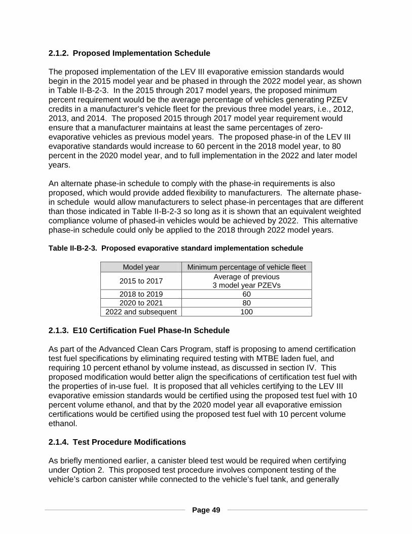
Page 49
2.1.2. Proposed Implementation Schedule The proposed implementation of the LEV III evaporative emission standards would begin in the 2015 model year and be phased in through the 2022 model year, as shown in Table II-B-2-3. In the 2015 through 2017 model years, the proposed minimum percent requirement would be the average percentage of vehicles generating PZEV credits in a manufacturer’s vehicle fleet for the previous three model years, i.e., 2012, 2013, and 2014. The proposed 2015 through 2017 model year requirement would ensure that a manufacturer maintains at least the same percentages of zero-evaporative vehicles as previous model years. The proposed phase-in of the LEV III evaporative standards would increase to 60 percent in the 2018 model year, to 80 percent in the 2020 model year, and to full implementation in the 2022 and later model years.
An alternate phase-in schedule to comply with the phase-in requirements is also proposed, which would provide added flexibility to manufacturers. The alternate phase-in schedule would allow manufacturers to select phase-in percentages that are different than those indicated in Table II-B-2-3 so long as it is shown that an equivalent weighted compliance volume of phased-in vehicles would be achieved by 2022. This alternative phase-in schedule could only be applied to the 2018 through 2022 model years. Table II-B-2-3. Proposed evaporative standard implementation schedule
Model year Minimum percentage of vehicle fleet
2015 to 2017 Average of previous 3 model year PZEVs
2018 to 2019 60 2020 to 2021 80
2022 and subsequent 100 2.1.3. E10 Certification Fuel Phase-In Schedule As part of the Advanced Clean Cars Program, staff is proposing to amend certification test fuel specifications by eliminating required testing with MTBE laden fuel, and requiring 10 percent ethanol by volume instead, as discussed in section IV. This proposed modification would better align the specifications of certification test fuel with the properties of in-use fuel. It is proposed that all vehicles certifying to the LEV III evaporative emission standards would be certified using the proposed test fuel with 10 percent volume ethanol, and that by the 2020 model year all evaporative emission certifications would be certified using the proposed test fuel with 10 percent volume ethanol. 2.1.4. Test Procedure Modifications As briefly mentioned earlier, a canister bleed test would be required when certifying under Option 2. This proposed test procedure involves component testing of the vehicle’s carbon canister while connected to the vehicle’s fuel tank, and generally

Page 50
mimics the two-day test procedure. In this procedure, the canister would be stabilized to a 4,000-mile test condition and preconditioned through loading and purging. The canister would then be connected to the fuel tank vent port, and both the canister system and the fuel tank placed in a testing enclosure where the ambient temperature is cycled between 65°F and 105°F, for a period of two 24-hour cycles. To determine compliance with the proposed canister bleed test, the amount of hydrocarbons emitted over each 24-hour period would have to be equal to or less than the proposed emission standard. The proposed canister bleed test requires substantially less time and is less labor-intensive than the rig test manufacturers currently perform for the zero-evaporative emission standards, although the canister bleed test is not as comprehensive as the rig test, which tests every evaporative emission control and fuel system component. However, staff believes the proposed canister bleed test and standards coupled with the proposed Option 2 lower whole vehicle standards would be equally effective in ensuring equivalent emission control as the current zero-evaporative emission standards. 2.1.5. Pooling Evaporative Emissions from California and Section 177 States Beginning in 2015, staff is proposing to provide an option to allow compliance with the fleet average Highest Diurnal plus Hot Soak requirement, set forth in section II.B.2.1.1.b., be demonstrated using the pooled fleet average of the Highest Diurnal plus Hot Soak emission values of new vehicles produced and delivered for sale in California and all states, including the District of Columbia if applicable, that adopt California’s evaporative emission requirements for light-, medium-, and heavy-duty vehicles. Staff is also proposing to allow pooling to comply with the phase-in requirements discussed in section II.B.2.1.2. Manufacturers that choose this option would be required to report the number of vehicles produced and delivered for sale and the emission standards, and family emission limits, if applicable, to which they are certified for each state, and the District of Columbia if applicable, that adopts California emission requirements. Including this provision provides additional compliance flexibility to vehicle manufacturers, particularly with respect to meeting a separate fleet average requirement in those states with limited new vehicle sales. While this represents a departure from past practice, staff believes that the emission impact of this provision within California and states that adopt California requirements will be minor due to the very low level of fleet emissions required by this program. 2.2. Proposed Onboard Refueling Vapor Recovery (ORVR) Amendments The ORVR regulations were previously updated in 2009 for changes related to plug-in hybrid vehicles. The changes proposed in LEV III are to bring the applicability of ORVR standards into alignment with the current federal regulations and expected Tier 3 amendments to 40 CFR §86-1811-04(e)(3). California’s current ORVR standards (13 CCR §1978) only apply to vehicles up to 8,500 pounds GVWR. The proposed change would increase the applicability of the ORVR requirements to complete vehicles up through 14,000 pounds GVWR inclusive. The proposed regulatory language for section 1978, title 13, CCR is provided in Appendix A. The “California Refueling Emission

Page 51
Standards and Test Procedures for 2001 and Subsequent Model Motor Vehicles” is incorporated by reference into section 1978, title 13, CCR and proposed revisions to the incorporated test procedures are provided in Appendix G. Under the current federal ORVR regulations, complete vehicles up through 10,000 pounds GVWR are required to meet the ORVR standards. However, OEMs have indicated that complete vehicles up through 14,000 pounds GVWR contain ORVR equipment in an effort to minimize evaporative system variants among the MDV class. Thus, to come into alignment with current practice and prevent future backsliding, staff is proposing that, beginning with model year 2015, complete vehicles up through 14,000 pounds GVWR comply with the ORVR standards. The proposed LEV III standards are unchanged from the LEV II standards of 0.20 grams hydrocarbons per gallon of fuel dispensed for gasoline-fueled, diesel-fueled, and hybrid electric vehicles (hydrocarbons mean organic material hydrocarbon equivalent for alcohol-fueled vehicles), and 0.15 grams hydrocarbons per gallon of fuel dispensed for liquefied petroleum gas-fueled vehicles. In addition to increasing the GVWR applicability, staff is proposing an option to allow OEMs to use California certification fuel (gasoline with 10 percent ethanol) during the certification testing in lieu of federal certification fuel, with the provision that California test temperatures are also used (Appendix G). This change is being proposed to allow streamlining between the ORVR and evaporative emission testing when California certification fuel is used for evaporative emission testing. The proposed increase in the refueling temperature from 67°F ± 1.5°F to 79°F ± 1.5°F if California certification fuel is used would ensure comparability with the federal test procedures and test fuels, which have a higher vapor pressure but lower test fuel temperature. The vehicle soak temperature would remain unchanged in order to ensure equivalent stringency regardless of the certification fuel used. The proposed changes to the ORVR regulations and test procedures are not expected to result in any emission reduction or OEM cost due to current federal requirements for vehicles 8,501 through 10,000 pounds GVWR, OEM practice for vehicles 10,000 through 14,000 pounds GVWR, and use of on-site vapor recovery at refueling stations located in ozone non-attainment areas. Thus, these proposed changes serve to harmonize California and federal regulatory requirements and ensure the best available refueling vapor recovery systems on all complete vehicles equal to or less than 14,000 pounds GVWR. 2.3. Proposed Amendments to the Specifications for Fill Pipes and Openings of Motor Vehicle Fuel Tanks The specifications for fill pipes and openings of motor vehicle fuel tanks (13 CCR §2235) were last amended in 1990 and were based upon Society of Automotive Engineers (SAE) specifications that have since been withdrawn and superseded by the International Organization for Standardization (ISO) standard, “Road vehicles – Filler pipes and openings of motor vehicle fuel tanks – Vapour recovery system” (ISO 13331-

Page 52
1995(E)). This ISO standard is based upon the original SAE standards, but addresses several errors and clarifies aspects of the design criteria. In order to bring the “Specifications for Fill Pipes and Openings of Motor Vehicle Fuel Tanks” up to date with the most current industry standards, staff is proposing to revise the current specifications so that they would be applicable only through model year 2014 (Appendix H). Beginning with model year 2015, the specifications based on the SAE standards ("Specifications for Fill Pipes and Openings of 1977 through 2014 Model Motor Vehicle Fuel Tanks") would be sunsetted and replaced by new specifications that incorporate the ISO standards by reference ("Specifications for Fill Pipes and Openings of 2015 and Subsequent Model Motor Vehicle Fuel Tanks"). The proposed specification language for 2015 and subsequent model year vehicles is available in Appendix I. Because the fill pipe specifications in the ISO-13331-1995 standard are substantially similar to and primarily clarifications of the SAE specifications referenced in the 1990 revision of 13 CCR Section §2235, no OEM changes for compliance are anticipated. All test procedures would continue to be required and would be unchanged from the 1990 amendments. 3. TECHNOLOGICAL FEASIBILITY OF PROPOSED STANDARDS 3.1. Current Evaporative Emission Technology Today’s most advanced evaporative emission control technologies are in vehicles meeting the optional zero-evaporative emission standards. The current state-of-the-art in evaporative technology is described in the ensuing paragraphs. Evaporative emission control technology can basically be grouped into three categories: carbon canister system, fuel storage / delivery system, and air intake system. 3.1.1. Carbon Canister System A carbon canister system is employed to adsorb hydrocarbon vapors generated in the fuel tank during a refueling event, during vehicle operation, and while the vehicle is parked. These vapors are adsorbed by activated carbon granules contained in the canister. Canister system emissions generally fall into two categories: breakthrough and bleed. In a typical evaporative test sequence, breakthrough is the point when 2.0 grams of hydrocarbon has been emitted from the canister. The canister system emissions that occur before the onset of breakthrough are bleed emissions. Target canister system emission levels for zero-evaporative vehicles are in the 0.003-0.010 gram/test range. These bleed emissions occurring at this level are not due to lack of adsorptive capacity in the canister, but are due to diffusion (i.e., transfer of adsorbed fuel molecules through the canister to the port which is open to the atmosphere) (Williams et al. 2001). The majority of zero-evaporative vehicles incorporate a hydrocarbon scrubber in order to achieve very low level bleed emissions. Most often, the scrubber is an auxiliary activated carbon honeycomb attached to the canister’s atmosphere port. Simulated real

Page 53
time two-day diurnal testing, at 150 bed volumes of purge, yielded emissions of 0.196 grams with a standard canister, which were reduced to 0.015 grams with the addition of a hydrocarbon scrubber (Williams et al. 2001). 3.1.2. Fuel Storage and Delivery System
Fuel permeation through the fuel tank, fuel lines, and vapor lines, combined with leakage from the associated connections for these components, contribute to evaporative emissions. In the fuel systems of current zero-evaporative vehicles, both system configuration and materials selection are optimized to achieve minimal evaporative emissions. A system that has a minimal number of connections and components exposed to the atmosphere will have fewer opportunities for leakage. One current design practice involves integrating components such as venting valves, the fuel filter, and the fuel pump inside the fuel tank. Some fuel tanks use a common entry port for these internal components. For sealing off exposed components and critical joints, such as the fuel tank inlet, some designs include an external barrier film application. Hydrocarbon permeation is reduced in current fuel system designs by minimizing the permeable materials’ fuel exposure area and incorporating low/no permeation materials. Steel and plastic are used for the rigid components of the fuel system. Gasoline and alcohol do not permeate steel, while with plastic, permeation does occur, but this is drastically reduced by adding barrier layer(s) composed of low permeation materials. Rigid component barrier layer materials such as ethylene vinyl alcohol (EVOH) and fluoropolymers have shown good performance in limiting permeation with ethanol-containing fuels (Nulman et al. 2001). For seal, gasket, and hose applications, fluoroelastomers have been shown to limit permeation from ethanol containing fuels while retaining the mechanical properties required for a robust seal (Thomas et al. 2009). Staff expects that the proposed test fuel containing 10 percent ethanol would result in a small increase in evaporative emissions during certification testing in comparison to certification tests conducted using the current MTBE-based fuel with no ethanol. The expected increase in certification emissions would be due to increased permeation, which can increase fuel system hydrocarbon emissions by as much as 0.028 grams on a zero-evaporative passenger car (Haskew et al. 2006). However, most vehicles currently contain low-permeation materials because manufacturers must design for the commercial fuel in California, which contains up to 10 percent ethanol. Therefore, staff does not expect manufacturers to make significant changes to the fuel system to accommodate the proposed test fuel, nor does staff expect any impact on fleet evaporative emissions due to the change.

Page 54
3.1.3. Air Intake System Evaporative Controls
The vehicle’s air intake system (AIS) is another channel from which evaporative emissions can escape. These emissions result when fuel injector leakage, vapors from uncombusted fuel in the intake manifold, and crankcase blow-by gases escape out of the vehicle’s AIS. AIS emissions occur when the engine is turned off and the engine compartment is exposed to residual engine heat in addition to heat from diurnal temperature variations. The majority of current zero-evaporative vehicles are equipped with some form of AIS emission control element. Non-zero-evaporative vehicles are typically certified without an AIS element. An AIS control element is typically placed in either the vehicle’s airbox or in the air tube between the throttle body and the airbox. The AIS element adsorbs hydrocarbon vapors that pass by or through it by the means of an activated carbon or synthetic Zeolite material. Similar to the carbon canister’s functionality, when the engine is operated, the hydrocarbons adsorbed on the AIS element are drawn into the engine for combustion. These devices are designed to be permanently installed and maintain their function for the vehicle’s full useful life. 3.2. Potential Technologies for Compliance with Proposed Standards Staff expects that the fuel system and evaporative control technology package required for a vehicle to meet the proposed standards would be equivalent to what is in today’s zero-evaporative vehicle. However, hybrid vehicles could require some additional technology to meet the proposed bleed emission test standard, because they have less available purge to regenerate the carbon canister. Since the internal combustion engine in a hybrid may be turned off for long periods during vehicle operation, there are fewer opportunities to purge the canister. Purge volume is normally expressed in terms of canister bed volumes displaced during the two-day test procedure. Currently, a non-hybrid zero-evaporative vehicle yields 150-250 bed volumes while, in contrast, a hybrid with an integrated evaporative system produces 70-100 bed volumes. A trend of decreasing available purge is expected for future hybrid vehicles, due to increased time in engine-off mode. A partially pressurized fuel tank is expected to be one of the most feasible technologies to compensate for hybrid vehicles’ lower available purge. Since the fuel tank would be sealed up to a particular threshold pressure, this technology would facilitate reduced canister loading. Heated purge may be another option for addressing low-purge by increasing the efficiency of a given purge volume.

Page 55
4. COST ANALYSIS 4.1. Cost methodology Staff has estimated the cost to auto manufacturers to implement the proposed changes to the evaporative emission program. Cost information was obtained by consulting with fuel system suppliers, vehicle manufacturers, and USEPA. A typical vehicle meeting the current LEV II evaporative standards was used as the baseline for determining incremental costs. 4.2. Cost Analysis Table II-B-4-1 shows an estimate of the added cost per vehicle for various parts of the fuel and evaporative control system to meet the proposed standards. The majority of the costs are expected to be due to the expansion of existing zero-evaporative technology. Some manufacturers have already integrated zero-evaporative components to a large extent on the rest of their fleet, which should reduce their compliance costs. The cost values noted below have been weighted based upon the fact that it takes a combination of the modifications listed below, not necessarily all of them, to achieve a zero-evaporative system. Four dollars of indirect costs were added to account for overhead as well as fixed (one time) costs that would be incurred in a small proportion of cases requiring a new component design for an in-house manufactured part, such as a fuel tank. Staff does not expect there to be a substantial difference in incremental cost among the various vehicle weight categories. The heavier vehicles would require more materials, but this should balance out cost-wise since the additional space allows for a more simple design and layout of fuel system components.
Table II-B-4-1. Evaporative Technologies’ Incremental cost
Component Changes Added cost per vehicle
Fuel tank
Minimize ports (locate vents and valves inside tank, entry through a common port), low permeation material, vapor
block valve for hybrids
$2.90
Canister Addition of hydrocarbon scrubber $10.00 AIS System Addition of control element $2.00
Fuel lines and system connections
Fewer components, low permeation material $2.10
Total direct manufacturing costs $17
Total + $4.00 indirect costs $21

Page 56
5. OUTSTANDING ISSUES During the development of the evaporative emission proposal, staff deliberated with affected vehicle manufacturers on various issues related to the rulemaking. In addition, staff held several rulemaking workshops for the general public to solicit feedback on the proposal. Although most of the rulemaking issues have been resolved, there is one remaining issue that is still under consideration. This issue pertains to vehicle evaporative emissions as measured in the field. A recent USEPA test program showed that for many vehicles, in-use evaporative emissions are much higher than those observed during certification, indicating the need to strengthen current certification and in-use compliance programs. Although test data on current zero-evaporative emission vehicles (i.e., PZEVs) are limited, it is expected that the materials and connections used to meet the proposed LEV III evaporative emission requirements will reduce emissions over the lifetime of the vehicle, in part by reducing in-use deterioration. Current on-board diagnostic (OBD) systems also monitor for evaporative system leaks, although not all leaks may be detected and the onus is on the vehicle owner to have the leak repaired. Thus, if even a small percentage of vehicles develop leaks in-use, significant gains from LEV III could be lost. As such, ARB staff is working with EPA to develop a leak emission standard and test procedure. A requirement that vehicles be subject to a “leak test” requirement both at certification and in-use could be incorporated into LEV III when the currently proposed rule is finalized or, more likely, through a separate rulemaking in the future. Because fuel system leaks develop as vehicles age and new systems are unlikely to fail the leak test as proposed, it is anticipated that manufacturers would be given the option to provide an attestation of compliance at certification, with compliance testing conducted primarily during the in-use verification program. Although ARB, USEPA, and industry are still working on the details of the leak test, a general outline of the procedure is provided in Figure II-B-5-1. The leak test would utilize a test apparatus that would attach to the vehicle fuel system, either through a dedicated test port or through a fuel system opening such as the filler pipe. The fuel system would then be sealed and slightly pressurized (less than 0.5 pounds per square inch) with an inert gas. The test apparatus would be calibrated such that at a given temperature and system pressure, the flow of gas through the apparatus corresponds to the leak size. For example, a larger leak in the fuel system would be correlated with a higher flow rate through the apparatus due to the need for more inert gas to maintain a given pressure as gas is lost through the leak(s). It is expected that the certification and in-use standards for maximum permissible orifice size will be set between 0.01 and 0.02 inches. Staff anticipates that manufacturers would be able to conduct this test either in sequence with the current 2-day or 3-day diurnal test procedure or as a stand-alone test procedure utilizing the same preconditioning procedures as the diurnal tests. This requirement would complement the OBD evaporative system leak monitoring requirement, not replace it.

Page 57
Calibrate and/or verify testing apparatus
Precondition vehicle similar to diurnal test (fuel to 40%, soak 6 hours)
Seal fuel system so as to pressure test entire system (purge valve, cap, etc.)
Attach tester to vehicle’s fuel system
Pressurize fuel system with inert gas (max 0.5 psi)
Allow flow and pressure to stabilize
Determine effective leak size from output data
Calculated effective leak size must be less than 0.01 - 0.02 inches
Figure II-B-5-1. Flow chart depicting the outlined procedure for the proposed leak test.
While detailed regulatory text for the leak test requirement is not currently proposed as part of the LEV III evaporative emissions program, staff proposes that the LEV III/GHG regulatory proposal, as part of the Advanced Clean Cars rulemaking package, be finalized with the final federal leak test and standard as described, provided it is substantially similar to that depicted in Figure II-B-5-1. ARB staff anticipates that USEPA will incorporate the leak test and associated standards when the Tier 3 rulemaking is finalized in 2012, at which time ARB staff will evaluate whether this test requirement should be included into LEV III for certification and in-use verification

Page 58
purposes. Assuming staff determines that the leak test and standard are appropriate for inclusion into LEV III, the finalized federal regulatory language, as modified by California, would be subject to additional public comment – ideally occurring before ARB has finalized the current rule – in order to promote harmonization within the national program. 6. REGULATORY ALTERNATIVES TO EVAPORATIVE EMISSION PROPOSAL As part of the regulatory development process, the following alternatives to this proposal were considered. 6.1. Do Not Amend the Evaporative Emission Standards To continue to reduce smog-forming VOC emissions, staff believes it is necessary to increase the stringency of the current evaporative standards. Based on staff’s analyses, the proposed regulation is feasible and cost-effective since for the most part, it would require only expansion of existing zero-evaporative technology. 6.2. Adopt More Stringent Evaporative Emission Standards 6.2.1. Zero-fuel test requirement Extending the zero fuel, or rig test, to the entire fleet was seen as a way to reduce evaporative emissions. However, manufacturers contend that this test is excessively burdensome due to the complexity and cost of setting up fuel system rigs, and the new test facilities that would be required. Option 2, with the lower whole vehicle standard and the canister bleed test, has been proposed to give manufacturers an alternative to the rig test. Staff considers Option 2 to provide equivalent emission control as compared to the higher whole vehicle standard and rig test which make up the current zero-evaporative requirement. This rig test will be an option for manufacturers, as it is contained in the proposed Option 1. 6.2.2. Lower whole vehicle emission standard Staff believes that the fuel systems on vehicles certified to the zero-evaporative emission standard represent the best of currently available evaporative control technology. A large proportion of the evaporative emissions on zero-evaporative certified vehicles come from non-fuel sources. Although there are current zero-evaporative vehicles with two-day and three-day diurnal plus hot soak certification levels below 0.150 grams, these vehicles have very low background (non-fuel) emissions, which staff believes would be very difficult to achieve on an average fleet-wide basis. Based upon a review of average zero-evaporative vehicle certification values, staff believes that the proposed emission standards are appropriate to expand the use of zero-evaporative technology to the rest of the fleet, and that a lower whole vehicle emission standard would not allow sufficient margin for non-fuel evaporative emissions.

Page 59
C. VEHICLE LABELING REQUIREMENTS 1. BACKGROUND Since 1995, California’s Smog Index Label helped consumers assess the relative smog emissions from new cars. In 2005 Assembly Bill 1229 was signed into law (Nation, Chap. 75, Stats. 2005, codified at Health and Safety Code §43200.1). These amendments to California’s vehicle labeling regulations created a more user-friendly scoring system for determining the Smog Score and added a Global Warming Score. Both scores are based on a scale of 1 -10 with 10 being the cleanest and 5 representing an average new car. The California Environmental Performance Label (Figure II-D-1-1) is required on all new vehicles sold in California that were manufactured after January 1, 2009. Figure II-D-1-1. California Environmental Performance Label
Per the Energy Independence and Security Act of 2007, the United States Department of Transportation, United States Department of Energy and USEPA were directed to revise the Federal Fuel Economy Label to reflect an automobile’s fuel economy and greenhouse gas and other emissions over the useful life of the automobile. It also required the revised label to include a rating system that would make it easy for consumers to compare the fuel economy and greenhouse gas and other emissions at the point of purchase. Starting in the Spring of 2010, ARB staff began working with USEPA and NHTSA on revisions to the Fuel Economy Label. The goal of working with USEPA and NHTSA was to provide input on the information needed on the Federal label to allow California to use this Label in lieu of the California Environmental Performance label.

Page 60
Important California requirements addressed by the federal label included: • Adding the following statement to the label: “Vehicle emissions are a significant
cause of climate change and smog” • Having a clear statement about upstream emissions and having a clear place to
find this information on a regional basis. • Including all cars in the rating system rather than segregating by size or class. Because of this successful collaboration California is able to harmonize with the federal labeling requirements. In June 2011, USEPA and NHTSA published 40 CFR Parts 85, 86, and 600 providing requirements for the new Fuel Economy and Environment Label meeting these requirements. This new Federal Label (Figure II-D-1-2) is required on all new cars starting with Model Year 2013 and can be affixed earlier on a voluntary basis. The new Federal Fuel Economy and Environment Label is a redesign that now includes a Greenhouse Gas and Fuel Economy Rating from 1 to 10 with 10 being best and a Smog Rating, also from 1 to 10 with 10 being cleanest. The content and graphical design are sufficiently similar to and were inspired by the Global Warming and Smog Scores on California’s Environmental Performance Label. Figure II-D-1-2. Federal Fuel Economy and Environment Label, June 6, 2011
Page 61
2. SUMMARY OF PROPOSED REGULATION Staff is proposing to add language to the “California Smog Index Label Specifications for 2009 and Subsequent Model Year Passenger Cars, Light-Duty Trucks, and Medium-Duty Passenger Vehicles,” incorporated by reference at Title 13, California Code of Regulations, Section 1965), that would deem manufacturer compliance with the Federal Fuel Economy and Environment Label published in 40 CFR Parts 85, 86, and 600 as promulgated on July 6, 2011 as compliant with the California Environmental Performance Label requirements. Providing consumers with only one label that includes substantial environmental information meeting California’s statutory requirements will avoid confusion as well as information overload. Staff is also proposing to add clarifying language about Neighborhood Electric Vehicles (NEVs). NEVs are not permitted to affix the Federal Fuel Economy and Environment Label because only those vehicles that qualify for Corporate Average Fuel Economy (CAFE) credits are permitted to have these labels. Since NEVs cannot receive these credits, they cannot affix this label. Therefore, for consistency, staff proposes to no longer require the Environmental Performance Label on these types of vehicles. 3. COST ANALYSIS By allowing OEMs to use the new Federal Fuel Economy and Environment to meet the California’s vehicle labeling requirements, OEMs will save money by not having to also print and affix the California Environmental Performance Label. According to the May 4, 2007 Initial Statement of Reasons for the Environmental Performance Label, the initial annualized cost for compliance for the industry as a whole with these requirements was estimated to be $3,500 and the annual ongoing cost for a typical manufacturer was estimated to be $4,667, making an OEM’s total annual cost for printing the California Environmental Performance Label and affixing it to all of their cars to be $8,167. Although the initial annualized costs will not change, the ongoing annual cost will go to zero. D. MINOR AMENDMENTS TO THE ON-BOARD DIAGNOSTICS REGULATIONS 1. BACKGROUND Second generation on-board diagnostics (OBD II) systems are comprised mainly of software designed into the vehicle’s on-board computer to detect emission control system malfunctions as they occur by monitoring virtually every component and system that can cause an increase in emissions. When an emission-related malfunction is detected, the OBD II system alerts the vehicle owner by illuminating the malfunction indicator light (MIL) on the instrument panel. By alerting the owner of malfunctions as they occur, repairs can be sought promptly, which results in fewer emissions from the vehicle. Additionally, the OBD II system stores important information including identification of the faulty component or system and the nature of the fault, which would

Page 62
allow for quick diagnosis and proper repair of the problem by technicians. This helps owners achieve less expensive repairs and promotes repairs done correctly the first time. With OBD II systems having been required on all 1996 and newer vehicles produced for sale in California and most vehicles sold nationwide, more than 110 million vehicles are currently equipped with them. Input from manufacturers, service technicians, inspection and maintenance (I/M) programs, and in-use evaluation programs indicate that OBD II systems are very effective in finding emission problems and facilitating repairs. Accordingly, US EPA issued a final rule indicating its confidence in the performance of OBD II systems by requiring states with I/M programs to perform OBD II checks for these newer cars and allowing them to be used in lieu of current tailpipe tests. The California I/M program (Smog Check) has adopted these provisions. The California Air Resources Board (ARB) originally adopted the light- and medium-duty vehicle OBD II regulation in 1989 for the 1994 and newer model years. As directed by the Board, the regulation has been reviewed and updated at regular updates since then, with the last major update to the regulation occurring in 2006 as well as updates to the medium-duty diesel requirements occurring in 2009. Staff was not scheduled to go to the Board this year to update the OBD II regulation; however, manufacturers recently approached ARB staff and requested regulation changes that they indicated were needed immediately in order to ensure compliance when they certify their 2013 model year vehicles. Manufacturers and ARB staff held discussions with interested manufacturers, including a face-to-face meeting on July 27, 2011, to discuss their proposal. In response to the manufacturers’ requests, staff is proposing changes to the OBD II regulation, California Code of Regulations (Cal. Code Regs.), title 13, section 1968.2, and its associated enforcement regulation, section 1968.5. 2. SUMMARY OF PROPOSED AMENDMENTS
Section 1968.2(c): Definitions The OBD II regulation currently defines “calculated load value” for diesels as “determined by the ratio of current output torque to maximum output torque at current engine speed as defined by suspect parameter number (SPN) 92 of SAE J1939.” Manufacturers have indicated that the definition in Society of Automotive Engineers (SAE) J1939 only applies to heavy-duty diesel engines, so they need a comparable definition that would apply to light- duty and medium-duty diesel vehicles. Thus, ARB staff is proposing to modify the language to allow manufacturers to use the definition of “calculated load value” that was recently amended in SAE J1979 for diesel vehicles. The OBD II regulation currently allows manufacturers to erase a confirmed fault code if the identified malfunction has not been again detected in at least 40 engine warm-up cycles and the MIL is presently not illuminated for that malfunction. The regulation

Page 63
currently defines “warm-up cycle” as “sufficient vehicle operation such that the coolant temperature has risen by at least 40 degrees Fahrenheit from engine starting and reaches a minimum temperature of at least 160 degrees Fahrenheit (140 degrees Fahrenheit for applications with diesel engines).” Manufacturers have expressed concern that certain vehicles such as hybrid vehicles or vehicles with highly efficient engines may not be able to meet these temperature criteria under normal driving and ambient conditions. Thus, manufacturers have requested language that allows manufacturers to use an alternate minimum temperature criterion. Staff understands that some allowances should be made for such vehicles that are unable to warm-up the engine coolant temperature to the defined temperatures even if it has been sufficiently driven. Thus, staff is proposing to allow manufacturers the option to define a “warm-up cycle” as a driving cycle in which the criteria to erase a permanent fault code for continuous monitors are met (sections 1968.2(d)(2.5.2)(B)(iii)a., b. and c.). This would ensure that the vehicle has been operated for a sufficient period of time to reasonably detect a recurrence of the malfunction but does not delay erasure of confirmed fault codes. Staff is proposing changes to the permanent fault code erasure requirements and the in-use monitor performance requirements that would apply to hybrid vehicles, details of which are described below. Given the context of the proposed changes, new definitions would be needed to complement the proposed requirements. Thus, staff is also proposing four new definitions for “hybrid vehicle,” “plug-in hybrid electric vehicle,” “fueled engine operation,” and “propulsion system active” to supplement the proposed changes. More details about the proposed definitions can be found below. Section 1968.2(d)(2.5): Erasing a Permanent Fault Code The OBD II regulation requires the OBD II system to store a “permanent” fault code for an emission-related fault in non-volatile memory that can only be erased if the monitor responsible for setting that fault code has run and passed enough times to confirm that the fault is no longer present. Currently, the regulatory language (section 1968.2(d)(2.5.1)) states that the permanent fault code can be erased “only if the OBD II system itself determines that the malfunction that caused the permanent fault code to be stored is no longer present and is not commanding the MIL on, pursuant to the requirements of section (d)(2.3) (which for purposes of this section shall apply to all monitors).” Manufacturers have expressed confusion about the exact timing of erasing the permanent fault code. Thus, staff is proposing to clarify the requirement by adding language indicating that erasure of the permanent fault code shall occur in conjunction with extinguishing the MIL or no later than the start of the first driving cycle that begins with the MIL commanded off. Additionally, staff is proposing changes to address issues concerning permanent fault code erasure on hybrid vehicles for monitors that are designed to run continuously, including monitors that must wait until similar conditions are satisfied (e.g., gasoline misfire and fuel system monitors). Currently, the regulation requires that the permanent fault code for these monitors be erased only after the vehicle has been operated such

Page 64
that, among other conditions, criteria similar to those for a general denominator (section 1968.2(d)(4.3.2)(B)) have been satisfied on a single driving cycle (with the exception that the general denominator conditions require ambient temperature above 20 degrees Fahrenheit or below 8000 feet in elevation). This ensures that the vehicle has been operated for a sufficient period of time to reasonably detect a recurrence of the malfunction but does not unnecessarily delay erasure of the permanent fault code. Among these conditions is the criterion that the “cumulative time since engine start” be greater than or equal to 600 seconds. Manufacturers have indicated that changes are needed to account for the fact that hybrid vehicles, especially plug-in hybrids, may encounter a significant number of driving cycles where the engine starts very late (if at all) in a typical drive cycle and the cumulative amount of engine runtime is limited. Thus, for hybrid vehicles, staff is proposing to clarify that manufacturers should use 600 cumulative seconds of “propulsion system active” time in lieu of the 600 cumulative seconds after engine start, with “propulsion system active” defined as when the vehicle is operated, regardless of whether it is powered by the battery or the engine or both. Staff believes this new definition would ensure equivalent vehicle operation time between conventional vehicles and hybrid vehicles. Further, the new language is consistent with how manufacturers have been implementing such counters to date on hybrid vehicles but the clarifications will provide more guidance especially to those that have not yet certified hybrid vehicles. Sections 1968.2(d)(3.2), (d)(4.3.2), and (d)(5.5) and Section 1968.5: In-Use Monitor Performance Specifications The OBD II regulation requires manufacturers to track monitor performance by counting the number of monitoring events and the number of driving events. The number of monitoring events is defined as the numerator and the number of driving events is defined as the denominator. The ratio of these two numbers is referred to as the monitoring frequency and provides an indication of how often the monitor is operating relative to vehicle operation. The regulation also requires all vehicles to keep track of a “general denominator”, which is a measure of how often the vehicle is operated. The regulation requires manufacturer to increment this denominator only if certain criteria are satisfied on a single driving cycle. This method allows very short trips or trips during extreme conditions such as very cold temperatures or very high altitude to be filtered out and excluded from the count. This is appropriate because these are also conditions where most OBD II monitors are neither expected nor required to operate. The regulation currently requires all vehicles to increment the general denominator if, among other conditions, the “cumulative time since engine start” is greater than or equal to 600 seconds. For the same reasons noted above, hybrid vehicles, especially plug-in hybrids, need an alternate definition to recognize trips where the engine does not start or starts much later in the trip. Manufacturers are concerned that with the current regulatory language, the general denominator will increment more often than it should compared to how often the monitors will have had a chance to run in-use (i.e., how long the engine will actually be turned on) and are concerned that the resulting ratios will not be able to meet the minimum required ratios. They further argued that this may force

Page 65
them to increase engine operation just to run the monitors to meet the required ratios, which would reduce vehicle efficiency and basically reduce the advantages of the plug-in capability. Staff agrees that some changes are needed to account for these issues. Thus, similar to the changes proposed above for the permanent fault code erasure protocol, for hybrid vehicles, staff is proposing to clarify that manufacturers must use 600 cumulative seconds of “propulsion system active” time in lieu of the 600 cumulative seconds after engine start when incrementing the general denominator. Additionally, staff is also proposing to require 10 seconds of “fueled engine operation” to be met in order to increment the general denominator to discern between trips with and without engine operation. This condition would ensure that only trips where the engine has at least turned on once during the driving cycle are counted when looking at how often engine-related emission control component monitors are running. These proposed changes would apply to 2014 and subsequent model year hybrid vehicles. Additionally, manufacturers indicated changes are needed to the denominator incrementing criteria for evaporative system monitors. Unlike tailpipe emissions where the engine has to operate in order for emissions to occur, evaporative emissions such as gasoline vapor escaping from the gasoline tank to the atmosphere can occur from a vehicle while it is parked or being operated off of battery power. Accordingly, the evaporative system monitors need to work, regardless of how often the engine is actually started or used on the vehicle. The regulation currently requires the evaporative system monitor denominator to be incremented only on trips that meet a ‘cold start’ definition (i.e., if the engine coolant temperature (ECT) and the ambient temperature are considered cold and the ECT at engine start is less than or equal to 12 degrees Fahrenheit higher than ambient temperature at start). The criteria were set to ensure that the vehicle has had a long enough soak period such that the evaporative system (fuel tank, canister, etc.) will have cooled down and stabilized by the beginning of the driving cycle and it would be technically feasible to run a robust evaporative system monitor. While this current ‘cold start’ definition works adequately for conventional vehicles and traditional hybrids, manufacturers have argued that plug-in hybrid electric vehicles will have some driving cycles that are all-electric and that the definition does not address such conditions. Specifically, the existing definition could result in multiple increments of the evaporative system monitor denominator after short all-electric drive trips even though the evaporative system is no longer at a stabilized condition because ECT will still be within the cold start-defined window relative to ambient temperature. Staff agrees that changes are needed to avoid these issues and is proposing alternative criteria for plug-in electric hybrid vehicles that would better ensure a long soak period similar to that on conventional vehicles and traditional hybrids. Specifically, for 2015 and subsequent model year plug-in hybrid electric vehicles, staff is proposing that the denominator be incremented when the soak period immediately preceding the driving cycle is greater than or equal to 6 hours in lieu of requiring the ECT at engine start to be less than or equal to 12 degrees Fahrenheit higher than ambient temperature at start. For example, a conventional car would first look at ECT and ambient temperature at engine start, make sure they agree with each other to confirm it is a cold start of the

Page 66
vehicle, make sure ambient temperature is within acceptable ranges, and then look for the drive cycle to meet the rest of the criteria to count as an evaporative system denominator trip. Plug-in hybrids, however, would instead first look at the amount of time the vehicle has been off/not operated when the vehicle is first started, make sure that it has been at least 6 hours since the previous vehicle trip to confirm it is a cold start of the vehicle, and then make sure the ambient temperature is within range and that the drive cycle meets the rest of the criteria to count as an evaporative system denominator trip. For additional flexibility to manufacturers, plug-in hybrid electric vehicles built prior to the 2015 model year would have the option of using these new criteria or the existing criteria to increment the evaporative system monitor denominator. Manufacturers have also argued that a smaller minimum required ratio is needed to account for the limited engine operation time for plug-in hybrid vehicles and to allow them to maximize electric operation/minimize CO2 emissions. While staff believes some relief is needed with respect to the ratio, staff believes a smaller ratio is only needed for the interim years considering the proposed revisions to the denominator criteria above would already provide substantial relief in meeting the in-use performance ratio requirements relative to conventional vehicles. Thus, staff is proposing that for monitors of components or systems that require engine operation on plug-in hybrid electric vehicles, manufacturers would be required to meet a minimum ratio of 0.100 in lieu of the current higher ratios (e.g., 0.336 for most monitors) through the 2016 model year. This would allow manufacturers to run monitors less frequently on plug-in hybrids and still be considered compliant. Starting with the 2017 model year, the interim relief would end and these monitors would be required to meet the higher minimum ratios currently required in the regulation. However, staff will also plan to revisit this requirement once plug-in hybrid electric vehicles are in-use and data are available to better strike a balance between monitoring frequency (to detect emission faults in a timely manner) and reduced engine operation (and the resultant CO2 emissions). Staff is also accordingly proposing changes in the OBD II enforcement regulation (Cal. Code Regs., title 13 section 1968.5) to account for the newly proposed ratio when determining OBD II non-compliances for plug-in hybrid electric vehicles. Lastly, staff is proposing changes to the ignition cycle counter requirements for hybrid vehicles and plug-in hybrid electric vehicles. Currently, manufacturers are required to track and report an ignition cycle counter, which is required to be incremented every time the vehicle is started (i.e., “engine start” is met). This is basically a counter of the number of driving cycles experienced by the vehicle. First, staff is proposing to modify the incrementing criteria for hybrid vehicles – specifically, staff is proposing to clarify that manufacturers increment the ignition cycle counter when the “propulsion system active” definition is met (e.g., each time the vehicle is operated, without respect to whether the engine is started or used). This is consistent with how hybrid manufacturers have been tracking this counter to date. Second, staff is proposing that 2014 and subsequent model year plug-in hybrid electric vehicles track and report an additional, separate ignition cycle counter that would be incremented when the “fueled engine operation” definition has been met (e.g., each time the vehicle is operated and the engine is started at least once). These data would provide valuable information

Page 67
about how often all-electric driving cycles occur in-use for plug-in hybrid electric vehicles, which would help staff determine if further changes are needed to the in-use monitor performance requirements, including the required minimum acceptable in-use performance ratios, for these vehicles. Staff is also proposing changes to the denominator incrementing criteria for particulate matter (PM) sensor and PM sensor heater monitors. These proposed changes are discussed in more detail below in the “Diesel PM Filter Monitoring” section. Section 1968.2(e)(3.3): Gasoline Misfire Monitoring The OBD II regulation currently requires manufacturers to continuously monitor for misfire faults from no later than the end of the second crankshaft revolution after engine start. The language, however, does not specifically address engines that employ engine shutoff strategies (e.g., hybrid vehicles that shut off the engine at idle) and can restart the engine multiple times within the same driving cycle. Additionally, the term “engine start” is currently being used in the OBD II regulation for many requirements with the intent that “engine start” signifies the start of vehicle operation, which may or may not involve the engine actually being started in a hybrid vehicle. Since more time is needed to determine appropriate industry-wide conditions to require misfire monitoring after the engine is first started and subsequently restarted, staff is, in the meantime proposing to require manufacturers to propose their own conditions for ARB approval. As with other similar items in the regulation, the criteria that ARB will use to approve such requests are identified in the regulation and, in this specific case, are primarily based on the equivalence of the manufacturer-proposed conditions compared to the current requirements to enable as soon as technically possible, which is typically within two crankshaft revolutions of engine starting. Section 1968.2(f)(1.2.3)(B): Diesel Non-Methane Hydrocarbon (NMHC) Converting Catalyst Monitoring The OBD II regulation requires manufacturers to monitor the NMHC catalyst for its NMHC conversion capability and for its ability to perform other emission-related functions. One such function is the ability of the catalyst to generate a desired feedgas (e.g., nitrogen dioxide (NO2)) to promote better performance in a downstream aftertreatment component (e.g., for higher NOx conversion efficiency in a selective catalytic reduction (SCR) system). Currently, the regulation requires 2010 and subsequent model year light-duty vehicles and 2013 and subsequent model year medium-duty vehicles to meet this requirement. Manufacturers have asked ARB to delay the start date to meet this requirement in part because their original plans to comply were based on using monitors for the NMHC conversion efficiency of the NMHC catalyst and/or NOx conversion efficiency of the SCR system and such approaches were not uniformly successful. This resulted in manufacturers having to investigate alternative monitoring strategies and consequently indicating they need more time to verify these strategies. While staff believes it is feasible to develop a monitor to meet this requirement, staff acknowledges that more time is needed to develop a robust

Page 68
monitor to meet this requirement. Thus, staff is proposing to delay monitoring of proper feedgas generation until the 2015 model year for light-duty and medium-duty vehicles. Considering this proposed delay is for a secondary function of the NMHC catalyst, staff determined this delay would not result in any lost emission benefits. Sections 1968.2(d)(4.3.2), (f)(9.2.4), (f)(17.1), and (k): Diesel PM Filter Monitoring The OBD II regulation currently requires the OBD II system to identify malfunctions of the PM filter when the filtering capability degrades to a level such that tailpipe emissions exceed a specific threshold. For 2013 and subsequent model year light-duty vehicles, the threshold is 1.75 times the applicable standards, and for 2013 and subsequent model year medium-duty vehicles, the PM threshold is 0.03 g/bhp-hr (approximately 3 times the applicable standards). Manufacturers have expressed concern that the thresholds are too stringent and not technically feasible for the 2013 model year time frame, contending that the current status of technology (e.g., the usage of differential pressure sensors) cannot support such thresholds. In order to achieve the thresholds, manufacturers believe PM sensors are necessary, and while PM sensor suppliers have been rapidly developing and refining their products, only some of the vehicle and engine manufacturers are able to introduce such sensors on their 2013 model year products. In some cases, the manufacturers have indicated that the sensor suppliers have selected only certain manufacturers to work with on a limited introduction to continue to test out the sensor before wide-scale implementation, while others have indicated that they have run into issues that need to be resolved by both them and the supplier before the sensors are production ready. Thus, manufacturers have asked ARB to delay the start date of the 2013 thresholds of 1.75 times the standards to a later model year. ARB staff agrees that PM sensors do not appear to be available to meet wide-scale demand in 2013 and understands that relief is needed based on discussions with manufacturers about their progress in meeting the monitoring requirements. However, staff believes more discussions are needed to determine when the appropriate start date should be. In the meantime, staff is proposing to allow light-duty and medium-duty diesel manufacturers that do not successfully introduce a PM sensor in the 2013 model year to extend the deficiency allowance for the PM filter performance monitor so that all 2013 model year products can be certified (albeit with a deficiency). Concurrently, staff is proposing necessary associated changes to extend the allowance to exclude detection of specific failure modes for PM filter monitoring (section (f)(17.1)) through the 2013 model year. This allowance recognizes one of the issues that monitoring techniques that do not use a PM sensor may have with respect to detecting failures such as a partially melted and partially cracked substrate that theoretically have offsetting impacts on the detectable parameter (e.g., differential pressure across the filter). Considering the delay is only one additional year, staff determined this delay would not result in any lost emission benefits.

Page 69
Additionally, staff is proposing amendments that would apply to those manufacturers that do implement PM sensors on their 2013 and/or 2014 model year vehicles. The OBD II requirements are often technology forcing and PM filter monitoring is definitely one such requirement. Many believe that PM sensors will be the only viable way to meet the final monitoring thresholds and staff wants to continue to encourage those manufacturers that aggressively push forward to implement such technologies. Considering these sensors are new technology that haven’t been used in the field, some of the manufacturers that are still on track to implement such technology for the 2013 and/or 2014 model year expressed concern about meeting the regulation should something not work out as well as expected with the sensor. Specifically, manufacturers are worried about the PM filter monitor that the sensor is intended to be used for as well as monitoring of the sensor itself. Thus, manufacturers have indicated that they may not incorporate PM sensors if changes weren’t made to the regulation that would reduce the risks should something fall short, especially given the costs of being one of the first to incorporate such sensors. Accordingly, staff is proposing additional changes that would apply only to those that do implement a PM sensor in the 2013 and/or 2014 model year to help achieve a balance that continues to encourage early implementation by removing some of the risk to manufacturers should something fall short of the current requirements. Specifically, for the 2013 and 2014 model years, staff is proposing to allow these light-duty and medium-duty diesel manufacturers to certify their vehicles with “free” deficiencies (i.e., deficiencies that would not be subject to fines) for the PM filter performance monitor and PM sensor and sensor heater monitors. Further, staff is also proposing amendments to the in-use monitor performance requirements for PM sensor and PM sensor heater monitors. The OBD II regulation currently requires the PM sensor monitoring capability monitor (section 1968.2(f)(5.2.2)(D)) and the PM sensor heater monitor (section 1968.2(f)(5.2.4)(A)) to use the general denominator as the monitor denominators. PM sensors, like PM filters, may be regenerated infrequently in-use, which may make frequent monitoring difficult. Manufacturers are concerned that using the general denominator may result in the denominator incrementing more often than is appropriate for the sensor technology and how it is used. Thus, staff is proposing to allow manufacturers to propose alternate criteria (for ARB review and approval) to increment the denominator for PM sensor monitoring capability monitors. For PM sensor heater monitors, staff is proposing to require manufacturers to increment the denominator when, in addition to the general denominator criteria, the heater has been commanded to function on two or more occasions for greater than two seconds or for a cumulative time greater than or equal to ten seconds. The OBD II regulation also requires manufacturers to monitor the NMHC conversion capability of catalyzed PM filters. Currently, the regulation requires 2010 and subsequent model year light-duty vehicles and 2013 and subsequent model year medium-duty vehicles to meet this requirement. Similar to the discussion above regarding monitoring a secondary function of NMHC converting catalysts (e.g., their ability to generate a proper feedgas for SCR catalysts), the catalyzed coating of a PM filter has secondary functions that have an emission impact. These functions can include promotion of passive regeneration at lower exhaust temperatures, conversion of

Page 70
HC and carbon monoxide created during an active regeneration, and generation of NO2 feedgas for downstream SCR systems. Manufacturers, however, have argued that many of these functions are just side effects that directionally help, but are not necessary to comply with the emission standards. They further indicated that there are currently no suitable robust monitoring strategies available to discern the proper operation of these secondary functions. Thus, manufacturers have asked ARB to delay the start date to meet this requirement. As discussed in the 2009 HD OBD and OBD II Staff Report, ARB staff believes that such secondary functions are not trivial and warrant monitoring to ensure overall effectiveness of the emission control system. Staff proposed several possibilities for monitoring strategies in the last Staff Report and manufacturers have not investigated all of the possibilities for monitoring at this point. The success of the monitoring approaches may still be highly dependent on the actual catalyst configuration, significance of the catalyst loading on the PM filter, and regeneration strategy (especially reliance on high levels of passive regeneration) and thus require manufacturers to take OBD monitoring capability into consideration when designing and implementing the aftertreatment system and control strategy. However, recognizing that the OBD engineers have often been left out of the design process due to the rapid deployment of new technologies and increasingly stringent standards, staff is proposing to delay the monitoring requirements of the catalyst function of catalyzed PM filters until the 2015 model year for light-duty and medium-duty vehicles to give manufacturers more time to refine their systems, optimize regeneration strategies, and better investigate the impacts of the catalyzed PM filter. Given the minimal delay, the smaller impact of these secondary functions of the emission controls, and the continued presence of other monitors of these emission controls (albeit it not for these specific functions), staff determined this delay would not result in any lost emission benefits. Section 1968.2(f)(15.2.2)(F): Fuel Control System Component Monitoring The OBD II regulation currently requires manufacturers to monitor fuel control system components (e.g., injectors, fuel pumps) that have tolerance compensation features implemented in hardware or software during production or repair procedures on 2013 and subsequent model year diesel vehicles. Examples of these include individually coded injector-to-injector tolerances and fuel pumps that use in-line resistors to correct differences in fuel pump volume output. Monitoring of the components would ensure that misassembled systems, erroneous programming, or incomplete repair procedures that result in incorrect adjustment being applied (and consequently, increases in emission levels) will be detected. Manufacturers, however, have questioned the need to monitor this feature and have expressed concern about meeting this requirement in the 2013 timeframe. Manufacturers have indicated they have been working hard on improvements to their fuel system adaptive strategies to fully compensate or learn out any errors that may occur due to mismatches in the injector and the programmed tolerance/adjustment. This would allow manufacturers to avoid adding new hardware, such as a communication chip in the injector that would automatically communicate its characteristics to the engine computer, and avoid other alternatives such as tighter

Page 71
tolerances on the injectors to meet this requirement. However, most are not currently able to fully achieve this. In some cases, the improved strategies can learn out most, but not all, of the error; in other cases, the learning can take a substantially long time. Staff believes that more lead time is necessary for manufacturers to fully refine their strategies. Thus, staff is proposing to delay the monitoring requirement of this feature until the 2015 model year for light-duty and medium-duty diesel vehicles. Given the minimal delay and that manufacturers will continue to improve and implement the strategies even during the delay years, staff determined this delay would not result in any lost emission benefits. Section 1968.2(g)(1): Reference Documents Staff is proposing amendments that would incorporate another reference SAE document. As is common practice with technical standards, industry periodically updates the standards to add specification or clarity. The current OBD II regulation incorporates the May 2007 version of SAE J1979 “E/E Diagnostic Test Modes”. The proposal would update the regulation to incorporate a newly published sub-document of SAE J1979, the October 2011 version of SAE J1979-DA “Digital Annex of E/E Diagnostic Test Modes”14. This document contains some clarifications and modifications to the standardized data that must be reported by OBD II systems and is needed to properly implement some of the proposed changes on 2013 and subsequent model year vehicles. Section 1968.2(g)(4.2): Data Stream An important aspect of OBD II is the ability of technicians to access critical information from the on-board computer in order to diagnose and repair emission-related malfunctions. ARB believes there are certain emission critical components and systems for which electronic information access through the data link connection would provide invaluable assistance in properly repairing vehicles. The availability of real-time information would also greatly assist technicians in responding to driveability complaints because the vehicle could be operated under the problem conditions and the technician would be able to know how various sensors and systems were acting at that time. Fuel use complaints, loss of performance complaints, intermittent problems, and others could also be potentially addressed. The OBD II regulation currently defines a number of data parameters that manufacturers are required to report to generic scan tools, including some parameters (mostly diesel-related) that must be reported starting in the 2013 model year. While in virtually every case, staff worked with SAE to ensure that the applicable SAE standards are updated well before they become required, in this particular instance, one parameter went through recent revisions as the manufacturers got further clarification
14 For organizational purposes, the SAE J1979 document that previously contained both the text descriptions of how to implement standardized data and tables of the actual standardized data has been split into two subparts. The second of those, called the Digital Annex, has what was previously contained in the tables and is what is being updated and incorporated by reference here.

Page 72
on how the parameter would be used. Specifically, for the data stream parameter “type of fuel currently being used”, which is currently required on all 2013 and subsequent model year vehicles, the staff is proposing to delay the requirement until the 2015 model year to allow manufacturers time to implement the latest revisions of the format for this parameter and address interpretations by some manufacturers that this parameter was only required on flex fuel vehicles.
Additionally, the current regulation mistakenly lists “PM sensor output” as being required starting in both the 2010 model year and the 2013 model year. Therefore, staff is proposing to delete the reference to “PM sensor output” under the 2013 and subsequent model year language (section 1968.2(g)(4.2.6)(B)). 3. COST ANALYSIS Most of the proposed amendments would either relax or clarify the current requirements in the OBD II regulation. Thus, the technological feasibility of the proposed amendments has already been determined and discussed above and in the staff reports for the previous OBD II rulemakings. A few other proposed changes that would be considered new requirements would consist of only minor software changes and are both being requested by industry and consistent with how industry has been implementing or planning for implementation.
Considering most of the proposed amendments are intended to either relax or clarify the current requirements, the proposed amendments are also not expected to add any additional cost to manufacturers. For proposed changes that would be considered new requirements, these changes would consist of only software changes, and staff is proposing enough lead time for manufacturers to meet these requirements. Further, specific to the proposed new requirement changes, the existing requirements cannot be implemented without software changes for plug-in hybrids, so manufacturers are not incurring any extra cost to make that change consistent with the proposed requirements. Thus, the costs associated with these changes are considered negligible. Accordingly, the proposed amendments are not expected to alter the previously calculated emissions benefits or cost effectiveness values.

Page 73
III. CALIFORNIA'S LIGHT-DUTY GREENHOUSE GAS REGULATIONS Section III reports on the ARB staff assessment of climate change science and the proposed regulations for reducing climate change-related impacts from light-duty vehicles. The section is organized as follows. Section A.1 presents an overview of the climate change science that has provided the basis for a broad suite of policies in California to mitigate the risks of anthropogenic climate change via the reduction of greenhouse gas (GHG) emissions from major sources in the State. The following sections describe the logic, technical basis, and regulatory details for the proposed GHG standards for light duty vehicles. Section A.2 provides some context for the proposed standards with respect to the federal standards; section A.3 summarizes the proposed regulations; section A.4 provides the technical feasibility basis for reducing light-duty vehicle GHG emissions; and section A.5 describes the proposed GHG standards. A. PROPOSED AMENDMENTS TO CALIFORNIA'S LIGHT-DUTY GREENHOUSE
GAS EMISSION STANDARDS 1. CLIMATE CHANGE OVERVIEW The Earth’s climate has always changed; the paleo-record of the last million years shows large changes with the growth and retreat of the great ice sheets over the continents. Nevertheless, over the past century the northern hemisphere has warmed at a rate faster than at any other time over the last millennium, and that change is because human activities are altering the chemical composition of the atmosphere through the buildup of GHGs, primarily CO2, CH4, N2O, and HFCs. These gases play a role in the “greenhouse effect”, a natural phenomenon that helps regulate the temperature of the Earth. Human activities, primarily the burning of fossil fuels and clearing of forests, have greatly intensified the natural greenhouse effect, causing global warming. Emissions of GHGs due to human activities have increased globally since pre-industrial times, with an increase of 70 percent between 1970 and 200415. Though CO2 is the single most important anthropogenic GHG, non-CO2 anthropogenic GHGs, such as CH4, N2O, and HFCs, play a significant role in the Earth’s energy balance. Hence, control of non-CO2 GHGs is a critical component of climate change mitigation efforts, and particularly in the near term these reductions can complement early efforts to control CO2. Climate change can also be affected by the increase of ozone levels in the troposphere. Ozone is produced by photochemical reactions. Its precursor components are primarily the result of fossil fuel combustion. Unlike many of the other GHGs, ozone is a short-lived gas that is found in regionally varying concentrations. Nevertheless, it is a strong GHG and its global mean concentration has increased by about 35% since the pre-industrial times, with some regions experiencing larger and some with smaller increases.
15 IPCC. (2007a). Climate Change 2007: Synthesis Report. Contribution of Working Groups I, II and III to the Fourth Assessment Report of the Intergovernmental Panel on Climate Change. Cambridge University Press. http://www.ipcc.ch/pdf/assessment-report/ar4/syr/ar4_syr.pdf .

Page 74
The large interest in airborne particles and their radiative impact is derived in part from the Intergovernmental Panel on Climate Change (IPCC)’s assertion that human-caused climate change has resulted primarily from changes in the amounts of GHGs in the atmosphere, but also from changes in small particles. Major components of fine particles such as sulfate, nitrate, organic carbon, dust, and sea salts have reflective properties that scatter radiation (negative radiative forcing or cooling impact). Of the 20+ models used in the IPCC 4th assessment report, most included sulfate direct radiative forcing, but only a fraction considered other aerosol types. The primary purpose was to establish whether the pattern of warming was altered by including aerosol-induced cooling in regions of high emissions. Carbonaceous particles (those that contain organic and black carbon) are particularly important because of their abundance in the atmosphere, and the characteristics of the carbon vary significantly depending on their origin. In recent years there has been increased attention in the particle research community about the potential of black carbon (BC) to cause global warming. The ability of BC to absorb light energy and its role in key atmospheric processes link it to a range of climate impacts, including increased temperatures, accelerated ice and snow melt, and disruptions to precipitation patterns. The heat-trapping property of GHGs is undisputed. Although there is uncertainty about exactly how and when the earth’s climate will respond to increasing concentrations of GHGs, combining observations with climate models indicates that detectable changes are under way. These observed changes go beyond a global mean rise in temperature, including also changes in regional temperature extremes, precipitation, and sea level, all of which could have significant adverse effects on water resources, ecological systems, and human health and the economy. Global warming is already impacting the Western U.S., particularly California in more severe ways than the rest of the country. The 2010 Climate Action Team (CAT) report16 concluded that climate change will affect virtually every sector of the state’s economy and most of our ecosystems. Significant impacts will likely occur even under moderate scenarios of increasing global GHG emissions and associated climate change. Compared to the rest of the country, California is particularly vulnerable to significant resource and economic impacts from at least three effects of climate change. First, as sea level rise and coastal erosion and flooding increase, California (with its long coastline) will experience loss of, and damage to, coastal property, infrastructure, recreational beaches, wildlife habitat, and coastal water supplies. Second, California relies on its snowpack for water supply and storage, and this resource is predicted to decrease substantially this century. Third, California’s urban, suburban, and rural areas are highly impacted by wildfires in ways most of the country simply does not face, and climate change will increase the incidence and severity of wildfires and resulting air quality and economic impacts. In addition, California is a major contributor to the
16 Climate Action Team (CAT 2010) Report to the Governor and Legislature; available at http://www.energy.ca.gov/2010publications/CAT-1000-2010-004/CAT-1000-2010-004.PDF

Page 75
nation’s food supply; increasing droughts and higher temperatures put this production at risk. After considering both observed and projected future effects of climate change (including key uncertainties, and the full range of risks and impacts to public health and welfare occurring within the State), the evidence points to the conclusion that climate change is already occurring at levels that harm our health and welfare, and that the effects will only worsen over time in the absence of regulatory action. California's transportation sector is the single largest contributor of GHGs in the State, producing close to 40% of all such emissions. On State highways in the coming decades, vehicle miles traveled are expected to continue to outstrip population growth under “business as usual” scenarios. Longer commute distances also have contributed to increases in vehicle miles traveled, while congestion has continued to increase; both factors contribute to GHG emissions. These trends indicate that if action is not taken that achieves significant long-term emission reductions, climate change will continue and its effects will worsen. This chapter first presents the causes and projections for climate change (Section III.A.1.1). The chapter then discusses climate change pollutants (Section III.A.1.2), definition of global warming potentials used in the proposed regulation (Section III.A.1.3), indicators of climate change in California (Section III.A.1.4), and potential impacts of climate change on California (Section III.A.1.5). The chapter concludes with a brief discussion of abrupt climate change (Section III.A.1.6). 1.1. Climate Change Causes and Projections Climate change is a shift in the "average weather" that a given region experiences. This is measured by changes in the features that we associate with weather, such as temperature, wind patterns, precipitation, and storms. Global climate change means change in the climate of the Earth as a whole. Global climate change can occur naturally; an ice age (due to variations in the Earth's orbit and inclination toward the sun that cause cyclical variations in solar energy received by the Earth) is an example of naturally occurring climate change. The Earth's natural climate has always been, and still is, constantly changing. The climate change we are seeing today, however, differs from previous climate change in both its rate and its magnitude. The temperature on Earth is regulated by a system commonly known as the "greenhouse effect". Naturally occurring GHGs, primarily water vapor, CO2, CH4, and N2O, absorb heat radiated from the Earth's surface. As the atmosphere warms, it in turn radiates heat back to the surface, to create what is commonly called the "greenhouse effect". The Earth's surface temperature would be about 34°C (61°F) colder than it is now if it were not for the natural heat trapping effect of GHGs. Water vapor is the most abundant and important of these naturally occurring GHGs. In addition to its direct effect as a GHG, clouds formed from atmospheric water vapor also affect the heat balance of the Earth by reflecting sunlight (a cooling effect), and trapping infrared radiation (a heating effect). Human activities add and subtract water vapor to

Page 76
and from the atmosphere; however, these amounts are insignificant compared to the water moved by natural processes. Fluctuations in levels of natural GHGs have been measured over the past 650,000 years. However, there are several reasons for attributing the rise in GHGs over the past 250 years to human activity rather than to naturally occurring climatic changes. The IPCC 4th assessment report (2007b)17 confirms that over the past 8,000 years, prior to industrialization in 1750 , CO2 concentration in the atmosphere increased by a mere 20 parts per million (ppm). The concentration of atmospheric CO2 in 1750 was 280 ppm, and increased to 379 ppm in 2005. That is an enormous increase of 100 ppm in 250 years. For comparison, at the end of the most recent ice age there was approximately an 80 ppm rise in CO2 concentration. This rise took over 5,000 years. Higher values than what we see today have only occurred many millions of years ago. Human activities are exerting a major and growing influence on some of the key factors that govern climate by changing the composition of the atmosphere and by modifying the land surface. The human impact on these factors is clear. This increase has resulted from the burning of coal, oil, and natural gas, and the destruction of forests around the world to provide space for agriculture and other human activities. Rising concentrations of CO2 and other GHGs are intensifying the Earth’s natural greenhouse effect. In its most recent assessment on climate change, the IPCC provided an estimate of global GHG emissions and projections of surface temperatures from 2000 to 2100 under six likely scenarios. Each scenario reflects a particular path for human society to grow. The main hypotheses concerning demography, agricultural practices, technology spreading, etc. are turned - through simple models - into projections about energy consumption, food production, and the corresponding GHG emissions. The IPCC report18 projects an increase of global GHG emissions by 25% to 90% (CO2e) between 2000 and 2030 (see Figure III-A-1-1 below taken from IPCC 2007 synthesis report), with fossil fuels maintaining their dominant position in the global energy mix to 2030 and beyond. Including uncertainties in future GHG concentrations and climate modeling, the IPCC anticipates a warming of 1.1 C to 6.4 C (2.0°F to 11.5°F) by the end of the 21st century.
17 IPCC. (2007b). Technical Summary: Climate Change 2007: The Physical Science Basis, Contribution of Working Group I to the Fourth Assessment Report of the Intergovernmental Panel on Climate Change. Cambridge University Press. https://www.ipcc-wg1.unibe.ch/publications/wg1-ar4/ar4-wg1-ts.pdf 18 IPCC (2000), Special Report on Emissions Scenarios (SRES), available at http://www.ipcc.ch/pdf/special-reports/spm/sres-en.pdf

Page 77
Figure III-A-1-1. Global GHG emission and temperature projections under different GHG emissions scenarios (taken from IPCC 2007c 19)
All emissions scenarios result in an increase in the atmospheric concentration of CO2. For the six illustrative scenarios, the projected concentrations of CO2 in the year 2100 range from 560 to 970 ppm, compared to about 280 ppm in the pre-industrial era and about 388 ppm in the year 2010. Every scenario imagines a world in which no explicit action is taken to combat GHG emissions. In the lowest-emission scenario, B1, it is assumed that technical and societal developments lead to a reduction in the use of fossil fuels. In this case, CO2 levels are expected to continue rising, but to stabilize at a level that is roughly twice the pre-industrial level. Most analysts suggest that a doubling of GHG concentrations from pre-industrial levels will increase global temperatures about 3°C from pre-industrial levels, although many studies suggest the climate could be even more sensitive to a doubling of CO2 concentrations. Substantial scientific evidence indicates that an increase in the global average temperature of 2°C above pre-industrial levels (about 1.1oC above present levels) poses severe risks to natural systems and human health and well-being. Stabilizing the CO2 concentrations at or below 450 ppm offers a 50% chance of keeping the global average temperature from rising more than 2°C, or 3.6°F, above pre-industrial levels. The same level is believed to result in a 33% chance of temperatures rising more than 3°C. Therefore, a 450 ppm CO2 stabilization target generally represents the upper limit for the concentration of heat-trapping emissions in global policies that seek to avoid catastrophic climate change. Recent empirical evidence indicates climate change is taking place considerably faster than scientists had expected only a decade ago. Furthermore, paleoclimatic research indicates that earlier climate change episodes also took place rapidly. If rapid change is occurring, a considerably lower policy target than 450 ppm is justified. The goal of 350 ppm atmospheric CO2 is supported by the most up-to-date science. 19 IPCC (2007c), Synthesis report; available at http://www.ipcc.ch/pdf/assessment-report/ar4/syr/ar4_syr_spm.pdf ).

Page 78
The concentration of GHGs in the atmosphere is determined by the difference between the rate of emissions and the rate of uptake by the world’s ecosystems and oceans. Since the rate of CO2 emissions currently exceeds the rate of uptake, halting emissions is not enough to stop the build-up of atmospheric CO2. Temperatures will continue to rise long after emissions are reduced and GHG concentrations are stabilized. Hence, reducing GHG concentrations in the atmosphere to the lowest feasible level is critical to limiting warming to no more than 2ºC. There is considerable uncertainty as to whether we will reach the 2ºC target given the lack of prompt and meaningful global action. Executive Order S-3-05 established GHG targets for the State such as: returning to year 2000 emission levels by 2010; 1990 levels by 2020; and 80 percent below 1990 levels by 2050. If the industrialized world were to follow California’s lead, it would increase the likelihood that California and the world would be on track to avoid the more severe climate change impacts. This estimate of the impact of an 80 percent reduction by the industrialized world has on global emissions depends crucially on the growth rate and energy strategies of the developing world. In the Kyoto Protocol a number of industrialized countries (the “Annex I Parties”) made commitments to limit or reduce GHG emissions by 2012. The current internationally-agreed mitigation targets apply only to industrialized countries and do not extend beyond 2012. Successfully limiting emissions in order to stabilize atmospheric GHG concentrations at acceptable levels will require the participation of all major emitting countries. The “most challenging” mitigation case would stabilize atmospheric concentrations of CO2 at 450 ppm. This is significant because avoiding substantial temperature change by mid-century is a starting point for achieving more aggressive long-term targets. The 450 ppm target would make it possible to limit long-term global mean temperature increases and to avoid some of the most severe risks of climate change. The climate system is highly dynamic: External “forcings” such as anthropogenic GHG emissions, “reflective” aerosol particles from volcanoes and fossil fuel combustion, and solar radiation alter the amount of radiation in the Earth’s atmosphere. “Feedbacks” (such as cloud or ice-albedo feedbacks) amplify or dampen the effect of forcings. While all climate models project that significant warming will result of rising GHG concentrations, the amount of warming that will result from anthropogenic GHG emissions will depend on the intensity of and interactions between these forcings and feedbacks. The consequences of the warming will depend on the degree and speed of temperature rise, and the internal dynamics of the climate system—the atmosphere, oceans, land, ice sheets, and biosphere—and whether or not any non-linear climate thresholds are reached that result in catastrophic damages (IPCC 2007, Synthesis Report). 1.2. Climate Change Pollutants Naturally occurring GHGs include water vapor, carbon dioxide, methane, nitrous oxide, and ozone (O3). Several classes of halogenated substances that contain fluorine,

Page 79
chlorine, or bromine are also GHGs, but they are, for the most part, solely a product of industrial activities. Chlorofluorocarbons (CFCs) and hydrochlorofluorocarbons (HCFCs) are halocarbons that contain chlorine, while halocarbons that contain bromine are referred to as bromofluorocarbons (i.e., halons). Because CFCs, HCFCs, and halons are substances which deplete stratospheric ozone, they are regulated by the Montreal Protocol on Substances that Deplete the Ozone Layer. The United Nations Framework Convention on Climate Change (UNFCCC) defers to this earlier international treaty; consequently these gases are not included in national GHG inventories. However, large quantities of CFCs, halons, and other ozone depleting substances (ODS) produced prior to phase-out deadlines under the Montreal Protocol remain legally in use or storage in older equipment, building and appliance insulation, and other “banks.” ODSs not only contribute to the depletion of the stratospheric ozone layer, but they are also potent GHGs with global warming potentials up to thousands of times higher than CO2. Without intervention, most of the banks are expected to be emitted by 2020 as a result of regular equipment and appliance turnover. The window for addressing emissions from banks is relatively narrow with every year lost translating into millions of tons of CO2e emitted. The Parties to the Montreal Protocol are preparing to take another important step towards better ozone layer protection and climate change mitigation to promote the destruction of ODS banks. These proposals seek to recover and destroy ODSs before they are emitted from existing stockpiles and from discarded products and equipment, and before they harm the ozone layer and climate system. To reduce statewide GHG emissions to 1990 levels by 2020, CARB is also considering policies to reduce emissions of high global warming potential gases—including ODS as well as ODS substitutes. Other fluorine-containing gases—hydrofluorocarbons (HFCs), perfluorocarbons (PFCs), and sulfur hexafluoride (SF6)—do not deplete stratospheric ozone but are potent GHGs. These latter substances are addressed by the UNFCCC and accounted for in State and national GHG inventories. GHG concentrations in the atmosphere are a function of both the emissions of the GHGs and the effective lifetime of these gases. Because it takes one to two years to mix the emissions of a species throughout the troposphere, gases that are chemically stable and persist in the atmosphere over time scales of decades to centuries or longer are referred to in the IPCC as “long-lived” or “well-mixed” gases. Each gas has a characteristic lifetime that is a function of the total atmospheric burden and the removal mechanism (i.e., sinks) for that gas. Each GHG has different interactions of each gas with the various available sinks, which include chemical reaction with the hydroxyl (OH) free radical or other highly reactive species, photolysis by sunlight, dissolution into the oceans, reactions on the surface, biological processes, or other mechanisms. According to the IPCC (2007), the lifetime of the HFCs of industrial importance range from 1.4 to 270 years, the lifetime of N2O is 114 years, the lifetime of CH4 is 12 years, and the lifetime of the PFCs and SF6 range from 1,000 to 50,000 years. Carbon dioxide has a very different life cycle compared to the other

Page 80
GHGs, which have well-defined lifetimes. Instead, unlike the other gases, CO2 is not destroyed by chemical, photolytic, or other reaction mechanisms, but rather the carbon uptake in CO2 cycles between different reservoirs in the atmosphere, ocean, land vegetation, soils, and sediments. Historic data show that current atmospheric concentrations of the two most important directly emitted, long-lived GHGs (CO2 and CH4) are well above the natural range of atmospheric concentrations compared to at least the last 650,000 years. Atmospheric GHG concentrations have been increasing because anthropogenic emissions have been outpacing the rate at which GHGs are removed from the atmosphere by natural processes over timescales of decades to centuries. The California GHG inventory compiles statewide anthropogenic GHG emissions and sinks. It includes estimates for CO2, CH4, N2O, SF6, nitrogen trifluoride (NF3), HFCs, and PFCs. The current inventory covers years 2000 to 2008 (available at http://www.arb.ca.gov/cc/inventory/data/data.htm). Individual climate change pollutants are briefly discussed in the following sections. Carbon Dioxide (CO2): California's total CO2 emissions from fossil fuel combustion in 2008 were 485 million metric tons of CO2 equivalent (MMTCO2e), and represent about 89% of California’s total GHG emissions. Annual statewide emission inventories provide the basis for establishing historical emission trends. There are many factors affecting GHG emissions and year to year changes, including the state of the economy, changes in demography, improved efficiency, and changes in environmental conditions such as drought. In 2008, California observed a small decrease in statewide GHG emissions, driven by a noticeable drop in on-road transportation emissions. 2008 also reflects the beginning of the economic recession and fuel price spikes. Despite lower overall GHG emissions in 2008, transportation remained the largest source with 36% of California’s gross inventory. On-road emissions (from passenger vehicles and heavy-duty trucks) constitute 93% of the transportation sector total. On-road emissions grew to a maximum of 171 MMTCO2e in 2005, plateaued until 2007, and decreased in 2008 to 163 million. The amount of gasoline and diesel fuel consumed by on-road vehicles followed a similar trend. As the economy recovers, GHG emissions are likely to rise again without other mitigating actions.

Page 81
Figure III-A-1-2. California’s 2008 GHG emissions by Sector
Source: http://www.arb.ca.gov/cc/inventory/data/graph/graph.htm Methane (CH4): Methane accounted for approximately 5% (29 MMTCO2e) of gross 2008 GHG emissions in California. Methane is produced during anaerobic decomposition of organic matter in biological systems. Decomposition occurring in landfills accounts for the majority of anthropogenic CH4 emissions in California and in the United States as a whole. Agricultural processes such as enteric fermentation, manure management, and rice cultivation are also significant sources of CH4 in California. Methane emission levels from a source can vary significantly from one region to another, depending on many factors such as climate, industrial and agricultural production characteristics, energy types and usage, and waste management practices. Results of a study20 indicate that current inventory of CH4 emissions from the Central Valley are underestimated; suggesting that actual CH4 emissions could be about 20-60% higher than California-specific inventory estimates. Nitrous Oxide (N2O): Another gas that contributes to global warming is N2O. Agricultural soil management activities and mobile source fuel combustion compose the major sources of these emissions. N2O emissions comprised around 3% (14 MMT CO2e) of California’s overall GHG emissions in 2008. Nitrous oxide emission levels from a source can also vary significantly from one region to another, depending on many factors such as industrial and agricultural production characteristics, combustion technologies, waste management practices, and climate. For example, utilization of synthetic nitrogen fertilizers in crop production typically results in more N2O emissions from agricultural soils than that occurring from less intensive, low-tillage techniques. Also, the presence or absence of control devices on combustion sources, such as
20 Zhao, C., A. E. Andrews, L. Bianco, J. Eluszkiewicz, A. Hirsch, C. MacDonald, T. Nehrkorn, and M. L. Fischer (2009), Atmospheric inverse estimates of methane emissions from Central California, J. Geophys. Res., 114, D16302, doi:10.1029/2008JD011671.

Page 82
catalytic converters on automobiles, can have a significant effect on the level of N2O emissions from these types of sources. The IPCC provides default emission factors. Using the IPCC default values as opposed to conducting monitoring programs could introduce a large degree of uncertainty. Hence; it seems the current estimates of N2O emissions may be underestimated. In addition to CO2 emissions, light-duty vehicle GHG emissions also include CH4 and N2O. Although emissions of these compounds are generally orders of magnitude lower than emissions of CO2, the global warming potential of both CH4 and N2O is greater than that of CO2. As a result, it is important to consider these emissions in determining the overall GHG impact potential of light-duty vehicles. It is important to recognize, however, that current vehicles produce and emit substantially less CH4 and N2O than their older counterparts and it is almost certain that future vehicles will exhibit even lower emission rates. Existing standards for non-methane organic compounds and NOX result in reduced CH4 and N2O emissions through the design and implementation of advanced combustion and catalyst technologies. Hydrofluorocarbons (HFCs), Perfluorocarbons (PFCs), and Sulfur Hexafluoride (SF6): HFCs, PFCs and SF6 accounted for another 3% of 2008 GHG emissions in California. HFCs are primarily used as substitutes for ozone-depleting substances regulated under the Montreal Protocol. PFCs and SF6 are generally emitted from various industrial processes including aluminum smelting, semiconductor manufacturing, electric power transmission and distribution, and magnesium casting. For vehicular HFC emissions (particularly HFC-134a), four emission sources, all related to air conditioning, should be considered: emissions leaking from the hoses, seals, and system components of vehicle air conditioning system, and emissions that are released when the air conditioning system is opened for servicing. HFC emissions can also occur when the vehicle is scrapped at the end of its useful life or due to sudden releases (e.g., traffic accident refrigerant releases). HFC-134a, commercially known as R-134a, is presently the vehicle refrigerant of choice among vehicle manufacturers. Water Vapor (H2O): It should be noted that there’s an important difference between water vapor and other GHGs. Human activities do not seem to be appreciably changing the atmospheric concentration of water vapor in any direct way on the global average. Nor does water vapor accumulate in the atmosphere over the multi-year periods that other GHGs do. Natural processes (e.g., rain) remove water vapor when it reaches certain limits. Water stays in the atmosphere for a few days, while other GHGs linger for decades or centuries. The overall impact of water vapor with respect to global climate change is not well understood as it can lead to both warming (absorption of long-wave radiation from Earth) and cooling (cloud formation/reflection of solar radiation). Other Radiatively Important Species: There are also several gases that do not have a direct global warming effect but indirectly affect terrestrial and/or solar radiation absorption by influencing the formation or destruction of GHGs, including tropospheric

Page 83
and stratospheric ozone. These gases include carbon monoxide (CO), oxides of nitrogen (NOX), and non-CH4 volatile organic compounds (NMVOCs). The sequence of reactions that removes CO, NOX, and NMVOCs from the atmosphere, however, tends to promote the formation of tropospheric ozone (a potent GHG). The reactions that produce ozone or alter the losses of CH4 are strongly affected by the relative concentrations of various pollutants, the ambient temperature, and local weather conditions. At present, there is large scientific uncertainty in estimating their radiative forcing effects. The above listed compounds, regulated in the USEPA and California pursuant to the Clean Air Act, are often referred to as “criteria pollutants”. The criteria pollutants are reactive compounds, and they tend to remain in the atmosphere for a much shorter time than most other GHGs. Aerosols, which are extremely small particles or liquid droplets, such as those produced by sulfur dioxide (SO2) or black carbon (BC) emissions, can also affect the absorptive characteristics of the atmosphere. Four of the more important aerosols are sulfates, nitrates, organic carbon, and BC. While some aerosols are directly emitted, others are formed through secondary reactions (for example, sulfates and nitrates can be formed by oxidation of SO2 and NOX respectively), and their properties can change as they mix and react in the atmosphere. Aerosols affect radiative forcing in both direct and indirect ways: directly by scattering and absorbing solar and thermal infrared radiation; and indirectly by altering the cloud properties and atmospheric heating rates that in turn modify the formation, precipitation efficiency, and radiative properties of clouds. The effect of aerosols on regional and global climate is complex: in general, sulfate aerosols enhance the reflection of sunlight and cool the Earth, while black carbon aerosols enhance the absorption of sunlight and warm the Earth. Appendix U provides a more detailed discussion of climate change impacts of black carbon particles. Black carbon is the light-absorbing carbonaceous fraction of particulate matter (PM) that results from incomplete combustion of fossil fuels and biomass. In recent years, there has been increased attention in the particle research community to the potential of BC to cause global warming. The ability of BC to absorb light energy and its role in key atmospheric processes link it to a range of climate impacts, including increased temperatures, accelerated ice and snow melt, and disruptions to precipitation patterns. It has been proposed that light absorbing particles in the atmosphere act as a greenhouse pollutant whose net forcing is warming only second to CO2. Ramanathan and Carmichael21
estimate a BC forcing of 0.9 W/m2 or more than half of the 1.6 W/m2 attributed to CO2. This estimate of the forcing due to BC is larger than most prior estimates including those of the IPCC 4th assessment report.
The relatively short atmospheric residence time (only a few weeks) of BC makes reductions in BC emissions a potential near-term opportunity to postpone the effects of rising GHG levels on the global climate. Unlike the benefits associated with reductions in GHG emissions which take decades to be fully realized, reductions in BC emissions yield immediate improvements. However, a number of issues that may impede policy
21 Ramanathan, V. and Carmichael, G. (2008) Global and regional climate changes due to black carbon. Nature Geoscience 156, 221-227.

Page 84
action include the fact that BC emissions are not covered in the Kyoto Protocol and the co-emission of BC with cooling pollutants, namely organic carbon, complicates accounting and development of effective interventions. Additional remaining uncertainties in BC climate effects (due to its ability to affect clouds) and the lack of an internationally agreed-upon global warming potential or other metric for BC are current obstacles towards a uniform policy framework and are likely to be research questions that should be addressed. California’s unique emissions and fuel standards for cars, trucks, buses, motorcycles, and other motor vehicles have dramatically reduced criteria pollutant emissions, as have controls on non-automotive pollution sources that are administered by the State’s 35 local air pollution control districts. California has achieved these improvements despite the State’s substantial growth in population, vehicle use, and business activities. 1.3. Global Warming Potentials Radiative forcing is often defined as a net imbalance in energy flux in the atmosphere, and is expressed in watts per square meter (W/m2), (i.e., heat per area of the Earth's surface). Radiative forcing of the surface-troposphere system, resulting, for example, from a change in GHG concentrations, is the change in the balance between radiation coming into the atmosphere and radiation going out. A positive radiative forcing tends, on average, to warm the surface of the Earth, and negative forcing tends, on average, to cool the surface. The impact of a GHG emission upon the atmosphere is related not only to radiative properties of the gas and its initial abundance, but also to the length of time the GHG remains in the atmosphere. Radiative properties control the absorption of radiation per kilogram of gas present at any instant, but the lifetime of the gas controls how long an emitted kilogram remains in the atmosphere and hence its cumulative impact on the atmosphere's thermal budget. The climate system responds to changes in the thermal budget on time-scales ranging from the order of months to millennia depending upon processes within the atmosphere, ocean, and biosphere. Gases in the atmosphere can contribute to the greenhouse effect both directly and indirectly. Direct effects occur when the gas itself is a GHG. Indirect radiative forcing occurs when chemical transformations of the original gas produce other GHGs, when a gas influences the atmospheric lifetimes of other gases, and/or when a gas affects atmospheric processes that alter the radiative balance of the Earth (e.g., cloud formation). The concept of a Global Warming Potential (GWP) has been developed in parallel to the concept of ozone depletion potential developed under the Montreal Protocol to compare the ability of each GHG to trap heat in the atmosphere relative to another gas. CO2, the primary anthropogenic GHG, has been chosen as the reference gas. GWP is defined as the ratio of the time-integrated radiative forcing from the release of 1 kilogram of a trace substance relative to that of 1 kg of CO2 (IPCC 2007). While any length of integration can be selected, the 100-year GWPs are recommended by the IPCC and are employed by ARB for policy-making and reporting purposes.

Page 85
GWP values allow a comparison of the impacts of emission changes (reductions or increases) of different gases. In addition to communicating GHG emissions in units of mass, we have also chosen to use GWPs to reflect their inventories in CO2 equivalent terms because it effectively places all of the GHGs on the same comparative scale. It should be noted that when the lifetime of the species in question differs substantially from the response time of CO2 (nominally about 150 years), then the GWP becomes very sensitive to the choice of time horizon. The GWP concept is only relevant for compounds that have sufficiently long lifetimes to become globally well-mixed. Therefore, short-lived gases and aerosols with varying atmospheric distributions and lifetimes pose a problem in the simple GWP framework. Table III-A-1-1 lists GWPs for CO2, CH4, N2O, HFCs, PFCs, and SF6 for the 20-, 100-, and 500-year time horizons. Assembly Bill 1493 calls for reductions in GHGs, which are defined in the bill as CO2, CH4, N2O, HFCs, PFCs, and SF6. The first four of these identified GHGs are clearly associated with motor vehicle use in California. PFCs and SF6 are not known to be associated with motor vehicle emissions in California and therefore are not addressed further in the staff report. Table III-A-1-1 includes all six climate change pollutants including CO2, CH4, and N2O, hydrofluorocarbons (HFCs), perfluorocarbons (PFCs), and sulfur hexafluoride (SF6) that are proposed/listed in AB32. As mentioned earlier, in addition to the six GHGs identified above, there are a number of man-made pollutants, emitted primarily as byproducts of combustion (both of fossil fuels and of biomass), that affect the climate. Several of these substances have both warming and cooling effects, with considerable uncertainty as to the net effect. Those generally believed to result in net warming include CO, NMVOC, and the fraction of particulate matter (PM) substantially consisting of BC. The 2007 IPCC states that in addition to the gases targeted in the Kyoto Protocol, the contribution of tropospheric O3 to the greenhouse effect is also important. The report further states that in order to curb global warming it is necessary to reduce the emissions of both GHGs and other gases that influence the concentration of GHGs. Air pollutants such as NOX, CO, and NMVOC generate O3 and impact tropospheric OH radicals, which in turn alters CH4 levels. Hence, they are called indirect GHGs. This interrelationship of direct and indirect GHGs is one reason it is important to simultaneously control smog-forming and particulate matter pollutants, as well as the “traditional” six GHGs such as CO2, sometimes with the same technologies (e.g. advanced hybrid technology and zero-emission vehicles).

Page 86
Table III-A-1-1. Numerical Estimates of Global Warming Potentials Compared With CO2 (Kilograms Of Gas Per Kilogram Of CO2 -- Adapted From IPCC 2007d22)
Climate Pollutants
Lifetime (years)
Global Warming Potential
20 years 100 years 500 years CO2 ~150 1 1 1
CH4 12 72 25 7.6
N2O 114 289 298 153
HFCs (depending on type of HFC)
2-270 437-12,000 124-14,800 38-12,200
PFCs (depending on type of PFC)
740-50,000 5,210-13,200 7,390-17,700 11,200-21,200
SF6 3,200 16,300 22,800 32,600 All of these substances have significantly greater uncertainty associated with quantifying their impacts on climate than the six pollutants identified in the Kyoto Protocol. This is partly due to the fact that their impacts occur by influencing the concentrations of direct GHGs through a series of complex chemical reactions, and their high chemical activity and large variation in source strengths lead to temporal and spatial variations. Therefore, these other agents typically have not been directly included in climate-related emission reduction efforts due to scientific uncertainty regarding the magnitude or direction of their climate change effect and difficulty in quantifying their impact in terms of “CO2 equivalent”, which is the standard metric of global warming potential. In summary, multi-component abatement strategies to limit human-induced climate change need a framework and numerical values for the trade-off between emissions of different GHGs. Alternative metrics to compare emissions of GHGs can result in very different priorities for abatement of different gases in mitigation strategies. The GWP with a 100 year time horizon is the most widely accepted metric for comparing GHGs. Although shortcomings have been identified, no other metric has gained comparable status to GWPs. Both at the national and international levels, the GWP remains an appropriate metric for comparing the potential climate impact of the emissions of different forcing agents. 1.4. Indicators of Climate Forcing and Climate Change in California Over the last several decades, evidence of human influences on climate change has become increasingly clear and compelling. There is indisputable evidence that human activities are adding to the concentrations of greenhouse gases that are already naturally present in the atmosphere. These heat-trapping gases are now at record-high 22 IPCC (2007d), Working Group I: The Physical Science Basis, Chapter 2: Changes in Atmospheric Constituents and in Radiative Forcing, available at http://www.ipcc.ch/pdf/assessment-report/ar4/wg1/ar4-wg1-chapter2.pdf

Page 87
levels in the atmosphere compared with the recent and distant past. Warming of the climate system is well documented, evident from increases in global average air and ocean temperatures, widespread melting of snow and ice, and rising global average sea level. Most of the observed increase in global average temperatures since the mid-20th century is very likely due to the observed increase in anthropogenic GHG concentrations (IPCC 2007a). Indicators of climate forcing and actual climate change can be used to illustrate trends, measure the suitability of particular actions in certain areas, measure progress made in meeting climate change policy targets, identify requirements for adaptation and mitigation measures, and encourage public awareness of the climate change impacts. Hence, collecting and interpreting environmental indicators has played a critical role in our increased understanding of climate change and its causes. An indicator represents the state of certain environmental conditions over a given area and a specified period of time. Examples of climate change indicators include temperature, precipitation, sea level, and GHG concentrations in the atmosphere. Trends in GHG emissions are useful in these areas. Atmospheric CO2 and other GHG concentrations are a key indicator for international negotiations on emission reduction. Climate and atmospheric variables such as temperature change and trends in precipitation are also important. In general, indicators to describe the impact of climate change on human health are still limited due to lack of data. Climate change can exacerbate heat waves resulting in higher rates of morbidity and mortality. Furthermore, higher temperatures could lead to an increase of water and food related diseases. Scientists, analysts, decision-makers, and others use environmental indicators, including those related to climate, to help track trends over time in the state of the environment, key factors that influence the environment, and effects on ecosystems and society. California began one of the earliest efforts to track and reduce greenhouse gas emissions and to support research to better understand climate change and its impacts. Palpable signs or “indicators” of climate change in California can be found in this wealth of scientific research and environmental monitoring. These indicators help tell the story of how California’s climate is changing and how these changes are influencing many of our natural systems. Several potential climate change indicators have been suggested, including anthropogenic GHG emissions, air temperature, annual Sierra Nevada snow melt runoff, and sea level rise in California (EPIC, 2009)23. Changes occurring in California are largely consistent with those occurring globally. In summary, the indicators of climate change in the 2009 EPIC report show the following:
• Emissions of GHGs have increased since 1990, with CO2 from the combustion of fossil fuels for transportation accounting for the largest proportion of emissions. The contribution of GHG from the combustion of different fuels varies by fuel
23 Office of Environmental Health Hazard Assessment. Environmental Protection Indicators for California (EPIC), 2009. Available at: http://oehha.ca.gov/multimedia/epic/pdf/ClimateChangeIndicatorsApril2009.pdf ).

Page 88
type. Nonrenewable fossil fuels are used more than any other fuel type in California and emissions from the combustion of gasoline and natural gas have increased the most between 1990 and 2004.
• Atmospheric concentrations of CO2 have been increasing in coastal areas of the
state, consistent with global trends. Measurements at La Jolla, as well as shorter term measurements at Trinidad Head and Point Arena, are consistent with global trends, as represented by the measurements at Mauna Loa, Hawaii.
• Temperature data have been collected at many weather stations in the State for almost a century. The air temperature indicator can be used to track trends in statewide surface air temperatures and regional variations, allowing for a comparison of temperature changes in California with those occurring globally. Air temperatures have increased over the past century, with nighttime minimum temperatures showing a greater rate of increase than daytime maximum temperatures. The 11 climate regions within the State are showing the same warming trends over the last century. The entire State has been warming in both minimum and mean temperatures, at approximately 2oF per century. There are modest differences around the State in the rate of daytime warming. Counties with populations over 1 million are warmer than those with populations under 100,000. Conversely, counties with less than 100,000 people had the lowest average rate of temperature increase. The rate of temperature increase -- 0.7oF (0.5oC) per century -- from the rural group agrees with a global estimated mean surface temperature increase of 0.5 to 1.0oF (0.3 to 0.6oC) since the 19th century.
• Summertime temperature extremes, especially at night, have been decreasing
over the past half century. Likewise, winter chill hours, a factor critical for fruit trees to produce flowers and fruit, have been decreasing in the fruit growing valleys of California over the same time period.
• Precipitation in the form of rain and snow is a major component of the biological
and economic lifeblood of California. The historical likelihood of wet and dry episodes of various durations must be factored into planning for management of water resources (municipal and industrial water supplies, agriculture, hydropower, recreation, fish habitat, and others) and in planning for both floods and droughts. Over the entire 112-year period of record, the linear trend of annual precipitation is an increase of about 17 percent per century. Of note are the large year-to-year variations in precipitation, particularly since the 1930s, and long episodes of consecutive dry or wet years at many times during the observational record.
• The warming of global climate could increase evaporation rates, thereby potentially increasing precipitation and storms in the State. Snowmelt and runoff volume data can be used as a climate change indicator to document changes in runoff patterns. For example, the percentage of annual runoff fraction during the spring snowmelt period of the Sacramento River has decreased by 10 percent

Page 89
since 1906. Less spring runoff can reduce the amount of potential summer water available for the State’s water needs and hydroelectric power production. These specific regional changes are related, at least in part, to the climate change associated with the observed global mean warming. In California, large accumulations of snow occur in the Sierra Nevada and southern Cascade Mountains from October to March. Each winter, at the high elevations, snow accumulates into a deep pack, preserving much of California’s water supply in cold storage. If the winter temperatures are warm, more of the precipitation falls as rain instead of snow, and water directly flows from watersheds before the spring snowmelt. Thus, there is less buildup of snow pack; as a result, the volume of water from the spring runoff is diminished. Less spring runoff can reduce the amount of potential summer water available for the state’s water needs and hydroelectric power production. Lower runoff volumes can also impact recreation opportunities, and impair cold water habitat for salmonid fishes.
• Snow-water contents have trended towards less water stored in snow-packs in the Northern Sierra Nevada, and towards more water stored in snow-packs in the Southern Sierra Nevada during the past several decades. During spring, snow-water contents have declined by about 15 percent in the northern Sierra Nevada since 1950, while increasing by about 15 percent in the southern Sierra Nevada. Together, the decreases in the north and increases in the south have combined to yield little or no net change in the statewide snow-water content averages.
• Glaciers are important indicators of climate change. Over the 20th century, with few exceptions, alpine glaciers have been receding throughout the world in response to a warming climate. The surface area of seven Sierra Nevada glaciers has decreased over the past century. In 2004, the area of these seven glaciers ranged from 22 to 69 percent of their 1900 area.
• Sea level rise provides a physical measure of possible oceanic response to
climate change. Increasing global mean temperatures will result in the rise in mean sea level. Warming of the ocean water will cause a greater volume of sea water because of thermal expansion. This contributes the largest share of sea level rise, followed by melting of mountain glaciers and ice caps.
• Along California’s coast, sea level already has risen by three to nine inches over
the last century (three inches at Los Angeles, eight inches at San Francisco, and an estimated nine inches at La Jolla near San Diego), and it is likely to rise by another 7 to about 30 inches by 2100. Differences in sea level rise along the coast can occur because of local geological forces, such as land subsidence and plate tectonic activity. Global warming studies predict that global sea level will rise at an accelerated rate, much beyond that seen in prehistoric natural cycles of warming and cooling evidenced by geologic data.
• The scientific evidence suggests that terrestrial, marine and freshwater biological
systems are also being strongly influenced by recent warming. From 1983 to

Page 90
2004, tree mortality resulting from stress and biotic causes (as opposed to mechanical causes) in temperate old-growth forests of the Sierra Nevada has increased at the average rate of 3 percent per year. The increase in mortality rate coincides with a temperature-driven increase in estimated climatic water deficit, a measure of drought.
• Large-wildfire (fire event ≥400 hectares) activity in western U.S. forests increased suddenly and markedly in the mid-1980s. From 1987 to 2003, wildfire frequency was nearly four times the average number, and the total area burned was more than six times the level seen between 1970 and 1986. Inter-annual variability in wildfire frequency is strongly associated with regional spring and summer temperature. Also, when comparing 1970-1986 with 1987-2003, the length of the yearly wildfire season (March through August) extended by 78 days, a 64 percent increase, and the duration of individual fires increased from one week to about five weeks.
• The lower edge of the conifer-dominated forests in the Sierra Nevada has been retreating upslope over the past 60 years. The spring and fall arrivals of some migratory birds are changing. Small mammals in Yosemite National Park are found today at different elevational ranges compared to earlier in the century. Butterflies in the Central Valley have been arriving earlier in the spring over the past four decades.
The climate change indicators described above represent key properties of the climate system that are considered sensitive to climate change. Many additional potential indicators remain to be explored. For example, climate change may influence the frequency of extreme weather events, ecosystem structures and processes, and species distribution and survival. It may affect forestry, energy and other industries, insurance and other financial services, and human settlements. In addition, the impacts can vary from one region, ecosystem, species, industry, or community to the next. Research into the regional impacts of climate change is ongoing, and the potential climate change indicators will be updated and expanded as new information becomes available. 1.5. Potential Impacts on California Climate is a central factor in Californian life. It is at least partially responsible for the State’s rapid population growth in the past 50 years, and largely responsible for the success of industries such as agriculture and tourism. The potential effects of climate change on California have been widely discussed from a variety of perspectives. The signs of a global warming trend continue to become more evident and much of the scientific debate is now focused on expected rates at which future changes will occur. Climate change poses serious risks to California’s natural resources. California-specific impacts are expected to include changes in temperature, precipitation patterns, and water availability, as well as rising sea levels and altered coastal conditions. These

Page 91
physical changes will have economic repercussions across the California economy, including in agriculture, forestry, energy production and consumption, air quality, coastal infrastructure, and public health. California has a long history of studying the potential impacts of climate change on the State’s natural resources and economy. In 2005, Executive Order S-3-05 established GHG targets for the State such as: returning to year 2000 emission levels by 2010; 1990 levels by 2020; and 80 percent below 1990 levels by 2050. The Executive Order also requires biennial reports on progress toward meeting those targets and updates on the impacts of global warming on California. The Climate Action Team produced its first Assessment Report in March 2006. The second assessments report (CAT 2010) provides the most comprehensive review and analysis of climate change modeling for California to date. This study is also the first state-level evaluation of both the physical and economic consequences from potential future climate change. Through its reliance on peer-reviewed scientific studies, the 2010 CAT report provides strong evidence of the benefits of putting California and the world on the path to a low carbon future. The climate change scenarios describe changes in temperature, changes in precipitation patterns and water availability, and rising sea levels and altered coastal conditions. Each of these basic climatological changes in turn drives changes in natural and human systems that have the potential to alter the future of the State. Specific research highlights include: Agriculture: The diversity and size of California’s agricultural sector creates unique opportunities and challenges in its responses to climate change. Global warming is likely to change precipitation, temperature averages, maximums and minimums, pest and weed ranges, the length of the growing season, and other factors. These will all affect crop productivity. Lee et al.24 looked at productivity changes from 1950–2099 for seven annual field crops: alfalfa (hay), cotton, maize, winter wheat, tomatoes, rice, and sunflower. Compared to 2000, in 2050 cotton, maize, sunflower, and wheat yields decrease from 3 percent to 8 percent, while rice and tomato yields were essentially the same. Alfalfa yields increased, but the results were not consistent across counties. However, by the end of the century, yields of all crops except alfalfa decreased, and the differences between high- and low-GHG emissions scenarios were pronounced. The results suggest that climate change will decrease annual crop yields in the long-term, particularly for cotton, unless future climate change is minimized and/or adaptation of management practices and improved cultivars becomes widespread. Extreme events may be among the greatest challenges, as they can lead to large losses. Since 1980, nighttime temperature has increased about three times as much as daytime temperature, and in some areas there has been a reduction in yield for wheat, maize, and barley. If the climate shifts toward a severe drought, not only will more irrigation be needed, but also the snow pack at higher elevations will be lacking. This
24 Lee, J., S. De Gryze, J. Six. (2009). Effect of Climate Change on Field Crop Production in the Central Valley of California. California Energy Commission. CEC-500-2009-041-F. http://www.energy.ca.gov/2009publications/CEC-500-2009-041/CEC-500-2009-041-F.PDF

Page 92
can be disastrous for producers that grow fruit trees and vines that will require years to reestablish production. By the end of the century modeling predicts that yields of almost all high value crops studied will decrease. Forestry: California timber production has been declining over the past few decades due to several factors, including moderate warming, increased wildfires, land use change and growing emphasis on recreation. Climate change has the potential to further affect the extent of forests, the amount of timber production in the State and the value of timber on the market. The long-term increase in fire occurrence associated with GHG emissions is substantial, as well as an increased estimated burned area in California. Westerling et al.25 constructed a statistical model of wildfire as a function of climate and land surface characteristics in California. Model results suggest increases in wildfire, although the range of outcomes is large and expands with time. The long-term increase in fire occurrence associated with the higher GHG emissions pathway is substantial, with increases statewide ranging from 58 percent to 128 percent by 2085. Likewise, estimated burned area increased 57 percent to 169 percent. Water Resources: The Sierra Nevada snowpack is California’s main water reservoir, and higher temperatures equate to more rain and less snow. The high elevation snowpack serves as a natural reservoir that stores fresh water during the wet, cold season and releases it gradually during the dry, warm season. About 60% of the water supply for Southern California comes from melting Sierra Nevada snowpack. The State may be facing a future with as much as 70 to 90% reduction in the Sierra Nevada snow pack. Snowmelt also affects hydropower generation in California (Vicuña et al.26). The impact of global warming on the Sierra Nevada snowpack has become one of the leading topics in the regional climate change studies for the California region. Hadley et al.27 examined the concentration of BC aerosols in snow in California and the potential of these aerosols to reduce albedo and increase melt. This study provides one of the first direct measurements for the efficient removal of black carbon from the atmosphere by snow and its subsequent deposition to the snow packs of California. The data reveal that BC concentrations in the Sierra Nevada snowpack are sufficient to perturb both snow melt and surface temperatures. California’s water delivery and usage is delicately balanced. Any major changes in rainfall, snowpack, and timing would have serious ramifications. For instance, climate change would result in the need for more irrigation coming from a less reliable water supply. The reliability of the State Water Project and federal Central Valley Project water supply systems are expected to be reduced, so without changes in operating
25 Westerling, A.L., B. P. Bryant, H.K. Preisler, H G. Hidalgo, and T. Das. 2009. Climate Change, Growth, and California Wildfire. California Energy Commission. CEC-500- 2009-046-F. http://www.energy.ca.gov/2009publications/CEC-500-2009-046/CEC-500-2009-046-F.PDF 26 Vicuna, S., R. Leonardson, M. Hanemann, L. Dale, and J. Dracup. 2008. “Climate change impact on high elevation hydropower generation in California's Sierra Nevada: A case study in the upper American River.” Climatic Change 87:S123–S137. 27 Hadley, O. L., Corrigan, C. E., Kirchstetter, T. W., Cliff, S. S., and Ramanathan, V. (2010). Measured black carbon deposition on the Sierra Nevada snow pack and implication for snow pack retreat, Atmos. Chem. Phys., 10, 7505-7513, doi:10.5194/acp-10-7505.

Page 93
rules, gains in efficiency, and expanded infrastructure, the statewide water supply systems could be severely affected. Coastal Areas: Sea level rise is one of the most obvious and severe impacts of a warming world, leading to displacement of human populations and severe economic impacts. As global warming continues, California’s coastal regions will be increasingly threatened by more intense storms and warmer water temperatures. Many of the areas indicated as vulnerable to sea water inundation are presently behind levees and would be inundated if those levees breached or were overtopped. Other areas with critical infrastructure, such as the San Francisco and Oakland airports, would need levee protection. Energy: Anticipated climate change will affect residential electricity demand patterns for California's households. On average, statewide electricity demand in the residential sector may increase by about 7% in the next few decades solely due to increases in mean temperature and frequency of extreme heat events from climate change. These changes represent substantial impacts to California’s residents and an added stress to the electricity generating sector. California’s water and hydropower energy resources are also vulnerable to climate change. Changes in precipitation amount or pattern will have a direct impact on hydropower generation. If snowpack decreases, hydropower generation during these months would be reduced. Air Quality: Californians experience – on a cumulative basis – the worst air quality in the nation. Ozone and particulate matter are the pollutants of greatest concern, and climate change could slow progress toward attainment of health-based air quality standards and increase pollution control costs by increasing the potential for high ozone and high particulate days. Reductions needed to counter man-made and natural biogenic emissions will be particularly important during strengthened temperature inversion events and summertime stagnation episodes. By 2050, the effects of climate change may partially or completely offset the benefits of emission control programs on ambient levels of ozone. This offsetting of air quality improvements by climate change-induced temperature and emission changes has been termed the “climate penalty.” Public Health: Climate change has the potential to significantly impact the health of Californians. Climate change may alter the frequency, timing, intensity, and duration of extreme weather events (meteorological events that have a significant impact on local communities). Injury and death are the direct health impacts most often associated with natural disasters. Research suggests that the most serious health effects will not be primarily related to changes in average climate, but rather to increased frequency of extreme conditions, principally more frequent, longer, and more intense heat waves. Studies of heat waves in urban areas have shown an association between increases in mortality and increases in heat, measured by maximum or minimum temperature, heat index (a measure of temperature and humidity), or air-mass conditions. Heat wave conditions are also associated with weather patterns conducive to increased air pollution formation (such as tropospheric ozone) and wildfire outbreaks, both of which pose risks to public health. In addition, climate change has the potential to influence

Page 94
asthma symptoms, the incidence of infectious disease, and the potential to affect humans indirectly through impacts on food and water supplies and quality. Ecological Impact: Climate change could have an impact on many of California's species and ecosystems. Several studies have shown that the relatively minor changes in climate in the 20th century are already having noticeable ecological impacts. Climate change is affecting U.S. biodiversity and ecosystems, and it is very likely that climate change will increase in importance as a driver for changes in biodiversity over the next several decades. Persistent changes in tree mortality rates can alter forest structure, composition, and ecosystem services such as carbon sequestration. Economic Impacts: By putting a dollar value on the physical impacts of climate change, the 2009 CAT report examines in economic terms the cost associated with climate change if no corrective actions are taken. These assessments are in the early stages of development and are expected to evolve as improved data and methods are developed. This current assessment demonstrates that climate change poses significant financial risks for California, indicating that the value of reducing global emissions is substantial. The potential economic losses highlight the need for effective adaptation policies as part of the State’s response to climate change.
• Climate change could result in an overall decline in the value of harvested timber, with decreases between 4.9% and 8.5% in the State.
• Net economic loss for the water delivery system due to climate change is
predicted to be between $140 and $400 million annually by the end of the century.
• The costs of replacing property at risk of coastal flooding or protecting vulnerable
areas are estimated to be at least $100 billion and $14 billion, respectively.
• Total incremental annual electricity expenditures in the residential sector, due solely to climate change, range from $3.5 to $15 billion. Hydropower generation in California comes from units associated with relatively large reservoirs (low-elevation units) and units in high-elevations. Total annual generation is a strong function of the amount of precipitation falling in California. For high-elevation hydropower units, up to 20% decreases in annual electricity generation would translate to an annual loss of about $1 billion.
• Economic impacts assessments on the environment under different climate
scenarios are still in its infancy. For example, projected economic effects due to changes in above-ground carbon stock vary greatly, depending on many factors such as temperature increases, forest fires, development, and a future carbon price.
In summary, abundant evidence now shows that climate change is not just a future problem, but is already observable now, with measurable impacts for the state’s

Page 95
citizens, natural resources, and economic sectors. The emerging projections of climate change impacts offer several sobering conclusions. In areas such as sea level rise and carbon emissions, recent scientific progress suggests that impacts are likely to be more severe than previously anticipated. Moreover, climate change impacts will not occur in isolation from other global environmental and societal changes, but will compound underlying environmental and economic stresses that are already occurring in California from development and urbanization. In addition, impacts that may occur in distant places can impact California through physical transport, such as air pollution from Asia, or via societal and economic interactions. California’s position as a national leader of state-sponsored climate change research provides us a unique perspective on how to best prepare for the effects of climate change. Future considerations should recognize that current emissions have committed the State to some amount of ongoing and irreversible climate change. The consequences of taking no action on adaptation and mitigation would be costly for California and the world. 1.6. Abrupt Climate Change When most people think about climate change, they imagine gradual increases in temperature and only marginal changes in other climatic conditions, continuing indefinitely or even leveling off at some time in the future. It is assumed that human societies can adapt to gradual climate change. However, recent climate change research has uncovered a disturbing feature of the Earth's climate system: it is capable of sudden, violent shifts. This is a critically important realization. Climate change will not necessarily be gradual, as assumed in most climate change projections, but may instead involve relatively sudden jumps between very different states. A mounting body of evidence suggests that continued GHG emissions may push the oceans past a critical threshold and into a drastically different future. Change in any measure of climate or its variability can be abrupt, including a change in the intensity, duration, or frequency of extreme events. For example, single floods, hurricanes, or volcanic eruptions are important for humans and ecosystems, but their effects generally would not be considered abrupt climate changes. A rapid, persistent change in the number or strength of floods or hurricanes might, however, be an abrupt climate change. Societies have faced both gradual and abrupt climate changes for millennia and have learned to adapt through various mechanisms, such as developing irrigation for crops, and migrating away from inhospitable regions. Nevertheless, because climate change will likely continue in the coming decades, denying the likelihood or downplaying the relevance of past abrupt events could be costly. Evidence from the geologic past suggests that very abrupt climatic and environmental changes can happen, and that these abrupt changes are more likely the more a system is pushed out of its dynamic equilibrium. This is currently occurring with the climate as a result of anthropogenic forcing and there is considerable concern in the scientific community that abrupt changes—imaginable, but not predictable at present—may occur

Page 96
again. Thus, in addition to the gradual (albeit accelerated) climate changes projected by current climate models, Californians need to be aware of the possibility of much more sudden climate shifts. These shifts have a scientifically well-founded place among the possible futures facing the State and should be among the possibilities accommodated in planning and adaptation measures. The social and economic costs of such abrupt changes have not been assessed but may be beyond the capacity of many communities to absorb without major suffering28. 1.7. Summary Climate change is a long-term shift in the climate of a specific location, region or planet. The shift is measured by changes in features associated with average weather, such as temperature, wind patterns, and precipitation. Available scientific evidence strongly supports the conclusion that most of the increased average global temperatures since the mid-20th century is very likely due to human-induced increases in GHG concentration. The burning of fossil fuels emits GHGs into the atmosphere, while deforestation and land-use changes remove trees and other kinds of vegetation that store (“sequester”) carbon dioxide. Global warming is no longer a matter of the future or of places far away. Rather, climate change is already evident in California, and it is happening now. Climate change is a critical issue facing California’s citizens, ecosystems, and economic vitality. Sea levels have risen by as much as seven inches along the California coast over the last century, increasing erosion and pressure on the State’s infrastructure, water supplies, and natural resources. California is the only state that relies to such a great degree on water supply and storage in our snowpack. The State has also seen increased average temperatures, more extreme hot days, fewer cold nights, a lengthening of the growing season, shifts in the water cycle with less winter precipitation falling as snow, and both snowmelt and rainwater running off sooner in the year. These climate driven changes affect resources critical to the health and prosperity of California. For example, forest and wild-land fires are becoming more frequent and intense due to dry seasons that start earlier and end later. Agriculture is especially vulnerable to altered temperature and rainfall patterns, and new pest problems. Economic evaluations of potential impacts due to climate change show that climate change could impose substantial costs to Californians on the order of tens of billions of dollars per year. The emerging projections of climate change impacts offer several sobering conclusions. In areas such as sea‐level rise and carbon emissions, recent scientific progress suggests that impacts are likely to be more severe than previously anticipated. The preceding section has focused on the ways in which changes in climate are projected to affect the environment and society though the 21st century. However, what will actually occur depends greatly on efforts to reduce emissions and to minimize future negative impacts. In short, human decisions are key to determining the true severity of future
28 The future is now: An update on climate change science impacts and response options for California (2008). Publication # CEC-500-2008-071. http://www.energy.ca.gov/2008publications/CEC-500-2008-071/CEC-500-2008-071.PDF

Page 97
impacts. California has already demonstrated the enormous potential for positive change. Mitigation of emissions to slow down climate change and efforts in adaptation to deal with the impacts of change will help minimize the harmful impacts of climate change and provide valuable co‐benefits. 2. NATIONAL GREENHOUSE GAS PROGRAM DEVELOPMENT In May of 2010, USEPA finalized its GHG emission standards for light-duty vehicles for model year 2012-2016 vehicles. This national program will implement footprint-indexed standards for all cars and light trucks sold in the U.S., with a projected fleet average model year 2016 requirement of 250 grams of carbon dioxide emissions per mile.29 The 2016 federal endpoint is nearly identical to the precedential California 2009-2016 standards and extends California’s promotion of lower GHG technologies (e.g., for engines, transmission, and air-conditioning technologies) nationwide to achieve a similar 2016 new vehicle fleet outcome. This initial national GHG program was developed by USEPA, in coordination with NHTSA, which administers Corporate Average Fuel Economy (CAFE) Standards. The national 2012-2016 program was the subject of commitment letters from the State of California and major automakers. As a result, ARB modified its regulations to explicitly accept federal compliance with the USEPA standards as sufficient to demonstrate compliance with California’s standards for the 2012-2016 model years. Also in May of 2010, a Presidential Memorandum directed USEPA and NHTSA to work jointly to develop continuing GHG standards for model years 2017-2025 (USEPA and NHTSA, 2011a). The Memorandum requested that USEPA and NHTSA work closely with ARB on a 2010 technical assessment that would assess technologies and costs to achieve varying levels for GHG emission reduction through model year 2025. The result was a September 2010 Interim Technical Assessment Report, jointly authored by USEPA, NHTSA, and ARB. Subsequent to that collaborative technical work, ARB staff has closely monitored the work of USEPA and NHTSA, the staffs continued to jointly hold meetings with various stakeholders (e.g., individual automakers), examine updated technical materials, and develop consistent technology assumptions. In November 2011, USEPA and NHTSA proposed 2017-2025 federal standards (USEPA and NHTSA, 2011b). 3. SUMMARY OF PROPOSED REGULATION In this section III.3, a summary of the proposed standards and major provisions is provided. After this summary section, the technical feasibility basis for the standards is described in section III.4, while a more thorough description and assessment of compliance with the proposed standards is shown in section III.5. 3.1. Pollutants Included in the Proposed Regulation
29 For the national GHG program page see USEPA’s Office of Transportation and Air Quality, “Regulations and Standards.” http://www.epa.gov/otaq/climate/regulations.htm

Page 98
The proposed regulation sets emission standards for CO2, CH4, and N2O, and provides credits toward the CO2 standard if a manufacturer reduces refrigerant emissions from the vehicle’s air conditioning system. 3.2. Footprint-Indexed Greenhouse Gas Emission Standards The proposed greenhouse gas (GHG) emission standards would reduce new light-duty carbon dioxide (CO2) emissions from their regulatory model year 2016 levels by approximately 34% by model year 2025, from about 251 to about 166 gCO2/mile, based on the projected mix of vehicles sold in California. The basic structure of the standards includes two categories – passenger cars and light-duty trucks – that are consistent with federal categories for light-duty vehicles. The standard targets would reduce car CO2 emissions by about 36% and truck CO2 emissions by about 32% from model year 2016 through 2025. Figure III-A-3-1 illustrates the basic target emission trends that are projected from the car and truck standards. Figure III-A-3-1. Target emission reductions from GHG standards
Within the two categories, the CO2 standard targets for vehicle models sold by each automaker are indexed to the vehicles’ footprint, which is calculated as each vehicle model’s wheelbase times the average track width. As a result of the proposed regulatory structure, the precise CO2 emission rates that will result from the standards in each year from 2017 through 2025 will depend on the ultimate sales-weighted mix of vehicles (i.e., according to vehicle sales in each category and the footprint of the models) sold in each year. Figure III-A-3-2 illustrates model year 2008 vehicle models, the 2016 standard targets (which overall are approximately 25% below model year 2008 vehicles), and the 2025 standard targets (which overall are about 34% below the 2016 targets). The combined result of the 2012-2016 standards and the 2017-2025 standards would reduce vehicle CO2 emissions by approximately 51% from their 2008 levels.

Page 99
Figure III-A-3-2. Illustration of 2025 car and truck standard GHG targets compared to the 2008 fleet and 2016 standard targets
Table III-A-3-3 shows the year-by-year new vehicle CO2 reductions that are projected as a result of the standards from cars, light-duty trucks, and combined light-duty vehicles. The projected result overall from 2016-2025 from these standards is to reduce car CO2 emissions by approximately 4.9%/year, reduce truck CO2 emissions by approximately 4.1%/year, and reduce combined light-duty CO2 emissions by approximately 4.5%/year from 2016 through 2025. These CO2 emission reduction estimations are approximate because the required emission level to achieve compliance with the standards for each vehicle manufacturing company depends on their ultimate sales mix of vehicles.

Page 100
Table III-A-3-3. Projected targets for light-duty vehicle gCO2/mile emission rates
Model Car Truck Combined light-duty
year gCO2/mi Annual
change gCO2/mi Annual change gCO2/mi Annual change
Baseline 2008 291 396 336
2009-2011
2012 263 340 290 Previous 2013 256 2.8% 330 2.8% 283 2.6% Rule Targets 2014 248 3.3% 321 2.8% 275 2.8% 2015 236 4.5% 306 4.5% 263 4.3% 2016 226 4.5% 292 4.5% 251 4.4%
2017 213 5.5% 290 0.7% 243 3.2%
2018 203 4.9% 280 3.5% 233 4.2%
Proposed 2019 192 5.2% 273 2.8% 224 4.0% Rulemaking 2020 183 4.9% 264 3.0% 215 3.9% Targets 2021 173 5.5% 245 7.5% 201 6.3% 2022 165 4.4% 233 4.9% 192 4.6% 2023 158 4.5% 221 4.9% 183 4.8% 2024 151 4.5% 210 5.0% 174 4.8% 2025 144 4.6% 200 4.9% 166 4.8%
Average change, (2016-2025) 4.9% 4.1% 4.5%
Change, 2008-2016 -23% -26% -25% Change, 2016-2025 -36% -32% -34% Change, 2008-2025 -51% -50% -51%
Notes: Car, truck, overall targets shown are based on projected sales of vehicles by footprint, category (ultimate gCO2/mile levels are determined by end-of-year sales); the original California GHG standards for model years 2009-2011 are based on a different two-category system (PC/LDT1 and LDT2) than the car and truck system of the 2012-2016 federal standards and proposed 2017-2025 standards; Difference of individual columns may not match due to rounding.
Proposed standards also apply to other greenhouse gases, in particular CH4, and N2O. In addition, reductions in high global warming potential refrigerant emissions (e.g., vehicle refrigerant HFC-134a) create a credit expressed in CO2-equivalents. In the current 2009 to 2016 ARB GHG standards, CH4 and N2O emissions are converted to CO2-equivalents, and included in the calculation used to determine compliance with the CO2 standard. USEPA, in their 2012-16 standards, adopted separate standards for CH4 and for N2O. Both approaches account for the principal GHGs emitted by passenger motor vehicles, reflecting the purpose and intent of the respective regulatory programs to control GHG air pollutants. For the 2017-2025 model year standards, ARB proposes to use the USEPA approach and adopt separate standards for CO2, CH4, and N2O. The CH4 and N2O standards will reflect the same stringency as the prior, separate federal standards. This revised approach avoids having to adjust the CO2 footprint curves to reflect the other two pollutants. Crediting for reductions in high global warming refrigerant emissions will continue similar to the current regulations, and staff intends that both ARB and USEPA regulations will use the same credit values. Additional discussion of the CH4 and N2O standards appears later in this report. The net result is that, like the current 2009-2016 California GHG standards, the proposed 2017-2025 standards account for all major sources of vehicle GHG emissions, including upstream GHG emissions associated with the production and transportation of various vehicle fuels. Again, the purpose and intent is to account for and seek reductions in GHG air pollutants.

Page 101
3.3. Flexibilities and Alternative Compliance Mechanisms The two primary flexibilities of the standards are to allow a fluctuation of the future new vehicle fleet’s CO2 emissions according to each company’s car-truck composition and sales-weighted sales according to vehicle footprint. These primary flexibilities were deemed critical to allow the standards to accommodate a diverse fleet of vehicle types and their potential to shift according to consumer trends, fluctuating fuel prices, and other factors. Beyond these fleet-accommodating features, many of the flexibilities from the model year 2016 standards will continue. For example, regulated companies are allowed averaging, banking (5-year credit carry-forward, 3-year credit carry-back), trading between car and truck categories, and trading between companies. In addition, a number of other crediting mechanisms are provided. Crediting for more efficient systems, lower-refrigerant leakage designs, and alternative low-global-warming potential refrigerants are provided for innovations in vehicle air conditioning systems. Off-cycle credits are permitted for verifiable GHG emission-reduction technologies that are not fully accounted for with the established regulatory test cycle procedure. Also, special crediting is provided for alternative fuel vehicles for which there are no direct tailpipe exhaust CO2 emissions. 4. TECHNOLOGICAL FEASIBILITY OF PROPOSED STANDARDS 4.1. Background The proposed standards continue California’s original “Pavley” standards that were developed in 2003-2004 in response Assembly Bill 1493 of 2002, as well as implement AB 32. Since adoption of the original California 2009-2016 standards, California has deemed automaker compliance with the similar federal 2012-2016 GHG standards, promulgated by the U.S. Environmental Protection Agency (USEPA) in 2009, to suffice for compliance with California standards for those model years. Since federal adoption of GHG standards in 2009, the federal government and the California Air Resources Board have been jointly engaged in extensive analysis and technical collaboration with automobile manufacturers and suppliers. The joint work between USEPA, NHTSA and ARB has ensured that the utmost technical knowledge is jointly held and deliberated among the technical staffs of the three agencies, that the agencies’ develop regulations that are harmonized in terms of their stringency and basic provisions, and that the standards are consistent with the regulatory authority of all three agencies. In addition, the joint work has sought to ensure that California maintains and preserves its leading role in forcing technology to meet passenger vehicle emission reduction standards, accepting National Program compliance only if those standards achieve the type of federally unprecedented, substantial emission reductions envisioned by the President’s announcement and the newly proposed standards (USEPA and NHTSA, 2011a; 2011b).

Page 102
The joint agency technical efforts have involved four public technical workshops that spanned topics of efficiency, mass-reduction, and safety technology; collaborative technical contract work (e.g., with FEV, Ricardo, Lotus); hundreds of internal joint-agency meetings; and dozens of agency-automaker meetings. A major milestone in the technical work was the Interim Technical Assessment Report (or “TAR”), finalized by USEPA, NHTSA, and ARB in September 2010. This TAR, in turn, further encouraged greater technical collaboration between the agencies, automobile companies, automotive suppliers, and other stakeholders. 4.2. Technology Assessment The standards are predicated on many existing and emerging technologies in vehicles that increase engine and transmission efficiency, reduce vehicle energy loads, improve auxiliary and accessory efficiency, and that could increasingly electrify vehicle subsystems with hybrid and electric drivetrains. Previous rulemakings (i.e., California’s 2009-2016 and federal 2012-2016 standards) established an original technical basis for GHG standards that is bearing out in practice, as manufacturers have met their GHG requirements in California for the 2009 and 2010 model years, and appear to be well on track for 2011. This rulemaking builds on this existing technical foundation with new technical data and understanding of evolving state-of-the-art engine, transmission, hybrid, and electric-drive technologies. Table III-A-4-1 shows an illustrative summary of technologies with high potential for CO2 emission reduction along with their adoption within the 2008 fleet. As suggested by the summary table, there are many individual technologies available with substantial CO2 reduction potential. The listed technologies can each have many different configurations, varying CO2 potential, and differing applicability across different vehicle types. As shown in the table, many of the technologies have, up to now, only seen limited deployment in new vehicle models in the fleet. It must be remembered, however, that the Pavley standards are only halfway implemented, with at least four full model years remaining to increase deployment.

Page 103
Table III-A-4-1. Emerging technologies’ CO2 reduction potential and current adoption
Area Technology or mechanism for CO2 reduction Potential CO2 reduction
Share, MY2008
Share, MY2010
Variable valve timing 2-8% 53% 86% Cylinder deactivation 3-6% 7% 7% Turbocharging 2-5% 3% 3% Engine Gasoline direct injection 8-15% 2% 9% Powertrain Compression ignition diesel 15-40% 0.1% 0.5%
Digital valve actuation 5-10% 0% 0% 6+ speed 3-5% 21% 40% Transmission Continuously variable 6-11% 8% 10% Dual-clutch, automated manual 4-13% 1% - Aerodynamics 5-8% - - Tire rolling resistance 2-8% - - More efficient auxiliaries (steering, air cond., alternator) 2-10% - - Lower refrigerant emissions (low-leak, low-GWP) 2-10% - - Vehicle Mass-reduction Advanced material component 5-10% - - Integrated vehicle design 10-20% - -
Hybrid systems Stop-start mild hybrid 5-25% <1% <1%
Full hybrid electric system 20-50% 2% 4% Electric-drive Plug-in capable electric vehicles 30-100% 0% 0% Fuel cell vehicles 30-100% 0% 0% “ – ” indicates technologies areas where available deployment share estimates are not available; Sources: USEPA and NHTSA, 2010; USEPA, NHTSA, CARB, 2011; NRC, 2011; Ricardo, 2011; USEPA, 2010
The above table offers an illustrative summary of the CO2 potential – but the modeling efforts to analyze the potential of technologies required specific identification of the engineering capabilities of particular technologies for deployment on various vehicle classes. The following tables identify technologies that were investigated for their potential adoption within the 2025 timeframe of this rulemaking. The following technology description tables are separated as follows:
• Vehicle road load and accessory energy reduction (Table III-A-4-2) • Engine efficiency technology (Table III-A-4-3) • Transmission efficiency technology (Table III-A-4-4) • Hybrid efficiency technology (Table III-A-4-5) • Electric drive technology (Table III-A-4-6) • Air conditioning system technology (Table III-A-4-7)
Vehicle road load and accessory energy reduction: There are a number of technologies that reduce the overall energy loads on the vehicle to thereby result in reductions in overall vehicle tailpipe CO2 emissions. There are a number of auxiliary, ancillary, and parasitic energy losses within the vehicle. Some of these energy losses, for example from power steering, alternator efficiency losses, water pumps, and cooling fans, all offer potential efficiency improvements. Larger in magnitude is the potential CO2-reduction from reducing the overall physical energy requirement to propel the vehicle forward. The ultimate energy requirement of the vehicle is the energy load required at the motive wheel to overcome aerodynamic drag, tire rolling resistance, inertial acceleration, and grade. These energy loads can be reduced with improved

Page 104
aerodynamic design, tires with lower rolling resistance, and mass reduction through advanced materials and optimized vehicle design. Table III-A-4-2. Vehicle load reduction and accessory improvements investigated for potential CO2 reduction
Low-rolling-resistance tires (ROLL) - have characteristics that reduce frictional losses associated with the energy dissipated in the deformation of the tires under load, thereby reducing fuel use and CO2 emissions. Low-drag brakes (LDB) - reduce the sliding friction of disc brake pads on rotors when the brakes are not engaged because the brake pads are pulled away from the rotors. Front or secondary axle disconnect for four-wheel drive systems (SAX) - provides a torque distribution disconnect between front and rear axles when torque is not required for the non-driving axle, reducing associated parasitic energy losses. Aerodynamic drag reduction (AERO) - This can be achieved via two approaches, either reducing the drag coefficients or reducing vehicle frontal area. To reduce drag coefficients, skirts, air dams, underbody covers, and more aerodynamic side view mirrors can be applied. In addition to the standard aerodynamic treatments, the agencies have included a second level of aerodynamic technologies which could include active grille shutters, rear visors, and larger under body panels. Electric power steering (EPS)/ Electro-hydraulic power steering (EHPS) - is an electrically-assisted steering system that replaces a continuously operated pump of traditional hydraulic power steering, thereby reducing parasitic losses from the accessory drive. Improved accessories (IACC) - may include high efficiency alternators, electrically driven (i.e., on-demand) water pumps and cooling fans. This excludes other electrical accessories such as electric oil pumps and electrically driven air conditioner compressors. Mass Reduction (Mass) - This technology includes material substitution, smart design, and mass reduction compounding. The actual amount of reduction from the 2008 baseline was determined based on confidential business information from vehicle manufacturers, material suppliers, existing studies in the literature, and NHTSA/USEPA/ARB assessment of the levels of mass reduction that are both technologically feasible and can be implemented reasonably safely.
Engine efficiency technology: Often considered the most fundamental aspect of vehicle efficiency and tailpipe CO2 emissions is the vehicle’s central power source, the internal combustion engine. The engine has considerable opportunities for energy efficiency improvement by reducing engine pumping losses due to the movement of intake and exhaust gases, friction losses from moving parts, thermodynamic efficiency losses, and exhaust heat losses. Substantial improvements from low-viscosity lubrication and engine friction reduction improvements can reduce friction losses. Improved valvetrain systems that offer increased engine control with cam phasing and variable valve lift help enable independent valve timing, thermodynamic efficiency, and further engine improvements. Digital valve actuation (either electronically or electro-hydraulically actuated) offers the ability to partially or fully eliminate camshafts (and associated losses) and enable improved controls for cam phasing and lift, as well as cylinder deactivation. The use of cam phasing, turbocharging, engine downsizing, gasoline direct injection and higher compression ratios allows for reduced pumping losses and higher thermodynamic efficiency, for an expanded operating zone of low fuel consumption and low CO2 emissions. A further advancement in downsized turbocharged direct injection engines is to introduce high amounts of recirculated exhaust gas – cooled before mixing with intake air – with further boosting to reduce pumping losses, reduce friction loss, and reduce exhaust heat loss.

Page 105
Table III-A-4-3. Engine efficiency technologies investigated for potential CO2 reduction
Low-friction lubricants (LUB) - low viscosity and advanced low friction lubricants oils are now available with improved performance and better lubrication. If manufacturers choose to make use of these lubricants, they would need to make engine changes and possibly conduct durability testing to accommodate the low-friction lubricants. Reduction of engine friction losses (EFR) - can be achieved through low-tension piston rings, roller cam followers, improved material coatings, more optimal thermal management, piston surface treatments, and other improvements in the design of engine components and subsystems that improve engine operation. Cylinder deactivation (DEAC) - deactivates the intake and exhaust valves and prevents fuel injection into some cylinders during light-load operation. The engine runs temporarily as though it were a smaller engine, substantially reducing pumping losses. Variable valve timing (VVT) - alters the timing of the intake valve, exhaust valve, or both, primarily to reduce pumping losses, increase specific power, and control residual gases. Two forms: dual cam phasing (DCP) and coupled cam phasing (CCP) Discrete variable valve lift (DVVL) - increases efficiency by optimizing air flow over a broader range of engine operation which reduces pumping losses. Accomplished by controlled switching between two or more cam profile lobe heights. Continuous variable valve lift (CVVL) - is an electromechanical or electrohydraulic system in which valve timing is changed as lift height is controlled. This yields a wide range of performance optimization and volumetric efficiency, including enabling the engine to be valve throttled. Digital valve actuation (dVA) – involves electromagnetic or electrohydraulic actuation of engine intake and exhaust valves, allowing for potential elimination of camshafts and associated efficiency losses. This provides greater independent control of cam phasing and lift for improved optimization of engine operation. Stoichiometric gasoline direct-injection technology (SGDI) - injects fuel at high pressure directly into the combustion chamber to improve cooling of the air/fuel charge within the cylinder, which allows for higher compression ratios and increased thermodynamic efficiency. Turbocharging and downsizing (TBDS) - increases the available airflow and specific power level, allowing a reduced engine size while maintaining performance. Engines of this type use gasoline direct injection (GDI) and dual cam phasing. This reduces pumping losses at lighter loads in comparison to a larger engine. Turbocharging and downsizing with cooled exhaust-gas recirculation (EGR) - additional charge dilution reduces the incidence of knocking combustion and obviates the need for fuel enrichment at high engine power. This allows for higher boost pressure and/or compression ratio and further reduction in engine displacement and both pumping and friction losses while maintaining performance. Engines of this type use GDI and both dual cam phasing and discrete variable valve lift. The EGR systems considered in this assessment would use a dual-loop system with both high and low pressure EGR loops and dual EGR coolers. The engines would also use single-stage, variable geometry turbocharging with higher intake boost pressure available across a broader range of engine operation than conventional turbocharged SI engines. Diesel engines - have several characteristics that give reduced CO2 emissions and lower fuel use, including reduced pumping losses due to lack of (or greatly reduced) throttling, and a combustion cycle that operates at a higher compression ratio and with a very lean air/fuel mixture relative to an equivalent-performance gasoline engine. This technology requires additional enablers, such as a NOx adsorption catalyst system or a urea/ammonia selective catalytic reduction system for control of NOx emissions during lean (excess air) operation. For purposes of this technical assessment, due to insufficient time, we have not included advanced diesel engines in our modeling scenarios. This does not mean that the agencies do not see a role for diesels in the future fleet since we fully expect some manufacturers will rely on diesels as part of their future strategy.
Transmission efficiency technology: Transmission technologies are fundamental in efficiently transferring engine torque at variable speeds to the wheels. In terms of overall vehicle efficiency, transmission technology is also critically important in allowing the operation of the engine in its lowest fuel consumption operating points more frequently. More gears (perhaps up to 8-speeds or more), closer gear ratio spacing, and optimized controls that put and keep transmissions and engines within their optimal speeds all offer increased vehicle efficiency for lower CO2 emissions. Dual-clutch transmissions allow essentially the same efficiency as manual transmissions by eliminating torque converter losses and allowing faster shifting between gears, including the pre-selection of gears.

Page 106
Table III-A-4-4. Transmission efficiency technologies investigated for potential CO2 reduction
Improved automatic transmission controls (IATC) - optimizes shift schedule to minimize fuel use and CO2 emissions under wide ranging conditions, and minimizes losses associated with torque converter slip through lock-up or modulation. Six-, seven-, eight-and nine speed automatic transmissions - the gear ratio spacing and transmission ratios are optimized to enable the engine to operate in a more efficient operating range over a broader range of vehicle operating conditions. While a six speed transmission application was most prevalent for the 2012-2016 final rule, eight speed transmissions are expected to be readily available and applied in the 2017 through 2025 timeframe. Dual clutch or automated shift manual transmissions (DCT) - are similar to manual transmissions, but the vehicle controls shifting and launch functions. A dual-clutch automated shift manual transmission uses separate clutches for even-numbered and odd-numbered gears, so the next expected gear is pre-selected, which allows for faster and smoother shifting. Continuously variable transmission (CVT) - commonly uses V-shaped pulleys connected by a metal belt rather than gears to provide ratios for operation. Unlike manual and automatic transmissions with fixed transmission ratios, continuously variable transmissions can provide fully variable and an infinite number of transmission ratios that enable the engine to operate in a more efficient operating range over a broader range of vehicle operating conditions. Manual 6-speed transmission (6MAN) - offers an additional gear ratio, often with a higher overdrive gear ratio, than a 5-speed manual transmission. High-efficiency gearbox (HEG) - improves the mechanical efficiency of transferring torque from engine to axle(s).
Hybrid efficiency technology: Hybrid technology includes the use of stop-start capability, electric machines (with motor-assist and electric generator braking capability), and increased vehicle battery electric storage capability to dramatically improve vehicle efficiency. Hybrid technologies offer the potential for far more efficient use of fuel on-board the vehicle through the elimination of engine idling, reduction of fuel consumption during deceleration, reduction of acceleration power requirement through launch assist, and the recovery of vehicle energy losses through regenerative braking during deceleration. These energy-saving mechanisms are dependent on system controls that can allow for optimal utilization of the engine and/or transmission within certain engine operating zones. A number of hybrid architectures have emerged, ranging from simpler stop-start systems with some amount of launch assist, to parallel systems with one motor-generator and one or two clutches, to power-split systems with two or more electric machines.

Page 107
Table III-A-4-5. Hybrid system technologies investigated for potential CO2 reduction
12-volt micro-hybrid (MHEV) - also known as idle-stop or start-stop and commonly implemented as a 12-volt belt-driven integrated starter-generator, is the most basic hybrid system that facilitates idle-stop capability. This system replaces a common alternator with a belt-driven high-power starter-alternator, a revised accessory drive system, and an additional battery. Higher Voltage Stop-Start/Belt Integrated Starter Generator (BISG) - provides idle-stop capability and uses a higher voltage battery with increased energy capacity over typical automotive batteries. The higher system voltage allows the use of a smaller, more powerful electric motor for increased launch, power assist, and regenerative braking capability. P2 Hybrid (P2HEV) - uses a transmission integrated electric motor placed between the engine and a gearbox or CVT used to decouple the motor/transmission from the engine. In addition, a P2 Hybrid would typically be equipped with a larger electric machine. Engaging the clutch allows all-electric operation and more efficient brake-energy recovery. Disengaging the clutch allows efficient coupling of the engine and electric motor and, when combined with a DCT transmission, reduces gear-train losses. 2-mode hybrid (2MHEV) - is a hybrid electric drive system that uses an adaptation of a conventional stepped-ratio automatic transmission by replacing some of the transmission clutches with two electric motors that control the ratio of engine speed to vehicle speed, while clutches allow the motors to be bypassed. This improves both the transmission torque capacity for heavy-duty applications and reduces fuel consumption and CO2 emissions at highway speeds relative to other types of hybrid electric drive systems. 2-mode hybrids have not been considered in this assessment. Power-split hybrid (PSHEV) - a hybrid electric drive system that replaces the traditional transmission with a single planetary gearset and a motor/generator. This motor/generator uses the engine to either charge the battery or supply additional power to the drive motor. A second, more powerful motor/generator is permanently connected to the vehicle's final drive and always turns with the wheels. The planetary gear splits engine power between the first motor/generator and the drive motor to either charge the battery or supply power to the wheels. Power-split hybrids have not been considered in this assessment.
Electric drive technology: Electric-drive vehicle technologies, including plug-in hybrid electric, electric, and hydrogen fuel cell, offer the most dramatic potential for CO2 reduction. These technologies offer the potential to fundamentally eliminate thermodynamic and other efficiency losses that are inherent to internal combustion engines. These technologies also offer the prospect of decoupling vehicles from GHG-intensive petroleum fuels – by utilizing electricity and hydrogen fuel sourced from a variety of renewable and other low-GHG primary sources. Table III-A-4-6. Electric-drive technologies investigated for potential CO2 reduction
Plug-in hybrid electric vehicles (PHEV) - are hybrid electric vehicles with the means to charge their battery packs from an external electric source. These vehicles have larger battery packs with more energy storage and a greater capability to be discharged than other hybrid electric vehicles. They also use a control system that allows the battery pack to be substantially depleted under electric-only or blended mechanical/electric operation and batteries that can be cycled in charge sustaining operation at a lower state of charge than is typical of other hybrid electric vehicles. Battery Electric vehicles (BEV) - are vehicles with all-electric drive and with vehicle systems powered by energy-optimized batteries charged primarily from grid electricity. BEV's with several ranges of 75-, 100-, and 150-mile real-world range have been included. Fuel cell electric vehicles (FCVs) - utilize a full electric drive platform but consume electricity generated by an on-board fuel cell and hydrogen fuel. Fuel cells are electro-chemical devices that directly convert reactants (hydrogen and oxygen via air) into electricity, with the potential of achieving more than twice the efficiency of conventional internal combustion engines. High-pressure gaseous hydrogen storage tanks are used by most automakers for FCVs that are currently under development. The high-pressure tanks are similar (but higher pressure) to those used for compressed gas storage in CNG vehicles worldwide.
Air conditioning system technology: Air conditioning systems have GHG emissions associated directly with their refrigerant and, indirectly, through air conditioning systems’ increased use of fuel in real-world vehicle operations. Improvements in air conditioning systems are not evaluated as part of the primary city-highway test cycle procedure for measuring CO2 emissions. With similar provisions as in the current standards, the, air-conditioning technologies in the proposed standards are to be credited according to a

Page 108
design-based approach that grants credits (based on design criteria and engineering data) for given systems. Air conditioning improvements are credited in three main areas. The first involves increased efficiency air conditioning systems that reduce “indirect” real-world CO2 emissions when the air conditioning system is engaged to cool the vehicle cabin. The second involves reduced leakage of the “direct” HFC-134a refrigerant emissions through less permeable systems. Finally, switching the refrigerant from its current HFC-134a (GWP=1430) to one with a lower global warming potential (e.g., HFO-1234yf with GWP=4 or CO2 with GWP=1) offers potential improvements and GHG-reduction credits. Table III-A-4-7. Air conditioning system technologies investigated for potential CO2 reduction
Air conditioning efficiency (ACEff) – improve efficiency of air conditioning operation, for example, with externally controlled compressor, air recirculation, blower controls, electronic expansion valves, improved evaporator and condenser, oil separator. Technologies provided a system of credits as utilized in USEPA 2012-2016 rulemaking, up to approximately 5-7 gCO2e/mile for cars and trucks. Air conditioning low refrigerant leak (LowLeak) – reduces leakage of refrigerant HFC-134a emissions with changes, such as low-permeability hoses and low-leak seals and connectors, as measured through SAE International’s J2727 standard and USEPA calculation method. Technologies provided a system of credits as utilized in USEPA 2012-2016 rulemaking, up to approximately 6-8 gCO2e/mile for cars and trucks. Low global warming potential refrigerant replacement (GWP) – replaces conventional refrigerant HFC-134a (GWP=1430) with lower global warming potential refrigerants such as HFO-1234yf (GWP=4), CO2 (GWP=1), HFC-152a (GWP=124). Technologies are provided a system of credits as utilized in USEPA 2012-2016 rulemaking, up to approximately 14-17 gCO2e/mile for cars and trucks.
Combined Benefits: The combined benefits of the various CO2-reduction technologies must be evaluated synergistically in order to accurately account for their interactions on vehicles through various driving conditions. The past ARB staff 2009-2016 rulemaking leveraged the vehicle simulation modeling work of AVL (see NESCCAF, 2004). This regulatory development technical work utilizes the assessment of technology effectiveness from the USEPA and NHTSA 2012-2016 rulemaking and new 2010-2011 vehicle simulation work of Ricardo. The regulatory technical work incorporates the state-of-the-art Ricardo data into an updated version of the USEPA Lumped Parameter modeling tool that includes emerging technologies and better incorporates their synergies per the new Ricardo results. The Ricardo (2011) vehicle simulation study analyzed six different light-duty vehicle classes: subcompact car (Toyota Yaris), standard car (Toyota Camry); large car (Chrysler 300); small sport utility vehicle (Saturn Vue); large multi-purpose vehicle (Dodge Grand Caravan); and large truck (Ford F150). The technologies incorporated in the Ricardo modeling include most of those listed in the above tables. ARB technical staff collaborated with USEPA and Ricardo on the project in 2009-2010 to ensure the study explored the boundaries of engine, transmission, and hybrid technologies within the 2020-2025 timeframe. The Ricardo data makes a number of improvements over all previous vehicle simulation modeling efforts for the context of this rulemaking in terms of technical rigor, technology relevance, technology timing, and technology data quality. The rigor of the Ricardo

Page 109
model is reflected by Ricardo’s existing ongoing work with automotive companies to study potential efficiency and CO2 improvement as multiple technologies are synergistically applied to vehicles. The technical underpinnings of the model are well validated, having received advanced engine maps from lab testing and proprietary work with other automotive clients. The Ricardo simulation incorporates the most relevant emerging technologies to best reflect the likely technologies (e.g., valvetrain, fuel injection, transmission) that will be applied to vehicles in the 2015-2025 timeframe, whereas previous efforts tend to focus on vehicle technologies and data that are already to some extent outdated, are not being developed by automakers, and/or are not expected to be widely deployed in the 2025 timeframe. The Ricardo work also covers a wider span of vehicle classes, technology configurations, performance characteristics, and road load factors than previous such modeling efforts. A number of key technical innovations in the Ricardo modeling made it superior to similar previous work and the most relevant study for this proposed rulemaking. Compared to previous work, the Ricardo study has included cutting-edge engine technologies that have not otherwise been modeled comprehensively and synergistically on new vehicles. Such technologies include advanced turbocharged downsized (at 18-, 24-, and 27-bar brake mean effective pressure [BMEP]) engines with direct injection, as well as cooled exhaust gas recirculation. Other powertrain technologies that were investigated with new simulation rigor include cam-switching, digital valve actuation, dual-clutch transmissions, and stop-start technology. Beyond these advanced powertrain technologies, the new Ricardo study added technical rigor to its study of new parallel hybrid technology that involves a pre-transmission clutch (that is similar to systems being deployed by Nissan, Hyundai, and Volkswagen). The Ricardo results involved many thousands of simulations of various technology configurations, across the vehicle classes, across vehicle cycles, including ability to scale the various road load characteristics of the vehicles. A selection of the modeling and analytical findings from the Ricardo vehicle simulation study are summarized here. The study analyzed vehicle performance characteristics in order to selectively include only technology configurations that offered constant (or improved) utility attributes (e.g., acceleration, passing, and grade performance). The Ricardo study explicitly investigated emerging technologies that have the potential for widespread application across model year 2020 models. Ricardo advanced technology findings are compared with existing models in the standard car, multi-purpose vehicle, and large truck classes in the figures below. Figure III-A-4-1 shows the standard car Ricardo results, as compared with the modeling reference 2007 Toyota Camry. Several other existing models were added to the chart – including two more recent models (2010 Toyota Camry, 2011 Hyundai Sonata with turbocharging and direct injection) and three existing hybrids (Toyota Camry, Hyundai Sonata, Ford Fusion – to show the span of more advanced existing technology. As depicted, the advanced powertrain options (turbocharged downsizing, stoichiometric GDI, cooled EGR, DCT) and road load reduction technologies (aerodynamic, tire rolling resistance, and mass-reduction improvements) have the potential to surpass existing

Page 110
hybrid technology models with lower CO2 emissions and greater efficiency. As compared with the reference 2007 Toyota Camry, the Ricardo results suggest that advanced non-hybrid technology can achieve a 50% CO2 reduction and hybrid technology could achieve a 60% CO2 reduction. Staff notes that the following three figures that are based on Ricardo modeling results show the vehicle efficiency, measured as miles per gallon of gasoline consumed for comparison with values presented by Ricardo; these energy-to-CO2 relationships do not incorporate the effects of other regulated GHG emissions (as are assessed below). Figure III-A-4-1. Ricardo (2011) mid-size sedan results versus existing models
Note: Figure does not include non-CO2 GHG emissions
The Ricardo results exhibited similar technology potential findings for the multi-purpose vehicle class, as shown in Figure III-A-4-2. From the reference 2007 Dodge Grand Caravan, substantial CO2 reduction potential was found with the utilization of engine, transmission, and road load reduction technologies. For example, with the application of a state-of-the-art turbocharged downsized direct injection engine, an 8-speed dual-clutch transmission, and vehicle load reductions, CO2 reduction of 48-51% is achieved. These non-hybrid powertrain efficiency improvements, as depicted in the figure, achieve even lower CO2 emissions than existing hybrid models (e.g., Ford Escape and Lexus RX450h) that are currently the low-CO2 leading technologies within the US light-duty truck fleet. With diesel technology, the Ricardo results showed a potential for a 55% CO2 reduction from the 2007 reference. With hybridization, the Ricardo results for this multi-purpose vehicle class indicate the potential for a 59% CO2 reduction.

Page 111
Figure III-A-4-2. Ricardo (2011) small light-duty truck results versus existing models
Note: Figure does not include non-CO2 GHG emissions
As for the above result for a standard car and multi-purpose vehicle, the Ricardo results similarly showed high potential for very low CO2 emissions within full-size light-duty trucks. Figure III-A-4-3 shows the reference 2007 Ford F150, two leading 2011 models, and the Ricardo results for new powertrain and hybrid technology packages. From the reference 2007 Ford F150, the application of cool EGR, turbocharged, downsizing direct injection engine, an 8-speed dual-clutch transmission, and vehicle load reductions results in CO2 reduction of 46%. The GDI technology packages surpassed even the existing low-CO2 full-size truck (the Chevrolet Tahoe two-mode hybrid system). With diesel technology, the Ricardo results showed a potential for a 52% CO2 reduction from the 2007 reference. With hybridization, the Ricardo results for this large truck class indicated the potential for a 55% CO2 reduction.

Page 112
Figure III-A-4-3. Ricardo (2011) full-size truck results versus existing models
Note: Figure does not include non-CO2 GHG emissions
In order to base the technology assessment across each vehicle model across the entire new US vehicle fleet, the Ricardo results were utilized to further develop the USEPA Lumped Parameter Model in order to accurately account for the impact of each technology, independently as well as synergistically with other technologies across a greater variety of vehicle types across the entire new vehicle fleet. Table III-A-4-8 illustrates the levels of CO2 improvement that result from a selection of various technologies. The results show the extent to which the technologies vary, in some cases, from smaller car classes to larger trucks.

Page 113
Table III-A-4-8. CO2 reduction from individual technologies from 2008 reference
Area Technology Small car
Mid-size car
Small light-duty
truck
Large light-duty
truck Engine Engine friction reduction 3.5% 4.5% 3.4% 4.2% technologies Cylinder deactivation - 6.1% 4.7% 5.7% Discrete cam phasing (DCP) 4.1% 5.2% 4.1% 4.9% Discrete variable valve lift (DVVL) 4.1% 5.2% 4.0% 4.9% sGDI (18-bar, 33% downsize) 12.2% 14.2% 12.1% 13.6% sGDI+DCP+DVVL (18-bar, 33% TDS) 14.9% 17.5% 14.8% 16.8% cEGR sGDI+DCP+DVVL (27-bar, 56% TDS) 21.4% 24.3% 21.2% 23.5% Compression-ignition DCP diesel 19.8% 21.3% 19.1% 21.3% Transmission Torque convertor lock-up 0.4% 0.5% 0.5% 0.5% technologies Aggressive shift logic 2.0% 2.5% 1.9% 2.4% High efficiency gearbox 3.3% 3.9% 3.8% 4.3% Optimized shifting 5.2% 6.6% 5.1% 6.2% 6-speed automatic 1.8% 2.2% 1.7% 2.1% 8-speed automatic 6.5% 7.8% 6.8% 7.8% Wet dual clutch 8-speed 9.7% 11.5% 10.5% 11.9% Dry dual clutch 8-speed 10.3% 12.2% 11.1% 12.6% Continuously variable 11.0% 6.3% 6.0% - Vehicle load Low drag brakes 0.8% 0.8% 0.8% 0.8% and accessory Secondary axle disconnect 1.2% 1.4% 1.4% 1.6% technologies Electric power steering 1.5% 1.3% 1.2% 0.8% Improved accessory efficiency 3.3% 3.0% 2.6% 3.5% Mass reduction (-10% curb mass) 5.1% 5.1% 5.1% 5.1% Mass reduction (-20% curb mass) 10.4% 10.4% 10.4% 10.4% Tire low rolling resistance (-10% Crr) 1.9% 1.9% 1.9% 1.9% Tire low rolling resistance (-20% Crr) 3.9% 3.9% 3.9% 3.9% Aerodynamics (-10% CdA) 2.3% 2.3% 2.3% 2.3% Aerodynamics (-20% CdA) 4.7% 4.7% 4.7% 4.7% Hybrid system 12V stop-start 6.1% 6.8% 5.6% 6.5% technologies High-voltage belt-alternator system 7.4% 7.6% 6.8% 8.0% Parallel hybrid (23-40 kW) 34.3% 34.6% 32.8% 31.9% Reference Test weight (lb) 2625 3625 4000 6000 vehicle Rated power (hp) 106 158 169 300 characteristics Rated torque (ft-lb) 103 161 161 365
Notes: All potential CO2 improvements are from 2008 US baseline technology based on the combined US test procedure (55% UDDS, 45% highway); sGDI= stoichiometric gasoline direct injection; DCP=dual cam phasing; DVVL=discrete variable valve lift; TDS = turbocharged downsize; cEGR= cooled exhaust gas recirculation; DCT = dual clutch transmission
The technologies and their associated percent CO2 improvements shown above are generally not simply additive. Generally combining any two technologies listed tends to be less than the simple sum of the two CO2 potential values because of the ways that the two technologies can both impact the same fundamental physical energy efficiency losses through the various vehicle systems (e.g., valvetrain, fuel injection, thermodynamic engine efficiency, transmission, etc). Directly built upon the Ricardo vehicle simulation modeling results, the USEPA Lumped Parameter model incorporates technologies’ system interaction effects when technologies are jointly implemented. The analysis involved from the Ricardo results to the Lumped Parameter modeling is described in detail in the federal agencies’ Technical Support Document (USEPA and NHTSA, 2011c). EPA’s modeling involved the analysis of many dozens of technologies configured into technology packages across each of the different vehicle classes. The modeling resulted in varying complexity that ranged from the reference 2008 baseline technology, to many incremental engine and transmission package steps, to advanced hybrids and

Page 114
electric-drive technologies. The technology package “walk-up” of technologies was separately analyzed for each of the 19 USEPA vehicle classifications that range from subcompact cars to large full-size trucks. Figure III-A-4-4 shows a representative progression of powertrain efficiency technology for the mid-size car (USEPA’s vehicle class #5). The vehicle class includes mainstream mid-size cars like the Toyota Camry, Ford Fusion, and Honda Accord and has a 3.3-liter V6 baseline engine. This is the one of 19 USEPA vehicle classes that most closely relates to the average US fleet characteristics (average gram CO2/mile, curb weight, vehicle footprint size, etc). This vehicle class has an average 2008 CO2 emission level of 336 gram CO2/mile (compared to the California 2008 baseline of 336 gCO2/mile and the US 2008 fleet’s 339 gCO2/mile). Moving down in the figure shows the incremental addition of more efficiency technology from the baseline. The first step involves a cluster of technologies that includes a 6-speed dual clutch transmission, engine friction reduction, low-drag brakes, aggressive shift logic, improved accessory efficiency, high-efficiency gearbox, 10% reduced aerodynamic drag, 10% reduced tire rolling resistance, 5% mass reduction, and an improved air conditioning system. This first step, referred to as the primary package, is included on all the gasoline efficiency technology packages that are to the right of it in the figure. Figure III-A-4-4. Technology packages for GHG emission reduction from mid-size car (each successive package moving right includes applicable previous technologies)

Page 115
Adding incrementally to the primary technology package, the CO2 reductions are shown with the addition of increasingly advanced technology. The addition of an 8-speed dual clutch (from a 6-speed), downsized turbocharging with an 18-bar BMEP engine, lower rolling resistance tires, and lower aerodynamic drag results in a package that delivers a CO2 emission level of 188 gCO2e/mile that is beneath the approximate 2021 target of 201 gCO2e/mile. Subsequent GHG reduction steps of air conditioning improvements (for maximum potential 18.8 gCO2e/mi car credit) achieved 169 gCO2e/mile, and the use of cooled exhaust gas recirculation or a diesel engine would bring the midsize sedan’s emission level down to 156 gCO2e/mile, which is below the 2025 overall target emission level of 166 gCO2e/mile. Further CO2 reductions beyond the 2025 target levels – useful both for offsetting higher GHG vehicles and for potentially more stringent standards after 2025 – include greater amounts of mass reduction, hybrid, plug-in hybrid electric, electric, and fuel cell technology. Future California GHG intensity for electricity and hydrogen are assumed for electric and fuel cell vehicles, as described in section III.A.5.3. The full data tables with the CO2 reduction potential from the various technology packages for each of the 19 vehicle classes are shown in Appendix Q. 4.3. Incremental Costs of Technologies Following the technical vehicle simulation modeling efforts, extensive new technical work was conducted by the agencies to analyze the incremental costs of the CO2-reduction technologies. This regulatory development work utilizes and builds upon the previous work from the technical analysis of the 2012-2016 USEPA and NHTSA rulemaking (USEPA and NHTSA 2009a; 2009b), the joint agency TAR assessment (USEPA, NHTSA, CARB, 2010), and the development toward proposed federal 2017-2025 standards (USEPA and NHTSA, 2011b; 2011c). In past rulemaking developments, generally there has been reliance upon cost estimations from confidential business information from automakers, suppliers, and various other automotive industry estimations. As described by the National Academy of Sciences (2010), “Available cost estimates are based on a variety of sources: component cost estimates obtained from suppliers, discussions with experts at automobile manufacturers and suppliers, publicly available transaction prices, and comparisons of the prices of similar vehicles with and without a particular technology… Estimates based on the more rigorous method of teardown analysis would increase confidence in the accuracy of the costs of reducing fuel consumption.” The agencies have followed this guidance and sought to support their cost estimation with best available technical cost data, including teardown analysis of the major CO2-reduction technologies. As part of the federal 2012-2016 rulemaking and in continuing efforts since then in the joint-agency-TAR work, use of the comprehensive teardown cost method has been demonstrated. In a series of studies done under contract for the USEPA, FEV Engineering, Inc. has conducted detailed and transparent analyses on the costs of

Page 116
variable valve engine technologies, turbocharged downsized engines with direct injection, 6-speed transmissions, dual clutch transmissions, belt-alternator system mild hybrids, power-split and parallel hybrid (including motors, braking, air conditioning, batteries, power electronics, etc). These data from the various analyses include detailed breakdowns of all the components and materials from each of the technologies and provides strong technical data support for the technology cost estimations for this rulemaking. These FEV data (see FEV 2009, 2010, 2011) were utilized along with the agencies’ direct input from suppliers and automakers to estimate the direct manufacturing cost of the applicable technologies. Through various communications with automakers, ARB staff has received strong validation of the technology cost data used in this analysis across the various powertrain technologies. To incorporate how the regulation could have cost impacts that go beyond the increase in direct costs from the manufacture of new automotive technologies, indirect cost multipliers (ICMs) are utilized. The ICM framework was originally developed by a contractor for USEPA (Rogozhin et al, 2009; 2010) in order to delineate the relative impacts of the various indirect cost components (e.g., overhead, warranty, R&D, depreciation, corporate overhead, marketing, dealer profit). The resulting ICMs reflect changes with the introduction of new technology from the regulation in the short-term and long-term based on complexity of the technology integration on the vehicle. The framework had been further developed for the 2012-2016 rulemaking and the joint-agency TAR, and has been further refined for this regulatory analysis (also see USEPA and NHTSA, 2011c). The ICMs used in this analysis are summarized in Table III-A-4-9. The ICMs are multiplied by the direct manufacturing cost to approximate the full incremental price increase from the regulation. As shown, the ICMs increase with technology complexity, but decrease when going from short- to long-term. Most incremental engine, transmission, and vehicle technologies are in the “Low” and “Medium” categories, and therefore are marked up 24-39% in the shorter term and 19-29% in the longer term. More advanced technologies (e.g., mass-reduction greater than 20%, hybrid, and electric) have larger ICM factors of 1.50 and above. This ICM framework was analytically developed based on incremental gasoline efficiency technology, and ARB staff continues to study the appropriate ICM values for advanced electric-drive vehicles to be used in the future. For example, a report by the National Research Council indicates that HEVs and plug-in hybrid electric vehicle technologies should only apply mark-up factors of 1.33 (NRC, 2011), and battery electric vehicles tend to have less integration complexity than HEVs and plug-in hybrid electric vehicles and could likewise be well below our conservatively assumptions.

Page 117
Table III-A-4-9. Summary of indirect cost multipliers utilized in assessment
Complexity Indirect cost multipliera Applicable technologies Short-term Long-term
Low 1.24 1.19
Low rolling resistance tires, variable valve timing, engine friction reduction, low-friction lubrication, downsize, 6-speed, aggressive shift logic, torque convertor lock-up, improved accessory efficiency, electronic power steering, electro-hydraulic power steering, low-drag brakes, aerodynamics (10%), mass reduction (5%, 10%)
Medium 1.39 1.29
Dual-clutch transmission (wet, dry), 8-speed transmission, continuously variable transmission, cylinder deactivation, dual cam phasing, discrete valve lift, aerodynamics (20%), 42-volt accessory, stop-start, mass-reduction (15%, 20%), turbocharged downsizing, gasoline direct injection, lean-burn gasoline, diesel (LNT, SCR), continuous cam phasing, continuous valve lift, cooled exhaust gas recirculation
High 1 1.56 1.35 Mass reduction (25%, 30%), hybrid (powersplit, parallel), plug-in hybrid (non-battery costs), electric vehicle charger, fuel cell vehicle
High 2 1.77 1.50 Plug-in hybrid battery, electric vehicle battery, electric vehicle non-battery a ICM factors shown are approximate; the factors involve two separate components (warranty and non-warranty); see USEPA and NHTSA, 2011c
The resulting incremental price increase, including the direct manufacturing cost plus the indirect cost mark-up, for individual technologies are shown in Table III-A-4-10. As shown, many of the technology costs scale differently from the smaller vehicle car classes to the larger light-duty truck classes. Also, generally the higher cost technologies listed in the table are associated with larger potential CO2 reductions, as illustrated in the summary table above. These summary costs for individual technologies are used in sections below, where the technologies are built up into many different packages for each of the vehicle classes.

Page 118
Table III-A-4-10. Incremental vehicle price increase in year 2012 for CO2-reduction technologies
Area Technology Small car
Mid-size car
Small light-duty
truck
Large light-duty
truck
Engine friction reduction 124 182 182 240 Engine Cylinder deactivation - 214 214 241 technologies Discrete cam phasing (DCP) 104 104 224 224 Discrete variable valve lift (DVVL) 178 259 259 369 sGDI (18-bar, 33% downsize) 305 305 305 459 sGDI+DCP+DVVL (18-bar, 33% TDS) 578 578 578 974 cEGR+sGDI+DCP+DVVL (27-bar, 56% TDS) 1445 1445 1445 2435 Compression-ignition diesel (with aftertreatment) 3261 3994 3268 4569 Torque convertor lock-up 33 33 33 33 Aggressive shift logic 36 36 36 36 High efficiency gearbox 282 282 282 282 Transmission Optimized shifting 38 38 38 38 technologies 6-speed automatic -11 -11 -11 -11 8-speed automatic 77 77 77 77 Wet dual clutch 8-speed 52 52 52 52 Dry dual clutch 8-speed -20 -20 -20 -20 Continuously variable 243 284 284 - Low drag brakes 73 73 73 73 Secondary axle disconnect 0 0 0 108 Electric power steering 121 121 121 121 Vehicle load Improved accessories 158 158 158 158 and accessory Mass reduction (-10% curb mass) 94 109 125 171 technologies Mass reduction (-20% curb mass) 417 482 552 756 Tire low rolling resistance (-10% Crr) 7 7 7 7 Tire low rolling resistance (-20% Crr) 72 72 72 72 Aerodynamics (-10% CdA) 54 54 54 54 Aerodynamics (-20% CdA) 234 234 234 234 Hybrid system 12V stop-start 573 650 650 713 technologies High-voltage belt-alternator 2358 2497 2497 2774 Parallel hybrid (23-40 kW electric motor size) 4408 4997 4824 5174 Reference Test weight (lb) 2625 3625 4000 6000 vehicle Rated power (hp) 106 158 169 300 characteristics Rated torque (ft-lb) 103 161 161 365
Notes: All potential incremental prices are in 2009 dollars and are from 2008 US baseline technology and include indirect cost multipliers for warranty, overhead, research and development, profit, etc; prices are for year 2012, and therefore time- and volume-based learning reduced incremental prices from 2012 through 2025 are not included; sGDI= stoichiometric gasoline direct injection; DCP=dual cam phasing; DVVL=discrete variable valve lift; cEGR= cooled exhaust gas recirculation; DCT = dual clutch transmission; in ultimate technology packages, all technologies are considered along with other technologies in the table
Because some of the technologies that were considered in the rulemaking also went beyond the engine, transmission, and hybrid technologies to examine the future state of emerging electric plug-in vehicles, further data beyond that from teardown analytical work were required. To model the future costs of advanced battery packs for plug-in hybrid and full electric vehicles, battery cost estimates relied on modeling from US Department of Energy Argonne National Laboratory (Santini et al, 2010; Nelson et al, 2011). Because the emerging battery technologies have different power and energy characteristics, the agencies utilized the Argonne battery model to analyze the specific technical characteristics of the hybrid, plug-in, and electric vehicles across the various vehicle classes. The agencies applied the Argonne model estimates for battery packs with lithium manganese spinel cathodes and graphite anodes. Per peer-reviewer feedback on the ANL cost modeling and further agency consideration with feedback from industry suppliers, additional active thermal management and safety disconnect equipment were added, thereby increasing the plug-in hybrid electric vehicle and battery

Page 119
electric vehicle battery pack costs from the TAR generally by roughly 40-70%. Commonly battery costs are reported as the cost per rated kilowatt-hour (kWh) of energy storage capacity. For this assessment, the battery pack direct manufacturing costs are estimated to be $200-250/kWh for battery electric vehicles, $300-400/kWh for plug-in hybrid electric vehicles and $550-700/kWh for HEVs in 2025. In addition, external residential electricity charging equipment was included in the final cost for plug-in hybrid electric vehicle and battery electric vehicle technology. Although the available GHG credit provisions for improvements in air conditioning systems are optional, it is expected that they will be widely utilized by the automakers for compliance with the 2017-2025 standards. Table III-A-4-11 summarizes the estimations of technology costs associated with the available air conditioning system crediting mechanisms. Staff projects that the major compliance path will be to deploy air conditioning system efficiency technologies for maximum “indirect” credit, plus low-leak technology and substitution of the alternative refrigerant (i.e., HFO-1234yf) at a total marked-up price of $132 per vehicle in 2025, for an average total air conditioning credit of 21 gCO2/mile (18.8 for cars and 24.4 for trucks). The crediting system is a flexibility mechanism, and therefore automakers could choose different approaches, perhaps using less of any of the three air conditioning crediting provisions. Table III-A-4-11. GHG credits for air conditioning systems and incremental price
CO2 credit (gCO2e/mile) Incremental technology price ($/vehicle)
Car Truck LDV a In 2016 In 2025 Air conditioning efficiency 5.0 7.2 5.9 $61 $50 Low-leak improvements 6.3 7.8 6.9 $20 $17 Alternative refrigerant 13.8 17.2 15.1 $101 $65 Projected deployment b (AC effic. + low-leak + alternative refrig.) 18.8 24.4 21.0 $132
a Light-duty vehicle average based on projected 61% car, 39% truck mix in 2025 b Low-leak and alternative refrigerant credits are not directly additive (see Appendix R)
Cost learning effects for all technologies are incorporated in order to consider the trajectory of costs for future years. The assessment utilizes both volume- and time-based learning effects. The volume-based learning is included only for relatively new technologies in earlier years, whereas time-based learning is generally considered at 3%/year cost reductions (newer technologies) down to 1%/year (mature technologies in the longer-term). These assumptions for learning are consistent with assumptions applied in the US EPA 2012-2016 rulemaking (US EPA and NHTSA, 2010) and the joint-agency TAR (USEPA, NHTSA, CARB, 2010). The analysis on technology package CO2 potential, technology costs, and indirect cost mark-up factors are brought together in incremental price - CO2 data files for each of the 19 vehicle technologies. These vehicle price versus CO2 reductions become the basis for analyzing the maximum technology capability for given levels of cost for each vehicle class, and therefore these serve as the critical inputs to analyze standard

Page 120
stringency levels and potential compliance scenarios for the fleet as a whole for each of the affected automakers. Figure III-A-4-5 shows a representative walk-up in price with incremental additions in CO2 reduction technology for a mid-size sedan (vehicle class 5 out of 19). The data in the figure show the progression from the lowest cost technologies to more advanced technologies with higher costs. The first package of technologies includes engine friction reduction, a 6-speed dual-clutch transmission, low-drag brakes, aggressive shift logic, improved accessories, electric power steering, high-efficiency gearbox, reduced vehicle loads (10% lower aerodynamic drag, 10% lower tire rolling resistance, and 5% mass reduction). From the primary package, moving up and to the right in the figure shows the addition of 8-speed transmission, downsized turbocharged GDI engine, further load reduction, air conditioning technologies, and more advanced technologies. Note that hybrid, plug-in hybrid, electric, and fuel cell technologies have higher costs and higher potential CO2 reduction and are not represented in the chart (although they are shown in Figure III-4-A-4-7 below). Figure III-A-4-5. Vehicle CO2 reduction and incremental price with additional technologies from 2008 baseline for mid-size car (Vehicle class 5 out of 19)
Figure III-A-4-6 shows the increasing price with incremental additions in CO2 reduction technology for a large truck with a baseline 5.7-liter V8 engine with overhead valves and 4-speed transmission (vehicle class 13 out of 19). Many of the engine, transmission, and vehicle load technologies are similar to the above car. However, there are a number of differences for this truck class from the car class above. For example, the truck utilizes an 8-speed automatic instead of dual-clutch transmission, would receive greater air conditioning credit, and deploys more GHG reduction technologies before switching to a turbocharged, downsized engine. Note that hybrid technology for this package is greater than $5000 and is similarly not represented in the chart. The agencies have studied plug-in hybrid and full electric vehicle technologies for larger

Page 121
body-on-frame truck classes but did not include these technologies in the final analysis for these larger trucks due to uncertainties about total cost and full utility functioning (electric drive technologies were however included in crossover truck classes). The full lists of technology packages, vehicle price, and CO2 potential for the 19 vehicle classes are shown in Appendix Q. Figure III-A-4-6. Vehicle CO2 reduction and incremental price with additional technologies from 2008 baseline for full-size truck (Vehicle class 13 out of 19)
The two above technology figures for the mid-size car and a full-size truck focused on incremental engine, transmission, and vehicle technologies that are the most prominent near-term technologies for complying with 2017-2025 standards. To show a more full spread of the advanced technologies, the following Figure III-A-4-7 illustrates the technology, CO2-reduction, and incremental price for two smaller car classes (USEPA classes 1, 2, and 4) that are more likely to see hybrid, electric, and fuel cell deployment in the 2025 timeframe. The figure shows similar incremental technologies to those above, but it also shows parallel hybrid technology at about $4,000, plug-in hybrid technology at about $9,000-$14,000, fuel cell technology at $8,000-$11,000, and full battery electric technology at about $10,000-$15,000 over the baseline 2008 vehicle. Note that, in this figure, plug-in vehicles are shown according to their projected future California electricity GHG emissions for the extent to which they are powered by grid electricity. Similarly, the fuel cell vehicles are shown according to their projected upstream GHG emission rate (e.g. including emissions from hydrogen production from natural gas and renewable sources) per existing and proposed California fuel policy, as described in greater detail below.

Page 122
Figure III-A-4-7. Vehicle CO2 reduction and incremental price with additional technologies from 2008 baseline for small to mid-size cars
The results of the joint agency assessment indicated that hybrid technology and electric-drive technologies would continue to remain at high costs for some time. ARB staff believes ultimately that these projected advanced technology costs are conservative (i.e., actual costs may be lower), as they are limited by our current understanding of a number of immature in-development technologies that are rapidly evolving compared to the incremental efficiency technologies. As one potential indicator of the inherent conservatism of these estimates, there are many hybrid and diesel vehicles in the market with incremental prices (versus their comparable conventional gasoline versions) that are considerably less than the incremental prices applied in this assessment of 2020-2025 technologies. In addition, ARB staff continues to investigate the ways in which electric vehicles could have much lower indirect cost multipliers than conventional supplier-sourced gasoline efficiency components. Conservatively, electric-vehicle components are estimated here to have indirect cost multipliers of 1.50 to 1.77, whereas the National Research Council (NRC) suggests that a more accurate indirect multiplier for such battery-heavy technologies could be more like 1.33 (NRC, 2011). Due to the relatively small current numbers of these relatively new technologies, staff believes that these conservative assumptions are justified at this time. 4.4. Lifetime Cost of Technologies to Vehicle Owner-Operator As part of the technology cost assessment, all of the technology packages have been examined with respect to their lifetime impact on vehicle owners. Table III-A-4-12 summarizes details for 2025 incremental price, consumer lifetime savings, benefit/cost ratio, and consumer payback period for technology packages for the mid-size car with a V6 engine (USEPA class #5). This vehicle class is shown here to provide a

Page 123
representative summary of vehicle class in the middle of the fleet (by footprint size, engine size, and CO2 emissions). As shown in Table III-A-4-12, there are 12 different technology packages that result in somewhere between 30% and 52% CO2 reduction from the 2008 baseline, that deliver consumer benefits that are least 5 times higher than the original vehicle cost, and that pay for themselves within the first two years of the consumer’s purchase (i.e., payback period). To highlight an example from the table, the technology package that includes turbocharged, downsized gasoline direct injection engine, 8-speed dual-clutch transmission, and vehicle load reduction technologies (improvements of 20% aerodynamic drag, 20% low rolling resistance tires, 10% mass reduction); results in 44% lower CO2 emissions; has an increased 2025 price to consumers of $1,431 (from 2008); returns lifetime consumer savings of $11,761; offers 8.2 times greater benefits than costs; and delivers a payback period in the first year.

Page 124
Table III-A-4-12. Summary sample technology package effectiveness, price, lifetime savings, payback period for mid-size vehicle versus 2008 baseline technology
Technology package
GHG reduction
from baseline
Incremental
price in 2012
Incremental
price in 2020
Incremental
price in 2025
Lifetime consumer
fuel savings
Benefit/ cost
Consumer payback period (years)
Base: 3.3L 4V DOHC V6, 4sp AT 0.0% $0 $0 $0 $0 - 0
4V DOHC V6, EFR2, LDB, ASL2, IACC, EPS, Aero1, LRRT1, HEG, 6sp DCT, 5% mass 27.3% $782 $676 $627 $7,263 11.6 1
4V DOHC I4, EFR2, LDB, ASL2, IACC, EPS, Aero1, LRRT1, HEG, DCP, GDI, TDS18, 6sp DCT, 5% mass 37.4% $1,365 $1,101 $1,039 $9,953 9.6 1
4V DOHC I4, EFR2, LDB, ASL2, IACC, EPS, Aero1, LRRT1, HEG, DCP, GDI, TDS18, 8sp DCT, 5% mass 39.4% $1,519 $1,234 $1,153 $10,479 9.1 1
4V DOHC I4, EFR2, LDB, ASL2, IACC2, EPS, Aero2, LRRT2, HEG, DCP, GDI, TDS18, 8sp DCT, 5% mass 42.6% $1,825 $1,491 $1,367 $11,341 8.3 1
4V DOHC I4, EFR2, LDB, ASL2, IACC2, EPS, Aero2, LRRT2, HEG, DCP, GDI, TDS18, 8sp DCT, 10% mass 44.2% $1,915 $1,562 $1,431 $11,761 8.2 1
4V DOHC I4, EFR2, LDB, ASL2, IACC2, EPS, Aero2, LRRT2, HEG, DCP, GDI, TDS18, 8sp DCT, 15% mass 45.8% $2,094 $1,717 $1,556 $12,187 7.8 1
4V DOHC I4, EFR2, LDB, ASL2, IACC2, EPS, Aero2, LRRT2, HEG, DCP, GDI, SAX, TDS18, 8sp DCT, 15% mass 46.1% $2,202 $1,804 $1,636 $12,277 7.5 1
4V DOHC I4, EFR2, LDB, ASL2, IACC2, EPS, Aero2, LRRT2, HEG, DCP, DVVL, GDI, SAX, TDS18, 8sp DCT, 15% mass 46.6% $2,381 $1,946 $1,767 $12,393 7.0 2
4V DOHC I4, EFR2, LDB, ASL2, IACC2, EPS, Aero2, LRRT2, HEG, DCP, GDI, TDS24, EGR, 8sp DCT, 10% mass 48.0% $2,540 $2,140 $1,891 $12,770 6.8 2
4V DOHC I4, EFR2, LDB, ASL2, IACC2, EPS, Aero2, LRRT2, HEG, DCP, GDI, TDS24, EGR, 8sp DCT, 15% mass 49.5% $2,719 $2,295 $2,015 $13,166 6.5 2
4V DOHC I4, EFR2, LDB, ASL2, IACC2, EPS, Aero2, LRRT2, HEG, DCP, GDI, SAX, TDS24, EGR, 8sp DCT, 15% mass 49.8% $2,827 $2,382 $2,096 $13,250 6.3 2
4V DOHC I4, EFR2, LDB, ASL2, IACC2, EPS, Aero2, LRRT2, HEG, DCP, GDI, SS, SAX, TDS24, EGR, 8sp DCT, 15% mass 50.3% $3,477 $2,768 $2,439 $13,383 5.5 2
4V DOHC I4, EFR2, LDB, ASL2, IACC2, EPS, Aero2, LRRT2, HEG, DCP, GDI, SS, SAX, TDS27, EGR, 8sp DCT, 15% mass 50.8% $4,055 $3,266 $2,863 $13,510 4.7 2
4V DOHC V6, EFR2, LDB, ASL2, IACC2, EPS, Aero2, LRRT2, HEG, DCP, DVVL, GDI, ATKCS, HEV, 8sp DCT, 20% mass 59.3% $7,519 $5,702 $5,024 $15,773 3.1 3
4V DOHC V6, EFR2, LDB, ASL2, IACC2, EPS, Aero2, LRRT2, HEG, DCP, DVVL, GDI, ATKCS, HEV, SAX, 8sp DCT, 20% mass 59.6% $7,627 $5,790 $5,104 $15,848 3.1 3
4V DOHC I4, EFR2, LDB, ASL2, IACC2, EPS, Aero2, LRRT2, HEG, DCP, DSL-Adv, SAX, 8sp DCT, 15% mass 47.8% $5,659 $4,573 $4,181 $12,731 3.0 3
EV75 mile, IACC2, Aero2, LRRT2, EPS, 20% mass 91.7% $29,835 $16,554 $12,579 $19,304 1.5 7
EV100 mile, IACC2, Aero2, LRRT2, EPS, 20% mass 91.7% $34,198 $18,903 $14,314 $19,304 1.3 9
4V DOHC V6, EFR2, LDB, ASL2, IACC2, EPS, Aero2, LRRT2, HEG, DCP, DVVL, GDI, ATKCS, REEV20, 8sp DCT, 20% mass 71.8% $22,671 $14,433 $12,156 $17,068 1.4 8
4V DOHC V6, EFR2, LDB, ASL2, IACC2, EPS, Aero2, LRRT2, HEG, DCP, DVVL, GDI, ATKCS, REEV40, 8sp DCT, 20% mass 79.3% $30,922 $18,714 $15,341 $17,894 1.2 11
EV150 mile, IACC2, Aero2, LRRT2, EPS, 20% mass 91.7% $48,556 $26,545 $19,951 $19,304 1.0 16
FCV, IACC2, Aero2, LRRT2, EPS, 10% mass 78.2% $64,885 $18,282 $14,357 $14,029 1.0 16
Notes: Assumptions for lifetime consumer savings, benefit/cost ratio, and payback period include median vehicle lifetime for cars of 14 years, 186,000 miles; fuel prices from California Energy Commission (e.g., $4.02/gallon gasoline in 2025); 5% discount rate; on-road consumer fuel consumption per mile is 25% greater than regulatory test-cycle values; air conditioning credits that would be worth about 18.8 gCO2e/mile at about $132/vehicle are not shown; $0.15/kWh for electric vehicles; $6 per kilogram hydrogen for fuel cell vehicle; 2020 California primary energy sources are assumed for electric and fuel cell vehicles.

Page 125
Although the full summary of technology packages for the 19 vehicle classes is shown in Appendix Q, an illustrative selection of CO2-reduction packages that corresponds approximately with the proposed standard stringency levels is shown in Table III-A-4-13. The table x shows example technology packages that deliver an approximately 50% CO2e emission reduction from a 2008 reference technology for four different vehicle classes. Technology comparisons against a projected 2016 fleet are made below when compliance scenarios are analyzed. Across the four classes the technology package that is shown is quite similar. All involve turbocharged, gasoline direct injection, 8-speed transmissions, load reduction technologies (from 10-20% reductions in mass, aerodynamics, and tire rolling resistance), improved accessory efficiency, and low-CO2e air conditioning technologies. Each of the listed technologies achieves benefits in consumer savings that are between 4.7 and 7.4 times greater than the initial price increase for the technology, and the consumer payback period of each package is within 2 years. Table III-A-4-13. Example of technology packages for 50% GHG-reduction for four different vehicle classes
Small car Mid-size car Midsize truck Large truck USEPA class 2 5 8 13 Baseline engine Base: 2.4L 4V
DOHC I4 Base: 3.3L 4V DOHC V6
3.7L 2V SOHC V6 5.7L 2V OHV V8
Baseline 2008
Test cycle CO2 (gCO2/mi) 238 336 390 448
technology Example models
Honda Civic; Chev Malibu; Hyundai Elantra
Honda Accord; Toyota Camry; Ford Fusion
Ford Ranger; Jeep Liberty
Chev Tahoe; Chev Silverado
Technology package
4V DOHC I4, EFR2, LDB, ASL2, IACC2, EPS, Aero2, LRRT2, HEG, DCP, GDI, TDS18, 8sp DCT, 2% mass
4V DOHC I4, EFR2, LDB, ASL2, IACC2, EPS, Aero2, LRRT2, HEG, DCP, GDI, TDS18, 8sp DCT, 10% mass
4V DOHC I4, EFR2, LDB, ASL2, IACC2, EPS, Aero2, LRRT2, HEG, DCP, GDI, TDS24, EGR, 8sp DCT, 10% mass
4V DOHC I4, EFR2, LDB, ASL2, IACC2, EHPS, Aero2, LRRT2, HEG, DCP, GDI, SAX, TDS27, EGR, 8sp AT, 10% mass
Test cycle CO2 (gCO2/mi) 139 188 217 242
Test cycle CO2 reduction from 2008 42% 44% 44% 46%
Example of technology
Air conditioning credit (gCO2e/mi) 18.8 18.8 24.4 24.4
for 2025 Regulatory GHG (gCO2e/mi) 120 169 192 218
GHG reduction after A/C credit 50% 50% 51% 51%
Incremental price versus 2008 ($) 1,645 1,563 2,103 2,730
Lifetime savingsb versus 2008 ($) 7,871 11,761 15,320 18,256
Benefit/cost b 4.8 7.5 7.3 6.7 Consumer payback
period (years) b 2 1 2 2 a A 2008 technology baseline is used for vehicle simulation modeling, cost estimations; further below, in compliance assessment, future scenarios are compared against a model year 2016 baseline that is more appropriate as a “no new policy” reference that includes standards through 2016.
b Consumer impacts based on 5% discount rate, fuel prices from 2011 CEC forecast (e.g., $4.09/gallon gasoline in 2025), California median vehicle lifetime (186,000, 14 years for car; 234,000 17 years), real world on-road fuel efficiency is lower than that calculated for CAFE.

Page 126
4.5. Summary This section III.A.4 reported on Staff’s investigation into available CO2-reduction technologies, their associated incremental prices and potential fuel savings to consumers. The findings from this assessment reveal that there are wide-ranging technology options available to automakers to reduce the CO2 emissions of vehicles in the 2017-2025 timeframe. Many of the technologies are already well known today and are beginning to emerge within new vehicle introductions. Many of the technologies are more advanced, involving cutting edge technology innovation by automakers. Many of the technologies for CO2 reduction will be combined in packages to deliver substantial CO2 reduction in new vehicles that amount to between 30% and 55% from 2008 technology levels. For comparison, the 2016 standards would result in an approximate 25% CO2 reduction from 2008 reference, so the technologies investigated would go far beyond the emission levels required for the 2016 standards. These levels of CO2 reduction typically represent payback periods of 1-3 years for vehicle purchasers because of the emerging relatively low-cost engine, transmission, and vehicle load technologies. Hybrid technologies typically result in 50-60% CO2 emission reduction from each vehicle class at higher costs. Plug-in electric and fuel cell technology will continue to offer the lowest CO2 emissions of all, but typically at a greater price premium. In nearly every case of the technology packages investigated, the benefits of the new technologies offer consumer benefits that outweigh their initial technology costs, often well within the average first vehicle purchaser’s ownership and several times over during the vehicle’s life. 5. CLIMATE CHANGE EMISSION STANDARDS The establishment of GHG standards from the technical work outlined above involved a collaborative process between the technical staffs of the USEPA, NHTSA, and ARB. The collaborative standard-setting process allowed the agencies to set standards that simultaneously met the agencies’ respective statutory authorities and rulemaking procedures. 5.1. Determination of Maximum Feasible Emission Reduction Standard The proposed standards involve continuing use of footprint-indexed CO2-standards that are part of the federal 2012-2016 standards, a structure that is justified on both technical and regulatory consistency grounds. The technical basis for footprint-indexed standards is well established in the USEPA and NHTSA (2009) rulemaking (and NHTSA’s previous rulemakings) for its benefits in promoting all known CO2 reduction technologies, accommodating fluctuating consumer demands for vehicle size and classes, and protecting fleet diversity across the wide array of different products that automakers market. ARB staff finds the existing non-footprint-indexed California 2009-2016 standards are valid on account of their more certain emission reduction outcome; however, for regulatory continuity with the federal 2012-2016 standards and their above-stated benefits, it was critical that the same footprint-indexed regulatory design

Page 127
be applied. Because compliance with the federal 2012-2016 standards will be deemed as sufficient for compliance with California’s GHG standards for those model years and because of the federal US-California collaboration on issuing joint standards, the standard design with separate car and truck footprint-indexed standard lines was maintained. The footprint-indexed CO2 standard target lines for 2017-2025 were determined jointly by the three agencies in order to meet the agencies’ regulatory requirements that include the agencies’ criteria regarding technical feasibility and cost-effectiveness. ARB staff were guided by the overarching ARB objectives from AB 1493 (Chap. 200, Stats. 2002) remains to “develop and adopt regulations that achieve the maximum feasible and cost-effective reduction of greenhouse gas emissions” such that the standards are “Economical to an owner or operator of a vehicle, taking into account the full life-cycle costs of a vehicle.” In addition, AB 32 (Chap. 488, Stats. 2006) instructs staff to adopt measures “to achieve the maximum technologically feasible and cost-effective [GHG] reductions.” Among the agencies’ considerations in their analyses were the technical feasibility (across the various vehicle types and sizes), statutory provisions of the agencies (e.g., different treatment by NHTSA of air conditioning credits), company competitiveness, relative cost-effectiveness across vehicle sizes and types, risks of eroded GHG program benefits from consumer trends, risks of eroded GHG program benefits from strategic vehicle reclassification by vehicle manufacturers, and the potential market shifting effects on fleet safety. The primary technical data that was utilized in the standard-setting process was the vehicle simulation modeling of technology packages that includes many of the engine, transmission, and vehicle technologies (as discussed in the previous section) that are projected to be widely available by the 2025 timeframe. The vehicle technologies that were applied to vehicle models in the standard-setting analysis included downsized turbocharged engines, gasoline direct injection, 8-speed transmissions, vehicle load reduction (aerodynamics and low-rolling resistance tires), improved and more efficient accessories, engine friction reduction, and transmission shift optimization. The technology packages used in the analytical development of the footprint-indexed curves in the standard-setting process did not include diesel, hybrid, plug-in, electric, or fuel cell technologies. (Note, however, that the analysis of the various companies’ strategies to comply with the footprint-indexed standards does consider deployment of these technologies. See section III.A.5.4, below). Throughout the footprint target line-fitting analysis, many dozens of approaches were analyzed. Among the approaches different statistical regression methods were used to discern the relationship between future vehicle technologies’ CO2 and vehicle footprint. Also various normalization techniques were considered to adjust for particular vehicle attributes, such as a models’ relative power and mass, as the agencies considered various advanced vehicle technology packages. The general process involved starting from the baseline 2008 vehicle fleet, adjusting for the introduction of projected mainstream 2025 CO2-reduction technologies, statistically analyzing the data for the CO2-to-footprint (gCO2/mile/ft2) relationships, then mathematically adjusting the curves

Page 128
proportionally up or down depending on the targets’ overall stringency. Ultimately, the ordinary least squares regression method, the most widely used statistical line-fitting technique, was applied to best approximate the physical relationship between models’ CO2 and footprint. The data were weighted according to their vehicle sales, in order to best reflect the true consumer-demanded distribution of vehicles according to various sizes, technologies, and classes. Finally, vehicle models’ density (mass divided by footprint) was normalized in setting the footprint-indexed curves, as a means to adjust for relative differences in the models’ mass-efficiency. The overall logic behind these decisions was to discern the true engineering-based CO2-to-footprint relationship for 2017-2025 target curves across all vehicle models by applying widely recognized statistical techniques to incorporate variance in the fleet. The above steps were used to define the slopes of the curves. Further detail on the standard-setting development can be found in the federal agencies’ Technical Support Document (USEPA and NHTSA, 2011c). The movement of the slopes to set the overall year-by-year stringency targets for car and trucks was determined through staff analysis and discussions with automakers In the analysis, consideration of auto companies’ current and future year product plans for compliance with the 2012-2016 program standards, as well as the companies’ stated capability within the first several years of the 2017-2025 program. The final step in determining the precise stringency of the footprint-indexed car and truck standards was accounting for information shared between the regulatory agencies and the automobile manufacturers, applying the agencies’ historical expertise in standard-setting. Figures III-A-5-1 and III-A-5-2 provide graphical illustrations of the proposed footprint-indexed GHG standards. Also shown in the figures are the baseline model year 2008 car and truck models. Based on staff projections for the 2025 new vehicle fleet, the car and truck models will need to, on a weighted average, reduce their GHG emissions by about 51% from 2008 levels to comply with the standards. The 2008 emission level is utilized here and above as a technology reference for all of the technology effectiveness calculations by the three agencies, because it is the most comprehensive dataset for which all data (e.g., sales, footprint, CO2 emissions for every model) are well characterized. Compliance with the already-implemented model year 2016 standards is expected to result in a 25% reduction from the 2008 reference CO2 level. The 2025 GHG emission target is projected to result in a 34% reduction from the model year 2016 GHG emission level. Generally the car CO2 standard target curves move downward – i.e., become more stringent – at approximately 4.9%/year from the 2016 target line to the 2025 target line. The truck CO2 standard target curves move downward at approximately 3.5%/year through the 2016-2021 period and about 5%/year from 2021-2025. These annual percent improvements are approximate, based on staff projections for future vehicle sales.

Page 129
Figure III-A-5-1. Model year 2017-2025 car GHG standard target lines
Figure III-A-5-2. Model year 2017-2025 light-duty truck GHG standard target lines
The actual standards for each automaker are determined by target standard lines for the sales-weighted average of their vehicle fleet, as defined by particular mathematical coefficients for car and trucks and for each model year. The standard target lines for model years 2017-2025 in the figures are represented by the following mathematical expression: Target gCO2/mile = min(min(b,max(a,cx+d),min(f,max(e,gx+h)))) The only unknown in the expression is x, which is the vehicle footprint (wheelbase times average track width), measured in ft2. Coefficients a through h for cars and trucks for model years 2017-2025 are shown in Table III-A-5-1 below.

Page 130
Table III-A-5-1. Standard-determining coefficients for model year 2017-2025 car and light-duty truck GHG standards
Coefficient 2016 2017 2018 2019 2020 2021 2022 2023 2024 2025 Cars a Min (gCO2/mile) 206 194.7 184.9 175.3 166.1 157.2 150.2 143.3 136.8 130.5
b Max (gCO2/mile) 277 262.7 250.1 238 226.2 214.9 205.5 196.5 187.8 179.5 c Slope (gCO2/mi/ft2) 4.72 4.53 4.35 4.17 4.01 3.84 3.69 3.54 3.4 3.26 d Intercept (gCO2/mi) 12.7 8.92 6.54 4.2 1.89 -0.38 -1.12 -1.83 -2.52 -3.17 e Min (gCO2/mile), ceiling 203.4 201.9 200.4 198.9 197.4 197.4 197.4 197.4 197.4 f Max (gCO2/mile), ceiling 274.4 277 278.5 280 281.5 283 283 283 283 g Slope (gCO2/mi/ft2), ceiling 4.72 4.72 4.72 4.72 4.72 4.72 4.72 4.72 4.72 h Intercept (gCO2/mi), ceiling 10.1 8.6 7.1 5.6 4.1 4.1 4.1 4.1 4.1
Trucks a Min (gCO2/mile) 247 238.1 226.8 219.5 211.9 195.4 185.7 176.4 167.6 159.1 b Max (gCO2/mile) 348 347.2 341.7 338.6 336.7 334.8 320.8 305.6 291 277.1 c Slope (gCO2/mi/ft2) 4.04 4.87 4.76 4.68 4.57 4.28 4.09 3.91 3.74 3.58 d Intercept (gCO2/mi) 81.1 38.28 31.62 27.69 24.64 19.8 17.85 15.98 14.21 12.51 e Min (gCO2/mile), ceiling 246.4 240.9 237.8 235.9 234 234 234 234 234 f Max (gCO2/mile), ceiling 347.4 341.9 338.8 336.9 335 335 335 335 335 g Slope (gCO2/mi/ft2), ceiling 4.04 4.04 4.04 4.04 4.04 4.04 4.04 4.04 4.04 h Intercept (gCO2/mi), ceiling 80.50 75.0 71.9 70 68.1 68.1 68.1 68.1 68.1
To calculate each automaker’s fleet GHG target, first the GHG target for each test vehicle is calculated from the above formula and coefficients. A car model uses the car coefficients, and trucks use the truck coefficients. The above figures illustrate the GHG standards that result from the calculations for each model year and for the two vehicle categories. For example, a car below 41 ft2 would get the minimum standard target (i.e., the lower, left flat part of the line), a car above 56 ft2 would get the maximum standard target (i.e., the higher, right flat part of the line), and the rest of the car models would get a GHG target based on the linear CO2-ft2 relationship between 41 and 56 ft2, as defined by the formula. Calculating the truck model targets would follow the same logic. As shown by the target lines, each model at a given footprint gets a more stringent target in each successive model year. From all of the test vehicles’ individual GHG targets, the sales-weighted average of the gCO2/mile standard targets for each automaker, for each model year (i.e., 2017-2025), determines the standard. For compliance, each automaker’s sales fleet in a given year is to have a sales-weighted gCO2/mile that is below their sales-weighted gCO2/mile target. Due to sales-weighting of the model-by-model results, a compliant fleet can have many particular models that are below the target line (i.e., generating credits) and many other models above the line (i.e., generating deficits). As a result of this process, the precise gCO2e emissions/mile standard for each company is not definitively known until the final sales for that model year is known (e.g., this can be as late as April 2012 for model year 2011 sales). Within the 2017-2025 standards, banking (5-year credit carry-forward, 3-year credit carry-back to cover past deficits) and trading (between car and truck categories, between companies) are permitted. 5.2. Determination of Effect of Standard on the Fleet The potential effect of the standards on the fleet, and on individual companies, is analyzed based on the previous section’s assessment of available technologies, their potential CO2-emission reduction, and the associated technology costs. The first step

Page 131
in estimating the potential compliance costs for automakers in achieving the required CO2 emission reductions involves the determination for each of the automakers particular gCO2/mile targets for each model year of the standards based on the footprint-indexed standards. In other words, the GHG standard is calculated separately for each automaker for each model year based on the footprint size of its sales fleet. Then the potential compliance costs are evaluated by applying additional GHG-reduction technology to bring the fleet into compliance with incrementally lower GHG standards in future years. Table III-A-5-2 shows the CO2 target standards based on the California 2008 baseline fleet, the projected 2016 CO2 targets based on federal standards, and the projected 2025 CO2 target for each company based on their mix of cars and trucks for the proposed footprint-indexed standards. As summarized in the figure, the already adopted 2016 standards would reduce the CO2 emissions from the fleet by 25% from 2008 to 2016 (with a range of reductions 19% to 39% for the given automakers). The proposed 2025 standards would reduce CO2e emissions from the fleet by 34% from 2016 to 2025. Table III-A-5-2. Summary of projected GHG targets and reductions for 2016 and 2025 standards
Company GHG emissions (gCO2e/mile) Reduction in GHG emissions
2008 baseline 2016 target 2025 target Change from 2008 to 2016
Change from 2016 to 2025
BMW 335 235 151 30% 35% Chrysler-Fiat 363 260 171 28% 34% Ford 385 264 178 31% 33% General Motors 372 274 184 26% 33% Honda 296 240 157 19% 35% Hyundai-Kia 309 238 155 23% 35% Jaguar-Land Rover 447 274 184 39% 33% Mazda 310 235 152 24% 35% Mercedes 368 252 165 31% 34% Mitsubishi 313 228 146 27% 36% Nissan 329 248 164 25% 34% Spyker 354 230 148 35% 36% Subaru 341 255 169 25% 34% Suzuki 338 237 155 30% 35% Toyota 304 248 163 19% 34% Volvo 377 248 163 34% 34% Volkswagen 328 226 146 31% 35% All 336 251 166 25% 34%
Figure III-A-5-3 shows the progression of the highest volume manufacturers’ GHG emission targets from 2016 through 2025 based on each company’s fleet mix by category and footprint. As illustrated, the footprint-indexing of the GHG standards ultimately results in different effective standards for each automaker depending on their fleet mix. The seven automakers with projected sales fleets with the smallest average footprint have GHG emission targets of 146-155 gCO2e/mile, whereas the four largest-footprint companies would have targets of 171-184 gCO2e/mile. Also resulting from the

Page 132
footprint-indexing of the standards, the total obligated emission reduction, by percent, from each automaker is quite similar – ranging from a 33% to a 36% GHG reduction. Figure III-A-5-3. Projected GHG emission targets for high-volume auto manufacturers from 2016-2025
5.3. Other Greenhouse Gas Emission Crediting Provisions A number of provisions that account in part for driving conditions beyond the customary city-highway drive cycle tailpipe emission testing are provided within the proposed 2017-2025 MY standards. The air conditioning (A/C) credit provisions that offer up to 18.8 gCO2e/mile for cars and 24.4 gCO2e/mile for light-duty trucks were mentioned above in section III.A.4.4 and are described in detail in Appendix R. These A/C crediting provisions would be available for prescribed technologies with credit amounts for improved A/C efficiency (indirect credits), and lower leak refrigerant systems and alternative refrigerants (direct credits). The A/C credit opportunities, although optional, are highly cost-effective and expected to be widely utilized by automakers for compliance with the fleet average standards based on staff communication with automakers and the supplier industry companies involved in the manufacture of the technologies. For the Pavley and federal 2012-2016 MY standards, ARB and USEPA, respectively, used differing methodologies for quantifying the GHG emissions from A/C and thus differing credit schemes. However, for the 2017-2025 MY standards, ARB staff is proposing to align with the USEPA approach as it would provide a consistent program nationwide as well as regulatory continuity across the federal 2012-2016 MY and federal 2017-2025 MY regulations that California proposes to continue accepting. The proposed regulation would also incentivize employment of leakage reduction technologies for A/C systems that use a refrigerant with a GWP of 150 or less (low GWP refrigerant), which would help maintain A/C performance and efficiency by keeping proper refrigerant charge level, and would reduce the need for and therefore

Page 133
potential of consumers recharging low GWP refrigerant A/C systems with less expensive and higher GWP HFC-134a. Table III-A-5-3 shows the maximum credit available to manufacturers for applying various classes of A/C technology improvements. To qualify for A/C direct credits, an automobile manufacturer would need to conduct an engineering evaluation that demonstrates that the A/C system is designed to limit refrigerant leakage. A larger direct credit may be earned if the manufacturer uses an alternative, low GWP, refrigerant. In order to qualify for indirect credits, automakers would need to demonstrate that their efficient A/C systems can provide CO2 reductions commensurate to the amount of indirect credits allowed. As described in detail in Appendix R, the A/C Idle Test currently in place for the 2012-2016 MY regulation does not measure the benefit of several efficiency technologies. In addition, vehicles with efficient, downsized engines have difficulty passing the test even when equipped with A/C efficiency technologies. Because downsized engines are likely to be used by manufacturers as a compliance pathway for the fleet average GHG standards, in order to maintain program flexibility, ARB staff is proposing to replace the A/C Idle Test requirement with a requirement based on a new performance-based efficiency test, the AC17. The AC17 is true performance-based efficiency test, the AC17, which may be used as an alternate test option to qualify for indirect A/C credits. This true performance-based test that evaluates all types of efficiency technologies over “real-world” driving conditions, and as such, is preferred over the current A/C Idle Test, which is limited in its ability to evaluate A/C efficiency technologies and represents only idle conditions (estimated at 13.5% of driving conditions). Table III-A-5-3. Maximum credits available to manufacturers
Refrigerant Emission Reduction Strategy
Max Credit (gCO2e/mi)
Cars Trucks
HFC-134a Low Leak 6.3 7.8 Improved Efficiency 5.0 7.2 Total 11.3 15.0
Low GWP Low GWP 13.8 17.2 Improved Efficiency 5.0 7.2 Total 18.8 24.4
The proposed AC17 test procedure was developed in concert with USEPA and US automakers, and contains the following elements: a unified dynamometer driving schedule (UDDS or LA92) preconditioning cycle, a period of solar soak (30 minutes), an

Page 134
air conditioning test (SC03) drive cycle to evaluate emissions during the initial cool-down of the vehicle, and a highway fuel economy test (HFET) drive cycle to evaluate GHG emissions during steady state operation of the MVAC system and relatively steady state driving conditions. Performing these test elements under moderate temperature and humidity test cell conditions allows the efficiency of the whole MVAC system, including solar control, to be measured. For vehicle models that manufacturers are seeking to earn A/C efficiency credits, the AC17 test would be conducted to validate that the performance and efficiency of a vehicle’s A/C technology is commensurate with the level of credit that is being earned. To determine whether the efficiency improvements of these technologies are being realized, the results of an AC17 test performed on a new vehicle model would be compared to a “baseline” vehicle that does not incorporate the efficiency-improving technologies. The baseline vehicle would be defined as one with characteristics that are similar to the new vehicle, only not equipped with efficiency-improving technologies (or they are de-activated). Thus, for this rulemaking ARB is proposing to require that automobile manufacturers use the AC17 test procedure to demonstrate the effectiveness of their A/C efficiency technologies. Although USEPA will be seeking comment on the AC17 test in the Notice of Proposed Rulemaking for their 2017-2025 MY light-duty Greenhouse Gas Program that may result in some minor changes to the test procedure, staff believes that the basic procedure is sufficiently complete for ARB to propose it as a replacement for the Idle Test beginning in 2017, as a prerequisite for generating efficiency credits. Staff proposes that the LEV III/GHG regulatory proposal, as part of the Advanced Clean Cars rulemaking package, be finalized with the final federal AC17 test procedure and credit qualification requirements, provided these are substantially similar to that described herein and in Appendix R. ARB staff anticipates that USEPA will incorporate the AC17 test and associated requirements if the 2017-2025 MY rulemaking is finalized as scheduled in 2012, at which time the finalized federal regulatory language, as modified for California, would be subject to additional public comment before being incorporated into the finalized LEV III/GHG rule. If the finalized federal regulatory language cannot be incorporated into California’s LEV III/GHG rule before it is finalized, ARB staff proposes that AC17 test procedure as currently proposed in the “California 2015 and Subsequent Model Criteria Pollutant Exhaust Emission Standards and Test Procedures and 2017 and Subsequent Model Greenhouse Gas Exhaust Emission Standards and Test Procedures for Passenger Cars, Light-Duty Trucks, and Medium-Duty Vehicles” (Appendix D) be used to qualify for efficiency credits, with the final federal test procedures possibly being incorporated into LEVIII through a subsequent Board action in order to promote harmonization within the national program. Alternative fuel vehicles: ARB staff is proposing to credit electric- and hydrogen-powered vehicles according to their incremental emission impact from California-specific low-GHG upstream energy sources that are most likely in the timeframe of the regulation. Advanced electric-drive vehicles, including plug-in hybrid electric vehicle, battery electric vehicle, and fuel cell electric vehicle technology, can be driven primarily or entirely without tailpipe CO2 emission emissions. Their associated GHG emissions are, instead, upstream from the vehicle at primary energy processing facilities, at

Page 135
electricity generation plants, and throughout the fuel and electricity distribution network. In order to structure the GHG program for the long-term for a diversity of vehicle fuel types, the regulation proposes the implementation of standards that incorporate the relative GHG emissions from battery electric vehicle, plug-in hybrid electric vehicle, and fuel cell electric vehicle technologies as compared to the conventional vehicles that primarily utilize gasoline. The intent then is to establish straightforward performance-based GHG emission provisions that accurately count the upstream emissions in a technology-neutral way that provides industry certainty to plan for GHG requirements as these more advanced ultra-low-GHG technologies enter the market. Staff notes that its proposed crediting provision for battery electric vehicle, plug-in hybrid electric vehicle, and fuel cell electric vehicle technology differs from the expected federal USEPA GHG regulatory program, which ARB intends to deem as sufficient for overall compliance. To accommodate this difference, staff is proposing two compliance options: (1) an automaker chooses to comply directly with California’s standards including upstream accounting as specified here or (2) an automaker chooses to comply with the federal USEPA standards; utilizes the federal accounting provisions for battery electric vehicle, plug-in hybrid electric vehicle, and fuel cell electric vehicle technologies in the federal standards; and receives the same federal accounting for these technologies within the California regulation. Staff’s non-zero-emission accounting for these technologies’ incremental upstream emissions is justified for several reasons. Primarily, the ZEV regulation already requires electric-drive vehicles in California, therefore obviating the need for special artificial crediting incentives. In addition, ARB’s proposed GHG crediting more accurately depicts the science regarding known GHG impacts, more adequately sets the precedent for a future with increasingly more alternative fuel vehicles for 2025 and beyond, more assuredly protects against the environmental repercussions of foregone GHG emissions allowed from battery electric vehicle emission incentives, and better continues ARB’s objective in keeping its performance standards technology-neutral. In addition, this accounting reflects California’s purpose and intent to evaluate and reduce all GHG emissions – beyond tailpipe CO2 – from all principal phases of passenger motor vehicle powering and use. Nevertheless, staff notes that accepting federal compliance (i.e., with federal upstream crediting incentives) remains valid, owing to the 50-state GHG reduction benefit greatly outweighing the California-alone GHG standard compliance, thus achieving additional emissions reductions benefiting California. The ARB staff position on incorporating the incremental upstream emissions of electric and hydrogen fuel cell vehicles is further justified by several California-specific details that are different from the national US situation. The greater deployment of these advanced technologies in California fundamentally differentiates the State from the US context. The California ZEV regulation as proposed for amendment mandates that over 10% of the new vehicle fleet be some form of battery electric vehicle, plug-in hybrid electric vehicle, or fuel cell electric vehicle technology in 2025. In addition, California has complimentary programs (e.g., Low Carbon Fuel Standard and Renewable Portfolio Standard) that reduce upstream GHG emissions over time, rigorously track these

Page 136
emissions, and provide the basis for accurate GHG emissions accounting. According to staff analysis below, for California’s relatively low-GHG electricity and hydrogen, these ZEV-type vehicles will achieve very low GHG emission ratings and therefore would naturally achieve substantially lower GHG emissions than any other known vehicle technologies (e.g., hybrids) by a large margin without artificial incentives. The GHG ratings for the three major electric-drive vehicle types involve several main factors. First, automaker vehicle testing of these vehicles’ energy consumption characteristics under the customary city and highway drive cycles is required. For battery electric vehicles and plug-in hybrid electric vehicles, energy use is tested in kilowatt-hours per mile. For fuel cell electric vehicles, energy consumption is measured in kilograms of hydrogen per mile. Second, the energy consumption data are used to calculate these vehicles’ relative GHG emissions, based on the projected future California-specific energy mix and related upstream GHG emission impacts. The upstream GHG factors are based on emission factors that are consistent with other known California electric grid and hydrogen production technology and policy developments for the 2020-2025 timeframe, to account for when these vehicle technologies will be entering the fleet in larger numbers. To allow for industry certainty in compliance planning, the upstream GHG emission factors are to be fixed for the entire 2017-2025 period of the GHG regulations. The GHG accounting equations, described below, that apply to these electric-drive technologies are conceptually identical to those in the federal 2012-2016 GHG rulemaking (that would be used after the initial federal incentives are utilized), but use California specific life-cycle GHG factors. The upstream electric vehicle factors are based on the expected 33% renewable electricity mix in California, based on the implementation of 2011 California Senate Bill 2. The California grid is currently powered by an approximate 20% renewable energy mix, and the future mix in the 2020 timeframe is expected to reach 33% renewable, according to the in-development regulation of the California Public Utilities Commission. The detailed technical work from that process is utilized here to determine a consistent grid CO2 emission rate (see EEE, 2010a; 2010b). From that analysis, the GHG emissions from future electricity use on the California grid are found to be 226 gCO2 per generated kilowatt-hour. Upstream electricity emission factors to account for powerplant fuel transportation, feedstock, and processing GHG emissions, as well as electricity transmission and distribution efficiency losses, are taken from the Low Carbon Fuel Standard (LCFS) analysis (CARB, 2009a). After inclusion of the primary feedstock energy GHG emissions for powerplant (i.e., at 10% of overall electricity GHG) from the powerplant and the transmission and distribution losses (i.e., of 8%), the upstream electricity GHG factor is found to be 270 gCO2e/kWh (i.e., 226 * 1.10 / 0.92) to deliver the electricity to a final vehicle user as measured at the electrical plug.
GHGEV = (270 gCO2e/kWh) * EEV – Gupstream The equation is used for both the city and highway drive cycles, and EEV is measured directly from each cycle for each test vehicle of battery electric vehicle technology in

Page 137
units of kilowatt-hours per mile (per SAE J1634). The cycle results are combined (as for all other vehicles) for 55% city and 45% highway driving. The Gupstream factor is applied to account for the reduction in well-to-tank gasoline GHG emissions. This adjustment factor effectively translates the lifecycle battery electric vehicle crediting into the regulation that only accounts for the direct tailpipe, or tank-to-wheels GHG emissions. Based on the LCFS lifecycle modeling of gasoline, upstream gasoline emissions are equivalent to 2211 gCO2e/gallon of gasoline, as compared to the direct tailpipe 8887 gCO2e/gallon as used in the regulation. As a result the equivalent gasoline emissions that are upstream can be calculated by multiplying the tailpipe GHG emissions by 25% (i.e., the upstream gasoline factor [2211], divided by direct exhaust factor [8887]). As in the federal GHG 2012-2016 regulations, this upstream gasoline adjustment is indexed to vehicles’ target GHG emission rate (as described above). For example, a battery electric vehicle in California with a footprint of 42 ft2 with a GHG emission target of 200 gCO2/mile GHG emission target would have an upstream gasoline adjustment factor of 50 gCO2/mile. In later years with lower GHG targets, the factor becomes lower (e.g., 40 gCO2/mi for a 160 gCO2/mi target).
Gupstream = (Target gCO2/mile) * (0.25) The GHG crediting of plug-in hybrid electric vehicles involves the measurement of electricity consumption and direct tailpipe CO2 emissions throughout the full range of the vehicle (where it alternately uses grid electricity and consumes gasoline). Plug-in hybrid electric vehicles use the same upstream electricity GHG factor as above for their upstream electricity use during the regulatory test cycles. The fraction of their driving percent that is attributed to electricity is to be set according to the SAE J2841 utility factor, which indexes the fraction of electric miles to the amount of daily miles. This method results in a 20-mile all-electric plug-in hybrid achieving a utility factor of 0.40 and a 40-mile all-electric plug-in hybrid achieving a 0.63 utility factor, corresponding to 40% and 63% equivalent electric driving, respectively. The precise plug-in hybrid testing procedures are more complex, involving the testing through successive city and highway cycles, as described in ARB’s hybrid testing procedures, and involve utility factor calculations for each subsequent successive city and highway cycles. For fuel cell electric vehicles, the GHG crediting involves the direct test cycle measurement of hydrogen and the applicable upstream emission factors for hydrogen delivered to California vehicle users. The upstream GHG factors for hydrogen fuel are based on the expectation of 33% renewable hydrogen (based on the proposed Clean Fuels Outlet regulation, Senate Bill 1505 of 2006, and the ZEV program’s fuel cell electric vehicle projections) and an upstream emission factor consistent with the Low Carbon Fuel Standard (CARB, 2009b) accounting for hydrogen fuel. Staff projects that with fuel cell electric vehicle deployment from the ZEV program, along with the provisions of the Clean Fuels Outlet regulations proposed for amendment as part of this Advanced Clean Cars package and SB1505, hydrogen will move to 33% renewable sources within the 2017-2025 timeframe. As a result, the LCFS-derived GHG emissions factor for 33% renewable hydrogen of 9,132 gCO2e/kilogram hydrogen is applied to the rulemaking’s crediting of fuel cell electric vehicles. As above for electric

Page 138
vehicles, the fuel cell electric vehicle crediting equation includes the gasoline upstream adjustment factor to bring the lifecycle GHG crediting into the tank-to-wheel GHG standard. The GHG rating for fuel cell electric vehicles is calculated as follows, based on the hydrogen consumption (HFCV) in kilograms of hydrogen per mile.
GHGFCV = (9132 gCO2e/kg H2) * HFCV – Gupstream In order to provide context for the proposed GHG crediting of battery electric vehicle, plug-in hybrid electric vehicle, and fuel cell electric vehicle technologies, approximate GHG emission ratings for three currently available models are shown here. Included are three example vehicles: an battery electric vehicle at 0.24 kWh/mile (similar to a Nissan Leaf); a plug-in hybrid electric vehicle with 0.25 kWh/mile, a 0.63 utility factor, and 177 gCO2/mile exhaust emissions (similar to a Chevrolet Volt); and a fuel cell electric vehicle with 87 miles per kilogram hydrogen (similar to a Honda FCX Clarity). The GHG crediting of these hypothetical vehicles is shown in Table III-A-5-4. As shown all three vehicles would achieve GHG ratings that would give them substantial emission reductions within the GHG crediting framework for California described above, even after factoring in the reduced GHG of all conventional vehicles against which the three vehicles are being compared. The GHG ratings for these current electric-drive vehicle models would be 80-93% below current 2008 technology, 73-91% below 2016 technology, and 69-89% below 2020 technology, respectively. Further efficiency improvements from these current electric-drive technologies (e.g., low rolling resistance tires, mass-reduction, improved aerodynamics, improved accessory loads, low-GHG air conditioning systems), would result in greater percent GHG effectiveness than the reductions shown here when compared to conventional gasoline vehicles. Table III-A-5-4. Example GHG emission rating from electric-drive vehicles
Technology Electric
energy use (kWh/mi)
Utility Factor
Direct CO2
emissions (gCO2/mi)
Hydrogen use
(mi/kg)
GHG rating (gCO2e/mi)
Reduction in GHG emissions versus average
new vehicle
In 2008
In 2016
In 2020
Electric vehicle 0.240 - - - 23 93% 91% 89%
Plug-in hybrid electric vehicle (40-mile) 0.252 0.63 177 - 67 80% 73% 69%
Fuel cell vehicle - - - 87 65 81% 74% 70%
Notes: Upstream GHG emissions based on California 2020 and beyond characteristics for electricity and hydrogen production, and gasoline upstream adjustment, Gupstream, of 40 gCO2/mi is assumed for avoided equivalent upstream gasoline usage; use of air-conditioning credits not included; Average assumed new vehicle in California 336 gCO2/mile in 2008, 251 gCO2/mile in 2016, and 215 gCO2/mile in 2020
Off-cycle credit: ARB staff is proposing to adopt the same off-cycle crediting provisions as USEPA at this time and revise, as needed, to maintain alignment with the federal program in future years. The federal USEPA program developed off-cycle crediting provisions for the 2012-2016 rules, and the provisions are being further developed for the 2017-2025 program. The major modification for the 2017-2025

Page 139
regulations is to provide manufacturers with a list of pre-approved technologies for which USEPA can quantify a default value that would apply (unless the manufacturer demonstrates to USEPA that a different value for its technology is appropriate). The default values have been determined from the USEPA light-duty vehicle simulation tool, based on state-of-the-art full-vehicle simulation modeling of the physical principles throughout the various vehicle subsystems. The first application of the vehicle simulation model has been peer-reviewed and published (Lee et al, 2011; USEPA, 2011), and the tool is publically available. Conceptually this is similar to the “menu-driven” approach as utilized in the air conditioning provisions. Staff notes that the amount of default GHG credit allotted in these crediting provisions is conservative. Similar to the air-conditioning credit provisions, these optional provisions can be used to offset some tailpipe emissions and thus provide additional flexibility for achieving compliance with the CO2 standards. Any vehicle model or vehicle test family receiving off-cycle credits from the various approved technologies can receive a maximum of 10 grams CO2 per mile in credits. This accounting reflects California’s purpose and intent to evaluate and reduce all GHG emissions – beyond tailpipe CO2 – from all principal phases of passenger motor vehicle powering and use. Through these off-cycle credit provisions, ARB staff is also integrating vehicle thermal control innovations that had formerly been considered in the Cool Cars rulemaking. Table III-A-5-5 provides estimates for the GHG emission credits that are expected to have default credit values. With these provisions, ARB staff acknowledges the importance of off-cycle CO2-emission reductions that verifiably occur in real world conditions but are not acknowledged in standard test-cycle CO2 measurement. Examples of these off-cycle technologies include active grill shutters that improve aerodynamics at high vehicle speeds, solar panels that significantly offset accessory electric loads and/or charge hybrid and electric-drive batteries, and solar control glazing that reduces the load from air conditioning. ARB staff notes that these estimations for available off-cycle crediting may be further refined after USEPA’s final rulemaking in 2012.

Page 140
Table III-A-5-5. Estimates of off-cycle GHG credit from pre-approved technology
Technology Car credit (gCO2/mile)
Truck credit (gCO2/mile)
High-efficiency headlights 1.1 1.1 Engine heat recovery 0.7 0.7 Solar roof panels 3.0 3.0 Active aerodynamic improvements 0.6 1.0 Engine stop-start 2.9 4.5 Electric heater circulation pump 1.0 1.5 Active transmission warm up 1.8 1.8 Active engine warm-up 1.8 1.8 Thermal control (e.g., solar control) and Thermal comfort (e.g., ventilated seats) Up to 3.0 Up to 4.3
Full-Size pickup truck technology: ARB staff is proposing to adopt the USEPA full-size pickup truck incentive provisions. The full-size pick-up provisions provide special emission-reduction credit for technology innovations on the largest of pickup trucks that fall within the light-duty vehicle regulations, in order to facilitate the widespread deployment of technologies that are likely to otherwise remain in relatively small numbers. These full-size pickup crediting provisions have minimum truck capacity criteria (i.e., minimum pickup bed dimensions and minimum payload requirements), minimum company pickup truck penetration requirements, and technology-based criteria. The provisions will have two technology types (hybrid and non-hybrid performance-based) and two levels (10 and 20 gCO2e/mile). Of the four potential mechanisms to receive the full-size pickup truck credits, no model can receive credit under more than one of the mechanisms. The pickup truck definition and the four applicable provisions are summarized in Table III-A-5-6.

Page 141
Table III-A-5-6. Summary of provisions for hybrid and performance-based full-size pickup truck credits
Provision Minimum qualifying criteria, conditions
Full-size pickup truck definition (for any qualifying pickups)
• Minimum cargo bed width between the wheelhouses of 48 inches (defined by dimension W202 in Society of Automotive Engineers Procedure J1100)
• Minimum cargo bed length of 60 inches (defined by dimension L505 in Society of Automotive Engineers Procedure J1100)
• Minimum towing capability (gross combined weight rating, minus gross vehicle weight rating) of 5000 lb; or minimum payload capability (gross vehicle weight rating, minus curb weight) of 1700 lb.
Performance-based full-size pickup (10 gCO2/mi)
• Satisfy full-size pickup truck definition (see above) • Available for model years 2017-2021 • Maximum gCO2/mile of 15% below GHG target for given year and footprint • Once test model achieves credit for given model year, it can receive credit in subsequent years, provided no increase in gCO2/mile
• The level of gCO2/mile emission performance must be achieved on a minimum percent of all the company’s full-size pickup trucks sold in each model year that it is to receive credit: 15% in 2017; 20% in 2018; 28% in 2019, 35% in 2020, 40% in 2021.
Performance-based full-size pickup (20 gCO2/mi)
• Satisfy full-size pickup truck definition (see above) • Available for model years 2017-2025 • Maximum gCO2/mile of 20% below GHG target for given year and footprint • Once test model achieves credit for given model year, it can receive credit for four additional model years (but not beyond model year 2025), provided no increase in gCO2/mile
• The level of gCO2/mile emission performance must be achieved on at least 10% of all the company’s full-size pickup trucks sold in each model year that it is to receive credit.
Mild hybrid full-size pickup (10 gCO2/mi)
• Satisfy full-size pickup truck definition (see above) • Minimum recovery of 15% of the theoretical available braking energy as electrical battery energy (as determined by vehicle test weight and A, B, and C test coefficients, and USEPA equations for total net energy in to battery divided by total braking energy on FTP city cycle)
• Technology must be used on a minimum percent of all the company’s full-size pickup trucks sold in each model year that it is to receive credit: 30% in 2017; 40% in 2018; 56% in 2019, 70% in 2020, 80% in 2021.
Strong hybrid full-size pickup (20 gCO2/mi)
• Satisfy full-size pickup truck definition (see above) • Minimum recovery of 75% of the theoretical available braking energy as electrical battery energy (as determined by vehicle test weight and A, B, and C test coefficients, and USEPA equations for total net energy in to battery divided by total braking energy on FTP city cycle)
• Technology must be used on at least 10% of all the company’s full-size pickup trucks sold in each model year that it is to receive credit
N2O and CH4 provisions: ARB staff is proposing to change the regulatory requirements for CH4 and N2O emissions. In the Pavley 2009-2016 GHG regulation, the standard was expressed as a CO2-equivalent, including the emissions of CO2, refrigerant HFC, and CH4 and NO2. These last two GHG pollutants were assigned default CO2-equivalent emission factors that automakers could accept and include in lieu of separate certification testing for each test vehicle. As such these two pollutants were included in the baseline and in future compliance as default values (unless companies opted to submit measured data instead). Under the federal 2012-2016 rulemaking, USEPA established regulations whereby CH4 and N2O emissions are regulated by maximum per-vehicle emission caps with required N2O and CH4 emission test data submissions from model year 2015 on. ARB staff proposes to adopt the federal USEPA model year 2016 per-vehicle regulatory caps for its 2017-2025 regulations for CH4 and N2O emissions. As a result, testing for these two emissions will be required from model year 2017 on by vehicle type, with full useful life certification limits of 0.030 g/mi CH4 and 0.010 g/mi N2O. Considering that vehicles are typically designed at about 50% below the emission limits to meet

Page 142
standards for vehicle production variability and deterioration, these proposed CH4 and N2O standards reflect the same stringency as the existing California default standards. Under the existing California standards the default CH4 and N2O values would not have prevented the possibility of outlier vehicles or un-tested and un-monitored vehicles that have CH4 and N2O emission levels that creep up over time. This proposed mandatory testing approach more adequately protects against backsliding and the potential that high-emitting outlier vehicles could otherwise utilize ARB’s default values. ARB staff proposes to allow manufacturers to over-comply with CO2 standards and use those over-compliance credits to offset any N2O or CH4 emission deficits. A manufacturer choosing this option would convert its measured N2O and CH4 test results that are above the applicable standards into CO2-equivalent emissions, according to their global warming potential (GWP) values (i.e., GWP of 25 for CH4, GWP of 298 for N2O) to determine the amount of required CO2 emission credits. For example, a manufacturer would use 0.25 g/mile of positive CO2 credits to offset 0.01 g/mile of negative CH4 credits or use 2.98 g/mile of positive CO2 credits to offset 0.01 g/mile of negative N2O credits. This revised approach – unbundling the regulated GHG formula but providing credit for reducing individual vehicular GHGs – avoids having to adjust the CO2 footprint curves to reflect the other two pollutants, as would have been required in the bundled approach that sums CO2, N2O, and CH4 emissions. However, in the potential event that federal GHG standards were not being accepted for equivalent compliance, ARB staff would consider revising the GHG standards back to a bundled approach that directly sums tested CO2, N2O, and CH4. This, in turn, would require the adjustment of the footprint-indexed GHG target standards from those that are proposed here. For inventory purposes, ARB staff will convert the emission levels to CO2-equivalent rates based on their GWP values. With a GWP of 25, the CH4 limit equates to 0.75 gCO2e/mile; with a GWP of 298, the N2O limit equates to 2.98 gCO2e/mile. For a new model year 2016 vehicle with test cycle GHG emissions of 250 gCO2/mile, with the N2O and CH4 emissions at a 50% design target, the total GHG emissions from the three pollutants would be 251.87 gCO2e/mile (i.e., 250+1.49+0.38). In this case, the contribution of the N2O and CH4 would be less than 1% (i.e., [1.49+0.38]/[251.87]) of the new vehicle test-cycle GHG emissions. For average new 2025 vehicles at about 166 gCO2e/mile, N2O and CH4 would still amount to less than 1.5% of test cycle GHG emissions. Because these emission levels are very low, and because these particular emissions are expected to continue to be very tightly controlled as part of the LEV III SULEV 2015-2025 standards for oxides of nitrogen and hydrocarbons, staff believes it is not necessary to establish more stringent standards for these two GHG pollutants. Still, setting a cap, and maintaining a potential footprint adjustment, reflects California’s purpose and intent to evaluate and reduce all GHG emissions – beyond tailpipe CO2 – from all principal phases of passenger motor vehicle powering and use.

Page 143
5.4. Compliance with the Greenhouse Gas Requirements Staff assesses the required technology penetration and expected compliance cost based on the California vehicle fleet projection, the GHG standard and ZEV program requirements, and the available technology packages’ CO2 effectiveness and incremental prices as projected above. The GHG standards are, by design, performance standards and therefore allow many potential compliance paths to be undertaken by any company depending on their particular mix of vehicle types and technology competencies. This analysis investigates compliance paths that incur low average cost per vehicle, given the available technologies. Fundamentally, this compliance analysis has three scenarios that are summarized here: (1) a “no new policy” baseline, (2) 2017-2025 GHG standards without new 2018-2025 ZEV requirements, and (3) 2017-2025 GHG standards with new 2018-2025 ZEV requirements. The first scenario is modeled in order to investigate the cost of the already adopted 2016 GHG standards and the existing ZEV requirements to serve as a reference from which to compare the additional technology costs from the new GHG standards and ZEV program. The second and third scenarios help show the differential cost between the GHG program alone versus the LEV III GHG standards with the ZEV program as a package. The additional compliance cost from the regulatory proposal package, then, is the third scenario minus the baseline first scenario. The analysis of the baseline for no new LEV III and ZEV policy includes approximately constant GHG emissions for 2016 and later model years. This 2017-and-beyond baseline includes no new concerted industry action to further reduce average GHG emissions, but it does include some small changes from the slight projected car-truck shift and the requirements for model year 2017-2018 ZEV regulation compliance. Staff believes that the historical trends for automaker compliance with criteria pollutant and CAFE standards, feedback from discussions with automakers, and the effect of footprint-indexed standards make it clear a “flat” future year baseline is the highest likelihood reference scenario. For example, as indicated in the USEPA Trends report and other technical analyses, when model year 1986-2005 CAFE standards remained unchanged, new vehicle fuel economy also remained essentially unchanged while new technologies were utilized to improve other vehicle attributes (USEPA, 2010; Lutsey and Sperling, 2005; An and DeCicco, 2007). Similarly, staff has found no evidence of sustained over-compliance with its criteria pollutant standard regulations when standards are unchanged. From feedback from automakers, staff believes that the advent of footprint-indexed standards of 2012-2016 will make it further unlikely that there will be any significant GHG over-compliance in the absence of the proposed new GHG standards. As indicated in the representative technology package walk-ups in Figure III-A-4-5 and III-A-4-6 above, the general progression of GHG-reduction technologies goes from early engine and transmission technologies (aerodynamics, low rolling resistance tires, dual cam phasing, 8-speed and dual clutch transmission, engine friction reduction), to mass reduction of about 10%, to turbocharged downsized direct injection engines, to cooled

Page 144
exhaust gas recirculation, to more advanced mass reduction of 15-20%, to hybrids, to electric-drive technology. The increasing GHG standard stringency through the 2017-2025 standard period generally moves each automaker through this technology progression toward more advanced technologies at higher incremental cost over time. However, with the proposal for new 2018-2025 ZEV regulation requirements the strategic technology choices could be impacted to result in a greater penetration of ZEV-type vehicles, reducing the penetration of the other more incremental technologies. The proposed changes for the ZEV regulation are posted in a separate Initial Statement of Reasons (ISOR) that is released concurrently with this one for LEV III. Although the proposed ZEV regulations have crediting provisions that allow for many different battery electric vehicle, plug-in hybrid electric vehicle, and fuel cell electric vehicle technology deployment strategies for compliance, the ZEV analysis has resulted in a “most likely” scenario for the projected technology mix. The basic technology shares are shown here in Table III-A-5-7, as they are analyzed in this assessment of the GHG-plus-ZEV compliance scenario. For further ZEV program details, crediting provisions, and requirements, readers are directed to the ZEV regulation ISOR30. Table III-A-5-7. Projected new vehicle technology shares of ZEV-type vehicles
Manufacturer type
Vehicle type
Existing Proposed
2012-2014 2015-2017 2018 2019 2020 2021 2022 2023 2024 2025
BEV 0.13% 0.50% 0.9% 1.7% 2.3% 2.8% 3.2% 3.6% 3.8% 3.8%
Large volume FCV 0.06% 0.17% 0.2% 0.4% 0.6% 0.9% 1.3% 1.7% 2.1% 2.6%
PHEV 1.5% 2.0% 3.6% 4.3% 5.0% 5.7% 6.4% 7.1% 7.9% 8.6%
Intermediate volume PHEV - - 6.4% 10.0% 13.6% 17.1% 20.7% 24.3% 27.9% 31.4%
Technology penetration: Figure III-A-5-4 illustrates ARB staff’s estimated technology penetration for compliance with the 2017-2025 GHG standards. Relatively low cost aerodynamic and low rolling resistance tires are adopted sooner, followed by progressive introduction of dual-clutch transmissions, turbo-downsized gasoline direct injection, mass-reduction, cooled exhaust gas recirculation, and electric-drive (including hybrid, plug-in hybrid, electric, and fuel cell) technologies. ARB staff projects that the turbo-downsized gasoline engine becomes the major engine technology over this period, with more advanced cooled EGR engines with even greater boosting emerging in the later years of the standards. For the case of the proposed GHG standards (i.e., without ZEV), the higher cost hybrid and ZEV-type technologies are needed for compliance at a level of about 12% market share by 2020 and by 16% in 2025, and about two-thirds of those vehicles are hybrids. A number of technologies like engine
30STAFF REPORT: INITIAL STATEMENT OF REASONS, ADVANCED CLEAN CARS, 2012 PROPOSED AMENDMENTS TO THE CALIFORNIA ZERO EMISSION VEHICLE PROGRAM REGULATIONS, Release Date December 8, 2011.

Page 145
friction reduction, optimized transmission controls, improved accessory efficiency, and dual-cam-phasing, which are on most of the packages, are not shown in the figure. Although the use of a low-GWP refrigerant, like HFO-1234yf, is expected to see some deployment before the 2017-2025 period, staff projects its widespread application from 2016-2021. Figure III-A-5-4. Technology penetration for 2017-2025 MY GHG standards (without new 2025 ZEV)
Table III-A-5-8 shows more detailed results for the technology penetration in 2016, 2020, and 2025 for the two compliance scenarios. As indicted above, compliance with the GHG standards without the ZEV program would require that hybrid and ZEV-type vehicles make up about 12% by 2020 and 16% in 2025 (with about two-thirds of those vehicles being hybrids). Under the ZEV scenario, these advanced vehicles would represent vehicle shares of 14% in 2020 and 22% in 2025 (with about two-thirds of those vehicles being ZEV-type vehicles). As a result of the impact of the additional ultra-low-GHG ZEV technologies toward GHG compliance, the required shares of incremental engine, transmission, and hybrid technologies are reduced in the 2021-2025 timeframe. For example, where the GHG-only scenario found 72% of model year 2025 vehicles would be turbocharged downsized gasoline direct injection, in the “with ZEV” scenario, that technology deployment dropped to 51%. Staff notes that the expected technology shares in an overall national US sales context is somewhere between these two scenarios, where California and ZEV-adopting states get more ZEV-heavy sales mixes and ZEVs contribute toward the GHG standard compliance of the overall US fleet.

Page 146
Table III-A-5-8. Percent of new vehicles with given technology for GHG and GHG-plus-ZEV compliance scenarios
Scenario Technology
Percent of vehicles with technology by model year 2016 2020 2025
GHG regulation
Aerodynamics (10%+) 61% 79% 100% Low RR tires (10%+) 61% 79% 100% Mass reduction (10%+) 11% 32% 58% Dual clutch transmission 38% 48% 62% Gasoline direct injection 33% 50% 72% Cooled EGR 0.2% 14% 32% Hybrid 4.5% 7.5% 11.3% Plug-in hybrid electric vehicle 1.7% 2.0% 1.9% Electric vehicle 0.4% 1.7% 1.8% Fuel cell vehicle 0.1% 0.5% 0.9% Alternative refrigerant 0% 100% 100%
GHG and ZEV regulations
Aerodynamics (10%+) 61% 79% 100% Low RR tires (10%+) 61% 79% 100% Mass reduction (10%+) 11% 27% 46% Dual clutch transmission 38% 47% 56% Gasoline direct injection 33% 41% 51% Cooled EGR 0.2% 6% 14% Hybrid 4.5% 5.2% 5.7% Plug-in hybrid electric vehicle 1.7% 5.4% 9.3% Electric vehicle 0.4% 2.3% 3.7% Fuel cell vehicle 0.1% 0.6% 2.5% Alternative refrigerant 0% 100% 100%
The summary results shown above in Table III-A-5-8 represent two scenarios for compliance to achieve the required regulatory GHG levels in the new California fleet. In the national US fleet context, a compliance scenario could resemble technology shares from each of those two scenarios that are shown. Automakers will be able to use ZEV-type vehicles (for California and ZEV-adopting Section 177 compliance) toward compliance with national USEPA GHG standards. California and other ZEV-adopting states31 amount to about 29% of US light-duty vehicle sales. As a result, ZEV requirements in ZEV states alone would amount to a minimum of about 4% national US share for all ZEV types. The non-ZEV technology shares, nationally and in California, could be more similar to the “GHG only” scenario (e.g., over 70% GDI and over 10% hybrid shares). As a result, staff believes that it is possible that selling the required ZEV shares in California, along with a nationally compliant GHG fleet, could deliver some amount of over-compliance with the GHG standards within California. However, it is uncertain exactly if or how automakers might choose to differentially sell various vehicle technology types across California and the rest of the US. Price of compliance: Due to the incremental price increases associated with the technologies that are used toward compliance, the average vehicle is projected to experience increasing vehicle prices through the vehicle rulemaking period. Assuming that all of the associated direct manufacturing and indirect cost mark-ups are passed on to consumers, Table III-A-5-9 summarizes the incremental vehicle price increase that
31 Currently Arizona, Connecticut, Maine, Maryland, Massachusetts, New Jersey, New Mexico, New York, Oregon, Rhode Island, and Vermont.

Page 147
results from the GHG emission standards over the 2017-2025 period. The GHG standards are estimated to cost approximately $1340 per vehicle by the final model year of the program, with approximately equal average per-vehicle costs across the car and truck categories. Due to the higher cost of electric vehicle technology associated with the ZEV-type vehicles, the compliance costs of the GHG-plus-ZEV scenario increase from $1340 to around $1840 per vehicle in model year 2025. Because staff estimates that the vast majority of the ZEV technology will be utilized in cars, the cost burden varies between cars and trucks, with approximately $2490 on average for cars and $810 on average in trucks by 2025. For context, as shown above on a technology basis (see section III.A.4.4) and below in consumer economic analysis, the lifetime benefits of the vehicles will on average have benefits that greatly exceed the these incremental costs. Table III-A-5-9. Incremental vehicle technology price ($/vehicle) for 2025 GHG regulations
Scenario Category 2016 2017 2018 2019 2020 2021 2022 2023 2024 2025
GHG regulation Car - 170 330 520 720 900 1,070 1,190 1,310 1,320 Truck - 170 340 510 720 910 1,090 1,200 1,310 1,360 Average - 170 340 510 720 910 1,080 1,190 1,310 1,340
GHG and ZEV regulations
Car - 160 460 930 1,270 1,700 2,020 2,300 2,560 2,490 Truck - 160 250 340 420 530 610 670 730 810 Average - 160 380 700 940 1,230 1,460 1,660 1,840 1,840
All value rounded to the nearest ten. The above table represents the average costs according to the major vehicle categories. In order to arrive at those cost estimates, the analysis incorporated compliance by all the major companies with the GHG and ZEV standards, in order to investigate differences in the companies’ average per-vehicle cost of compliance due to their baseline fleet characteristics. To analyze each case, after companies meet their ZEV requirements, low-GHG technology packages are added in order of their cost-effectiveness (moving up in cost per GHG reduction per mile) until companies’ new vehicle fleets come into compliance with the GHG standards. Table III-A-5-10 summarizes the incremental price increase results for major automobile manufacturers to comply with the GHG and ZEV regulations. In the table, the baseline represents a fleet without new policy, meaning compliance with 2016 GHG standards and the existing ZEV regulation. As shown in the table below, the average per-vehicle incremental price increase differs by automaker. Companies with relatively low GHG baseline fleets (e.g., Honda, Hyundai-Kia, Mazda, and Toyota) have lower-than-average incremental prices. Companies that typically have larger sales percentages of luxury and high-performance models (e.g., BMW, Jaguar-Land Rover, Mercedes, Spyker, Volvo, and Volkswagen) have higher estimated compliance costs.

Page 148
Table III-A-5-10. Summary 2025 MY of increased incremental price for baseline, 2025 GHG regulation, GHG-plus-ZEV regulation scenarios
Company Incremental price in 2025
from 2008 technology Incremental price in 2025
from Baseline Baseline 2025 GHG 2025 GHG+ZEV 2025 GHG 2025 GHG+ZEV
BMW 1,020 2,530 3,250 1,500 2,230 Chrysler-Fiat 1,270 2,350 2,870 1,080 1,600 Ford 1,260 2,710 3,220 1,440 1,960 General Motors 1,080 2,470 2,840 1,390 1,760 Honda 1,050 1,910 2,480 860 1,430 Hyundai-Kia 1,000 1,890 2,510 890 1,520 Jaguar-Land Rover * 1,670 5,410 5,870 3,740 4,200 Mazda 910 2,080 2,610 1,170 1,700 Mercedes 1,550 4,450 4,500 2,900 2,950 Mitsubishi * 720 2,900 3,940 2,180 3,230 Nissan 980 2,430 2,650 1,450 1,670 Spyker * 1,110 4,310 5,230 3,200 4,130 Subaru * 670 1,990 4,470 1,320 3,800 Suzuki * 710 2,920 3,880 2,210 3,160 Toyota 1,240 2,270 2,850 1,030 1,610 Volvo * 960 3,820 5,340 2,860 4,380 Volkswagen 1,370 3,660 3,750 2,280 2,370 Average 1,150 2,490 2,990 1,340 1,840
Notes: Costs are in the year 2025 in 2009 dollars; This baseline includes compliance with 2016 GHG standards and projected baseline ZEV requirements (i.e., before new 2018+ MY ZEV proposal) of about 2% PHEV, 1.7% BEV/FCV shares from 2017-2015; (*) indicates companies that are likely to be allowed Intermediate Volume Manufacturer (IVM) PHEV-only provisions within ZEV program
The above summary tables illustrate the incremental price to consumers in model year 2025, the final year of the proposed standards. The phase-in schedules for each of the programs are summarized above (i.e., ZEV market shares, and GHG footprint-indexed targets). Based on the phase-in schedules, the incremental technology costs (with varying levels of technology cost learning through those interim years) are analyzed through each year of the program. Figure III-A-5-5 illustrates the summarized staff technical analysis on the incremental price increase due to the GHG and ZEV programs. As indicated in the table above, these price increases are incremental to the existing GHG and ZEV regulations. The figure shows the GHG program’s incremental increase from 2016 through 2025, as well as how the higher incremental cost of ZEV technology adds additional cost due to their still relatively low manufacturing volumes. The final average incremental vehicle price increase for the GHG standards plus ZEV package is shown increasing from $0 in 2016 to $1840 in model year 2025. This average price increase shown includes the approximate 15% share of ZEVs that are higher cost (at $8000+ price premium) as well as the non-ZEVs (that more typically have an approximate $1000 price premium). In a national context, these compliance results would differ somewhat. A comparable 2017-2025 national compliance assessment would not include California’s baseline ZEV regulation requirement, would not require the new proposed 2025 ZEV shares, and would involve some smaller differences in the fleet mix. However, the ZEV-type vehicles in California (and Section 177 states) will all aid in national USEPA GHG

Page 149
standard compliance. As a whole, the average per-vehicle price premium overall that is associated with the 2025 federal standards is expected to be similar to the $1840 result here for California compliance. Figure III-A-5-5. Incremental vehicle price for GHG and ZEV programs, relative to no new policies beyond model year 2016
5.5. Discussion of Differences from 2010 Joint-Agency TAR and this Analysis by ARB As outlined above, there have been many updates to the technical and cost analysis since ARB, USEPA, and NHTSA jointly published their interim TAR on GHG technologies in September of 2010. This section offers a high level summary of substantial differences in the results, as well as a description of the major underlying reasons for the differing results. Essentially nearly every technical change made in our assessment of GHG-reduction technologies, including technology effectiveness, technology availability, and technology costs, was discussed jointly between the technical staffs of ARB, USEPA, and NHTSA. These changes, along with a number of California-specific assumption modifications, are summarized here. There were numerous analytical modeling differences in this work from the TAR. One primary change has been in the CO2 effectiveness modeling. The Ricardo vehicle simulation modeling offered a state-of-art technical analysis of emerging highly advanced powertrain technologies. The modeling ultimately indicated that a greater CO2 effectiveness of several percentage points would result from emerging incremental technologies – in particular from more advanced direct injection engines with greater levels of turbocharging and cooled exhaust gas recirculation technologies and a number of other engine and transmission technologies. Another modeling modification was to use results from NHTSA’s new 2011 fleet safety analysis to impose constraints for per-vehicle mass-reduction across vehicle classes in

Page 150
a way that was deemed “safety-neutral.” As a result, smaller cars were not allowed any mass reduction, mid-size cars were allowed up to 10% mass reduction, and the trucks were allowed up to 20% mass reduction. Although the 2011 NHTSA fleet modeling showed fatality coefficients that were statistically insignificant in four out of five cases, their suggested safety modeling constraints were imposed for all vehicle classes in order to conservatively model technical compliance scenarios that minimize societal safety risks. Ultimately this safety-neutral constraint greatly reduced the total mass-reduction projected to be utilized in automaker 2025 compliance from levels of 15-30% in the TAR to approximately 9% in this updated ARB staff modeling. Based on feedback from automakers that are reducing mass across all their vehicle platforms and from various vehicle safety design studies’ validation of mass-reduced advanced vehicle designs, ARB staff has found that these safety-neutrality constraints are conservative assumptions about the use of safe mass-reduction technology that will likely be utilized for compliance with the standards. Nevertheless, it is clear that the proposed regulations do not require mass reduction beyond expected manufacturer shifts. Several changes have also been made in the provisions for evaluating the GHG crediting provisions for air conditioning system improvements. The TAR analyzed a maximum of 15 gCO2e/mi to be utilized industry-wide in the 2020-2025 timeframe. In this analysis for the proposed standards, the available GHG credits from air-conditioning systems are higher. For this proposal the maximum available credits are higher at 18.8 gCO2e/mi for cars and 24.4 gCO2e/mi for trucks (for approximately 21 gCO2e/mi on average, depending on the fleet mix). This effectively allows an additional 6 gCO2e/mile from the various refrigerant and air conditioning efficiency technologies that were not available in the TAR analysis. A number of analytical changes have been made in this updated assessment of various technologies’ incremental costs. Generally, the methods for using FEV teardown-derived costs (with agency estimates of indirect costs of the technologies) increased due to small detailed modifications to account for engineering design and testing and the potential for stranded capital costs. Also, the new FEV cost study offered some increased and some decreased costs of various hybrid components but on the whole substantially increased the incremental hybrid costs to generally $4000-$5000 over baseline 2008 technology. Mass reduction costs also increased substantially based on the agencies’ assessment, thereby reducing the relative attractiveness of using optimized design and advanced materials (See Appendix Q for a related discussion). There were also minor changes in supplier cost estimates on various components. For battery electric vehicle and plug-in hybrid electric vehicle technologies, battery costs have been adjusted upward to account for safety disconnect equipment and thermal management systems. Overall the indirect cost multipliers saw adjustments in their magnitude and in the placement of technologies into the ICM categories, thus resulting in higher indirect cost mark-ups for the costs of nearly all of the technologies. The technical and compliance cost modeling has now separately been conducted by each of the agencies with company-specific impacts examined. The company-specific modeling allows for greater detail on technologies and costs of industry compliance and

Page 151
more detailed consideration by each agency for its particular regulatory requirements. The separate modeling by each of the agencies (whereas the TAR compliance modeling was led by USEPA) allows for varying agency provisions and requirements, as well as providing independent agency review and development of their respective, proposed standards. For example, the agencies have differing regulatory treatment of alternative fuel vehicles and air-conditioning credits (i.e., between NHTSA standards and the GHG standards), and California has to separately account for the requirements of the ZEV program, as discussed above. A number of California-specific factors result in further differences from the TAR compliance results. There are some basic differences due to California-specific assumptions about the projected fleet mix. For example, even with exactly the same footprint-indexed standard lines, the California fleet has a 166 gCO2/mile standard target, compared to the federal fleet’s projected 163 gCO2/mile target outcome. The largest factor in this difference is California’s projection for 61% cars and 39% trucks versus the federal projection of 68% car and 32% truck. For context, California’s fleet in model year 2008 had a 60% car share, and the recent US new vehicle fleet had a 50-53% car share in 2005-2008 and 59-60% car share in 2009-2010. The federal sales projection from the TAR incorporates a contracted industry sales projection from CSM and the US Energy Information Administration’s Annual Energy Outlook projections. ARB’s projection is based on California Department of Motor Vehicle data and statewide vehicle population and travel trends as consistent with ARB’s EMFAC statewide modeling. Also, California has other small differences in the projected fleet mix, including different company percent shares and small differences in the footprint-indexed vehicle fleet size. Staff has analyzed the sensitivity of the overall GHG program outcome for shifts in these vehicle sales trends below in section III.A.5.9, finding them to be significant and important to track in future years. California’s ZEV program imposes requirements for increased sales of battery electric vehicle, plug-in hybrid electric vehicle, and fuel cell electric vehicle technology. The larger amount of ZEV technology in California, as well as other well-established low-GHG programs (e.g., Low-Carbon Fuels Standard, Renewable Portfolio Standard) tracking those upstream emissions, prompted Staff to directly consider the upstream GHG emissions of these vehicles in the fleet emission rates, whereas the TAR did not. ARB’s proposal, rationale, and GHG rating equations for these ZEV-type technologies are discussed above in section III.A.5.3. Table III-A-5-11 summarizes the results of this assessment in the context of ARB, USEPA, and NHTSA interim TAR analysis in September 2010. Aside from the above-mentioned differences in the modeling, there are additional differences in the assumptions applied for vehicle consumer lifetime usage and fuel price. The TAR used survival-adjusted lifetime travel assumptions that were approximately 200,000 miles per vehicle, based on national data for vehicle travel and survival rates. This assessment relies on California-specific data on vehicle travel and survival rates from the California Department of Motor Vehicles. Basic summary tables here utilize California-specific data for median vehicle lifetimes of 14 years and 186,000 miles for cars and 17 years

Page 152
and 234,000 miles for trucks. Staff notes that, by definition, half of new vehicles will travel more or less than these average lifetime estimates. Also the TAR applied future gasoline prices that were approximately $3.49/gallon from the US Department of Energy’s Annual Energy Outlook. This assessment applies projections for California fuel prices that are somewhat higher, at, for example, $4.02 in 2025 (year 2009 dollars) based on the California Energy Commission’s Integrated Energy Policy Report (CEC, 2011). Table III-A-5-11. Summary of the proposed standard compliance technology and cost versus joint-agency TAR findings from September 2010
Scenario Technology Path
New Vehicle Technology Penetration in 2025 Incremental price
($/vehicle)
Average payback period
(yr)
Net liftetime owner
savings ($) Mass
Reduction
Gasoline & diesel vehicles
HEV PHEV EV, FCV
Path A 15% 89% 11% 0% 0% 930 1.6 5000 TAR Path B 18% 97% 3% 0% 0% 850 1.5 5100 3%/year Path C 18% 97% 3% 0% 0% 770 1.4 5200 Path D 15% 75% 25% 0% 0% 1050 1.9 4900
Path A 15% 65% 34% 0% 0% 1700 2.5 5900 TAR Path B 20% 82% 18% 0% 0% 1500 2.2 6000 4%/year Path C 25% 97% 3% 0% 0% 1400 1.9 6200 Path D 15% 55% 41% 0% 4% 1900 2.9 5300
Proposed regulation (4.5%/yr)
GHG 9.3% 84% 11% 1.9% 2.7% 1,340 2.1 5,900
GHG+ZEV 8.3% 79% 5.7% 9.3% 6.2% 1,840 2.8 5,100
Path A 15% 35% 65% 0% 1% 2500 3.1 6500 TAR Path B 20% 56% 43% 0% 1% 2300 2.8 6700 5%/year Path C 25% 74% 25% 0% 0% 2100 2.5 7000 Path D 15% 41% 49% 0% 10% 2600 3.6 5500
Path A 14% 23% 68% 2% 7% 3500 4.1 6200 TAR Path B 19% 48% 43% 2% 7% 3200 3.7 6600 6%/year Path C 26% 53% 44% 0% 4% 2800 3.1 7400 Path D 14% 29% 55% 2% 14% 3400 4.2 5700
5.7. Analysis of Alternative GHG Regulation Stringency In addition to the proposed GHG regulatory stringency of above, staff also analyzed alternative stringencies that delivered lower and higher GHG emission levels. The differing stringency levels were based upon the upper bounds that were chosen by USEPA, NHTSA, and CARB for use in the 2010 TAR analysis. The reduced stringency case represented a 3%/year reduction in GHG emissions from 2016-2025 to achieve 190 gCO2e/mile; the increased stringency case represented a 6%/year GHG reduction to achieve 143 gCO2e/mile in model year 2025. Staff notes that NHTSA, in its Environmental Impact Statement, has decided to analyze a range of scenarios that spans from 2%/year to 7%/year in annual fuel economy increase. Staff notes that ARB’s technical analysis from the TAR effectively narrowed the GHG stringency range to within 3-6%/year change in CO2 emissions, due primarily to ARB Pavley requirements for meeting the various technical, economic, and owner-operator life-cycle cost factors. As a result the 3-6%/year range from the TAR was

Page 153
maintained for this analysis of alternatives. The sufficiency of these upper and lower ranges for ARB’s analysis of alternatives in its Environmental Analysis is discussed in that document, Appendix B. In order to analyze the two alternative stringency cases, footprint-indexed GHG target lines were shifted downward from model year 2016 target lines to achieve the 3%/year (for the “lesser stringency alternative”) and 6%/year (for the “greater stringency alternative”) new vehicle fleet GHG emission rates for model years 2017 through 2025. Figure III-A-5-6 shows the two alternatives that were considered for lesser and greater GHG stringency. The proposal, as described above, takes the fleet from 251 gCO2/mi in model year 2016 to 166 gCO2/mile in 2025. The lesser stringency case, at a 3% per year reduction in GHG emissions, would result in a 191 gCO2/mile emission rate, and the greater stringency case, at a 6% per year reduction, results in 144 gCO2/mile. Figure III-A-5-6. Proposed model year 2017-2025 GHG standards, with alternative stringency cases
Table III-A-5-12 shows the differing levels of technology deployment that would be projected under the lesser, proposed, and greater GHG stringency alternatives for model years 2016, 2020, and 2025. As described above, under the proposal scenario for GHG and ZEV implementation, advanced hybrid and electric-drive vehicle technologies would represent shares of 14% in 2020 and 22% in 2025. For the lesser GHG stringency case, the projected amounts of these advanced technologies would drop to 12% in 2020 and 19% in 2025. Under the greater GHG stringency case, the shares of these advanced technologies would increase to 19% in 2020 and 31% in 2025. Similarly the amounts of conventional technology (e.g., direct injection, mass reduction, cooled EGR) would be reduced in the lesser GHG stringency case and increased in the greater GHG stringency case.

Page 154
Table III-A-5-12. Percent of new vehicles with given technology for proposal compliance scenario – and lesser and greater GHG stringency alternatives
Scenario Technology Percent of vehicles with technology by model year 2016 2020 2025
Alternative: Lesser stringency (3%/year) GHG regulation
Aerodynamics (10%+) 61% 77% 93% Low RR tires (10%+) 61% 77% 93% Mass reduction (10%+) 11% 13% 16% Dual clutch transmission 38% 43% 47% Gasoline direct injection 33% 30% 27% Cooled EGR 0.2% 1% 1% Hybrid 4.5% 3.8% 3.2% Plug-in hybrid electric vehicle 1.7% 5.4% 9.3% Electric vehicle 0.4% 2.3% 3.7% Fuel cell vehicle 0.1% 0.6% 2.5% Alternative refrigerant 0% 100% 100%
Proposed GHG and ZEV regulations (~4.5%/year GHG reduction from 2016-2025)
Aerodynamics (10%+) 61% 79% 100% Low RR tires (10%+) 61% 79% 100% Mass reduction (10%+) 11% 27% 46% Dual clutch transmission 38% 47% 56% Gasoline direct injection 33% 41% 51% Cooled EGR 0.2% 6.3% 14.5% Hybrid 4.5% 5.2% 5.7% Plug-in hybrid electric vehicle 1.7% 5.4% 9.3% Electric vehicle 0.4% 2.3% 3.7% Fuel cell vehicle 0.1% 0.6% 2.5% Alternative refrigerant 0% 100% 100%
Alternative: Greater stringency (6%/year) GHG regulation
Aerodynamics (10%+) 61% 81% 100% Low RR tires (10%+) 61% 81% 100% Mass reduction (10%+) 11% 39% 67% Dual clutch transmission 38% 50% 61% Gasoline direct injection 33% 55% 76% Cooled EGR 0.2% 18% 35% Hybrid 4.5% 10.0% 14.4% Plug-in hybrid electric vehicle 1.7% 5.4% 9.3% Electric vehicle 0.4% 2.7% 4.4% Fuel cell vehicle 0.1% 0.7% 2.6% Alternative refrigerant 0% 100% 100%
Figure III-A-5-7 illustrates the resulting overall incremental price increase due to the proposed regulatory GHG standards, along with the lesser and greater GHG stringency cases. The three cases incorporate the implementation of the ZEV regulation, along with conventional and hybrid gasoline technologies, to achieve compliance with the varying GHG stringency levels. The figure shows the incremental price increase from the proposed regulations from 2016 through 2025, when the total projected GHG-plus-ZEV price increase is $1840 per vehicle. Also shown is the lesser and greater stringency cases that result in approximately $1370 and $2630 incremental price increases per vehicle, respectively. These average price increases include the ZEVs that are higher cost (at a $8000+ price premium) as well as the non-ZEVs (that more typically have an approximate $1000 price premium). The staff GHG proposal, at approximately a 4.5%/year annual stringency over the 2016-2025 period, was ultimately determined based on meeting the joint statutory requirements of USEPA, NHTSA, and ARB; discussions with the automobile industry; and achievement of the maximum feasible cost-effective GHG emission reduction level.

Page 155
Figure III-A-5-7. Incremental vehicle price for GHG-plus-ZEV programs for proposed regulation and two alternative GHG stringency cases (relative to no new GHG and ZEV policies beyond model year 2016)
5.8. Analysis of Vehicle Manufacturing GHG Emissions Staff has analyzed the potential effect that the technologies promoted by the standards could have GHG impacts outside of their immediate test cycle and fuel production GHG emissions. In particular, the standards will promote a variety of mass-reduction technologies that could introduce advanced materials (e.g., high-strength steel and aluminum) that have differing manufacturing GHG emissions compared to conventional vehicle materials that are now in use. In addition, the GHG standards and the ZEV program will promote increased use of batteries and other electric-drive components that might have different manufacturing GHG impacts. As identified above, the mass of vehicles designed to meet the standards are projected to reduce by about 9% on average in the 2020-2025 timeframe. Because of the footprint-indexed design of the standards, this level of mass-reduction is expected to result from the use of advanced materials and optimized vehicle design and without requiring vehicle shifts in size, class, or utility. Figure III-A-5-8 shows the spread of available data on production cycle GHG emissions to manufacture vehicles of different technologies with data from three sources (Kim et al, 2010; ANL, 2007; Patterson et al, 2011). The data have been normalized to an average 3700-lb vehicle curb weight in order to represent the approximate average vehicle in the California (and US) new vehicle fleet. The amounts and types of technology considered by staff in this analysis for 2025 vehicles are generally within the “conventional mass-reduction” part of the data (primarily new steel and aluminum parts), and therefore have no clear manufacturing GHG difference from the baseline. Hybrid and electric-drive vehicles appear to potentially add several tons per vehicle of production-cycle GHG emissions.

Page 156
Figure III-A-5-8. Vehicle production cycle GHG emissions from various technologies
Figure III-A-5-9 puts these manufacturing GHG emission results in context of the lifetime GHG emissions of a vehicle. The lifetime GHG emissions from the lifetime operation of a model year 2008 baseline vehicle are about 66 tons CO2e at the vehicle tailpipe (plus another 16 tons in the upstream fuel processing upstream), as compared to their manufacturing GHG emissions at roughly 6-8 tons. Greater use of high-strength steel and aluminum to achieve the modest reductions in vehicle weight projected to comply with the proposed GHG standards may not increase production-cycle emissions, as indicated by the literature above. Although electric-drive technologies may increase manufacturing emissions by several CO2e tons per vehicle, these technologies’ substantially reduced operating emissions will more than offset the increase in manufacturing emissions, as shown in Figure III-A-5-9. The figure also includes upstream fuel production emissions based on California LCFS assumptions for gasoline and future electricity and hydrogen, as previously discussed. Although the upstream manufacturing cycle emissions are uncertain, this assessment suggests that manufacturing cycle emissions’ vehicle contribution as a percentage of total vehicular GHGs could approximately increase from roughly 8% today to roughly 15% for new vehicles in 2025 (i.e., for the GHG plus ZEV scenario).

Page 157
Figure III-A-5-9. Vehicle use, upstream fuel, and production cycle GHG emissions of an average mid-size vehicle
5.9. Sensitivity Analysis One uncertainty of the GHG standard outcome is due to the inherent regulatory structure, though history suggests that appropriate safeguards can be developed to ensure projected GHG reductions. Because the standards have two categories with different standards and footprint-indexed standards for each category, different compliant 2025 fleet mixes would have substantially varying final gCO2/mile outcomes. ARB staff has analyzed the potential for a varying outcome of the standards based on shifts in the car-truck mix and shift in the fleet-average footprint size (within the car and truck categories). These category and size trends are of interest because these factors can tend to shift over time based on fuel prices, larger economic trends, and automobile manufacturing and marketing trends. In addition, ARB staff is cognizant of the potential for strategic re-categorization of crossover vehicle models that exhibit many car-like features but could be increasingly categorized as trucks (for example based on the presence of four-wheel drive, or a third row of seats). This is an increasing potential concern over time, especially because the truck standards receive less-stringent percent GHG reductions from 2016 to 2025 than the car standards. Figure III-A-5-10 illustrates the difference in the footprint-indexed standards for cars and trucks in 2025. These standards effectively permit 29-30 gCO2/mile less stringent standards for the smallest trucks that are primarily car-platform-derived crossover models (e.g., Honda CR-V, Toyota RAV4, Ford Escape). For example, a 45-ft2 crossover would have a 144-gCO2/mile standard target as a car and a 174-gCO2/mile standard if classified as a truck.

Page 158
Figure III-A-5-10. Difference between car and truck GHG standard target lines in model years 2016 and 2025
Figure III-A-5-11 summarizes the ARB staff analysis of potential fleet trends that could result from modest footprint and category shifts over the rulemaking period. To examine the potential future mix of the car-truck split, ARB considers 70% cars (the highest national car share since 1988) as a reasonable upper bound. In the other direction, ARB staff considers 55% trucks as a potential upper bound (based on 52% national light-duty truck share in 2004). There is only limited available data from 2008-2010 on average new vehicle footprint, since the footprint-indexed standards have only recently taken effect. With limited data, modest and plausible shifts in average new vehicle footprint (ft2) by 0.2% per year are considered here in the staff analysis. The new vehicle fleet footprint and car-truck mix shifts, in turn, result in greater or lesser GHG targets, according to where the vehicle models fall on the footprint-indexed GHG target lines. The result of plausible long-term footprint and car-truck category trends would be to shift the reference case 166 gCO2/mile 2025 standard target up to 179 gCO2/mile (a 16% loss in GHG reductions from the 2016 level) or as low as 157 gCO2/mile (a 11% increase in GHG reductions from the 2016 level).

Page 159
Figure III-A-5-11. Potential shift in the projected fleet GHG emission outcomes based on trends in vehicle footprint and category mix
Based on this analysis, ARB staff considered various anti-backsliding provisions within the regulations. The intent of any such alternative anti-backsliding provisions would be to not allow overwhelming consumer trends (and automakers’ influence on them) or automaker attempts to strategically “game” the regulation’s flexibility for GHG regulatory advantage that would undermine the program’s intended GHG benefit. The primary mechanisms for potential program GHG emission losses include the potential shift to a higher truck sales share and increases in average car and truck footprint. As a result, per-company anti-backsliding provisions could be structured and triggered in the event of a company surpassing threshold upsizing trends in these two areas. For example, hypothetically, if a company’s fleet shifts by over a 5% truck share (e.g., from 45% truck to 50% truck) or if sales-weighted car or truck footprint shifted upward by 5% (e.g., from 40 ft2 to 42 ft2) the alternative standards could be triggered. The alternative anti-backsliding provisions could be structured to disallow any further GHG regulatory advantage for surpassing any such hypothetical car-truck or footprint upsizing thresholds. Such a provision would ensure the highest GHG emission scenario (i.e., with a 16% loss in intended GHG emission reduction) in the above figure could not be realized. ARB staff is not proposing anti-backsliding provisions at this time. As a result of ARB’s investigation of the potential for consumer trends and strategic re-categorization of crossover cars as trucks over time, ARB is inclined to follow these trends and categorization shifts closely in years ahead. ARB staff notes that many, but not all, automakers indicated that they are not intending to shift their sales upward in size or category over the rulemaking period through 2025. Nonetheless, the extent to which the future fleet trends move toward larger average vehicle sizes and/or more trucks than projected in this analysis could significantly undermine the expected GHG benefits. ARB staff proposes to require detailed certification data reporting on new vehicle attributes in order to closely follow these trends. Staff proposes to report to the Board on a periodic basis to the extent to which there are significant deviations from the projected fleet size and category mix. This requirement would remain even if ARB

Page 160
decides to allow manufacturers to use compliance with national standards to satisfy ARB requirements in the 2017 through 2025 timeframe. ARB staff notes that its use of GHG ratings that integrate electric-drive vehicles into the standards according to their incremental upstream GHG emissions differs from the expected federal program. The USEPA GHG program has proposed that battery electric vehicle, plug-in hybrid electric vehicle, and fuel cell electric vehicle technologies be credited for compliance purposes as if they had zero GHG emissions for model years 2017-2021, and USEPA would apply sales caps after which automakers would be required to count non-zero upstream emissions for later years. The proposed federal sales caps would allow up to 600,000 ZEV-type vehicles per manufacturer to be credited as having 0 g/mi GHG emissions in 2022-2025 model years (see USEPA and NHTSA, 2011b for details). Within a national context there are expected to be significantly lower shares of electric and fuel cell vehicles than in California, and therefore the potential for lost program GHG emission reductions due to an artificial credit incentive is lower in percentage terms. Also, there are higher national grid GHG emissions, and therefore any non-zero upstream crediting serves as a lesser relative incentive for battery electric vehicle and plug-in hybrid electric vehicle deployment than the proposed ARB GHG crediting based on California’s low-GHG grid. Therefore, crediting these vehicles at 0 gram per mile is being proposed for federal GHG regulatory purposes for 2017-2021 (without limits) and for 2022-2025 (with company-specific limits). Note that although the emissions are counted in the federal regulation as zero gCO2e/mile for compliance purposes, the upstream emissions are accounted for separately in the full federal inventory accounting. ARB staff projects that with the successful implementation of the ZEV program in California and ZEV-adopting Section 177 states, that the federal USEPA caps for zero gCO2e/mile crediting will be met before 2025. As described above in the development of the upstream accounting provisions, the California context (primarily due to the ZEV regulation) obviates the need for advantageous incentive crediting for these ZEV technologies. Also, federally, these plug-in hybrid electric vehicle, battery electric vehicle, and fuel cell electric vehicle vehicles are granted additional incentives through multipliers (whereby each vehicle is counted as more than one vehicle) for 2017-2021, as shown in Table III-A-5-13. As with the zero upstream crediting, staff is not proposing to include these multiplier incentives that will be part of the federal GHG program. These multipliers would allow each of these advanced electric-drive vehicles sold to be counted as more than one vehicle for compliance accounting purposes. ARB staff proposal does not include these multipliers in the calculations for the same reasons that the 0 g/mi ZEV crediting is not utilized. In both cases, the existence of the ZEV regulation along with low California upstream emissions eliminate the need to provide such incentives that do not directly result in further GHG reductions.

Page 161
Table III-A-5-13. Federal advanced electric-drive vehicle technology multiplier incentive
Technology 2017 2018 2019 2020 2021 2022-2025 Plug-in hybrid vehicle 1.6 1.6 1.6 1.45 1.3 1.0 Electric vehicle 2.0 2.0 2.0 1.75 1.5 1.0 Fuel cell vehicle 2.0 2.0 2.0 1.75 1.5 1.0
In addition, ARB staff is proposing to adopt the special pickup truck incentive credits of 10 and 20 gCO2/mile (for hybrid and non-hybrid innovations). ARB staff has analyzed these provisions in order to evaluate the relative national GHG program losses associated with the use of these technology incentives toward automaker compliance. The 0 gCO2/mi provision results in lost GHG emission reductions on account of the ignored upstream GHG emissions associated with the primary fuel transportation, processing, electricity generation, and distribution. The 0 gCO2/mi provision results in increasingly greater losses in GHG reductions with greater amounts of battery electric vehicles, plug-in hybrid electric vehicles, and fuel cell electric vehicles in the fleet. The relatively low upstream GHG emissions in California reduce the extent of the loss from this provision from California vehicles. The multipliers mentioned above for these electric-drive vehicles would result in program GHG losses through the early program years, model years 2017-2021, but without any loss in the overall gCO2/mile outcome in model year 2025. The hybrid full-size pickup credit is limited in its potential lost GHG emission reduction, because qualifying full-size pickups represent less than 10% of all the light-duty vehicles in California. Table III-A-5-14 summarizes the extent to which the three provisions could affect the GHG program outcomes in the new California fleet. The lost GHG program emissions from the 0 g/mi battery electric vehicle/plug-in hybrid electric vehicle/ fuel cell electric vehicle incentive are estimated according to the GHG upstream emissions those vehicles would incur based on California GHG emission factors for 2020 and beyond electricity and hydrogen (both 33% renewable sourced). Due to the 0 g/mi incentives, the standards that would achieve 4.51%/year GHG emission reductions (without any such incentives), are estimated to achieve 4.34%/year, resulting in a 3.7% loss in the overall cumulative 2017-2025 GHG reductions that would have been achieved if (a) the battery electric vehicle/plug-in hybrid electric vehicle/ fuel cell electric vehicle had true upstream accounting or (b) if automakers complied without using any battery electric vehicle/plug-in hybrid electric vehicle/ fuel cell electric vehicle technology. The other two provisions, the battery electric vehicle/plug-in hybrid electric vehicle/ fuel cell electric vehicle multiplier and the pickup truck hybrid credit would have relatively minimal potential impact in eroding the intended GHG reductions from the standards over the 2017-2025 MY period.

Page 162
Table III-A-5-14. Potential effect of electric and hybrid vehicle incentives on the California fleet
Proposal without
incentive provisions
Regulatory incentive provisions
With 0 g/mi BEV/PHEV/FCV
With 0 g/mi BEV/PHEV/FCV and multipliers
With 0 g/mi, multipliers, and pickup
technology credit
Model year 2021 GHG (gCO2e/mi) 201 203 204 204
Model year 2025 GHG (gCO2e/mi) 166 169 169 170
Equivalent average annual GHG stringency for model years 2016-2025 4.51% 4.34% 4.31% 4.24%
Cumulative GHG program loss from 0 g/mi - 3.7% - -
Cumulative GHG program loss from BEV/PHEV/FCV multiplier - - 0.8% -
Cumulative GHG program loss from pickup technology credit - - - 1.6%
Notes: losses from 0 g/mi are compared against the emissions that would have been counted under ZEV deployment with California upstream GHG emission factors for 2020 and beyond (i.e., 33% renewable sourced); the pickup technology credit is assumed to be utilized by 7% of the fleet for 15 gCO2/mi credit.
5.10. Compliance with the Emission Standards The proposed climate change emission requirements are comprised of three emission standards; a CO2 standard, a CH4 standard and a N2O standard. Whereas more detail on a number of the technical provisions was given above, a simplified description of compliance with these emission standards is described here. To demonstrate compliance with these standards, manufacturers will need to report the CO2, CH4 and N2O emissions of their vehicles over the combined city and highway vehicle testing drive cycles. The combined city and highway emission value is a weighted emission value determined by the following formula: Combined city/highway emissions = 0.55 x city emissions + 0.45 x highway emissions CO2 Emission Standard As described above in section III.A.5.1, the CO2 standards are based on a set of footprint curves that assign specific CO2 targets for each vehicle model depending on the footprint (the area described by wheelbase times the average track width of the vehicle) of the vehicle model. The CO2 targets defined by the footprint curves become increasingly more stringent for each model year from 2017-2025. Separate sets of footprint curves have been developed for passenger cars and for light-duty trucks. The footprint-indexed target lines have “kinks,” whereby all vehicles below a given size each receive the minimum target for that year and all vehicles above a given size each receive maximum targets for that year. For most vehicles (i.e., those between the GHG kinks), the CO2 target is calculated by a simple linear expression and determined by the following formula.

Page 163
Target gCO2/mile = [a x f] + b
Where: f is the vehicle footprint and coefficients a and b are selected from the table of coefficients for the footprint curve for either passenger cars or light-duty trucks for the applicable model year.
A manufacturer’s CO2 emission standard is determined by the sales weighted CO2 target for a manufacturer’s vehicle models and will vary between manufacturers depending on the specific mix of their vehicle models. Accordingly, a manufacturer’s CO2 standard can be expressed with the following formula:
CO2 standard = ∑ CO2 target value x model type production i0
Total vehicle production
Where: i = each unique combination of model type and footprint value
Model type production = total production of model type/footprint Total vehicle production = total production of passenger cars or light-duty trucks and medium-duty passenger vehicles, as applicable
To comply with the CO2 standard a manufacturer may certify some vehicle models above their CO2 target as long as their excess emissions are offset by vehicle models certifying below their CO2 target. The sales-weighted combined test cycle CO2 emissions must ultimately be lower than the automaker’s sales-weighted CO2 standard (based on that automaker’s final sales-weighted CO2 targets by footprint) for compliance. Credits That Can be Applied to the CO2 Standard Several credits are available that a manufacturer may apply to their measured CO2 emissions. These credits include:
1. Credits for improvements to the vehicle air conditioning system; either from the use of a low GWP refrigerant or improvements to the efficiency of the system (see Table III-A-4-11 for the maximum CO2e credit values available for air conditioning improvements)
2. Credits for technologies that reduce CO2 emissions but are not measured on the applicable test cycles (see Table III-A-5-5).
3. Credits for technology innovations on the largest of pickup trucks (see section III.A.5.3).
These credits would be applied to the measured CO2 emissions for each unique combination of model type/footprint incorporating these improvements. Methane and Nitrous Oxide Emission Standards

Page 164
The CH4 and N2O standards are standalone standards. Accordingly, each vehicle must meet the standard. However, manufacturers that over-comply with their CO2 standards may generate CO2 credits to offset any debits generated by N2O or CH4 emissions exceeding the applicable standard. A manufacturer choosing this option would convert its measured N2O and CH4 emissions that are above the applicable standards into CO2e emissions, according to their global warming potential (GWP) values (i.e., GWP of 25 for CH4, GWP of 298 for N2O) to determine the amount of required CO2 emission credits. For example, a manufacturer would use 0.25 g/mile of positive CO2 credits to offset 0.01 g/mile of CH4 debits or use 2.98 g/mile of positive CO2 credits to offset 0.01 g/mile of N2O debits.
IV. CERTIFICATION GASOLINE SPECIFICATIONS A. PROPOSED AMENDMENTS TO THE SPECIFICATIONS FOR CALIFORNIA
CERTIFICATION GASOLINE The California certification fuel used for testing exhaust and evaporative emissions on passenger cars, light-duty trucks, medium-duty vehicles, and heavy-duty gasoline engines and vehicles currently contains the oxygenate methyl tertiary butyl ether (MTBE) in the quantity of 10.8 to 11.2 volume percent (equivalent to 2.0 percent by weight). MTBE was banned for use in California gasoline starting December 31, 2003. As a result of the ban of MTBE, ethanol became the prevalent oxygenate used in California gasoline. After the ban, refiners began adding approximately 5.7 volume percent ethanol to gasoline, which is equivalent to 2.0 weight percent. California gasoline contained 5.7 percent ethanol until the end of 2009. In 2010, California refiners transitioned to producing gasoline containing 10 percent by volume ethanol (E10). Currently, all gasoline in California contains 10 percent ethanol and will continue to contain 10 percent ethanol for the foreseeable future. While the oxygenate and oxygenate amount have changed in in-use California gasoline, the certification fuel on which emission testing is being done has not. Staff is proposing a certification fuel that contains 10 percent ethanol and is representative of current in-use fuel. 1. BACKGROUND The USEPA reformulated gasoline (RFG) requirements mandated the use of a minimum average oxygen content (2.0 percent by weight) year-round in USEPA RFG areas. In California, fuel sold in the South Coast, San Diego, San Joaquin Valley, and the Sacramento regions must meet federal USEPA RFG requirements, but can do so through the use of California reformulated gasoline (CaRFG) because the California program produces significantly greater emission reductions than the Federal RFG program. These regions account for about 80 percent of the gasoline sold in California. To comply with the oxygen content requirement, refiners chose to use MTBE.

Page 165
Soon after the implementation of Phase 2 CaRFG, the presence of MTBE in groundwater began to be reported. An investigation and public hearings were conducted resulting in the issuance of Executive Order D-5-99 on March 25, 1999, that directed the phase-out of MTBE in California’s gasoline. In response to the Governor’s Executive Order, the Board approved the CaRFG3 regulations on December 9, 1999, and amended them on July 25, 2002. The CaRFG3 regulations prohibited California gasoline produced with MTBE starting December 31, 2003; established revised CaRFG3 standards; established a CaRFG3 Predictive Model; and made various other changes. The CaRFG3 regulations also placed a conditional ban, starting December 31, 2003, on the use of any oxygenate other than ethanol, as a replacement for MTBE in California gasoline. From December 31, 2003 to the end of 2009, California gasoline contained roughly six percent ethanol by volume. Beginning in 2010 to the present, California gasoline contains 10 percent ethanol by volume. The transition from six percent to 10 percent ethanol in California gasoline was due to two major regulations. The Energy Policy Act of 2005 (EPAct), among other things, authorized the USEPA to lift the reformulated gasoline oxygen content requirement. The removal of the two percent oxygen content requirement for USEPA RFG took effect nationwide May 6, 2006. Instead of a minimum oxygen content requirement, the EPAct established a renewable fuels standard (RFS) that requires increasing quantities of renewable fuels be consumed each year. The RFS requirements are expected to push ethanol to 10 percent by volume (E10) in gasoline nationwide by 2012. The other regulation impacting the increase to E10 in California is the 2007 CaRFG amendments. In June 2007, ARB amended the CaRFG regulations to require the mitigation of emissions associated with permeation from ethanol in gasoline. The 2007 amendments were set to go into effect beginning December 31, 2009 and refiners found that one way to mitigate the emissions associated with permeation from ethanol in gasoline was to increase the amount of ethanol in gasoline. Increasing ethanol content in gasoline helped to decrease exhaust emissions, which helped to mitigate the emissions associated with permeation. With the impending RFS requirements increasing to 10 percent ethanol by 2012 and the 2007 CaRFG amendments requirements of mitigating emissions associated with permeation, refiners chose to go to 10 percent ethanol by volume beginning in 2010. The current California certification gasoline properties are shown in Table IV-A-1-1, below. The current maximum ethanol content allowed in California gasoline is 10 percent by volume. California gasoline is expected to be at E10 for the foreseeable future, and the certification fuel in California needed to be updated to reflect the in-use fuel. The current certification fuel contains MTBE as the oxygenate of the fuel. Since MTBE was banned for use in California gasoline in 2003, the current certification fuel is not representative of in-use fuel. Staff has developed an E10 certification fuel representative of the current in-use fuel.

Page 166
Table IV-A-1-1. Current California Certification Gasoline
Fuel Property Limit Sensitivity (min) 7.5 Distillation Range oF 10 pct. point 50 pct. point 90 pct. point
130-150 200-210 290-300
Sulfur, ppm by wt 30-40 RVP, psi 6.7-7.0 Olefins, vol % 4.0-6.0 Total Aromatic Hydrocarbons, vol% 22-25 Multi-Substituted Alkyl Aromatic Hydrocarbons, vol% (max) 12-14 Benzene, vol % 0.08-1.0 Methyl tertiary-butyl ether (MTBE), vol % (max) 10.8-11.2 Ethanol, vol % -- Total Oxygen, wt% 3.3-3.7 Octane (R+M)/2 (min) 91 Residue, vol% (max) 2.0 Phosphorous, g/gal (max) 0.005 EP, maximum 390 Lead, g/gal (max) (No lead added) 0-0.01 Additives: Sufficient to meet requirements of Title 13, CCR §2257 Copper Corrosion No. 1 Gum, Washed, mg/100 ml (max) 3.0 Oxidation Stability, minutes (min) 1000 Specific Gravity Report Heat of Combustion Report Carbon, wt% Report Hydrogen, wt% Report
2. SUMMARY OF PROPOSED REGULATION This section presents the staff’s proposed certification gasoline and discusses the development of the proposed certification gasoline. 2.1 Proposed E10 Certification Gasoline The proposed E10 certification gasoline specifications are shown in Table IV-A-2-1, below:

Page 167
Table IV-A-2-1. Proposed E10 Certification Gasoline Properties
Fuel Property Limit Test Method(a) Octane (R+M)/2 87.0-88.4(b) D 2699-88, D 2700-88 Sensitivity (min) 7.5 D 2699-88, D 2700-88 Lead, g/gal (max) (No lead added) 0-0.01 D 3237-79(c) Distillation Range oF 10 pct. point 50 pct. point 90 pct. point
130-150 205-215 310-320
D 86-99aε1(c)
EP 380-420 D 86-99aε1(c) Residue, vol% (max) 2.0 D 86-99aε1(c) Sulfur, ppm by wt 8-11 D 2622-94 or D 5453-93(c) Phosphorous, g/gal (max) 0.005 D 3231-73(c) RVP, psi 6.9-7.2 D 323-58(c) Olefins, vol % 4.0-6.0 D 6550-00(c) Total Aromatic Hydrocarbons, vol% 19.5-22.5 D 5580-00(c) Multi-Substituted Alkyl Aromatic Hydrocarbons, vol%
13-15 See method below(d)
Benzene, vol % 0.6-0.8 D 5580-00(c) Methyl tertiary-butyl ether, vol % (max) 0.05 D 4815-04(c) Ethanol, vol % 9.75-10.25 D 4815-04(c) Total Oxygen, wt% 3.3-3.7 D 4815-04(c) Additives: Sufficient to meet requirements of Title 13, CCR §2257
Copper Corrosion No. 1 D 130-88 Gum, Washed, mg/100 ml (max) 3.0 D 381-86 Oxidation Stability, minutes (min) 1000 D 525-88 Specific Gravity Report Heat of Combustion Report Carbon, wt% Report Hydrogen, wt% Report
(a) ASTM specification unless otherwise noted. A test method other than that specified may be used following a
determination by the Executive Officer that the other method produces results equivalent to the results with the specified method.
(b) For vehicles/engines that require the use of premium fuel as part of their warranty, the Octane ((R+M)/2) becomes a 91 minimum and the rest of the properties are the same.
(c) For ease of use, the test methods referred to in Title 13 CCR §2253.4(c) and Title 13 §2263 are labeled on this table. The actual certification fuel regulation will make references to the Title 13 CCR §2253.4(c) and Title 13 §2263 for these test methods.
(d) "Detailed Hydrocarbon Analysis of Petroleum Hydrocarbon Distillates, Reformates, and Gasoline by Single Column High Efficiency (Capillary) Column Gas Chromatography," by Neil Johansen, 1992, Boulder, CO.

Page 168
There may be certain combination of properties within the proposed certification fuel ranges that may not pass the Predictive Model32. To prevent limiting the range of properties and to ensure the fuel is compliant with California gasoline regulations, staff is proposing that the certification fuel must also pass the Predictive Model. 2.2. Development of E10 Certification Gasoline Specifications In order to develop a certification fuel that resembles the in-use fuel, staff used 2010 Predictive Model gasoline certifications submitted by refiners. The Predictive Model gasoline certifications represent the fuel specifications for each batch of fuel the refiner is going to produce. In California, there are eight regulated properties of gasoline: Reid vapor pressure, aromatics, benzene content, olefin content, sulfur, T50, and T90. Staff looked at the average, the standard deviation, and the range of the eight regulated gasoline properties to develop the certification fuel. Staff used the average properties as a baseline to build the fuel. Staff then entered the properties into the Predictive Model to determine ranges that would pass the Predictive Model. Staff attempted to keep the properties within the standard deviation of the average, but due to the complex relationships between the properties and emissions, some properties were forced to stray outside of their standard deviations. Table IV-A-2-2 shows a summary of the Predictive Model data used to develop the proposed certification fuel. Staff also wanted to keep the fuel as near the pass/fail point of the Predictive Model to be true to the fuels in the market place. However, because the proposed certification fuel specifications provide allowable ranges within which fuel propertied may fall, rather than specifying a single allowable value for each property, it was very difficult to develop a set of ranges that passed the Predictive Model in all instances without making the ranges of the fuel extraordinary lenient and unrepresentative of the in-use fuel. Staff compromised and set the ranges of the proposed certification as close to the in-use data as possible, while allowing for most combinations of the properties to pass the Predictive Model. There are some combinations of fuel properties in the ranges of the proposed certification that will not pass the Predictive Model. As a result, staff has added the requirement that the certification fuel must be within the proposed ranges and must pass the Predictive Model.
32 The Predictive Model is a set of mathematical equations that relate emission rates of exhaust hydrocarbons, oxides of nitrogen (NOx), and combined exhaust toxic species to the values of eight regulated gasoline properties. [13 CCR §2265 (and the incorporated “California Procedures for Evaluating Alternative Specifications for Phase 3 Reformulated Gasoline Using the California Predictive Model”)]

Page 169
Table IV-A-2-2. 2010 Predictive Model Data (Based on 586 Samples)
RVP
(psi) Aromatics
(vol%) Benzene (vol%)
Olefins (vol%)
Sulfur (ppmw)
T50 (oF)
T90 (oF)
Average 7.14 21.11 0.79 6.91 9.01 212.10 315.40 Standard Deviation 0.62 3.50 0.12 2.22 2.90 13.26 20.33
Range 6.5-7.2 11.2-31.8 0.48-1.1 1-10 2-19 193-220 284-330 2.2.1. Octane Levels The most common levels of octane grade on the market are 87 anti-knock index (AKI) (regular), 89 AKI (mid-grade) and 91-93 AKI (premium) 33. The octane rating of gasoline marked "premium" or "regular" is not consistent across the country2. Different states define different octane grades for premium gasoline. The octane grade of premium is 93 AKI in the Federal definition and 91AKI in California. The recommended gasoline for most cars is regular octane. Gasoline with a higher heating value (energy content) provides better fuel economy2. Traditionally, premium gasoline has had a slightly higher heating value than regular, and thus provides slightly better fuel economy, although that benefit is difficult to detect in normal driving. There can be even larger differences in heating value between batches of gasoline from the same refinery, between summer and winter volatility classes, or between brands of gasoline from different refineries because of compositional differences. The differences are small and there is no practical way for the consumer to identify gasoline with a higher-than-average heating value2. The higher the octane number in gasoline, the harder it is for the engine to "knock"—an unregulated explosion in a chamber designed for highly regulated combustion. Most modern cars, however, are designed to employ a specific compression ratio, a measure of how much room is available to the fuel/air mixture when the piston is at the bottom and the top of the cylinder. This compression ratio tolerates lower octane fuels (such as regular gasoline) without knocking34. Most end users prefer regular gasoline due to its lower price. According to the EIA35, in California, among the total 5.4 million gallons per day of gasoline sold to end users in May 2011, 4.2 million gallons per day of gasoline (77%) were regular, 500 thousand gallons per day of gasoline (9%) were mid-grade, and 800 thousand gallons per day of gasoline (14%) were premium. Since the certification fuel is intended to represent in-use fuel in California, staff is basing the certification fuel on regular gasoline (87 AKI), instead of premium gasoline (91 AKI). For vehicles/engines that require the use of premium fuel as part of their warranty, the Octane ((R+M)/2) becomes a 91 AKI minimum with the other fuel properties remaining the same. 33 http://www.api.org/aboutoilgas/gasoline/gasoline-octane.cfm 34 http://www.scientificamerican.com/article.cfm?id=fact-or-fiction-premium-g 35 http://www.eia.doe.gov/dnav/pet/pet_cons_refmg_c_SCA_EPMM_mgalpd_m.htm

Page 170
2.2.2. Multi-substituted Alkyl-Aromatic Hydrocarbons Staff originally proposed to remove the multi-substituted alkyl-aromatic (MSAA) specification for the certification fuel. However, stakeholders provided feedback indicating that they would prefer to see the specification remain in the certification fuel because it provided a way to ensure that specialty fuel manufactures were using refinery feedstocks rather than chemical feedstocks to produce the fuel. In order to determine MSAA, one must perform a detailed hydrocarbon analysis (DHA) on the fuel. Since DHA is not a standard part of ARB’s fuels enforcement program, the DHA data on E10 fuels was limited for this specification. The limited data indicated a range of about 13-15 volume percent MSAA in the fuels sampled. 2.2.3. End Point Distillation Temperature End point (EP) distillation temperature is another specification that is not a standard part of ARB’s fuels enforcement program. Data provided by the Alliance of Automobile Manufacturers showed a California EP range of about 370-410 degrees Fahrenheit (F), with bunching around 380-390. Since measuring EP is not very accurate, staff decided to allow for a wider range of 380-420 degrees F for EP to allow for the measurement variability. 2.2.4. Sulfur The proposed certification fuel range for sulfur is 8-11 parts per million by weight (ppmw). An upper limit of 11 ppmw was set because there was no combination of properties within the proposed ranges where a sulfur level higher than 11 ppwm would pass the Predictive Model. Staff decided to keep the minimum sulfur level at 8 ppmw because of the relationship between sulfur and expected NOx emissions. Any value below 8 ppmw in combination with properties within the proposed ranges of the certification fuel would give abnormally low predicted NOx emissions and thus, would not be representative of an in-use fuel. 2.3. E10 Certification Gasoline Application The proposed E10 Certification Fuel changes apply only to on-road vehicles, excluding on-road motorcycles. The California on-road motorcycle regulations, California Code of Regulations (CCR), Title 13, section 1958(c), incorporate federal test procedures and federal certification exhaust test fuel requirements. The change from Federal Indolene test fuel, which is not representative of current commercial fuel, to the new E10 certification exhaust test fuel for on-road motorcycles will be accomplished in a separate, future regulatory action. As with on-road motorcycles, Board consideration of a new E10 certification test fuel for spark-ignition, off-road categories (small off-road engines, large spark-ignition engines, recreational marine spark-ignition engines, and off-highway recreational vehicles) will occur at a separate hearing.

Page 171
2.4. Implementation Staff is proposing that the phase-in requirements for E10 certification fuel be consistent with the phase-in requirements for LEV III. In addition, staff is also proposing that the E10 certification fuel would be available for optional use upon the Office of Administrative Law's filing of the LEV III rulemaking with the Secretary of State. 3. ALTERNATIVES TO THE PROPOSED E10 CERTIFICATION FUEL This section presents an analysis of alternatives to the proposed amendments. The only alternative to the proposed certification fuel would be to leave the certification fuel unchanged with MTBE as the oxygenate. MTBE was banned for use in California gasoline starting December 31, 2003. As a result of the ban of MTBE, ethanol became the prevalent oxygenate used in California gasoline. Currently, all gasoline in California contains 10 percent ethanol and will continue to contain 10 percent ethanol for the foreseeable future. Staff determined that having engines and vehicles certified using a fuel that still contains MTBE would misrepresent the expected real-world emissions of the engines and could possibly have a negative impact on air pollution in California.36
V. EMISSIONS IMPACTS A. OVERVIEW OF EMISSIONS INVENTORY METHODS In California, the EMFAC model is used to assess emissions from on-road passenger vehicles. The latest version of the model, EMFAC2011, was released in September 2011. EMFAC2011 is comprised of three modules; the EMFAC2011-LDV module is used to calculate emissions from gasoline vehicles, diesel vehicles <14,000 pounds gross vehicle rated weight, urban transit buses, and motorhomes. EMFAC2011-LDV is informed by the latest available Department of Motor Vehicles (DMV) registration data, and vehicle miles traveled estimates from regional transportation planning agencies (RTPA). EMFAC2011-LDV estimates emissions for six vehicle classes that would be regulated under the proposed Advanced Clean Cars program, as shown in Table V-A-1.
36 State of California, Air Resources Board, Staff Report: Initial Statement of Reasons: Proposed 2007 Amendments to the California Reformulated Gasoline Regulations, Release Date: April 27, 2007

Page 172
Table V-A-1. EMFAC2011 Light-Duty Vehicle Categories
Vehicle Type Vehicle Class Gross Vehicle Weight Rating
(lbs) Curb Weight
(lbs)
Passenger Car PC or LDA Light-Duty Truck 1 LT1 < 6000 <3450 Light-Duty Truck 2 LT2 < 6000 >3450 Medium-Duty Vehicle LT3 / MDV 6000 - 8500 Medium-Duty Truck 4 MT4 / LHDT1 8500 – 10,000 Medium-Duty Truck 5 MT5 / LHDT2 10,000 – 14,000
In the EMFAC model, emissions are calculated as the product of a population of vehicles, the number of miles traveled per vehicle, and emission rates for each vehicle per mile. This calculation is complex, accounting for the different technologies with each model year and vehicle class, the deterioration of emission rates over time and miles driven, the difference in miles driven by vehicle class and age, and many other factors. The calculation is performed to estimate criteria pollutant emissions including reactive organic gases (ROG or NMOG), NOx, CO, and particulate matter (PM); and greenhouse gas emissions including CO2, and CH4. For this analysis staff used a linear regression relationship to estimate nitrous oxide (N2O) from NOx, since N2O is not calculated directly in EMFAC. EMFAC2011-LDV was used as the starting point for analyzing emissions for this proposed regulation. To conduct the regulatory analysis, staff used EMFAC2011-LDV output to develop several database tools to assess the potential emissions impacts of the proposed regulations on a statewide and regional basis. The methodology used to develop database tools is based on the following equation: Emissions = POP x TECH x ACCRL x EF Where:
POP Population of a vehicle of a given vehicle type and model year TECH The technology fraction (tech fraction) is the fraction of vehicles which
meets the different emission exhaust standard categories, such as super-ultra-low-emission vehicle (SULEV), or ultra-low-emission vehicle (ULEV).
ACCRL The annual miles that vehicles travel in a given year EF A measure of the amount of pollutant released per mile of travel
EMFAC2011-LDV output was separated into these components for each vehicle class, each model year (or vehicle age), and each calendar year of interest. The baseline inventory was calculated using EMFAC2011, adjusted to reflect our latest assessment of baseline technology penetration into the future, and updated with the latest available data relevant to PM emission factors. Because EMFAC2011 estimates emissions to 2035, staff also developed a long-term forecast to estimate emissions from 2035 to

Page 173
2050. Benefits of the proposed regulation were calculated as the difference between the adjusted baseline inventory and regulatory scenario inventories. More details are available in Appendix T. B. ASSESSING BENEFITS OF THE PROPOSED REGULATIONS The proposed Advanced Clean Cars program contains many elements that will affect vehicle tailpipe emissions, including new criteria pollutant emissions standards for exhaust and evaporative emissions, new greenhouse gas emissions standards, and a mandate that manufacturers sell ZEVs. Under the proposed regulations, both criteria pollutant and greenhouse gas emissions standards are fleet average requirements. Because standards are fleet average requirements, vehicle manufacturers have the flexibility to comply using many different types of technologies in different vehicle classes. The ZEV mandate requires that ZEVs will be sold into the fleet, but the ZEVs do not provide additional emissions benefits beyond what the fleet average standards require. To comply with the proposed Advanced Clean Cars regulations, vehicle manufacturers must sell a combination of vehicles certifying to specific emissions standards that meet a fleet-wide average regulatory target. Several new certification levels have been defined in the emissions inventory as potential compliance paths for manufacturers to meet the proposed standard. The Advanced Clean Cars program creates additional ULEV and SULEV emission certification levels in selected vehicle classes for which no testing data are available. To express these new technology groups in the database tools, staff used a ratio of standards approach. A ratio of standards approach is a technique used to estimate emission factors where no test data are available. For example, if exhaust test data are available for ULEV 50 automobiles but not for SULEV 20 automobiles, unified cycle emission factors in EMFAC for the ULEV category would be multiplied by the ratio of standards, in this case 20 mg/mi for SULEV 20 divided by 50 mg/mi for ULEV 50 to estimate SULEV 20 emission factors. Appendix T provides the assumptions and calculation methodologies for assessing the emissions benefits of the proposed regulations. C. ASSESSING THE IMPACT OF THE REBOUND EFFECT The rebound effect is the phenomenon whereby consumers utilize some fraction of the energy savings from new technology to utilize a greater amount of the particular good (e.g., appliance or vehicle). In this case for vehicles, the effect would suggest that the demand for driving may marginally increase as the operating costs of the vehicle being driven are reduced. When operating costs increase, such as when fuel prices increase, driving becomes more expensive and people drive less. Conversely, if fuel prices decrease people may drive more. The overall demand for driving is a function of many factors including income, fuel prices, the distance between one’s home and job, desired discretionary driving, transit options, and many other driving-related costs. Regional transportation planning agencies consider these factors that affect travel demand in the

Page 174
aggregate when they estimate regional vehicle miles traveled for the EMFAC model. The proposed Advanced Clean Cars regulation would decrease vehicle operating costs of travel, as a number of the technologies that will likely be deployed to comply with the regulation would decrease the amount of fuel consumed per mile. This effect is included in the emissions inventory assessment. The magnitude of the rebound effect is the subject of extensive academic research, which is briefly reviewed in Appendix S. Although federal agencies are applying a 10 percent rebound to their analysis, ARB’s review of the literature finds the methodology developed by Hymel, Small, and van Dender (2010) to be appropriate for projecting California-specific estimates of future rebound effects. Based on this method, ARB staff estimated future projections of the rebound effect in California through CY2030 for both the baseline and policy cases ranging between 3 and 6 percent depending on the year and scenario. Staff believes that California’s relatively higher income and congestion levels relative to the national average justifies the use of a different rebound assumption. California’s relatively higher income and congestion levels relative to the national average justify the use of a different rebound assumption. Based on the methodology developed by Hymel, Small, and van Dender (2010) using California-specific inputs, ARB staff estimated future projections of the rebound effect through CY2030 for both the baseline and policy cases ranging between 3 and 6 percent depending on the year and scenario. Further details about the methodology and data used to estimate projected rebound levels are presented in Appendix S. These rebound effects were then translated into the percentage change in vehicle miles traveled by model year and vehicle class for new vehicles sold with and without the proposed regulation, based on the estimated percentage decrease in vehicle operating cost. The overall percentage increase in model year specific vehicle miles traveled attributable to the Advanced Clean Cars regulations ranged from between one and two percent depending on the calendar year and scenario. When these rebound rates were included in the emissions inventory, there was a loss in the regulations’ overall emission reductions of around one percent. D. EMISSION BENEFITS OF THE PROPOSED ADVANCED CLEAN CARS
PROGRAM
Because the proposed Advanced Clean Cars program is in the form of emissions standards for new vehicles sold in the future, emissions benefits are initially small and increase as new vehicles replace older vehicles in the vehicle fleet. Full benefits of the program are seen over 20 years into the future as the California fleet completely turns over to Advanced Clean Cars compliant vehicles. The Advanced Clean Cars program would provide major reductions in greenhouse gas emissions. Figure V-D-1 compares the adjusted baseline CO2 equivalent emissions, which include benefits of the federal GHG standard compliance adopted as an option in the Pavley regulations, and the Low Carbon Fuel Standard, to estimated emissions under the proposed Advanced Clean Cars regulation. Table V-D-1 shows the greenhouse gas emission benefits in 2020, 2025, 2035, and 2050. By 2025, CO2

Page 175
equivalent emissions would be reduced by almost 14 Million Metric Tons (MMT) per year, which is 12 percent from baseline levels. The reduction increases in 2035 to 32 MMT/Yr which is a 27 percent reduction from baseline levels. By 2050 the proposed regulation will reduce emissions by more than 42 MMT/Yr, which is a reduction of 33 percent from baseline levels. Viewed cumulatively through 2050 – and assuming no further tightening of the standards after 2025 – the proposed Advanced Clean Cars regulation would reduce emissions by more than 870 Million Metric Tons CO2 Equivalent. Figure V-D-1. CO2 Equivalent Emission Reductions from Advanced Clean Cars Regulations

Page 176
Table V-D-1. CO2 Equivalent (CO2e) Emission Benefits from Advanced Clean Cars Regulations
Statewide CO2e Emissions (Million Metric Tons / Year)
Calendar Year
Adjusted Baseline with
Rebound
Proposed Regulation with
Rebound Benefits Percent
Reduction
2020 111.2 108.1 3.1 3% 2025 109.9 96.3 13.7 12% 2035 114.8 83.2 31.5 27% 2050 131.0 88.3 42.7 33%
Table V-D-2, Table V-D-3, and Table V-D-4 provide the emission benefits (average summer day) for calendar years 2023, 2025, 2035, and 2040 for ROG, NOx, and PM2.5 respectively. Emissions benefits are initially small as the first compliant vehicles are sold into the California fleet. As time passes and more vehicles are sold, emission benefits increase. Emission benefits are fully realized in the 2035-2040 timeframe when nearly all vehicles operating in the fleet are expected to be compliant with the proposed Advanced Clean Cars standards. By 2035 ROG emissions would be reduced by an additional 34 percent and NOx emissions by an additional 37 percent, compared to 2035 without the proposed Advanced Clean Cars rules. Under the proposed rule, the new PM2.5 standard is reduced to 3 mg/mi in 2020 and 1 mg/mi in 2028. With these standards, the net PM2.5 emissions will be essentially unchanged between 2010 and 2040 as growth in vehicle miles traveled offsets the tightening of the standard. It should be noted that the overall PM emissions from light duty vehicles are a very small fraction of the overall California PM inventory.

Page 177
Table V-D-2. Statewide and Regional Emission Benefits of the Advanced Clean Cars Program (ROG)
Calendar Year
Adjusted Baseline with
Rebound
Proposed Regulation
with Rebound
Benefits Percent Reduction
Statewide ROG (tons/day) 2023 189.6 182.9 6.6 3% 2025 175.5 164.4 11.1 6% 2035 141.1 93.6 47.4 34%
South Coast Air Basin ROG (tons/day) 2023 72.9 70.3 2.6 4% 2025 68.9 64.7 4.2 6% 2035 56.9 41.0 16.0 28%
San Joaquin Valley Air Basin ROG (tons/day) 2023 22.4 21.7 0.7 3% 2025 21.6 20.4 1.2 5% 2035 20.2 15.3 4.9 24%
Table V-D-3. Statewide and Regional Emissions Benefits of the Advanced Clean Cars Program: NOx
Calendar Year
Adjusted Baseline with
Rebound
Proposed Regulation
with Rebound
Benefits Percent Reduction
Statewide NOx (tons/day) 2023 201.3 185.6 15.7 8% 2025 183.6 161.2 22.4 12% 2035 136.8 86.4 50.4 37%
South Coast Air Basin NOx (tons/day) 2023 92.5 86.4 6.1 7% 2025 85.0 76.4 8.7 10% 2035 63.8 45.1 18.7 29%
San Joaquin Valley Air Basin NOx (tons/day) 2023 31.3 29.2 2.1 7% 2025 29.0 25.9 3.1 11% 2035 23.3 16.2 7.1 30%

Page 178
Table V-D-4. Statewide and Regional Emissions Benefits of the Advanced Clean Cars Program: PM2.5
Calendar Year
Adjusted Baseline with
Rebound
Proposed Regulation
with Rebound
Benefits Percent Reduction
Statewide PM2.5 (tons/day) 2023 26.7 26.0 0.6 2% 2025 27.2 26.3 0.9 3% 2035 29.7 26.8 2.9 10%
South Coast Air Basin PM2.5 (tons/day) 2023 10.5 10.3 0.2 2% 2025 10.7 10.3 0.3 3% 2035 11.3 10.2 1.0 9%
San Joaquin Valley Air Basin PM2.5 (tons/day) 2023 3.0 2.9 0.1 2% 2025 3.1 3.0 0.1 3% 2035 3.7 3.4 0.3 9%
E. FUEL CYCLE EMISSIONS As projected by staff, compliance with ZEV and LEV III regulations will involve increased deployment of advanced technologies, some of which will involve alternative fuels that result in some emissions at sources associated with fueling the vehicle fleet, but that are outside the direct purview of the regulation. While such “upstream” emissions are still generally less than those associated with conventional gasoline use, a full emissions analysis accounts for them. As described in section III.A.5, the design of the LEV III GHG standards directly integrates the relative upstream GHG impacts of electricity- and hydrogen-powered vehicles compared to conventional petroleum combustion vehicles. Those regulatory provisions would mitigate the risk of unintended GHG emission increases upstream that would otherwise undermine the program GHG goals due to the increased deployment of ZEV-type vehicles. This section provides additional analysis exclusively on technologies’ upstream fuel-cycle and vehicle manufacturing-cycle impacts for GHGs and criteria pollutants. This section summarizes additional staff life-cycle analysis, with greater detail on the upstream GHG emissions and local criteria pollutants from the various vehicle technologies that are likely to be deployed for compliance with the standards. Beyond the various vehicles’ direct tailpipe emissions, staff considers the lifecycle emissions that are inherent to the delivery of gasoline, electricity, and hydrogen to vehicles. Staff notes that there is the potential that other alternative fuel vehicles (e.g., vehicles that utilize diesel fuel and compressed natural gas) could be utilized to contribute toward compliance with the proposed LEV III-GHG-plus-ZEV regulatory compliance. However, staff focuses this assessment of the lifecycle emission impacts on the same primary technical compliance scenario considered above for regulatory compliance with

Page 179
advanced gasoline, electric, and hydrogen fuel cell technologies. Also included in this analysis are the potential upstream impacts from vehicle production-cycle effects and the rebound effect of increased vehicle travel. As part of California’s Low Carbon Fuel Standard (LCFS), ARB staff has extensively researched the lifecycle impacts of transportation fuels. As part of the LCFS, ARB developed the CA-GREET lifecycle emission modeling tool (CARB, 2009a). The CA-GREET tool was developed from the state-of-the-art Argonne National Laboratory model that is used by researchers around the world, but the model was subsequently adapted for the particular emissions characteristics of California. From the CA-GREET tool, upstream pollutant emission factors have been extracted for this analysis in order to ensure consistent emissions assumptions across ARB’s interrelated vehicle and fuel programs. This section investigates the associated upstream emission impacts of the “no new policy” and the proposed LEV III-GHG plus ZEV 2025 scenarios, with the use of emissions estimations from the CA-GREET model. As analyzed above and illustrated in Figure V-E-1, staff’s analysis projects that the California light-duty vehicle fleet will move from nearly all gasoline-fueled vehicles (including gas-electric hybrids) in 2010 to approximately 15% of new 2025 vehicles that can be powered by electricity or hydrogen (including BEVs, PHEVs, and FCVs); as such, these technologies are included here in this upstream analysis of the LEV/ZEV-compliant new vehicle fleet. This ARB staff proposal would modify existing regulations for GHG emissions, oxides of nitrogen (NOx), hydrocarbons (specifically NMHC), and particulate matter (PM); therefore, these are the pollutants that are examined. This analysis looks at these vehicles from an overall fleet perspective, including the new 2017-2025 vehicles gradually displacing older, retiring vehicles in the fleet.

Page 180
Figure V-E-1. Projected technology mix for new vehicle fleet in compliance with proposed LEV and ZEV regulations
The primary step in this analysis involves the estimation of upstream emission factors associated with each unit of fuel (i.e., gasoline, electricity, hydrogen) production. Those upstream fuel-related emission factors, which include processes of extracting, refining, and transporting the final fuel or energy carrier, are shown in Table V-E-1. The California GREET model offers estimations on urban versus non-urban emissions to help differentiate where those emissions occur (e.g., mining facilities away from population centers, versus plants and transportation effects that are within urban areas). However, staff notes that there is significant uncertainty about the extent to which the emissions are likely to occur in California or elsewhere, although they are all conservatively included in this assessment. Table V-E-1. Fuel-related upstream (well-to-pump) emission factors assumed, 2020-2025 fuel production pathways in California
Emission California reformulated
gasoline (g/gallon) Electricity (g/kWh)
Hydrogen (g/kg H2)
Total VOC 2.82 0.02 1.42 NOx 2.46 0.09 7.16 PM2.5 0.29 0.02 1.74 GHG 2655 270 9132 Urban VOC 2.18 0.01 0.09 NOx 0.20 0.03 0.91 PM2.5 0.005 0.005 0.367 Non-urban VOC 0.63 0.01 1.33 NOx 2.26 0.06 6.25 PM2.5 0.29 0.01 1.37
Emission factors assumed for 2020-2025, based on CA-GREET1.8b, EEE, 2010b

Page 181
Staff notes several assumptions regarding its consideration here of future electricity energy sources. Although above in section III.A.5 the compliance standards for GHG emissions were based on average GHG emissions from an RPS-compliant power sector (from EEE, 2010a), this analysis assumes a more conservative (i.e., worst case, higher-emission) scenario for marginal criteria pollutant emissions from power plants. In this analysis of upstream criteria pollutant emissions, electric vehicles are all assumed to be charged from a mix of marginal power plant power sources of 67% natural gas power plants and 33% renewable (therefore not utilizing base-load large hydroelectric, nuclear, or coal plants). The various upstream criteria pollutant emission factors, transmission and distribution line losses, and energy production and extraction emissions are all based on CA-GREET modeling. A number of assumptions were made for this analysis, along with the use of California GREET upstream criteria pollutant emission factors. Staff notes a number of caveats related to the relative lack of certainty on future California upstream emission factors. First, staff utilizes the “total” emissions as shown in the above table, whereas, the “urban” emissions may be more relevant from an inventory and public health perspective. Second, the upstream emission effects are conservatively assumed to be in California, whereas some emission impacts are in distant primary energy extraction operations around the world. As a result of this analysis, staff recommends that the California GREET model be updated over time to include improved upstream emission factors for non-GHG pollutants that better reflect new projected hydrogen and electricity developments, as well as differentiation of whether emissions are in-state or not. At present, ARB staff has made simple, conservative assumptions for these emission factors, assuming they occur in California. In addition to the fuel cycle emission factors, the manufacturing cycle emissions are examined. As described above the literature on vehicle manufacturing cycle GHG emissions is varied, but it suggests that incremental near-term mass reductions (up to 10-15% mass reduction) could result in no net changes upstream emission reductions; however, advanced electric drive technologies appear to be associated with greater upstream emissions than gasoline vehicles (Kim et al, 2010; Patterson et al, 2011; ANL, 2007). Table V-E-2 shows the assumed vehicle manufacturing-cycle emission factors used in this assessment. With the average 2020-2025 new gasoline vehicle having an 8-9% mass reduction (as above, for the compliance scenario analysis), these advanced gasoline vehicles are expected to have marginally lower manufacturing-related emissions; however, ZEV-type vehicles are expected to have higher manufacturing-cycle emissions. ARB staff acknowledges high uncertainty in the data for manufacturing GHG emissions, and even scarcer data on the local air pollutants associated with manufacturing various vehicle technologies. As a result, several simplifying assumptions were used (e.g., EVs were assumed to have the same upstream manufacturing criteria pollutant emissions as HEVs, due to lack of data).

Page 182
Table V-E-2. Vehicle production-cycle emission factors assumed (gram/vehicle)
Gasoline baseline Gasoline LEV III
(2017-2025) Electric vehicle Fuel cell vehicle
GHG 6,850,104 6,031,041 11,019,731 9,771,084 VOC/HC 1,658 1,573 1,620 1,710 NO x 6,808 6,363 7,262 10,303 PM2.5 4,481 4,154 4,668 5,187
Based on GREET 2.7 (ANL, 2007); Kim et al, 2010; Patterson et al, 2011 Figures V-E-2 and V-E-3 show NOx and hydrocarbon (HC) emission upstream emission effects from the various processes on a ton per year basis in calendar year 2030. To emphasize, these figures are showing only upstream emissions (i.e., excluding tailpipe exhaust emissions). For hydrocarbons, volatile organic compound (VOC) emissions are tracked in GREET and are shown in the figure, whereas the similar regulated hydrocarbon pollutant in LEV III is NMOG. The vehicle manufacturing production-cycle upstream emissions are also included, as assessed in the section above, related to the use of advanced materials, EV, and FCV technologies. The figures for NOx and HC both show similar results. From baseline 2030 upstream emissions, there are small increases in emissions due to vehicle manufacturing, electricity generation, and hydrogen production from the proposed LEV III and ZEV program. However, the reduced petroleum upstream emissions fully offset the increases from manufacturing and fuel production factors for both NOx and HC emissions. As illustrated in the figures, the changes in upstream emissions are -11% for NOx and -17% for HC from their baseline upstream emission levels from the fuel and vehicle production cycles. Figure V-E-2. Potential impact on upstream NOx emissions from vehicle and fuel production

Page 183
Figure V-E-3. Potential impact on upstream hydrocarbon emissions from vehicle and fuel production
Figure V-E-4 shows the upstream PM effects (i.e., excluding tailpipe emissions) of the different factors in calendar year 2030. The impact of the upstream effects of the vehicle manufacturing production-cycle and fuel production processes is found to be relatively small, with a net impact of -4%. The same as for the NOx and HC cases above, the largest upstream effect is the reduced upstream gasoline production PM emissions. Figure V-E-4. Potential impact on upstream PM emissions from vehicle and fuel production in 2030
The upstream GHG emission impacts in 2030 are shown in Figure V-E-5. As was evaluated and described in the LEV III GHG compliance analysis, the GHG standards are designed to directly integrate the relative GHG impact of electric and hydrogen vehicles (versus gasoline vehicles) through straightforward provisions. This analysis in Figure V-E-5 isolates only the upstream GHG effects for the fleet in calendar year 2030.

Page 184
The overall result is that the upstream GHG emission reductions from lower petroleum throughput are greater than the increases from vehicle manufacturing and electricity and hydrogen production. When just analyzing these effects that are upstream from the vehicles, the GHG emissions show an 8% GHG reduction. Staff emphasizes that the fuel-cycle GHG emissions from electricity and hydrogen production would be accounted for in the California-specific upstream compliance accounting (but would not under the proposed federal upstream 0 g/mi incentive provisions). Figure V-E-5. Potential impact on upstream GHG emissions from vehicle and fuel production in 2030
Based on this analysis, staff finds that the regulated pollutants will have relatively small emission impacts upstream from the regulated vehicles. The upstream emission impacts are small but would result in greater emission reduction benefits than would be projected when just analyzing the vehicles. This is the result of the emission benefits of reduced petroleum upstream emissions for GHG, HC, NOx, and PM outweighing the smaller cumulative emission increases from the vehicle manufacturing, electricity generation, and hydrogen production emissions from advanced vehicle technologies that are projected to be deployed for compliance with the proposed regulation. Table V-E-3 summarizes the results for upstream NOx, HC, and PM emission impacts. The analysis indicates that, in calendar year 2030, the net upstream benefits are about 31 tons/day in combined NOx+HC reductions and about 1 ton/day of PM reduction. These upstream benefits would be in addition to those that are accounted for in the EMFAC inventory analysis above that evaluates the direct emissions from vehicle operation. The table reflects, as above, how the potential upstream benefits from the reduction in petroleum consumption more than outweigh the potential for increased manufacturing and fuel-cycle emissions from the advanced vehicle technologies that will be promoted from the proposed regulation. In addition, as discussed in the Environmental Assessment (Attachment B), these net upstream benefits would offset any emissions increase due to any unlikely delay in fleet turnover, which is not projected at this time.

Page 185
Table V-E-3. Year 2030 upstream emission impacts from LEV III-GHG-ZEV scenario
Emission Upstream emissions with no new policy
(tons/day)
Effect of LEV III-GHG-ZEV regulatory package on upstream
emissions (tons/day)
Upstream emission change
NOx 116.7 -13.2 -11%
HC 105.0 -17.9 -17%
PM 30.4 -1.1 -4%
These upstream emission benefits have been estimated here, outside of the EMFAC modeling in section V.D, due to the more uncertain assumptions for the upstream emission factors as outline in this section. Staff believes these upstream benefits and their underlying data basis should be studied again as more advanced vehicle technologies enter the fleet and their upstream effects become more definitively known. For context, staff compares this section’s findings for the upstream emission effects with on-road vehicle emission modeling from EMFAC. The upstream emission impacts tend to be considerably less than the on-road emissions overall, and the small upstream emission benefits found in this section would generally be an order of magnitude lower than the LEV III and ZEV vehicle programs’ overall NOx, HC, and PM emission levels. For example, the light-duty vehicle NOx+HC emissions at the vehicle in calendar year 2030 from the proposed regulations were 242 tons/day, whereas the NOx+HC net upstream emission reductions were about 31 tons/day. As a result, these upstream benefits would amount to an approximate 13% reduction from the total NOx+HC emissions from light-duty vehicle activity in 2030. The PM net reductions of 1 tons/day in 2030 from this upstream analysis would be smaller, amounting to about a 4% reduction from the total light-duty vehicle PM emissions from the EMFAC modeling. F. HEALTH BENEFITS ASSOCIATED WITH REDUCTIONS IN PM AND NOx
EMISSIONS FROM PASSENGER VEHICLES RESULTING FROM IMPLEMENTATION OF THE LEV III AND ZEV PROGRAMS
1. OVERVIEW Staff estimates that, statewide, implementation of the Low-Emission Vehicle (LEV III) and Zero-Emission Vehicle (ZEV) programs over the period from 2010 through 2025 will eliminate approximately 1,400 tons of PM2.5 and 40,000 tons of NOX emissions from passenger vehicles. The estimate of the reduction of premature deaths associated with these emission reductions for both primary PM and secondary PM (produced in the atmosphere from the precursor NOX) are presented in Table V-F-1.

Page 186
Table V-F-1. Estimate of Premature Deaths from Cardiopulmonary Causes Avoided Associated with Emission Reductions from Implementation of the LEV III and ZEV Programs (2010-2025)*
Regulation Pollutant
Avoided Premature Deaths from Cardiopulmonary Causes
Lower Bound (95% C.I.) Mean Upper Bound
(95% C.I.)
LEV III and ZEV
PM2.5 140 180 230
NOX 190 250 300
Total 330 430 530 * Health effects from primary and secondary PM are labeled PM2.5 and NOX, respectively. This estimate of premature deaths avoided is based on a peer-reviewed methodology used by the U.S. Environmental Protection Agency (USEPA, 2010). The methodology is fully described in ARB (2010) and is only briefly summarized in the sections below. 2. PREMATURE DEATH ESTIMATION METHODOLOGY 2.1. Overview The incidents-per-ton (IPT) methodology is used to quantify the health benefits of directly emitted (primary) and secondary PM2.5 reductions due to regulatory controls. It is similar in concept to the methodology developed by the USEPA for similar estimations (Fann et al., 2009). The basis of the IPT methodology is the approximately linear relationship which holds between changes in emissions and estimated changes in health outcomes. In this methodology, the number of premature deaths is estimated by multiplying emissions by a scaling factor, the IPT factor. The IPT factor is derived by calculating the number of premature deaths associated with exposure to PM2.5 from a specific source, using the C-R function described below, and dividing by the emissions of that PM2.5 source. The IPT factors used for primary PM2.5 in this assessment were originally developed for use with diesel PM emissions, rather than emissions from the (non-diesel) passenger vehicles for which LEV III and ZEV are being proposed. However, applying diesel IPT factors to non-diesel vehicle PM emissions is justified on the grounds that emission patterns, dispersion mechanisms and loss mechanisms of primary PM from all on-road vehicular sources are expected to be similar. That is to say that a ton of PM emitted from on-road non-diesel vehicles are expected to result in the same PM2.5 exposure and health effects as a ton of emitted PM from on-road diesel trucks.

Page 187
In addition to directly emitted, primary PM, motor vehicle exhaust contains NOX, which is a precursor to nitrates, secondary PM nitrates formed in the atmosphere that can lead to an additional impact on premature death beyond those associated with directly emitted PM2.5. For secondary PM, staff calculated the health impacts resulting from the three-year average exposure to these concentrations of PM-nitrate and then associated the impacts with the basin-specific NOX emissions to develop basin-specific factors (IPT). The basin-specific factors and emissions were applied to each air basin to estimate health benefits. 2.2. Concentration-Response Function Calculation of the change in premature deaths associated with changes in PM2.5 exposure requires a C-R function, population data, baseline death rates, and the change in concentration of PM2.5. These data are available in a spreadsheet as part of the rulemaking package. Calculations were made based on both primary and secondary PM2.5 exposure. The sources and derivation of these parameters are described below. The equation is:
Where:
ΔY = Change in number of premature deaths associated with change in PM2.5 concentration; yo = Baseline all-cause death rate for age 30 and above (CDPH); β = Beta coefficient derived from the relative risk of epidemiologic study; ΔPM = Change in PM2.5 concentration; and Pop = Population age 30 or above (US Census Bureau).
The spatial resolution of the underlying data is at the census tract-level with the exception of the baseline death rate, which is at the county level. Estimates of premature deaths are calculated at each census tract in California, and aggregated to county, air basin and statewide levels. The C-R function relates changes in PM2.5 (ΔPM) exposure to changes in premature death (ΔY). The amount of change is characterized by the coefficient Beta (β). It is derived from the relative risk of deaths associated with changes in annual average PM2.5 concentration published in epidemiological studies. In this case, we are using Krewski et al. (2009), as described by USEPA (2010). The C-R function is applied as the percent change in the all-cause death rate (yo) per 10 µg/m3 change in PM2.5. We use death rates by county for 7 age brackets (30-34, 35-44, 45-54, 55-64, 65-74, 75-84, 85+). We assumed that the C-R function was linear down to a concentration of 5.7 µg/m3 because Krewski et al. (2009) examined exposures at 5.7 µg/m3 and above. No premature deaths were estimated in census tracts where the annual average of PM2.5 was below this threshold.

Page 188
2.3. Estimating Population at the Census Tract Level Age-resolved population data at the census tract level, for the 2000 Census, were obtained from the U.S. Census Bureau (U.S. Census Bureau). These were projected to 2006-2008 using age-resolved county population projections from the California Department of Finance (CDOF). Age-specific population growth factors for each county, for each year, were computed from the CDOF projections by dividing each county population for the target year by the county population for the year 2000. Since each census tract lies entirely in a county, these growth factors were applied to each census tract in the county, for each age group separately. Population was projected for ten-year age groups 25-34 through 75-84, and for age 85 and older. This method of projection reflects growth in overall county population, but does not model changes in population distribution within counties, such as expansion of urban areas into surrounding rural land. 2.4. Baseline Cardiopulmonary Death Rate Baseline death rates (yo) were used to calculate the estimates presented in this report. There is uncertainty in these baseline rates. Often, one must assume a baseline death rate level to be consistent throughout the city or county of interest. In addition, death rate can change over time as lifestyles, income and other factors evolve. For this analysis, we used the same baseline rates that the USEPA used. Additional information was obtained from the California Department of Health Services and the Centers for Disease Control and Prevention. Baseline death rates vary by age bracket. Death rates were estimated separately for ten-year age groups 25-34 through 75-84, and age 85 and older. Baseline cardiopulmonary death rates were estimated at the county level from individual death records for the year 2005, obtained from the California Department of Public Health (CDPH). Cardiopulmonary death was defined as ICD9 codes 161-187 and 192-214. The county of residence of the decedent is generally not recorded in California. However, the Federal Information Processing Standards (FIPS) city code and the ZIP code were usually recorded. The FIPS city code unambiguously identifies the county, but was sometimes invalid, unrecorded, or recorded as “unknown”. When the FIPS code was not available it was sometimes possible to identify the county from the ZIP code, but ZIP codes can overlap multiple counties. In cases where 90% or more of the area of the decedent’s zip code lay entirely within a county, the death was assigned to that county. A handful of records included invalid dates. The breakdown of records was as follows:
County identified by FIPS code 231,181 96.6% County identified by ZIP code 4,196 1.8%

Page 189
Unidentified or invalid 3,851 1.6% Because the county could not be determined for 1.6% of the records, the number of deaths is slightly underestimated. No adjustment was made to compensate for excluded records. In some cases the cardiopulmonary death incidence was extremely low, because some counties have a population of only a few thousand, and the population is further subdivided into age groups. In such cases the variability of the incidence is high. However, since this represents a very small fraction of California’s population the effect on statewide death estimates is negligible. Large counties show little year-to-year variability. Baseline death rates are subject to other sources of uncertainty. For example, the baseline death rate is treated as uniform throughout the county of interest even though it is possible that the death rate varies within a county. In addition, baseline death rates can change over time as lifestyles, health care, income, and other factors evolve. 2.5. Estimating Exposure to PM2.5 As described above, the IPT factors used for primary PM2.5 for this assessment were originally developed for use with diesel PM emissions. Thus, the value for exposure to diesel PM2.5 was applied to the C-R function to estimate the health impact. Staff estimated exposure to the primary diesel PM using monitored NOX concentration as a surrogate, as described previously (CARB 2010). To quantify impacts from secondary PM, staff developed population-weighted PM nitrate concentrations for each air basin using data from the statewide routine monitoring network for years 2006, 2007 and 2008. In this assessment, population-weighed exposure to primary and secondary PM2.5 was estimated based on monitor-specific concentrations. Even with an extensive air quality monitoring network, the death quantification method requires estimation of exposure between monitors across a geographic area. ARB uses a standard spatial interpolation method known as inverse distance-squared weighting (Shepard, 1968; Goodin et al., 1979). This method yields reasonable accuracy in estimating pollutant concentrations near monitoring stations, although as distance from the monitoring station increases, the uncertainty in the PM2.5 concentration also increases. This method gives accurate estimates of concentration in areas with a large number of monitors with good spatial coverage and low variability in concentration. When data are sparse, however, the assumption made about the underlying variation in PM2.5 concentration, along with the choice of interpolation method and its parameters, can be critical to avoid misleading results. To aggregate results from census tracts to larger geographical subdivisions such as counties or air basins, we used a GIS technique called areal interpolation. Areal interpolation is a procedure for translating spatial data from one set of geographical
Page 190
subdivisions to another when the boundaries do not exactly overlap. Numerous variants of the technique exist, but for the purpose of this analysis the simplest form, which uses area of polygon intersection, was employed (Goodchild and Lam, 1980; Fotheringham and Rogerson, 1994). The precision of areal interpolation based on area of intersection depends on the relative size of the geographical subdivisions, and the homogeneity of the spatial distribution of the quantity being apportioned. In urban areas, where census tracts are small and population is distributed more evenly, areal interpolation to larger subdivisions such as air basins yields relatively precise estimates. In rural areas where the population is distributed unevenly over large census tracts, estimates are less precise.
VI. ENVIRONMENTAL IMPACTS ANALYSIS ARB is the lead agency for the proposed regulation and has prepared an environmental analysis pursuant to its certified regulatory program. The California Environmental Quality Act (CEQA) at Public Resources Code section 21080.5 allows public agencies with regulatory programs to prepare a plan or other written document in lieu of an environmental impact report or negative declaration once the Secretary of the Resources Agency has certified the regulatory program. ARB’s regulatory program has been certified by the Secretary of the Resources Agency.37 As required by ARB’s certified regulatory program for the proposed regulations, the environmental analysis is included in the Staff Report: Initial Statement of Reasons (ISOR) for the rulemaking. 38 Appendix B to the Staff Report is an Environmental Analysis that provides an evaluation of the potential for environmental impacts associated with the proposed Advanced Clean Cars Program. The proposed Advanced Clean Cars Program consists of amendments to the following regulations: Low-Emission Vehicle (LEV III), the E10 Certification Fuel, Environmental Performance Label, On-Board Diagnostics, Zero-Emission Vehicle (ZEV), and the Clean Fuels Outlet. Three separate Regulatory Notices and Staff Reports have been prepared for these proposed amendments. A single coordinated analysis of the potential environmental impacts is analyzed in Appendix B. The Environmental Analysis assesses the potential for significant long or short term adverse environmental impacts associated with the proposed actions and an analysis of those impacts.39 In accordance with ARB’s regulations, the Environmental Analysis also describes any beneficial impacts.40 The resource areas from the state CEQA Guidelines environmental checklist were used as a framework for assessing potentially significant impacts.41 If comments that are received during the public review period raise significant environmental issues, staff will summarize and respond to the comments in writing. The written responses will be included in the Final Statement of Reasons for the regulation. 37 State CEQA Guidelines section 15251 (d); CCR, title 17, sections 60005-60008.) 38 CCR section 60005. 39 CCR section 60005, subd (b). 40 CCR 60005, subd. (d). 41 State CEQA Guidelines, Appendix G.

Page 191
In accordance with ARB certified regulatory program, prior to taking final action on the proposed regulation, the decision maker will approve the written responses.42 If the regulation is adopted, a Notice of Decision will be posted on ARB’s website and filed with the Secretary of the Natural Resources Agency for public inspection.43
VII. ECONOMIC IMPACTS The climate change regulation may impact several sectors of the economy. The steps that manufacturers will need to take to comply with the regulatory standards are expected to lead to price increases for new vehicles. Many of the technological options that manufacturers choose to comply with the greenhouse gas portion of the regulation are also expected to reduce operating costs. These two responses to the regulation have combined positive and negative impacts on California businesses and consumers. The vehicle price increase will be borne by purchasers and may negatively affect businesses. However, the operating cost savings from the use of vehicles that comply with the greenhouse gas regulation will positively impact consumers and most businesses. Based on the staff analysis, the net effect of the regulation on the economy is expected to be small but positive. The major tool used for the analysis of the economic impact of the proposed regulation is a model of the California economy developed by the University of California, Berkeley, named the Environmental Dynamic Revenue Analysis Model (E-DRAM). This chapter explains the legal requirements for economic analysis, the methodologies employed, and the results obtained. Appendix S to this report further explains the economic impact analyses. A. LEGAL REQUIREMENTS The legal requirements for economic analysis are included in the Government Code and the Health and Safety Code. This section summarizes the requirements that must be satisfied for economic analyses of the proposed regulations. Section 11346.3 of the Government Code, which applies to all agencies statewide, requires State agencies to assess the potential adverse economic impacts on California business enterprises and individuals when such agencies propose to adopt or amend any administrative regulation. The assessment shall include a consideration of the impact of the proposed regulation on California jobs, business expansion, elimination or creation, and the ability of California business to compete with businesses in other states. Additionally, climate change legislation such as AB1493 and AB32 also require greenhouse gas reduction regulations to consider the potential impacts on minority and low-income communities. State agencies also are required to estimate the cost or savings to any State or local agency and school district, in accordance with instructions adopted by the Department
42 CCR 60007, subd (a). 43 CCR 60007, subd. (b).

Page 192
of Finance (DOF). The estimate shall include any non-discretionary cost or savings to local agencies and the cost or savings in federal funding to the State. Finally, Health and Safety Code section 57005 requires the Air Resources Board to perform an economic impact analysis of submitted alternatives to a proposed regulation before adopting any major regulation. A major regulation is defined as a regulation that will have a potential cost to California business enterprises in an amount exceeding ten million dollars in any single year. Because the proposal is a major regulation, we have performed an economic impact analysis, which is presented in the subsequent section. B. SUMMARY OF COMPLIANCE COST ESTIMATES The proposed amendments would require a combination of technologies in different vehicle classes to comply with both the criteria and greenhouse gas standards. Compliance costs will vary according to the type of emission standard, which in turn varies according to the vehicle class. As shown in Table VII-B-1, not all vehicles are subject to all aspects of the proposed amendments. Our primary analysis evaluates the combined effects of all proposed amendments. Table VII-B-1. Summary of Vehicles Subject to Proposed Amendments
Criteria Pollutant
Standards Greenhouse Gas
Standards ZEV
Amendments Light-duty Vehicles Yes Yes Yes
Medium-duty Vehicles Yes
Only those primarily used for passenger travel
No
As discussed previously, the new light-duty criteria pollutant standards phase in beginning with MY2015 while more stringent greenhouse gas standards do not begin until MY2017 vehicles and amendments to the ZEV program would not take effect until MY2018. Thus, the proposed near term (MY2015-2016) regulations would increase the average retail prices of light-duty vehicles by $5 to $14 per vehicle to comply with the proposed criteria pollutant standards.44 In the mid-term (MY2017-2021) vehicle prices would increase as a result of both standards for light-duty vehicles as well as the increasing share of ZEVs required. Relative to the baseline, increases for light-duty vehicles would range from $180 to $1290 per vehicle. In the long term (MY2022-2025), the price increases for light-duty vehicles relative to the baseline would range from $1,530 to $1,910. Note that these costs do not include any state or federal financial incentives currently or expected to be offered on the purchase of new alternative fuel vehicles. The majority of MDVs would only be subject to the criteria pollutant standards during the regulatory period. Their vehicle price increases are assumed to be fixed at $82 per 44 Note all costs are presented in year 2009 dollars.

Page 193
vehicle between MY2016 and MY2025. In the earlier model years, the near-term costs, while the standard is still phasing in, would likely be lower; however due to their relatively low volumes this simplifying assumption has a negligible (but conservative) effect on the total compliance costs. A one-time cost of $300,000 in MY2016 is also attributed to the certification costs for medium-duty SFTP compliance (See Appendix P). The incremental retail prices of the new emission-reduction technology for all affected vehicles are assumed to fall at an annual rate of 2% after MY2025 once the standard is fully phased in. These incremental technology costs from the regulation are analyzed assuming manufacturers operate in a perfectly competitive market and pass them on to consumers in full. This section annualizes these costs and estimates the corresponding operating cost savings for an analysis of impacts on the California economy. The net impact of vehicle price increases on consumers is discussed later in this section. The new light-duty vehicles have median lifetimes of 14-17 years, over which time they will provide lower operating costs. To match the costs to the years of benefits, the incremental vehicle costs are annualized over the life of the vehicles. Few medium-duty vehicles would experience any operating cost reductions from these regulations so only net costs are annualized over their median life of 20 years for inclusion in the total cost estimates.45 Annualized incremental costs are estimated using a real discount rate of five percent based on an average of the past ten-year interest rates for new vehicle loans. There are no expected increases in costs associated with producing the proposed E10 certification fuel. In general, staff tried to keep the width of the property ranges for each specification the same spread of the property ranges in the current certification fuel. Only sulfur and end point have different specification spreads. The spread for sulfur decreased from a width of 10 ppmw to a width of 3 ppmw. End point went from being a maximum of 390 degrees F to a range for 380-420 degrees F. Staff consulted with specialty fuel manufacturers to see if the changes in these two properties would cause any difficulties in producing the fuel. Based on input received from the specialty fuel manufacturers, staff determined that the width of the property ranges for sulfur and end point did not cause any difficulties in producing the proposed certification fuel. Since there are no expected incremental production costs for the proposed E10 certification fuel, staff does not expect any costs to small business or consumers and therefore no additional costs for compliance with this portion of the amendments are included in the economy-wide modeling. Annualized Costs. Table VII-B-2 provides estimates of annualized costs of the proposed Advanced Clean Cars program from 2015 to 2030. The total cost was derived by multiplying new vehicle sales by the average per vehicle price increase described above. The new vehicle sales totals are based on the projected compliance scenario fitted to new vehicle registrations estimates forecast by EMFAC2011. The
45 Note, while these proposed amendments do not directly result in operating cost savings, concurrent federal regulations improving fuel economy of medium-duty vehicles will likely result in substantial savings that would offset these compliance costs. However, we do not include these savings in this analysis.

Page 194
total costs to consumers vary each year from 2015 to 2030. Annualized costs of the proposed regulations are estimated to be approximately $390 million in 2020, $1.8 billion in 2025, and $3.4 billion in 2030. The annualized cost increases over time, due to additional sales of new cars at the higher price as multiple model years are annualized over the same period. For example, the annualized cost in 2020 of $390 million reflects the annualized costs of model years 2015 through 2020. Thus, the annualized costs for each calendar year are for cumulative sales of new cars since 2015. The $1.8 billion in annualized cost in 2025 represents the cost, in 2025, of all complying vehicles sold from 2015 through 2025. Table VII-B-2. Estimates of Total Annualized Incremental Costs of the Proposed Advanced Clean Cars Program for 2015 through 2030 (millions of 2009 Dollars)
Year Annualized GHG Costs
to PC Consumers
Annualized GHG Costs
to LDT Consumers
Annualized Criteria
Pollutant Costs to LDV Consumers
Annualized Criteria
pollutant Costs to
MDV Consumers
Total Annualized Compliance
Costs
Cumulative Annualized Incremental
Cost
2015 $0 $0 $1 $0 $1 $1 2016 $0 $0 $2 $0 $2 $4 2017 $16 $9 $4 $0 $29 $33 2018 $48 $15 $5 $0 $67 $100 2019 $98 $20 $6 $0 $124 $225 2020 $134 $25 $8 $0 $166 $392 2021 $176 $32 $9 $0 $217 $609 2022 $213 $36 $10 $0 $259 $868 2023 $244 $40 $11 $0 $295 $1,163 2024 $276 $44 $12 $0 $331 $1,495 2025 $270 $49 $13 $1 $332 $1,827 2026 $264 $49 $13 $0 $325 $2,153 2027 $262 $48 $12 $0 $322 $2,475 2028 $260 $48 $12 $0 $320 $2,796 2029 $258 $48 $12 $0 $318 $3,114 2030 $256 $47 $12 $0 $316 $3,430 Note: Sum of individual columns may not match totals due to rounding. Operating Cost Savings. Many of the technologies that reduce climate change emissions will also reduce the operating costs of light-duty vehicles. The change in criteria pollutant standards is not expected to change operating costs either positively or negatively. Lifetime maintenance costs are also expected to remain the same or decline, depending on the technologies chosen by manufacturers. For example, improved containment of air conditioning refrigerant may reduce the need for mobile air conditioning servicing and therefore reduce maintenance costs to consumers. Due to a lack of comprehensive data, however, staff assumed no change in maintenance costs for the purpose of this analysis. Estimates of the average reduction in fuel-consumption-related operating cost of the new vehicles range from about 4 percent for MY2017 vehicles to over 25 percent for MY2025 vehicles. Based on these expected operating cost reductions and the projected gasoline prices shown in Table VII-B-3, estimates of annual operating cost savings from 2015 through 2030 are provided in Table VII-B-4. Additional details on these calculations are provided in Appendix S. As

Page 195
shown for every dollar spent, the regulation could save consumers about $3. These savings include the expenditures on electricity and hydrogen associated with operating the greater volume of ZEVs being proposed. In cost-effectiveness terms, every ton of greenhouse gas reduction will produce a savings of $290 in 2025, which grows to $320 per ton of reduction in 2035. Although there are no savings associated with criteria pollutant emissions, as discussed in section II-A-4.3 the costs of those reductions on a per pound basis are quite low (see Table VII-B-5). In the absence of the proposed ZEV amendments the savings to cost ratio would be even greater. Figure VII-B-1 illustrates the savings-to-cost ratio in graphical form, where the difference between the two curves is shown as the shaded area. Overall, purchasers of new vehicles in 2015 and beyond would experience a significant reduction in their operating cost as a result of the proposed regulation. Table VII-B-3. Select Retail Gasoline Fuel Prices (2009 dollars per gallon)
Year Price 2011 $3.68 2015 $4.06 2020 $4.06 2025 $4.02 2030 $4.17
Source: Transportation Energy Forecasts and Analyses for the 2011 Integrated Energy Policy Report, Draft Staff Report, California Energy Commission. Average of high and low cases, converted from 2010 dollars using Consumer Price Index adjustment factor.

Page 196
Table VII-B-4. Estimates of Total Annual Value of New Vehicle Operating Cost Savings for Advanced Clean Cars (millions of 2009 Dollars)
Year Cumulative Annualized Incremental
Cost
Operating Cost
Savings Saving to Cost Ratio
2015 $1 $0 0.0 2016 $4 $0 0.0 2017 $33 $228 7.0 2018 $100 $487 4.9 2019 $225 $915 4.1 2020 $392 $1,438 3.7 2021 $609 $2,092 3.4 2022 $868 $2,918 3.4 2023 $1,163 $3,751 3.2 2024 $1,495 $4,671 3.1 2025 $1,827 $5,755 3.1 2026 $2,153 $6,846 3.2 2027 $2,475 $7,843 3.2 2028 $2,796 $8,803 3.1 2029 $3,114 $9,709 3.1 2030 $3,430 $10,630 3.1
Note: Operating cost savings account for increases in expenditures of electricity and hydrogen for fueling Zero-Emission Vehicles. Table VII-B-5. Estimates of Cost Effectiveness for Advanced Clean Cars Reductions of Criteria Pollutants and Greenhouse Gases (2009 Dollars)
Year PM2.5
($/pound reduction)
ROG+NOx ($/pound
reduction) CO2e ($/ton reduction)
2025 $0 $4 $290 savings 2035 $0 $3 $320 savings

Page 197
Figure VII-B-1. Statewide Costs and Benefits of the Advanced Clean Cars Program (2009 dollars)
C. POTENTIAL IMPACTS ON BUSINESS CREATION, ELIMINATION, OR
EXPANSION The Advanced Clean Car regulation affects both light- and medium-duty vehicles for criteria pollutants; for greenhouse gas emissions, it only affects light-duty vehicles whose primary use is noncommercial personal transportation. Therefore, many of the medium-duty vehicles that businesses use would only be affected by the criteria pollutant portion of the proposed regulation, whose costs are expected to be minimal. However, if the businesses purchase the same light-duty vehicles as consumers, they would be expected to pay incrementally higher prices for the vehicles but save on operating costs, as is discussed in section VII.G Below. As noted in that section, staff expects that reduced operating costs will greatly outweigh the effect of the incremental vehicle price increase over the life of the vehicle.
$0
$2,000
$4,000
$6,000
$8,000
$10,000
$12,000
2009
dol
lars
, Mill
ions
Statewide Costs and Benefits of Advanced Clean Cars Program
Net Benefits
Total AnnualizedCosts

Page 198
It is very likely that savings from reduced vehicle operating costs would end up as expenditures for other goods and services. These expenditures would flow through the economy, causing expansion or creation of new businesses in several sectors. Staff's economic analysis shows that as the expenditures occur, jobs and personal income would be positively impacted. Jobs would be unaffected in 2020, increase gradually by 0.1 percent in 2025, and by 0.2 percent in 2030 compared to the baseline economy that excludes the proposed Advanced Clean Car regulatory package. Similarly, income grows by $1 billion in 2020, by $3 billion in 2025, and $6 billion 2030. Should only the LEV III (including GHG) amendments be adopted, the economic impacts would remain roughly unchanged. The E-DRAM model was used to assess the overall impact of the regulation on California’s economy. Specifically, E-DRAM was used to estimate impacts on California's output of goods and services, personal income, and employment. The estimates of the regulation's impact on these economic factors are used to assess the potential impacts on business creation, elimination, or expansion in California. The next section describes E-DRAM. 1. ENVIRONMENTAL-DYNAMIC REVENUE ANALYSIS MODEL (E-DRAM) The overall impact of direct and indirect economic effects that may result from the proposed regulation are estimated using a computable general equilibrium (CGE) model of the California economy. A direct impact, as defined here, affects the automobile and oil industries, and their consumers. The proposed regulation may affect other economic sectors indirectly. For example, consumers are likely to redirect money from operating cost savings to spend on other sectors. In addition, the automobile industry would be expected to purchase goods and services from other sectors to comply with the proposed regulation. These expenditures caused by the regulation would indirectly affect the California economy. A CGE model simulates various economic relationships in a market economy, where prices and production adjust in response to changes caused by regulations to establish an equilibrium in markets for all goods and services and factors of production (i.e., labor and capital). The CGE model used for this analysis is a modified version of the California Department of Finance's Dynamic Revenue Analysis Model (DRAM). The DRAM has been used for several tax policy evaluations. The modified model accounts for environmental sectors and is called Environmental-DRAM (E-DRAM). It has been used to assess the economic impacts of California’s air quality State Implementation Plans, the AB32 Scoping Plan, reformulated gasoline regulations, vehicle greenhouse gas standards, and other regulations. A previous version of E-DRAM was peer reviewed as part of the Scoping Plan process and did not reveal any significant concerns. Additional details about E-DRAM can be found in Appendix S.
Economic Impacts: Higher vehicle prices provide a means to estimate the direct expenditures that will be incurred by California businesses, governments, and individuals to meet the requirements of the proposed Advanced Clean Cars program.

Page 199
These expenditures would in turn bring about additional (indirect) changes in the California economy that may change the overall costs of the regulation to the economy. Increased vehicle prices, for example, may result in a reduction of demand for other goods and services as consumers use more of their money to pay for the price increase. California firms may respond by cutting back production and decreasing employment. On the other hand, in response to the proposed regulations automobile manufacturers are expected to choose technologies that reduce vehicle operating costs, leaving consumers with additional money to spend on products and services. This would, in turn, induce firms supplying those products and services to expand their production and increase their hiring of workers. A third type of effect occurs when purchase of the new vehicles directly lowers demand for the petroleum refining and gasoline distribution sectors. The changes caused by the proposed regulations will affect industries both negatively and positively. The net effect on the California economy of these activities hinges on the extent to which products and services are obtained locally. Using the E-DRAM model of the California economy, staff estimated the net effects of these activities on affected industries and the overall economy. The California industries and individuals affected most by the proposed Advanced Clean Cars program are those engaged in the production, distribution, sales, service, and use of light- and medium-duty vehicles as well as the refining and distribution of gasoline. Table VII-C-1, Table VII-C-2, and Table VII-C-3 summarize the impacts of the proposed climate change regulations on the California economy for forecast years 2020, 2025, and 2030 respectively. The results of the E-DRAM simulation show that the changes caused by the proposed regulations would increase the California economic output by roughly $2 billion (0.1 percent) in 2020, $8 billion (0.2 percent) in 2025, and $14 billion (0.3 percent) in 2030. Personal income would increase more gradually, remaining almost unchanged in 2020 but increasing by roughly $3 billion (0.1 percent) in 2025, and $6 billion (0.2 percent) in 2030. As a result, California net employment impacts due to the proposed regulation would also remain about constant in 2020, but increase slightly by 21,000 jobs (0.1 percent) in 2025, and 37,000 jobs (0.2 percent) in 2030. Table VII-C-1. Economic Impacts of the Proposed Advanced Clean Cars (ACC) Regulations on the California Economy in Fiscal Year 2020 (2009 dollars)
California Economy Without ACC
Regulations With ACC
Regulations Difference % of
Total Output (Billions) $3,600 $3,602 $2 0.1 Personal Income (Billions) $2,171 $2,172 $1 0.0 Employment (thousands) 17,913 17,919 6 0.0
Note: Difference of individual columns may not match due to rounding.

Page 200
Table VII-C-2. Economic Impacts of the Proposed Advanced Clean Cars Regulations on the California Economy in Fiscal Year 2025 (2009 dollars)
California Economy Without ACC Regulations
With ACC Regulations
Difference % of Total
Output (Billions) $4,170 $4,178 $8 0.2 Personal Income (Billions) $2,525 $2,528 $3 0.1 Employment (thousands) 18,966 18,987 21 0.1
Note: Difference of individual columns may not match due to rounding.
Table VII-C-3. Economic Impacts of the Proposed Advanced Clean Cars Regulations on the California Economy in Fiscal Year 2030 (2009 dollars)
California Economy Without ACC Regulations
With ACC Regulations
Difference % of Total
Output (Billions) $4,881 $4,895 $14 0.3 Personal Income (Billions) $2,962 $2,968 $6 0.2 Employment (thousands) 20,179 20,216 37 0.2
Note: Difference of individual columns may not match due to rounding. These results indicate that higher vehicle prices cause consumers to redirect their expenditures. Consumers would spend more on the purchase of motor vehicles, thus having less money to spend on the purchase of other goods and services. Since most automobile manufacturing occurs outside of the State, the increased consumer expenditures on motor vehicles would reduce California economic activity. However, the reduction in operating costs resulting from improved vehicle technology would reduce consumer fuel expenditures, leaving California consumers with more disposable income to spend on other goods and services. Businesses that serve local markets are most likely to benefit from the increase in consumer expenditures. The increase would in turn boost the California economy slightly, resulting in the creation of some additional jobs. The output from E-DRAM is based on the assumption that the future structure of California’s economy remains similar to current existing conditions. These results are thus only illustrative of the potential macroeconomic effects that might occur with the implementation of the proposed amendments as opposed to a forecast of future economic growth. The relatively small percentage change in this context means that the uncertainty of future economic structures may offset some of these positive effects. However staff believes it is unlikely that the proposed amendments per se would result in significant negative economic impacts. In fact, the technology-forcing nature of the program could stimulate growth in certain sectors, which would not be reflected in the model’s existing linkages between sectors. For instance, electric vehicle manufacturers and clean energy companies that have recently been established in the state would have the potential of expanding their businesses and exporting their products to other

Page 201
parts of the country or the world, though conservatively such positive impacts are not assumed in the modeling. 2. AFFILIATED BUSINESSES
The E-DRAM results reflect the overall impacts to the statewide economy. While positive at the aggregate level, some individual sectors may experience negative impacts. As the directly regulated automotive manufacturing sector currently has a limited presence in California, indirect effects on affiliated businesses are likely to be of greater interest. Potential effects are discussed qualitatively here and in a more quantitative fashion in section VIII.C.5 and Appendix S for affiliated businesses located in low-income cities. The oil and gas industry, fuel providers, and service stations are likely to be the most adversely affected by the proposed Advanced Clean Cars program due to the substantial reductions in demand for gasoline – exceeding $1 billion beginning in 2020 and increasing to over $10 billion in 2030. Some jobs could be transferred from refineries or fuel providers to the electricity generation or hydrogen production sectors or other unaffiliated businesses. Likewise, some service stations may be able to transition to providing alternative fuel types to offset these losses. However, a net loss to these businesses would be expected overall. Vehicle dealers may also be affected due to changes in vehicle sales. In 2010, 55 percent of average new vehicle dealership revenue was generated by new vehicle sales and another 24 percent from used vehicle sales.46 The effect of the proposed program on vehicle price increases and subsequently on new and used vehicle sales are further discussed in section IX.A and IX.B. Those analyses suggest that new vehicle sales in California would increase slightly as a result of the proposed amendments, which would in turn increase dealer revenues due to the higher sales volume as well as the higher vehicle prices. However, the higher new vehicle sales may reduce populations of older vehicles, which could reduce business for the parts and servicing departments at dealerships (and independent repair shops). On the other hand, the greater penetration of new advanced vehicle technologies may result in servicing needs that can only be fulfilled at the dealership. Additionally, dealers may need to provide training to sales and servicing staff to familiarize them with many of the new ZEV technologies anticipated to be offered as a result of the proposed program. The effects on used vehicle dealers (or the used vehicle department at a new vehicle dealership) are more ambiguous. Higher sales volumes of new vehicles do not necessarily imply that used vehicle sales must fall. A vehicle can be sold only once new and some are never resold while others might be resold numerous times. New vehicle buyers frequently trade in an existing vehicle, generating both a new and used vehicle sale. In addition, assuming that the higher price of new vehicles translates into
46 California New Car Dealers Association 2011 Economic Impact Report, http://www.cncda.org/secure/GetFile.aspx?ID=2106 (Accessed November 2, 2011)

Page 202
proportionally higher used vehicle prices, this increase in revenue could offset some or all of the losses from reduced sales volumes. 3. ECONOMIC IMPACTS OUTSIDE OF CALIFORNIA Although State rulemaking law does not require evaluation of economic impacts outside of California, the significant compliance costs imposed by both the LEV III and ZEV amendments warrants some consideration of the potential impacts at a broader level. ARB’s standard economic analysis assesses the per vehicle price increases on vehicles sold in California as applied by manufacturers located outside of the State. As described in section IX.A and IX.B, staff believes the proposed Advanced Clean Cars program could have a small positive effect on new vehicle sales in California, which in turn could imply growth for that sector and affiliated sectors. However, staff does not have the capability to evaluate quantitatively the effects of the proposed program on the broader economy surrounding those sectors. E-DRAM is not a suitable model for evaluating these potential effects as it treats everything outside of California as the “rest of the world” and makes no distinction between other states or other countries. However, as concurrent federal light-duty vehicle greenhouse gas emission regulations are expected to be promulgated in concert with the proposed Advanced Clean Cars program, an economic impact analysis at the national level would provide insights on the potential economy-wide impacts for other states besides California. Although no such analysis was conducted as part of the recent Notice of Proposed Rulemaking for 2017 and Later Model Year Light-Duty Vehicle Greenhouse Gas Emissions and Corporate Average Fuel Economy Standards, an exploratory economy-wide impact analysis of the impacts of greenhouse gas tailpipe standards was undertaken by U.S. EPA as part of their MY2012-2016 rule47, which is indicative of the types of effects to expect from the MY2017-2025 National Program. In its MY2012-2016 analysis, U.S. EPA used the Intertemporal General Equilibrium Model (IGEM), which is an economy-wide computable general equilibrium model for the United States economy. Based on changes in vehicle technology costs, fuel consumption, and fuel prices that would be expected from the MY2012-2016 rule, IGEM estimates changes in U.S. gross domestic product (GDP) and household consumption. Note that the value of additional private or societal benefits are not included in the modeling. The results show that U.S. GDP would increase for all years analyzed, on the order of 0.5 percent in 2020, 0.77 percent in 2030, and continuing to increase to 0.9 percent in 2050. On the consumption side, households would decrease consumption by about 0.01 percent at the beginning of the rule due to the higher vehicle prices, but fuel savings would accumulate with time so that consumption would increase by 0.36 percent in 2020, 0.92 percent in 2030, and reaching 1.5% in 2050. Due to the similar nature of the proposed MY2017-2025 National Program, similar small, positive effects on U.S. GDP and household consumption would be expected as
47 Memorandum to Docket, "Economy-Wide Impacts of Proposed Greenhouse Gas Tailpipe Standards for the Final Rulemaking," March 4, 2010, Document ID: EPA-HQ-OAR-2009-0472-11467

Page 203
those for the prior rule. While such effects are unlikely to be perfectly distributed uniformly across all states, it is even more unlikely that these positive benefits occur only in California, with none occurring in the remaining 49 states. Indeed, like Californians, consumers in many other states would be expected to experience reductions in operating costs resulting from improved vehicle technology, leaving them with more disposable income to spend on other goods and services in their local markets. D. POTENTIAL IMPACT ON CALIFORNIA BUSINESS COMPETITIVENESS Automobile manufacturing in California represents a small fraction of the State’s economy, less than 0.5 percent.48 The California businesses impacted by this regulation tend to be affiliated businesses such as gasoline service stations, automobile dealers, and automobile repair shops, as discussed above in section VII.C.2. Affiliated businesses are mostly local businesses. These businesses compete within the State and generally are not subject to competition from out-of-state businesses. Therefore, the proposed regulations are not expected to impose significant competitive disadvantages on affiliated businesses. Additionally, the GHG component of the LEV III amendments is being proposed in coordination with the MY2017-2025 National Program, which will impose similar impacts on businesses in other states. Therefore, affiliated businesses in California would be selling, repairing, and fueling similar vehicles as their competitors in other parts of the country, so there would be no benefit to relocating. For all other businesses that purchase new light-duty vehicles, vehicle prices would also be similar to those their competitors face in other states. As other countries adopt more stringent GHG standards, the same would be true of their global counterparts. These businesses would also experience similar operating cost savings as ordinary consumers, which can be reinvested back into the businesses and potentially increase their competitiveness. E. ANCILLARY BENEFITS The economic impacts described above only consider the private benefits associated with reduced expenditures for operating future new vehicles that comply with the proposed Advanced Clean Cars program. However, the proposed regulations would also produce other societal benefits. Although these societal benefits are not monetized for inclusion in a formal benefit-cost analysis or incorporated into the cost effectiveness calculations, they are discussed here for completeness. 1. SOCIAL COST OF CARBON The social cost of carbon (SCC) is a monetary estimate of future damages resulting from the emission of one additional metric ton of carbon dioxide in a specific year.49
48 Based on the share of output from the vehicle manufacturing sector assumed in E-DRAM. 49 SCC values discussed in this section apply only to carbon dioxide emissions. Values for other greenhouse gases (GHGs) are under development.

Page 204
Given the consensus that climate change caused by anthropogenic emissions of carbon dioxide, (CO2), and other GHGs will result in widespread, long-term environmental and economic damage, it would be inconsistent to assign a zero value to the reduction of climate change emissions. Regulations that reduce future CO2 emissions benefit the environment and the economy by preventing damages. Recognizing the need to assign value to the social costs of GHG emissions, ARB staff monetizes the social benefits of the proposed rule’s reduction of CO2 emissions using global SCC values published by the U.S. government. Due to the provisional and uncertain nature of these estimates however, ARB staff calculates these values for illustrative purposes but does include them in the primary economic impact analysis or cost-effectiveness estimates. Federal agencies have developed and applied a range of global SCC values in regulatory impact analyses (RIAs) since 2008. The U.S. government is committed to periodically reviewing and updating SCC values. Its current SCC values result from averaging the outputs of three peer-reviewed integrated assessment models (IAMs).50 The interagency group selected four different values for the social cost of CO2 emissions in any given year: three values based on the average SCC across models and socio-economic and emissions scenarios, discounted at 2.5%, 3% and 5% rates; and a fourth value – the 95th percentile of model estimates -- to represent higher-than-expected or catastrophic damages. (See Table VII-E-1-1.) Taking one example from the table, $33 represents the stream of future damages caused by the emission of one additional metric ton of CO2 in the year 2030, when those post-2030 damages are discounted at 3%. To estimate the social benefits of an entire regulatory program, SCC values ($) for all impacted years are multiplied by annual CO2 emission reductions (MT CO2), converted to a net present value using the same discount rate (3%) and summed. Additional details related to the estimation, selection and application of the social cost of carbon can be found in Appendix S.
50 “Social Cost of Carbon for Regulatory Impact Analysis under Executive Order 12866,” February 2010, EPA-HQ-OAR-2009-0472 See pages 5-11 for discussion of the three integrated assessment models.

Page 205
Table VII-E-1-1. SCC Values: Federal Interagency Working Group
Global Social Cost of CO2 Emitted in 2020, 2025, 2030, & 2040
(2009$/Metric Ton)51 Discount
Rate 5% 3% “Central Value” 2.5% 3%
Emissions
Year Avg., 3 models Avg., 3 models Avg., 3 models 95th percentile
2020 $7 $27 $43 $84 2025 $8 $31 $47 $94 2030 $10 $34 $52 $103 2040 $13 $41 $60 $123
Source: Social Cost of Carbon for Regulatory Impact Analysis under Executive Order 12866, U.S. Interagency Working Group on Social Cost of Carbon, 2010
Future damages from climate change are discounted to reflect society’s marginal rate of substitution between consumption in the present and in the future. The working group emphasizes the use of a range of SCC values to reflect the uncertainties of estimating the future benefits of reducing CO2 emissions, but identifies the value discounted at 3% as its “central value.” Discount rates of 3% and 7% are often used for social discounting in the context of Federal regulatory programs, however, the Office of Management and Budget’s Circular A-4 suggests using a lower, but still positive discount rate when considering inter-generational costs.52 Despite the use of discounting to calculate the net present value of future benefits, the interagency group’s annual unit SCC values increase over time. Future emissions are expected to become more damaging as physical and economic systems become more stressed in response to increased climatic change. The proposed rule will substantially reduce combustion, distribution, refining and extraction of gasoline for an extended period. The private economic benefits that accrue to vehicle owners as a result of the rule, (fuel savings, e.g.), are quantified and discussed in the economic impact analysis in section VII-B. Additional economic benefits – social benefits – can be attributed to the global climate change impacts of reducing fuel production, distribution and combustion. Applying global SCC values to the emission reductions of carbon dioxide estimated from the proposed Advanced Clean Cars program results in the SCC benefits shown in Table VII-D-1-2. Amounts are expressed in billions of 2009 dollars and represent the net 51 Table values differ marginally from those in the U.S. EPA Preamble (76 Fed.Reg. No. 231, December 1, 2001, Table III-70, p. 75128) because U.S. EPA uses a GDP price index rather than a consumer price index to adjust for inflation. 52 Executive Office of the President, Office of Management and Budget, Circular A4, Regulatory Analysis, September 17, 2003. See Section E, Identifying and Measuring Benefits and Costs, Discount Rates, 4. Intergenerational Discounting. Accessed 11/17/11 at: http://www.whitehouse.gov/omb/circulars_a004_a-4/#e

Page 206
present value of climate change damages avoided as a result of CO2 emission reductions in the specified year(s). For the “Central Value,” which discounts future benefits at 3% annually, the proposed regulation would avoid $20 billion of climate change damages through 2040. Table VII-D-1-2. Social Benefits of Projected Advanced Clean Cars CO2 Emission Reductions
Global Social Benefits of ACC CO2 Reductions, (Billions of 2009$) in
Selected Years and Cumulated through 2040 Discount
Rate 5% 3% “Central Value” 2.5% 3%
Emissions
Year Avg., 3 models Avg., 3 models Avg., 3 models 95th percentile
2020 $0.03 $0.10 $0.16 $0.30 2025 $0.13 $0.49 $0.75 $1.5 2030 $0.28 $0.95 $1.4 $2.9 2040 $0.56 $1.7 $2.6 $5.2
2017-2040 $5.9 $20 $30 $59 Combining the estimated social benefits of projected CO2 emission reduction with the private economic benefits discussed in section VII.B improves the overall benefit-cost ratio of the proposed rule. However, the social benefits of CO2 emission reduction were not considered in setting the stringency of the proposed ACC-GHG standards. Had SCC been integrated with the primary economic impact analysis for the proposed program, its inclusion would not have significantly impacted ACC’s overall benefit-cost ratio as seen in Figure VII-D-1-1, below. This is because the private value of fuel exceeds the estimated social cost of the GHG-related externality associated with its combustion.

Page 207
Figure VII-D-1-1. Benefit-Cost Ratios of ACC through 2040 with and without Social Cost of Carbon (Millions of 2009$)
2. ADDITIONAL ANCILLIARY BENEFITS The avoidance of future damages from carbon dioxide emissions as represented by the social cost of carbon is one of many ancillary benefits that are not included in the primary economic impact analysis. Other benefits not monetized nor included are:
• Valuation of avoided morbidity and mortality impacts from criteria pollutant emission reductions;
• Consumer surplus from additional vehicle miles traveled; • Upstream reduction of criteria pollutant emissions from fuel distribution; • Refueling Time Savings; • California’s contribution to national energy security benefits.
The 2017 and Later Model Year Light-Duty Vehicle Greenhouse Gas Emissions and Corporate Average Fuel Economy Standards proposed by U.S. EPA and NHTSA offers energy security benefits by reducing the risk of national macroeconomic disruptions caused by oil price volatility.53 California’s implementation of the proposed Advanced Clean Cars program and subsequent reductions in petroleum-based fuel consumption would contribute to similar energy security benefits after 2016. 53 Preamble, 76 Fed.Reg. No. 231, December 1, 2011, Table III-75, p. 75137.
-$100,000
-$50,000
$0
$50,000
$100,000
$150,000
$200,000
$250,000
SCC @ 3%Savings
OperatingCost Savings
VehicleComplianceCosts
Benefit-Cost Ratio: 3.6 to 1 Benefit-Cost Ratio: 3.3 to 1
ACCwithSCC
ACCwithoutSCC

Page 208
Some ancillary benefits, such as refueling time savings, are uncertain because they depend on future automobile design choices. Others would incur related dis-benefits. For example, incremental VMT would increase accidents, traffic congestion and noise as well as consumer surplus. Nonetheless, when estimated and monetized at the federal level by the USEPA in the context of the National Program for MY2017-2025, the benefit of increased travel outweighs the associated dis-benefits.54 If all these additional ancillary impacts of California’s proposed regulations were quantified and monetized using the methods applied by U.S. EPA for the National Program, estimated net program benefit would increase, and the overall benefit-cost ratio would further improve. F. POTENTIAL COSTS TO LOCAL AND STATE AGENCIES Fiscal impacts on local and State agencies would not occur within the next three fiscal years. However, due to the potential magnitude of impacts in future fiscal years, they are discussed here to illustrate the possible scale of the problem. Lower fuel consumption by the new complying vehicles would affect gasoline and vehicle sales tax revenues. Gasoline taxes include fixed State and federal excise taxes, and the State sales tax. If tax rates remain at current levels, staff estimates that the Advanced Clean Cars program could result in gasoline excise and sales tax revenues declines of about $250 million in 2020 (compared to the no regulation scenario), of which about half could be offset by increased sales taxes from higher priced vehicles. In 2025, fuel-related tax revenues could decline by more than $1 billion compared to a no regulation scenario, of which about $250 million could be offset by increased vehicle sales tax revenues. By 2030, fuel-related tax revenues could decrease by as much as $1.9 billion while vehicle-related Sales tax revenues would continue to be about $230 million more, leading to a net shortfall of $1.7 billion. In the absence of any adjustments by the Legislature to generate additional revenues, shortfalls of these magnitudes could lead to significant underfunding of road maintenance, transit funding, and other government services. Although not quantified, it is expected that a considerable percentage of the fuel savings resulting from the proposed regulations will be redirected towards goods and services subject to sales tax, in which case some of the tax revenues, in addition to increased vehicle sales taxes, would be recouped. However, there is no guarantee that these revenues would be dedicated to transportation-related purposes as would be the case with state and federal excise tax revenue. California Energy Commission analysis of the Department of Motor Vehicle database for 2009 shows there were about 300,000 light-duty vehicles registered to State and local agencies in California. EMFAC 2011 estimates the total population of light-duty vehicles in 2009 at about 22.8 million, meaning that government owned vehicles comprise about 1.3 percent of the total state fleet. The data also show that governments owned about 11,000 MY2009 vehicles. Taken as a proxy for annual purchases, this represents about 1.3 percent of all MY2009 light-duty vehicles 54 Preamble, 76 Fed.Reg. No. 231, December 1, 2001, Table III-83, p. 75147.

Page 209
estimated in EMFAC2011. Government fleets are thus a small share of the total California market and would not be expected to bear a significant portion of the compliance costs. Furthermore, the staff analysis below for individual consumers indicates that the increased initial price is more than offset by operating cost savings over the life of the vehicle. Assuming that typical agency-owned vehicles are driven similar amounts as those owned by California households, staff expects that the same would hold true for public agencies—savings from the lower operating costs of the proposed regulation would outweigh the higher price that the State and local agencies would pay for vehicles in 2017 and later. In cases where government vehicles are driven more or less than typical household vehicles, the savings would accrue faster or slower, but still pay back within the lifetime of the vehicle. While these proposed amendments would not yield fuel savings for MY2015 and MY2016 vehicles, these vehicles would still have reductions in operating costs resulting from prior rulemakings that would far exceed the minimal compliance costs associated with the early phases of the tightened criteria pollutant standards. G. POTENTIAL IMPACT ON MONTHLY LOAN PAYMENT AND OPERATING
SAVINGS FOR NEW VEHICLES To provide a perspective on the potential impact of the proposed regulations on the monthly cash flow for typical purchasers of new vehicles, staff considered a vehicle-financing period of five years at an interest rate of 5 percent. Table VII-G-1 provides estimates of potential increases in monthly loan payments and decreases in operating costs based on the average increases to vehicle prices when the regulation is fully phased-in (MY2025). Fuel savings are estimated based on the EMFAC2011 model estimates of the annual average vehicle miles traveled (VMT) in the vehicle’s first five years of life with additional VMT added to account for the rebound effect. Overall, light-duty vehicles are estimated to travel on the order of 17,000 miles annually during their first five years. See Appendix S for additional details on payback and savings calculations. As shown in Table VII-G-1, the proposed Advanced Clean Cars program is expected to increase the price of new MY2025 average fleet vehicle by about $1,900. For vehicles that are financed, this would increase the average monthly payment for a typical consumer about $35. Concurrently, typical consumers would benefit from monthly fuel savings of about $48 producing a net monthly savings of about $12 and net lifetime savings of roughly $4,000. These savings would pay back the initial increase in vehicle purchase price in less than three years.

Page 210
Table VII-G-1. Potential Impact on Monthly Loan Payment and Operating Savings for New 2025 MY Vehicles (2009 dollars)
Description Advanced Clean Cars Program
Average Increase in New Vehicle Price $1,900 Increase in Monthly Loan Payment $35 Net Lifetime Savings $4,000 Monthly Operating Savings $48 Net Monthly Savings $12 Payback Period (Years) 2.9
Note: Estimates have been rounded. Costs and savings include ZEVs and their additional expenditures on electricity and hydrogen.
In the event that only the proposed LEV III (including GHG) amendments are adopted, average new vehicle prices would increase by only $1,400, which translates to increases in monthly payments of $26 assuming the entire incremental vehicle price has been financed. At the same time, consumers on average would reduce fuel expenditures by $50 each month, for a net monthly savings of $24. Over the life of the vehicle, net fuel savings would total $4,800 after accounting for the higher initial purchase price. The lower compliance cost and greater fuel savings would reduce the payback period to only two years. It should be noted here that most vehicles still retain about half of their original value after a five-year financing period. These values would effectively reduce the increase in monthly payments if they were realized after the completion of the loan payments. Even without the realization of the residual value, monthly savings from new vehicle operations exceed the increase in monthly loan payments for both the passenger car and light-duty truck categories. H. JUSTIFICATION FOR ADOPTING REGULATIONS DIFFERENT FROM
FEDERAL REGULATIONS To the extent California’s regulations differ from current federal requirements affecting the same pollutants, California has authority to set its own standards to reduce emissions further to meet federal and state ambient air quality standards and climate change requirements and goals, and to require additional and separate reporting. The differing state requirements proposed are necessary to achieve additional benefits for human health, public welfare, and the environment as envisioned by authorizing legislation. I. CONCLUSION The proposed Advanced Clean Cars program has a small, net positive impact on the State's economy. The regulation may lead to a small, net creation or expansion of businesses, and could increase jobs in California. Because affected businesses are

Page 211
primarily local, there will not be any impact on the ability of California businesses to compete with businesses in other states. State and local agencies will not be adversely impacted and are likely to realize a net reduction in their cost of fleet operations. Consumers would likewise quickly recoup the additional vehicle costs through savings in operating costs.
VIII. IMPACTS ON MINORITY AND LOW-INCOME COMMUNITIES This section provides information on ARB's activities to reach out to minority and low-income communities in the development of the Advanced Clean Cars regulations. Staff also has assessed whether the regulation would impose economic or environmental impacts on minority or low-income communities. A. ARB ENVIRONMENTAL JUSTICE POLICY ARB has made the consideration of environmental justice an integral part of its activities. State law defines environmental justice as the fair treatment of people of all races, cultures, and incomes with respect to the development, adoption, implementation, and enforcement of environmental laws, regulations, and policies. The Board approved Environmental Justice Policies and Actions (Policies) on December 13, 2001. These Policies establish a framework for incorporating environmental justice into ARB's programs consistent with the directives of State law. The Policies apply to all communities in California, but recognize that environmental justice issues have been raised more in the context of low-income and minority communities. 1. AB 1493 REQUIREMENTS Assembly Bill 1493 emphasizes the importance of considering the economic impacts of the climate change regulations on communities in an environmental justice context. The bill specifically directs ARB to, "consider the impact the regulations may have on the economy of the State, including, but not limited to…the ability of the State to maintain and attract businesses in communities with the most significant exposure to air contaminants, localized air contaminants, or both, including, but not limited to, communities with minority populations or low-income populations, or both." The bill also recognizes the importance of engaging these communities throughout the regulatory development process and includes specific requirements that ARB "conduct public workshops in the State, including, but not limited to, public workshops in three of the communities in the state with the most significant exposure to air contaminants or localized air contaminants, or both, including, but not limited to, communities with minority populations or low-income populations, or both."

Page 212
2. AB 32 REQUIREMENTS Assembly Bill 32 also includes specific language regarding communities in an environmental justice context. The bill specifically directs ARB to, “coordinate with State agencies, as well as consult with the environmental justice community, industry sectors, business groups, academic institutions, environmental organizations, and other stakeholders in implementing this division.” It also recognizes the importance of engaging these communities throughout the regulatory development process and includes specific requirements that ARB “shall conduct a series of public workshops to give interested parties an opportunity to comment on the plan. The State board shall conduct a portion of these workshops in regions of the State that have the most significant exposure to air pollutants, including, but not limited to, communities with minority populations, communities with low-income populations, or both.” AB 32 also requires, “that activities undertaken to comply with the regulations do not disproportionately impact low-income communities” and that “the State board shall ensure that the greenhouse gas emission reduction rules, regulations, programs, mechanisms, and incentives under its jurisdiction, where applicable and to the extent feasible, direct public and private investment toward the most disadvantaged communities in California and provide an opportunity for small businesses, schools, affordable housing associations, and other community institutions to participate in and benefit from statewide efforts to reduce greenhouse gas emissions.” Finally, AB 32 requires ARB, before including any market-based compliance mechanism, to “Consider the potential for direct, indirect, and cumulative emission impacts from these mechanisms, including localized impacts in communities that are already adversely impacted by air pollution.” 3. OUTREACH TO MINORITY AND LOW-INCOME COMMUNITIES Staff conducted workshops in communities with environmental justice concerns. The dates of all the workshops were as follows:
Date Location July 12, 2011 Fresno July 19, 2011 Pacoima July 26, 2011 Oakland
Each of the three workshops included an expert panel with opening remarks from a local community leader. The panels included one expert that focused on background information and environmental impacts of air pollution, one expert in the medical field that focused on the health impacts of air pollution, one expert from the American Lung Association of California that discussed their report titled “The Road to Clean Air,” and in some areas we also had an expert speak about local concerns. For instance in Fresno we had a speaker address agriculture. Having local community members and leaders participate in the workshops was greatly appreciated and added value and a

Page 213
local context to ARB's presence in these communities. After community members heard from the panel members, staff presented information about the Advanced Clean Cars regulations and the CEQA scoping process (as discussed in Appendix B). There were a number of different comments and concerns expressed at each workshop and staff was able to engage in a good dialogue with attendees about many air quality and climate change related issues. In general, community leaders and community members were very supportive of the work ARB is doing to take steps to reduce emissions from passenger cars and light-duty trucks. B. POTENTIAL ENVIRONMENTAL IMPACTS The Advanced Clean Cars regulations provide many air quality benefits to communities with environmental justice concerns. In addition to improved air quality from cleaner cars, there are upstream benefits associated with reduced petroleum shipping and refining and retail fuel distribution. Many of the related shipping and processing facilities are located in or near low-income and minority communities. Importation and distribution of petroleum takes place in ports and along freeway corridors near communities often identified with environmental justice concerns. Staff therefore has not identified any mechanisms by which the Advanced Clean Cars regulation would result in a disproportionate or negative impact on low-income or minority communities. As indicated above in section V.E., overall fuel-related activities will result in a decrease in such upstream emissions. As a result, these upstream emission reductions are likely to provide benefits to these communities. C. POTENTIAL ECONOMIC IMPACTS Staff has evaluated the economic effects of the Advanced Clean Cars program on low-income households. For those households that purchase new vehicles, the economic effects of the regulations would be no different than on any other consumer. However, because residents in low-income communities tend to purchase used vehicles at a higher rate than residents in middle- and high- income communities, staff evaluated the effects of the regulation on the used vehicle market and, more specifically, on low-income households that purchase used vehicles. Effects on employment and businesses in low-income communities are also discussed. Staff invites comment on other possible economic impacts. 1. POTENTIAL IMPACT ON A TYPICAL LOW-INCOME HOUSEHOLD The proposed Advanced Clean Cars regulations are likely to require changes in vehicle technology that will increase the price of new vehicles sold in California. This increase in turn is expected to increase the price of used vehicles. Low-income households often purchase used vehicles. In this analysis, California households of three members with an annual family income of roughly $18,500 or less are considered to be economically

Page 214
disadvantaged.55 According to the 2009 National Household Travel Survey56 low-income households with an average annual income below $20,000 (closest bracket to poverty level of $18,500) tend to own vehicles with an average age of 11 to 13 years. The impact on low-income used car buyers was assessed by considering the annual vehicle price increase as a percent of income. The analyses showed that the proposed regulations should not have a significant impact on low-income households that purchase used cars. 2. APPROACH The approach used to assess the potential impact of the proposed regulations on typical low-income purchasers of used vehicles is outlined here: (1) Changes in the average price of used vehicles caused by the proposed Advanced Clean Cars program were estimated using historical used vehicle values from the National Automobile Dealers Association. For example, a $500 increase in the price of a new vehicle belonging to the passenger car category would be expected to increase the price of a 10-year-old vehicle by $100 assuming a residual value of 20 percent. (2) Changes in prices of used vehicles were annualized over the remaining life of the vehicles. For example, an $100 increase in the price of a 10- year-old used passenger car is equivalent to a $23 annual cost increase for the vehicle over its median remaining useful life of 6 years. (3) The annualized cost increase was compared with the median income of typical low-income households to assess the extent of the impact on typical low-income household purchasers of used vehicles. 3. ASSUMPTIONS The following assumptions were used to estimate the potential economic impacts of the proposed regulations on typical low-income households: (1) The proposed regulations would increase the fleet average price of a new vehicle by about $1900 when the regulation is fully phased in MY 2025. This price increase includes ZEV technologies that tend to be more expensive. To the degree that low-income households would be more likely to purchase vehicles with conventional technologies, the use of the fleet average price increase would overestimate their costs.
55 Based on U.S. Department of Labor and U.S. Department of Health and Human Services, 2011 Poverty Guidelines (http://aspe.hhs.gov/poverty/11poverty.shtml, Accessed September 22, 2011) 56 http://nhts.ornl.gov/index.shtml, Accessed September 22, 2011

Page 215
(2) Most low-income households purchase vehicles that are at least 10 years old. This assumption is based on the information obtained from the 2009 National Household Travel Survey. (3) A 10-year-old used passenger car has a retention value of about 20 percent. A 10-year-old light-duty truck has a retention value of about 29 percent. The average 10-year-old light-duty vehicle has a retention value of 23%.57 (4) A real discount rate of 10 percent was used for this analysis even though the interest rate on used car loans averaged around 9 percent in the past 10 years58. Given the unusually low recent interest rates, this rate was rounded upward upwards to 10 percent to be closer to pre-recession levels. (5) New passenger cars are expected to have median useful life of 14 years, and new large trucks and minivans have a median useful life of 17 years.59 Based on the data from EMFAC, a 10- year-old car has a median remaining useful life of 6 years and a 10-year old truck has a median remaining useful life of 9 years.60 (6) According to the 2011 Federal Poverty Guidelines, California households of three with an annual family income of $18,500 or less are considered to be economically disadvantaged. 4. RESULTS Typical California low-income households are affected by the proposed Advanced Clean Cars program to the extent that the implementation of the regulations would alter their annual disposable income. Using the previously stated assumptions, staff estimated that the increase in annual costs of used vehicles represents about 0.5 percent of the annual family income of $18,500 for a low-income household, as shown in Table VIII-C-4-1. This represents a minor change in the average income of typical low-income households. Larger households are considered economically disadvantaged at higher income levels so their poverty guideline income level is higher In cases where they are purchasing similarly priced 10-year old vehicles, the annual cost increases would represent an even smaller percentage of their annual income (i.e. dividing the same incremental price by a higher income level). The analysis discussed here assumes that low-income households would be able to finance the increase in used car prices either from their own income or from borrowing. As shown in Table VIII-C-4-1, the average increase in used vehicle prices would be $440 for a 10-year-old MY2025 vehicle (in calendar year 2035). It is possible that some
57 Analysis of National Automobile Dealers Association Used Vehicle Values for 1994-2004. 58 US Federal Reserve Historical Car Loan Data http://www.federalreserve.gov/releases/g20/hist/fc_hist_tc.txt (Accessed September 20, 2011) 59 Based on the age when the EMFAC2011 survival probability is less than 50%. 60 Based on the age when the EMFAC2011 survival probability is less than 50% of the survival probability of a 10-year-old vehicle, e.g. a 10-year-old passenger car has a survival probability of 76%, the age of a vehicle with a survival probability less than 38% is 16 years old.

Page 216
low-income households may have difficulty raising this amount in additional funds to purchase their vehicles. However, staff notes that this average price increase includes a sizeable share of zero-emission vehicles with greater incremental costs. Isolating only conventional vehicle technology, the average increase of used vehicles is significantly lower, on the order of $200 per vehicle which translates to an annualized cost of $40 over seven years and represents only 0.2 percent of the annual family income of $18,500. Table VIII-C-4-1. Potential Impacts of Proposed Advanced Clean Cars Program on Low-Income Households (2009 dollars)
Description Advanced Clean Cars Program
Average Increase in New 2025 MY Vehicle Prices $1,900 Average Increase in Used 2025 MY Vehicle Prices $440 Median Remaining useful life (years) 7 Annualized Cost of Used Vehicle $90 Poverty Guideline Income Level $18,500 Share of Annual Income 0.5%
Note: Table values have been rounded and may not reproduce exactly using assumptions described. The proposed GHG standards directly consider the importance of the lowest cost vehicles via the construction of the footprint-indexed standards. The footprint-indexed standards intentionally utilize a modification to the otherwise linear CO2-to-size relationship to accommodate the difficulties of applying costly technologies to smaller relatively low cost vehicle classes such as subcompact and compact cars. The standard targets intentionally do not require the same percent reductions in CO2 emissions for cars less than 41 ft2 with the “kink” in the standard target line at that size. These target lines effectively make it so that cars smaller than that threshold do not receive more stringent standards (see Figure III-A-3-2 and Figure III-A-5-1 above). These lowest-cost subcompact and compact cars typically are priced in the $14,000 to $16,000 range. To the extent that low-income purchasers are purchasing new cars, these lowest-cost, smaller vehicles have less stringent standards and therefore would have less additional new technology and lower incremental cost than the average values used in this analysis. The Advanced Clean Cars program may cause vehicle prices to increase, however like other consumers who pay higher prices for their vehicle, they will also see a significant reduction in vehicle operating costs. The savings far outweigh the annualized cost of purchasing the vehicle (price increase spread over the years of ownership). Purchase prices may increase by a small percentage of their income, but will be more than offset by the operating cost savings, as discussed in the next section.

Page 217
4.1. Potential Impact on Monthly Loan Payment and Operating Savings To assess the potential impact of the proposed regulations on the monthly cash flow of typical low-income purchasers of used vehicles, we consider a vehicle financing period of three years at an interest rate of 10 percent. Although recent average used vehicle loan periods are closer to 5 years, we assume three years as a more conservative assumption given that these vehicles may be approaching the end of their life. Table VIII-C-4-2 below provides estimates of the potential increases in monthly payments and decreases in operating cost savings. As shown in the table, the proposed Advanced Clean Cars program is expected to increase the monthly payment for an average 10-year-old MY2025 vehicle (i.e., in the year 2035) by about $14. Concurrently, typical low-income consumers would benefit from monthly operating cost savings of about $36, resulting in a net monthly savings of around $20. The vehicle miles traveled (VMT) are estimated using EMFAC2011 age-specific accrual rates, which for 10-year-old vehicles average around 12,000 miles per year. Over the remaining life of the vehicle, the vehicle would generate $2,000 of net savings after factoring in the additional $440 average price increase. Households with higher or lower VMT would accrue greater or fewer net savings. The fuel savings would payback the initial costs in less than one year. Table VIII-C-4-2. Potential Impact on Monthly Loan Payment and Operating Cost Savings for Used 2025 Vehicles Resulting from Advanced Clean Cars Program (2009 dollars)
Description Advanced Clean Cars Program
Average Increase of Used MY2025 Vehicle Price in 2035 $440 Increase in Monthly Loan Payment $14 Net Lifetime Savings $2,000 Monthly Operating Cost Savings $36 Net Monthly Savings $22 Payback Period (years) 0.9
As previously discussed, the average price increase includes a sizeable share of zero-emission vehicles with greater incremental costs. Assuming that low-income households would be more likely to purchase conventional vehicle technologies, the average increase for a used MY2025 vehicle would be closer to $200. If this entire amount were financed, monthly loan payments would increase on average by $7, however these consumers would save almost $30 each month in operating costs for a net savings of $23. Over the life of the vehicle, net savings would average around $1,700 and pay back the higher purchase price in about half a year. It should be noted here that most used vehicles continue to retain a portion of their value after a three-year financing period. These values tend to effectively reduce the increase in monthly payments if the vehicle is resold after completion of the loan payments. Even without the realization of the residual value, monthly savings from vehicles impacted by the regulation exceed the increase in monthly loan payments.

Page 218
5. ECONOMIC IMPACT ASSESSMENT ON AFFILIATED BUSINESSES IN LOW-
INCOME CITIES OF CALIFORNIA This section evaluates potential economic impacts that the proposed Advanced Clean Cars program may have on low-income cities in California, defined as cities whose poverty levels were at or over 13.2 percent. The low-income cities were home to approximately 15 million Californians or about 41 percent of the California population in 2009. Of these 15 million Californians, 2.9 million or 19 percent were considered to be low-income. Figure VIII-C-5-1 shows the locations of low-income cities on the California map. Figure VIII-C-5-1. Low-Income Cities in California
Section 43018.5 (e) of the California Health and Safety code requires an assessment of the impact of the proposed clean car regulations on businesses affiliated with the auto industry, especially those located in low-income communities. These businesses fall into twenty-three standard industrial classifications (SIC). ARB staff identified 37,144 businesses in low-income cities in California. These businesses employed over 210,000 people and generate about $27 billion in annual sales. On average, a typical

Page 219
affiliated business generated about $722,000 in revenues per year or about $127,000 per employee. (See Appendix S for additional details) Affiliated businesses in low-income cities are affected by the proposed Advanced Clean Cars program to the extent that implementation of the regulations would change their profitability. Using the assumptions described in Appendix S, staff estimated the impact on profitability of affiliated businesses. The impact on profitability would be the most severe for gasoline service stations. The affected service stations would experience an estimated decline of almost $740 million in revenues and about $6.4 million in profits. The profitability impact on manufacturers of automotive parts and bodies would be positive but that on auto repair shops would be negative. As a result, service stations are expected to lose approximately 2,300 jobs and auto repair shops about 2,200 jobs as a result of an assumed decrease in older vehicles. These job losses, however, are likely to be offset partially by the creation of 350 jobs by manufacturers of auto body and parts. No change is expected on the profitability or employment of new automotive dealers. The gain in profit associated with the 5 percent increase in sales volume is estimated to be roughly equivalent with the decrease in profit associated with the assumed 5 percent reduction in used vehicle sales. Based on the change in revenues and the average revenue per business, the proposed regulations are estimated to result in the equivalent elimination of 324 service stations, 112 used car and parts dears, and 669 auto repair shops in low-income cities in California while 21 auto body and parts manufacturers are created. The loss of these businesses would reduce the number of businesses in low-income cities by less than 0.1 of one percent of the over 1.2 million total businesses in low-income cities in California in 2009.61 The proposed regulations are also expected to result in the creation or expansion of numerous unaffiliated businesses, depending upon where the consumers redirect their savings from the reduction in fuel consumption and repair costs. Affiliated businesses are mostly local businesses. These businesses mostly compete against each other and are not subject to competition from out-of-state businesses. Therefore, the proposed regulations are not expected to impose significant competitive disadvantages on affiliated businesses. Note that this analysis represents a static approach that assumes no growth in population, employment, VMT, etc. Although this approach usually tends to overestimate the immediate impact a regulation, these simplifying assumptions are appropriate for this type of analysis when the economy-wide impact of a regulation is small. Section V shows that the proposed amendments could lead to a very slight increase in demand for travel that would increase the demand for gasoline and reduce the impact on service stations from what is anticipated here. Additionally, our analysis represents a partial equilibrium evaluation of the impact of the proposed regulations on affiliated businesses only. The analysis does not include the positive impact of the proposed regulations on unaffiliated businesses. As described in Section VII, the reduction in fuel consumption is expected to save consumers a significant amount of money. Part of the consumer savings is likely to be spent on non-liquid fuel such as 61 Based on Dunn and Bradstreet Market Insight (subscription data).

Page 220
electricity and the balance will be spent on other consumer products and services. Depending upon where the consumers direct their expenditures, many unaffiliated businesses will benefit from the proposed regulations. Because of higher average economic multipliers of unaffiliated sectors relative to service stations and repair shops, staff believes the numbers of jobs created by these businesses significantly exceed the number of jobs lost from service stations and auto repair shops.
IX. OTHER CONSIDERATIONS A. CONSUMER RESPONSE EFFECTS ON EMISSIONS AND STATE ECONOMY ARB’s Advanced Clean Cars program will increase new vehicle prices, starting with model year 2015. In addition to an increase in price, however, it is expected that many of the technologies that manufacturers employ to lower GHG emissions to comply with the regulation (including the production of Zero-Emission Vehicles) will, as an outgrowth, result in vehicles with lower operating costs than comparable pre-regulation vehicles. AB 1493 requires ARB to evaluate such operating costs as a component of owner or operator life-cycle costs, and AB 32 requires ARB to design its regulations seeking to maximize total benefits to California and consider overall societal benefits. Changes in vehicle prices and other attributes may affect consumer purchase decisions. For example, not all consumers would be willing to pay more for the vehicle that they might have otherwise purchased. Some may purchase a different vehicle commensurate with their budget, including a used vehicle instead of a new vehicle. Others may wait until the following year, or respond in some other way. Still other consumers may be willing to pay the additional up front cost for greater future reductions in operating cost, in which case the vehicle would be more attractive. Such decision changes, referred to as consumer response, can affect the California vehicle fleet mix and possibly emissions. ARB estimates show that even if there is a consumer response to potential price increases and changes in operating costs, the staff proposal—the Advanced Clean Cars program as a whole—would continue to have a positive effect on tailpipe criteria pollutant emissions. 1. BACKGROUND A model known as CARBITS, was used to estimate consumer response (i.e., the estimated change in the type and number of vehicles sold) to changes in new vehicle attributes. The model is explained in greater detail in Appendix S. The attribute changes considered are the vehicle price increases necessary to cover the estimated compliance costs of the criteria pollutant and climate change regulations, and the reduction in vehicle operating costs which is an outgrowth of some of the technologies employed to reduce GHG emissions. Other attributes such as the size or performance of a vehicle are assumed to remain unchanged in order to comply with the proposed amendments, which is consistent with the constraints on such vehicle attributes modeled by Ricardo and in the technology assessment in section III. Additionally, the compliance cost estimates explicitly factor in the costs to maintain these attributes at

Page 221
current levels, e.g. downsized engines have direct injection and turbocharging to preserve performance characteristics, which further justifies this modeling assumption. The CARBITS model is a consumer choice model based on discrete choice modeling theory and was developed by the Institute of Transportation Studies at the University of California, Davis. The ultimate objective of the modeling effort is to investigate the potential fleet mix changes resulting from the proposed amendments which may contribute to any criteria pollutant impact. A panel of independent academics reviewed the methodology and inputs employed by this model and concluded it to be an appropriate tool for this rulemaking. (See Appendix S for additional modeling details.) Consumer response may manifest itself in different ways. The consumer response to the regulations is defined as the difference in the California fleet mix between the forecasted baseline and the regulation scenarios. The baseline scenario is a depiction of the passenger vehicle fleet in the absence of the proposed emissions regulation. While vehicle prices are likely to go up with respect to the regulatory scenarios, the operating costs are expected to be lower. As a consequence of the price increase, consumers could respond by purchasing fewer new vehicles and holding on to their current vehicles a bit longer. Such a shift in vehicle holdings would lead to aging of the vehicle fleet. The aging of the fleet could result in older, relatively higher polluting cars staying in service longer than they would have remained otherwise. Some may assert that this delay in fleet turnover could slow the progress that California is making in reducing criteria pollutant emissions from mobile sources. However, under these proposed amendments, criteria pollutant standards are concurrently being tightened so that the reduced emissions levels of new vehicles may offset any increases from prolonged operation of older vehicles. Additionally, the reduction in operating cost could make new vehicles more attractive, creating a factor that would increase new vehicle sales and turn the fleet over faster. Together, tighter criteria pollutant standards and an accelerated fleet turnover would lessen and potentially more than offset the impact of any price effects.62 The purpose of the CARBITS model is to quantitatively investigate the possible magnitude and direction of such changes. The focus of this analysis is on the light-duty vehicle fleet, which comprises the majority of the on-road fleet and vehicle purchases made by households. While medium-duty vehicles are also affected by the proposed regulations, compliance costs for criteria pollutant standards are expected to be minimal and only a few vehicle configurations are subject to the greenhouse gas standards that would result in any substantial vehicle price increases. Therefore, staff believes the emissions effects of consumer response related to medium-duty vehicles to be minimal. 2. IMPACTS ON VEHICLE PRICES AND OPERATING COSTS Based on the cost estimates from sections II.A.4 and III.A.6 of this report, staff developed a regulatory scenario to use as inputs to CARBITS in an effort to estimate
62 Note additional offsetting criteria pollutant emissions are projected to result from reduced fuel throughput, as described in the Environmental Analysis, Appendix B.

Page 222
consumer response to changes in price and operating cost. The latest version of CARBITS uses individual vehicle configuration level data. Future baseline vehicle prices were first adjusted to account for the increases associated with the National Program for MY2012-2016 and the existing ZEV requirements for each of the vehicle configurations in the database. The fleet average price increases shown in Table IX-A-2-1 were then added to the baseline prices to cover manufacturer compliance costs for the entire Advanced Clean Cars package. Table IX-A-2-2 shows the average price increase in percentage terms relative to baseline vehicle purchase prices. Prices are assumed to decrease at an annual rate of only 2 percent once the standards have fully phased in after the 2025 model year due to assumed learning and economies of scale. Appendix S shows additional sensitivity analyses for alternative methods for adjusting vehicle prices, including at a more detailed vehicle class level. Table IX-A-2-1. Advanced Clean Cars, Fleet Average Vehicle Price Changes for MY2015-2025 Vehicles Relative to Baseline Vehicles (2009 dollars)
Model Year
Incremental Price
2015 $5 2016 $14 2017 $179 2018 $408 2019 $740 2020 $984 2021 $1,288 2022 $1,525 2023 $1,722 2024 $1,913 2025 $1,910

Page 223
Table IX-A-2-2. Clean Cars, Fleet Average Percentage Change in Vehicle Price for MY2015-2025 Vehicles Relative to Baseline Vehicle Prices
Model Year
% Price Increase
2015 0.0% 2016 0.0% 2017 0.5% 2018 1.1% 2019 2.0% 2020 2.7% 2021 3.6% 2022 4.2% 2023 4.8% 2024 5.3% 2025 5.3%
Section VII presented data on operating cost reductions due to the proposed regulation. Due to existing variability in vehicle operating costs, the reductions were applied to baseline operating costs on a percentage basis, as shown in Table IX-A-2-3, as opposed to assuming all vehicles have the same absolute operating costs that would be implied by the standards. Although energy prices are an important component of operating costs, these percentage reductions reflect only vehicle technology improvements because future fuel prices are kept constant and assumed to be unaffected by the proposed amendments. Appendix S shows additional sensitivity analyses for alternative methods for adjusting vehicle operating costs. Table IX-A-2-3. Advanced Clean Cars, Percentage Reduction in Fuel-related Operating Cost of MY2015-2025 Vehicles Compared to Baseline Vehicles
Model Year
Passenger Cars
Light-Duty Trucks
2015 0% 0% 2016 0% 0% 2017 3% 4% 2018 5% 6% 2019 7% 8% 2020 9% 10% 2021 11% 13% 2022 13% 16% 2023 15% 18% 2024 17% 20% 2025 21% 24%

Page 224
These percentage operating cost savings translate into the following average cents per mile savings for a new vehicle, as shown in Table IX-A-2-4. Table IX-A-2-4. Advanced Clean Cars, Operating Cost Savings of MY2015-2025 Vehicles compared to Baseline Vehicles (Cents Per Mile, 2009 dollars)63
Model Year
Passenger Cars
Light-Duty Trucks
2015 0 0 2016 0 0 2017 0.4 0.5 2018 0.6 0.8 2019 0.8 1.1 2020 1.0 1.4 2021 1.3 1.8 2022 1.5 2.1 2023 1.7 2.4 2024 1.9 2.7 2025 2.2 3.2
3. IMPACTS ON VEHICLE SALES, FLEET SIZE, AND AVERAGE AGE The impacts of the proposed regulation were assessed by forecasting a baseline future fleet mix that assumes that, absent the proposed amendments, vehicle prices and operating costs change only in response to the existing National Program requirements for MY2012-2016. This baseline is then compared to a regulatory scenario that takes into account the estimated price and operating cost changes resulting from the Advanced Clean Cars program. Figures IX-A-3-1, IX-A-3-2, and IX-A-3-3 show the totals and changes in vehicle sales, the size of the fleet, and the average age of the fleet resulting from the proposed program relative to the baseline.
63 Savings only for first year of ownership as savings will vary with fuel price. See Appendix S for fuel price schedule.

Page 225
Figure IX-A-3-1. New Vehicle Sales for Advanced Clean Cars Program
Figure IX-A-3-2. Total Fleet Size for Advanced Clean Cars Program
(5,000)
45,000
95,000
145,000
195,000
245,000
0
200000
400000
600000
800000
1000000
1200000
1400000
1600000
1800000
2000000
Cha
nge
in N
ew S
ales
Tota
l New
Sal
es
Model Year
ACC New Vehicle Sales Totals Change Relative to Baseline
(100,000)
-
100,000
200,000
300,000
400,000
500,000
600,000
700,000
800,000
0
5000000
10000000
15000000
20000000
25000000
30000000
Cha
nge
in F
leet
Siz
e
Tota
l Fle
et S
ize
Model Year
ACC Total Fleet Size Change Relative to Baseline

Page 226
Figure IX-A-3-3. Average Vehicle Age for Advanced Clean Cars Program
In the initial years of the regulation there is a negligible decrease in sales due to compliance with the criteria pollutant standards while there is no concurrent reduction in operating costs resulting from these proposed amendments. However, once the greenhouse gas standards begin to phase in during MY2017, the reduced operating costs of new vehicles makes them more attractive to consumers and total sales begin to increase relative to the baseline. Sales continue to grow over the baseline until the standards have been fully phased-in in MY2025. After this point, new vehicles no longer offer any significant advantage in operating costs over used vehicles that become increasingly available on the market. Thus, the change in sales begins to decline, though these levels still represent a relative increase over baseline totals. As a result of these sales, the fleet continues to grow slowly with time, making the regulation scenario fleet larger in all years compared to the baseline fleet. These sales increases also contribute to decreasing the average age of the fleet, implying that households are not holding onto their older vehicles longer than they would have in the absence of the proposed program. The assumptions for this analysis do not consider other reductions in ownership costs that may be associated with the regulation such as the potential elimination of a mobile air conditioning service event through improved refrigerant containment strategies that manufacturers may choose to employ. Due to a lack of comprehensive data, however, staff assumed no change in maintenance costs for the purpose of this analysis.
-0.6
-0.5
-0.4
-0.3
-0.2
-0.1
0.0
0.1
0.0
1.0
2.0
3.0
4.0
5.0
6.0
7.0
8.0
9.0
Cha
nge
in A
vera
ge A
ge
Flee
t Ave
rage
Veh
icle
Age
Model Year
ACC Average Veh Age Change Relative to Baseline

Page 227
Likewise, the value of potential reductions in refueling time are not included in this analysis. Further, the model does not explicitly consider other more intangible vehicle attributes associated with the proposed program that consumers may value, such as environmental or energy security benefits. In addition, the sales projections from CARBITS are based on consumer preferences for vehicles that were actually available in the market. For past regulations that resulted in relatively transparent modifications to conventional vehicle types, this data limitation did not impose a significant restriction. Due to the recent introduction of certain advanced vehicle technologies that are still unknown or unfamiliar to vehicle buyers, though, the applicability of these same consumer preferences for these vehicle types is uncertain. However, the price adjustments reflect the costs associated with complying with the entire proposed Advanced Clean Cars program, which conservatively imposes a higher cost on the consumers being modeled. Thus, while the sales projections presented here technically reflect only the internal combustion or conventional hybrid vehicle fleets, staff assumes that other vehicle technologies produced for the ZEV amendments will displace some of these sales, though resulting in the same overall light-duty vehicle sales levels. Finally, these sales projections are generated for the purpose of policy analysis as opposed to market forecasting. Vehicle sales volumes and distributions are influenced by a host of factors, notably other vehicle attributes, fuel prices and broader economic conditions. In this analysis, these other factors are assumed to remain unchanged with and without the proposed amendments in order to isolate the effects of the policies. Such conditions are unlikely to exist in reality so that actual sales volumes are likely to deviate from these projections. Thus, the differential between the two cases serves as the most relevant metric for assessing the scale and direction of the impacts. 4. IMPACTS ON CRITERIA EMISSIONS Changes in the fleet size and average age would affect criteria emissions. Newer cars emit less and will produce steady declines in most vehicle pollutants as new vehicles replace existing ones. As discussed previously, the CARBITS results indicate a slight acceleration in fleet turnover where the ACC fleet is generally larger but younger than the baseline fleet. However newer vehicles tend to be driven more intensively than older vehicles, which combined with the rebound effect might increase vehicle miles traveled sufficiently to offset the expected emissions reductions from improvements in emission controls. ARB staff used the fleet composition generated by CARBITS in a modified emissions inventory tool to estimate the changes in criteria pollutant emissions shown in Figure IX-A-4-1. In all calendar years between 2015 and 2030, all criteria pollutant emissions remain lower for the policy case than the baseline even when accounting for any possible increases due to changes in consumer purchasing patterns. The results without consumer response are analogous to the emissions benefits described in in Section V-

Page 228
D.64 These curves (dashed lines, open markers) reflect the changes only from improvements in tailpipe emission rates and assume there are no changes in fleet composition, though do account for any emissions increases due to the rebound effect. An additional change due to a different fleet mix yields the results with consumer response (solid line, closed markers). In this case, the distribution of vehicles not only includes a greater share of newer vehicles but also more vehicles total to result in a larger total fleet. Total emissions are a function of both the vehicle emission rates and the number of miles that vehicles are driven. While newer vehicles will have lower emission rates, separate from the expected increase in VMT due to the rebound effect resulting from the lower operating costs, newer vehicles also tend to be driven more intensively in their younger years. Thus, having a greater proportion of newer vehicles and a larger total fleet size would generate additional VMT as an artifact of the modeling methodology. As a result, consumer responses to new vehicle offerings could reduce some of the expected emission reductions of PM2.5 (circles) as a result of an increase in VMT. However these same forces could further enhance emission reductions of ROG (triangles) and have essentially no effect on NOx (squares). For all pollutants the Advanced Clean Cars program would continue to produce net benefits when allowing for changes in fleet composition.
64 The CARBITS population reflects only twenty vintages of light-duty vehicles in any calendar year which represents a subset of the EMFAC population used for the emission reductions presented in Section V-D. The emissions estimates from the two models are therefore not necessarily expected to match exactly, however the CARBITS subset covers an overwhelming majority of vehicles in the on-road fleet and their associated VMT.

Page 229
Figure IX-A-4-1. Advanced Clean Cars, Changes in ROG, NOx, and PM2.5 Emissions due to Consumer Response (percent)
In the event that total fleetwide VMT is solely a function of the rebound effect, renormalizing VMT to account only for those effects but maintaining the changes in fleet composition would result in similar changes to the percent reductions without consumer response. (See Appendix T for emission calculation methodologies and Appendix S for more detailed emission results.) Overall, staff believes that consumer response to new vehicle offerings would not negate any of the positive effects on criteria pollutant emissions that are expected to result from the Advanced Clean Cars program, including resultant upstream emission reductions (as discussed in section V). B. ALTERNATIVE APPROACH TO ASSESSING CONSUMER RESPONSE The CARBITS model considers many factors at a detailed household and vehicle level in a bottom-up approach to project changes in fleet composition that may result from the Advanced Clean Cars program. Staff also used an alternative approach similar to the one used by USEPA for their MY2012-2016 National Program; this method uses an aggregate sales response factor, known as the price elasticity of demand, to produce a top-down estimate of potential consumer response. The price elasticity of demand is
0.0%
5.0%
10.0%
15.0%
20.0%
25.0%
30.0%
35.0%
40.0%
45.0%
50.0%
2015201620172018201920202021202220232024202520262027202820292030
Perc
ent R
educ
tion
NOx: w/o Consumer Response
NOx: w/ Consumer Response
ROG: w/o Consumer Response
ROG: w/ Consumer Response
Total PM2.5: w/o Consumer Response
Total PM2.5: w/ Consumer Response

Page 230
defined as the ratio of the percentage change in sales to the percentage change in price and is a frequently used measure of consumers’ sensitivity to price. A typical value used in the literature and policy analysis is -1, meaning that the percentage decrease in new vehicle sales is equal to the percentage increase in vehicle price or vice versa. Staff first estimated the percentage change in average new vehicle prices. Assuming that all compliance costs are passed onto consumers, this increase will have additional financial implications for new vehicle buyers. Higher vehicle prices will result in an increase in loan payments for consumers who finance their purchases as well as higher insurance premiums and registration fees. However, higher new vehicle prices also generally results in higher resale values, which may offset some or all of the increases. For all model years, this adjusted incremental vehicle price is less than $1,500. Additionally, vehicle owners would also benefit from operating cost savings that effectively reduce the cost of vehicle ownership. The adjustments that factor in these savings for the first five years of ownership ultimately yield the net price changes shown in Table IX-B-1 (see Appendix S for additional details on adjustments). The negative values imply that the operating cost savings and higher resale values after five years far outweigh ownership costs and any additional compliance costs. Table IX-B-1. Advanced Clean Cars Price Elasticity of Demand
MY Net Adjusted Price Change (2009 dollars)
% Price Change
% New Sales Change
2015 $0 0.0% 0.0% 2016 $6 0.0% 0.0% 2017 -$268 -0.9% 0.9% 2018 -$341 -1.1% 1.1% 2019 -$434 -1.4% 1.4% 2020 -$536 -1.7% 1.7% 2021 -$701 -2.2% 2.2% 2022 -$833 -2.7% 2.7% 2023 -$965 -3.1% 3.1% 2024 -$1,090 -3.5% 3.5% 2025 -$1,546 -4.9% 4.9%
As a result of the net savings, the price of new vehicles declines with time relative to a base MY2015 new vehicle. Applying the elasticity value of -1 to the resulting percentage change in vehicles prices implies that new vehicle sales would increase by 0 to 4.9 percent from MY2015 to MY2025 as shown in Table IX-B-1. These percentage changes in new vehicle sales are within the same range as those projected by CARBITS relative to MY2015 sales levels, as shown in Figure IX-B-1. Sensitivity analyses described in Appendix S show that even assuming only three years’ worth of operating cost savings would not reduce sales below MY2015 levels. Unlike the CARBITS approach, this simplified approach applies only to new vehicle sales and does

Page 231
not provide any insights into the changes in fleet size or average vehicle age that could occur from the regulations. Additionally, this elasticity approach does not take into consideration any of the variation in consumer preferences or household characteristics or the availability of used vehicles that may influence demand for new vehicles, hence why the changes are smoother than those produced by CARBITS. Figure IX-B-1. Comparison of Approaches to Estimate Percent Change in New Vehicle Sales
C. ENERGY COST AND DEMAND FOR NEW VEHICLES Both of the previous sections suggest that consumers will be willing to trade off the future operating savings against the higher upfront cost of new vehicles so that demand for new vehicles will remain constant if not increasing slightly. However, given these clear private economic benefits, why then have consumers historically not demanded – and automakers not supplied – vehicles that would supposedly be in their own best interests? This issue is often described as an example of the “energy paradox” (Metcalf and Hassett 1999; Tietenberg 2009), as one would expect consumers to make these seemingly-profitable investments to lower operating costs, and yet they do not. There are several possible explanations for why consumers might not behave as expected. One potential reason is that these consumers are effectively more concerned with the upfront costs over the future fuel savings than might otherwise be expected. Automobile manufacturers appear to believe that consumers only pay attention to the
-1%
0%
1%
2%
3%
4%
5%
6%
% C
hang
in N
ew V
ehic
le S
ales
Model Year
CARBITS Elasticity Method

Page 232
first three years of fuel savings, despite consumers holding on to vehicles for substantially longer than that on average (Helfand and Wolverton 2011). In other words, consumers may demand a very short payback period or a very high rate of return (discount rate) when they invest in vehicles with lower operating costs, but are content to accept a longer payback period or a lower rate of return for other investments. Indeed, recent literature provides evidence on both sides as to whether consumers are currently fully valuing fuel savings (Helfand and Wolverton (2011); Allcott and Wozny (2011); and Busse, Knittel, and Zettelmeyer (2011). Other explanations include imperfect information about fuel economy, other biases in decision-making, and capital market imperfections (i.e., the difficulty in obtaining sufficient credit to invest in low emission vehicle technology) (Gillingham, Newell, Palmer 2009; Allcott and Wozny 2011). For example, consumers may demand shorter payback periods because they are loss averse, meaning that the additional investment in the new vehicle may not pay back if the owner needs/wants a different vehicle after just a few years or the price of fuel suddenly drops (e.g. Metcalf and Hassett 1999). Additionally, there is a considerable array of new vehicles available on the market. Rather than evaluate each option systematically and individually, consumers may succumb to inertia by simply replacing a vehicle with its current incarnation or use other shortcuts to whittle down the options, resulting in an “irrational” choice. Additionally, although payback periods and net monthly fuel expenditures may be routine calculations as part of the rulemaking process, consumers may not actually perform similar computations. Vehicle prices are determined by a variety of factors. Increases may represent additional vehicle content or may simply reflect currency exchange rates, commodity prices, or inflation. Even if consumers could distinguish between the different causes, vehicles are sold as bundled goods whereby buyers cannot pick and choose which attributes to include on their purchase for a clearly marked price. Rarely do consumers have the choice between two vehicles that are exactly identical except for operating cost and purchase price. Instead, a particular vehicle might offer reduced operating cost at a slightly higher initial price while a somewhat similar alternative vehicle might provide a separate set of attributes though have a slightly lower purchase price and higher operating costs. Selecting the alternative vehicle for whatever attribute(s) it offers – cargo room, comfort, safety features, towing capacity, Bluetooth connectivity, styling, etc. – does not automatically imply an unwillingness to pay for reduced operating costs; simply that the consumer exhibits a very high willingness to pay (which could include the ongoing higher operating costs) for these other attributes. Auto manufacturers operate in a highly competitive market and may themselves be risk averse. Despite the wide assortment of vehicle types, attributes, styles, and amenities of new vehicle models each year, there still exists a considerable level of substitutability between the different offerings. Due to consumers’ apparent ambiguity regarding fuel savings, a single manufacturer that attempts to differentiate its products through reduced operating costs or lower emissions might be risking market share. Only when manufacturers are assured that their competitors are also operating under the same

Page 233
constraints would they provide these attributes; the proposed program in essence levels the playing field. Reductions in operating costs might in fact be welcomed by the consumer if such an option were available that continued to provide the original desired attribute(s). Most consumers do not derive utility from consuming fuel or producing emissions per se, but from the services and amenities that are associated with those actions. If those same services and amenities can be provided using less fuel and producing fewer emissions, consumers would be better off. Indeed, ARB staff believes that compliance with the Advanced Clean Cars program will not require manufacturers to reduce other attributes from their current levels and the compliance costs explicitly include the costs to preserve them. For conventional vehicles, the compliance costs are based on technology packages that would be largely invisible to a consumer. The footprint basis of the standard and the separate car/truck targets eliminate the incentives for manufacturers to reduce the diversity of vehicle sizes and body styles, thus preserving consumer choice. So long as the attributes that consumers value most remain unchanged as a result of the proposed amendments, the reductions in operating costs would improve consumer welfare even if they were not salient enough to be of high priority in the selection criterion at the time of purchase. Here again, if consumers would be willing to purchase such a vehicle, why then do manufacturers not provide them? Indeed there are many vehicles that consumers might wish to buy that are not available for purchase. In some case, these vehicles have yet to be invented or proven feasible concepts. More practically, even for vehicles that could be produced using current technology, consumers have highly diverse tastes and preferences and manufacturing vehicles to order for each individual buyer is not possible. Automakers must therefore attempt to select the suite of attributes that is most likely to appeal to the broadest swath of consumers, which might not provide low operating costs. Those on the margins must settle for their “next best” option. To the degree that these consumers value fuel savings and their next best options would be improved along this dimension as a result of the policy, their welfare would be improved. In the event that some future improvements in vehicles are foregone for the sake of regulatory compliance, it is unclear whether this would necessarily reduce consumer welfare. Today’s vehicles are markedly better along almost every dimension compared to vehicles from decades past. Do today’s vehicle buyers consider themselves to be significantly better off than their historic counterparts? To the degree that consumer welfare from a new vehicle is derived as it relates to other vehicles on the road, a suspension or slower growth rate in further improvements would not represent as great a welfare loss as if welfare is derived purely based on the value of the attributes themselves. ARB staff believes that whether or not the valuation of fuel savings played any role in a consumer’s purchase decision is a separate issue from that of how the consumer is better off as a result of the policy. Consumers who purchase new vehicles will benefit from lower operating costs and will now have more money in their pockets. The value

Page 234
of this money is not diminished if they neither intended nor desired these savings. Consumers will continue to purchase those vehicles that maximize their utility. Due to the flexible nature of the proposed Advanced Clean Cars program, manufacturers will continue to be able to produce a diverse array of vehicles demanded by the market. Staff does not believe that compliance will not come at the expense of other attributes, as has been the case to date for compliance with MY2009-2011 light-duty vehicle GHG standards in California and this assumption has been incorporated into the vehicle cost estimates for the proposed amendments. In the event that some consumers might experience some welfare loss through a change in their vehicle selection, this would be offset by gains from the considerable fuel savings as well as the broader societal and environmental benefits generated by the proposed program. D. MANUFACTURER RESPONSE TO INCREASED VEHICLE PRICES The majority of the economic analysis has assumed that manufacturers operate in a fully competitive market that allows them to pass on the full cost of compliance to consumers. While the previous sections largely suggest that consumers would be willing to accept such price increases in exchange for the reduced operating costs (in the absence of any other changes in vehicle attributes or market conditions), those conclusions are primarily based on using vehicle averages and representative consumers. In reality both consumers and vehicles vary widely in their characteristics and it is not feasible to model the entire array. In the event that some consumers would not be willing to accept the full cost of compliance, manufacturers would be required to find strategies to maintain a vehicle’s appeal or risk losing market share to competitors who may be able to produce a similar (or better) vehicle for a lower price. Manufacturers may therefore choose not to pass on the full compliance costs in various ways. While an automaker might absorb compliance costs of certain vehicles for a limited number of years, this tactic may not be a viable long-term solution. However, manufacturers could cross-subsidize vehicles within their fleet by increasing vehicle prices of some models beyond their individual compliance costs in order to offset some of the increase of other vehicles. Additionally, the flexibility mechanisms allowing for banking and trading of credits could allow manufacturers to distribute costs over different vehicles as well as over time. Although it is possible that costs could fall in the future as a result of learning, economies of scale, or innovation, overcompliance in early years while the standard is still phasing-in and costs are relatively low could also reduce compliance burdens in later years. Lastly, it is unlikely that vehicle attributes will remain constant across all dimensions as has been assumed in the modeling exercises above. Although useful for policy analysis, limiting changes to only operating costs and vehicle prices is not necessarily representative of future market offerings. These changes in operating costs and vehicle prices are likely to be bundled with other changes in styling, safety, and amenities as opposed to being selected “à la carte” by new vehicle buyers. As a result, the relevant metric for determining vehicle sales will be the consumer’s willingness to pay for the entire bundle and not the single attribute in isolation.

Page 235
E. EFFECT OF INCREASED FUEL PRICE Many of the measures that manufacturers will employ to achieve greenhouse gas emission reductions will result in reduced vehicle operating costs, due to the fact that the vehicles will be more efficient. These operating cost savings in turn feed into the staff analysis of the economic impact of the regulation and its cost-effectiveness. The dollar value to consumers of a given motor vehicle GHG reduction and any associated increase in vehicle efficiency will vary depending on the price of fuel. Throughout the staff report analysis the staff has assumed a retail gasoline price around $4 per gallon (2009 dollars) between 2015 and 2030 based on the average of the values used in the California Energy Commission (CEC) Integrated Energy Policy Report (CEC, 2011). Staff’s values are roughly consistent with current California conditions. However, given the volatility in fuel prices, staff also replicated relevant portions of the analysis using fuel prices that were 30 percent higher to assess the extent to which its findings and conclusions depend on fuel price assumptions. The primary staff analysis concluded that at a fuel price of $4 per gallon in 2025 the GHG reduction technologies would more than pay for themselves over the life of the vehicle, and the regulation as a whole would have small but overall positive effects on the California economy. As would be expected, if fuel prices were assumed to increase to a range of $5-6 per gallon rather than $4 per gallon, net benefits increase both for individual consumers and for the State as a whole. Hydrogen and electricity prices are assumed to remain constant. The specific impacts are summarized in Table IX-F-1 and then discussed below. Table IX-F-1. Effect of Increased Fuel Price on Economic Impacts of Advanced Clean Cars Regulation (2009 dollars)
Fuel Price Assumption CEC Average 30% Above Avg Consumer Impacts, MY2025
Net Monthly Difference, New Vehicle $12 savings $28 savings Net Monthly Difference, Used Vehicle
$22 savings $34 savings
California Economy, CY2030
Annualized Savings $11 Billion $14 Billion Change in Output $14 Billion $18 Billion Change in Personal Income $6 Billion $8 Billion Change in Employment 37,000 54,000
Section VII shows the effect of the regulation on monthly expenses for purchasers of new vehicles. That analysis looked at the increase in monthly loan payment, assuming a 5-year loan that would result from the fleet average increase in new vehicle prices

Page 236
associated with the fully phased-in regulation. The analysis then factored in the monthly decrease in operating expenses associated with the various vehicle technologies. The analysis concluded that the average net monthly cost for purchasers of new vehicles would increase by about $35 but result in average monthly savings in operating costs during that same period of almost $50, for a net savings of $12. As is shown in Table IX-F-1, if future fuel prices average over $5 per gallon, then the monthly cash flow is more than doubly positive, yielding net monthly savings of almost $30. For purchasers of used vehicles the staff analysis calculated the increase in loan payment assuming a three-year loan. The analysis concluded that purchasers of used vehicles would have a monthly net benefit of about $20. If future fuel prices average $5.23 per gallon the monthly net benefit will increase to nearly $35. F. SUMMARY AND CONCLUSIONS In this section, staff assessed what the consequences would be if one assumes that the changes in vehicle attributes do affect sales, in contrast to the economic impact analysis previously presented in section VII. Staff analyzed the potential effect of price and operating cost changes on sales, fleet size, and fleet age using a consumer choice model, CARBITS, developed by researchers at the University of California, Davis. The results show that the net effect of increased new vehicle prices and lower operating costs is a tendency to increase sales during the period when the stringency of the standard is tightening; sales then begin to decline after the standard has fully phased-in, though levels remain higher than baseline. This effect had no significant net impact on mobile source criteria pollutant emissions in any model year during the phase-in of the standards or afterwards through 2030, a result obtained before analyzing any additional upstream criteria pollutant emission reductions from decreased fuel throughput. Generally, the economic impacts of the proposed Advanced Clean Cars program tend to be positive. Staff believes that manufacturers can continue to offer the wide array of new vehicles that appeal to a diverse consumer base while also complying with the proposed program and preserving or improving consumer welfare. The magnitude of positive effects for individual vehicle owners and for the economy as a whole will increase if future fuel prices exceed recent historical averages.
X. SUMMARY AND STAFF RECOMMENDATION A. SUMMARY OF STAFF PROPOSAL
In response to the continued need to reduce emissions from light-duty vehicles in order to achieve State and federal ambient air quality standards and provide a healthful environment to the citizens of California, staff has presented a number of proposals for the Board’s consideration. Considered as a whole, these proposals constitute a comprehensive program designed to achieve significant reductions of criteria and greenhouse gas emissions and, in conjunction with the proposed modifications to the

Page 237
Zero-Emission Vehicle and Clean Fuels Outlet programs, also part of this rulemaking, lay the groundwork for sustainable transportation in the future. In addition, staff has attempted to structure the proposals to make them consistent with federal programs currently under development for criteria and GHG emissions while retaining those provisions needed to meet California’s unique emission reduction requirements. To summarize, staff has proposed:
• Significant reductions of exhaust and evaporative emissions • Significant reductions of greenhouse gas emissions well into the future • Modifications to California certification fuel to better reflect in-use gasoline • Modifications to the Environmental Performance Label to more accurately reflect
the emission performance of vehicles and make it more useful to the consumer when considering a vehicle purchase
• Minor revisions to the On-Board Diagnostic requirements to assure the development of more robust systems
B. STAFF RECOMMENDATION For the reasons stated above, staff recommends the Board adopt the proposals set forth in this staff report

Page 238
LIST OF ACRONYMS AND ABBREVIATIONS AC: Air conditioning ACEff : Air conditioning efficiency AERO: Aerodynamic drag reduction A/F: Air/Fuel AFS: Air fuel ratio sensor AIS: Air intake system ARB: California Air Resources Board ASL: Aggressive shift logic AT: Automatic transmission AT-PZEV: Advanced technology partial zero-emission vehicles ATKCS: Atkinson cycle engine with cam switching BC: Black carbon BEV: Battery electric vehicle BISG: Higher voltage stop-start/belt integrated starter generator BWC: Butane working capacity CAFÉ: Corporate Average Fuel Economy CCP: Coupled cam phasing CCR: California Code of Regulations cEGR: Cooled exhaust gas recirculation CEQA: California Environmental Quality Act CFC: Chlorofluorocarbon CFR: Code of Federal Regulations CGE: Computable general equilibrium CH4: Methane CO: Carbon monoxide CO2: Carbon dioxide CO2e: CO2- equivalent cpsi: Cells per square inch CVT: Continuously variable transmission CVVL: Continuous variable valve lift DCP: Dual cam phasing DCT: Dual clutch or automated shift manual transmissions DEAC: Cylinder deactivation DOHC: Dual overhead cam DRAM: California Department of Finance's Dynamic Revenue Analysis Model dVA: Digital valve actuation DVVL: Discrete variable valve lift E10: Fuel that contains a mix of 10% ethanol and 90% gasoline E-DRAM: Environmental-DRAM EFR: Reduction of engine friction losses EGR: Exhaust-gas recirculation EHPS: Electro-hydraulic power steering EMFAC: ARB Emission Factors model (EMFAC2011) EPS: Electric power steering

Page 239
EV: Electric vehicle EV(XX): Electric vehicle (XX miles of electric range) EVOH: Ethylene vinyl alcohol FCV: Fuel cell electric vehicle FEL: Family Emission Limit FTP: Federal Test Procedure GDI: Gasoline direct injection GHG: Greenhouse gas g/mi: Grams per mile GPF: Gasoline particulate filter GVWR: Gross vehicle weight rating GWP: Global Warming Potential HC: Hydrocarbons HCFC: Hydrochlorofluorocarbon HEG: High-efficiency gearbox HEV: Hybrid electric vehicle HFC: Hydrofluorocarbon IACC: Improved Accessories IATC: Improved automatic transmission controls ICM: Indirect cost multiplier IPCC: Intergovernmental Panel on Climate Change ISO: International Organization for Standardization Lbs.: Pounds LCFS: Low carbon fuel standard LDB: Low-drag brakes LDT: Light-Duty truck LDT1: Light-duty truck with a loaded vehicle weight of 0-3750 pounds LDT2: Light-duty truck with a loaded vehicle weight of 3751 pounds to a gross
vehicle weight rating of 8500 pounds LDV: Light-duty vehicle LEV: Low-emission vehicle LHD: Light heavy-duty LNT: Lean NOx trap LowLeak: Air conditioning low refrigerant leak LRRT: Low rolling resistance tires LUB: Low-friction lubricants LVW Loaded vehicle weight Mass: Mass reduction MDPV: Medium-duty passenger vehicle MDV: Medium-duty vehicle mg/mi: Milligrams per mile MHEV: 12-volt micro-hybrid MMT: Million metric tons MON: Motor octane number MTBE: Methyl tertiary butyl ether MY: Model year

Page 240
NEV: Neighborhood electric vehicle NF3: Nitrogen Trifluoride NGV: Natural gas vehicles NHTSA: National Highway Traffic Safety Administration NMHC: Non-methane hydrocarbons NMOG: Non-methane organic gas NMVOC: Non-methane volatile organic compound N2O: Nitrous oxide NOx: Oxides of nitrogen O3: Ozone OBD: Onboard diagnostic OEM: Original equipment manufacturer OHV: Overhead valve ORVR: Onboard Refueling Vapor Recovery PC: Passenger car PFC: Perfluorocarbon PFI: Port Fuel Injection PHEV: Plug-in hybrid electric vehicle P2HEV: Parallel type hybrid electric vehicle PM: Particulate matter PMP: Particulate Measurement Programme PSHEV: Power-split hybrid electric vehicle PZEV: Partial zero-emission vehicle, as defined in the “California Exhaust
Emission Standards and Test Procedures for 2009 and Subsequent Model Zero-Emission Vehicles and Hybrid Electric Vehicles, in the Passenger Car, Light-Duty Truck and Medium-Duty Vehicle Classes”
REEV(XX): Range-extender electric vehicle (XX miles of electric capability) ROG: Reactive organic gas ROLL: Low-rolling-resistance tires RON: Research octane number RPE: Retail price equivalent factor RR: Rolling resistance RTPA: Regional transportation planning agencies SAE: Society of Automotive Engineers SAX: Front or secondary axle disconnect for four-wheel drive systems SC03: A test procedure designed to determine emissions associated with the use
of an air conditioner; A/C test procedure SCR: Selective catalyst reduction SF6: Sulfur Hexafluoride SFTP: California Supplemental Federal Test Procedure SGDI: Stoichiometric gasoline direct-injection technology SO2: Sulfur dioxide SPN: Solid particle number SULEV: Super-ultra-low-emission vehicle TAR: Technology Assessment Report TBDS: Turbocharging and downsizing

Page 241
TDS: Turbocharged downsized UC: Unified Cycle; a dynamometer driving schedule that is similar to the US06
test cycle, but with less aggressive speeds and acceleration ULEV: Ultra-low-emission vehicle USEPA: United States Environmental Protection Agency US06: A high-speed, high-acceleration, test procedure designed to measure off-
cycle emissions US06 Bag 2: A test procedure comprised of the middle portion of the US06 cycle V6: Vee-formation six-cylinder VOC: Volatile organic compounds VVT: Variable valve timing ZEV: Zero-emission vehicle 2MHEV: 2-mode hybrid electric vehicle 6MAN: Manual 6-speed transmission 6sp DCT: 6 speed dual clutch transmission

Page 242
REFERENCES SECTION II EXHAUST CRITERIA EMISSIONS Society of Automotive Engineers, 2011. SAE 2011-01—0296, “Development of Advanced Zone-Coated Three-Way Catalysts”
Society of Automotive Engineers, 2011. SAE 2011-01-0301, “Investigation of LEV-III Aftertreatment Designs”
Society of Automotive Engineers, 2008. SAE 2008-01-0812, “Advanced Washcoat Technology for PZEV Application”
Society of Automotive Engineers, 2009. SAE 2009-01-1070, “Low Rhodium Catalyst Technology for Gasoline and FFV Applications”
Society of Automotive Engineers, 2009. SAE 2009-01-1068, “Development of Third Generation of Gasoline P-ZEV Technology”
Society of Automotive Engineers, 2008. SAE 2008-01-0449, “Development of a Diesel Emission Catalyst System for Meeting US SULEV Standards”
Rogozhin, A., M. Gallaher, W. McManus, 2009. Automobile Industry Retail Price Equivalent and Indirect Cost Multipliers. Prepared for USEPA. EPA-410-09-003. February. Rogozhin, A., M. Gallaher, G. Helfand, W. McManus, 2010. Using indirect cost multipliers to estimate the total cost of adding new technology in the automobile industry. International Journal of Production Economics 124. 360–368 US Environmental Protection Agency and National Highway Traffic Safety Administration (USEPA and NHTSA), 2011. Draft Joint Technical Support Document: Proposed Rulemaking for 2017-2025 Light-Duty Vehicle Greenhouse Gas Emission Standards and Corporate Average Fuel Economy Standards. EPA-420-D-11-901. November.
SFTP EMISSIONS California Air Resources Board: Supplemental Federal Test Procedure (SFTP) Test Program. Contact – David Eiges, Mobile Source Control Division, California Air Resources Board.

Page 243
California Air Resources Board: LEV III PM Test Program. Contact – Sherry Zhang, Monitoring and Laboratory Division, California Air Resources Board. California Air Resources Board, 1997: California Air Resources Board, Public Hearing to Consider Adoption of New Certification Tests and Standards to Control Exhaust Emissions from Aggressive Driving and Air-Conditioner Usage for Passenger Cars, Light-Duty Trucks, and Medium-Duty Vehicles Under 8,501 Pounds Gross Vehicle Weight Rating, July 1997 (Staff Report). http://www.arb.ca.gov/regact/offcycle/staffrep.pdf California Air Resources Board, 1997: California Air Resources Board, Public Hearing to Consider Adoption of New Certification Tests and Standards to Control Exhaust Emissions from Aggressive Driving and Air-Conditioner Usage for Passenger Cars, Light-Duty Trucks, and Medium-Duty Vehicles Under 8,501 Pounds Gross Vehicle Weight Rating, July 1997 (Technical Support Document). http://www.arb.ca.gov/regact/offcycle/tsd.pdf. Last accessed August 8, 2011. California Air Resources Board, 2006: California Air Resources Board. EMFAC2007. Available at: http://www.arb.ca.gov/msei/onroad/latest_version.htm. Last accessed August 8, 2011. EVAPORATIVE EMISSIONS Clontz, R., M. Elum, P. McCrae, R. Williams. 2007. Effects of Low –Purge Vehicle Applications and Ethanol-Containing Fuels on Evaporative Emissions Canister Performance. SAE Paper No. 2007-01-1929, pp. 1716-1717 Haskew, H.M., T.F. Liberty, D. McClement. 2006. Fuel Permeation from Automotive Systems: E0, E6, E10, E20, and E85 Final Report. CRC report E-65-3, pg. 23 Nulman, M., A. Olejnik, M. Samus, E. Fead, G. Rossi. 2001. Fuel Permeation Performance of Polymeric Materials. SAE Paper No. 2001-01-1999, table II Thomas, E.W. 2009. Fluoroelastomer Compatibility with Bioalcohol Fuels. SAE Paper No. 2009-01-0994, pp. 462-472 Williams, R.S., C.R. Clontz. 2001. Impact and Control of Canister Bleed Emissions. SAE Paper No. 2001-01-0733, pp. 2-8 ON-BOARD DIAGNOSTICS Society of Automotive Engineers. SAE J1979-DA “Digital Annex of E/E Diagnostic Test Modes”, October 2011.

Page 244
Staff Report: Initial Statement of Reasons (ISOR): Technical Status and Revisions to Malfunction and Diagnostic System Requirements for Heavy-Duty Engines (HD OBD) and Passenger Cars, Light-Duty Trucks, and Medium-Duty Vehicles and Engines (OBD II), April 10, 2009. SECTION III CLIMATE CHANGE IPCC. (2007a). Climate Change 2007: Synthesis Report. Contribution of Working Groups I, II and III to the Fourth Assessment Report of the Intergovernmental Panel on Climate Change. Cambridge University Press. http://www.ipcc.ch/pdf/assessment-report/ar4/syr/ar4_syr.pdf Climate Action Team (CAT 2010) Report to the Governor and Legislature. t http://www.energy.ca.gov/2010publications/CAT-1000-2010-004/CAT-1000-2010-004.pdf IPCC. (2007b). Technical Summary: Climate Change 2007: The Physical Science Basis, Contribution of Working Group I to the Fourth Assessment Report of the Intergovernmental Panel on Climate Change. Cambridge University Press. https://www.ipcc-wg1.unibe.ch/publications/wg1-ar4/ar4-wg1-ts.pdf IPCC (2000), Special Report on Emissions Scenarios (SRES). http://www.ipcc.ch/pdf/special-reports/spm/sres-en.pdf. IPCC (2007c), Synthesis report. http://www.ipcc.ch/pdf/assessment-report/ar4/syr/ar4_syr_spm.pdf Zhao, C., A. E. Andrews, L. Bianco, J. Eluszkiewicz, A. Hirsch, C. MacDonald, T. Nehrkorn, and M. L. Fischer (2009). Atmospheric inverse estimates of methane emissions from Central California, J. Geophys. Res., 114, D16302, doi:10.1029/2008JD011671. Ramanathan, V. and G. Carmichael (2008) Global and regional climate changes due to black carbon. Nature Geoscience 156, 221-227. IPCC (2007d), Working Group I: The Physical Science Basis, Chapter 2: Changes in Atmospheric Constituents and in Radiative Forcing. http://www.ipcc.ch/pdf/assessment-report/ar4/wg1/ar4-wg1-chapter2.pdf Office of Environmental Health Hazard Assessment. Environmental Protection Indicators for California (EPIC), 2009. http://oehha.ca.gov/multimedia/epic/pdf/ClimateChangeIndicatorsApril2009.pdf

Page 245
Lee, J., S. De Gryze, J. Six. (2009). Effect of Climate Change on Field Crop Production in the Central Valley of California. California Energy Commission. CEC-500-2009-041-F. http://www.energy.ca.gov/2009publications/CEC-500-2009-041/CEC-500-2009-041-F.pdf Westerling, A.L., B. P. Bryant, H.K. Preisler, H G. Hidalgo, and T. Das. (2009). Climate Change, Growth, and California Wildfire. California Energy Commission. CEC-500- 2009-046-F. http://www.energy.ca.gov/2009publications/CEC-500-2009-046/CEC-500-2009-046-F.pdf Vicuna, S.R. Leonardson, M. Hanemann, L. Dale, and J. Dracup. (2008). “Climate change impact on high elevation hydropower generation in California's Sierra Nevada: A case study in the upper American River.” Climatic Change 87:S123–S137. Hadley, O.L., C.E. Corrigan, T.W. Kirchstetter, S.S. Cliff, and V. Ramanathan (2010). Measured black carbon deposition on the Sierra Nevada snow pack and implication for snow pack retreat, Atmos. Chem. Phys., 10, 7505-7513, doi:10.5194/acp-10-7505. The future is now: An update on climate change science impacts and response options for California (2008). Publication # CEC-500-2008-071. http://www.energy.ca.gov/2008publications/CEC-500-2008-071/CEC-500-2008-071.pdf GREENHOUSE GAS EMISSIONS An, F., and DeCicco, J.M., 2007. Trends in Technical Efficiency Trade-Offs for the U.S. Light Vehicle Fleet. Society of Automotive Engineers. 2007-01-1325. California Senate, 2006. SB 1505 Senate Bill; Fuel Hydrogen Alternative Fuel. Lowenthal. http://www.leginfo.ca.gov/pub/05-06/bill/sen/sb_1501-1550/sb_1505_bill_20060930_chaptered.html. Accessed July 14, 2010. California Air Resources Board (CARB), 2008a. Climate Change Scoping Plan: A Framework for Change. December. California Air Resources Board (CARB), 2008b. Concept Paper: Environmental and Energy Standards for Hydrogen Production Senate Bill 1505. http://www.arb.ca.gov/msprog/hydprod/1505concepts.pdf. April 3. California Air Resources Board (CARB), 2009a. Detailed California-Modified GREET Pathway for California Average and Marginal Electricity. Version 2.1. February 27. California Air Resources Board (CARB), 2009b. Detailed California Modified GREET Pathway for Compressed Gaseous Hydrogen from North American Natural Gas.

Page 246
Version 2.1. February 27. California Air Resources Board (CARB), 2010b. Proposed Regulation for a California Renewable Electricity Standard Staff Report: Initial Statement of Reasons. Appendix D. Supporting Documentation for the Environmental Analysis. June. California Energy Commission (CEC), 2011. Transportation Fuel Price and Demand Forecasts: Inputs and Methods for the 2011 Integrated Energy Policy Report - FINAL STAFF REPORT. Publication # CEC-600-2011-001. http://www.energy.ca.gov/2011publications/CEC-600-2011-001/CEC-600-2011-001.PDF Energy and Environmental Economics, Inc., (EEE), 2010a. Greenhouse Gas Modeling of California’s Electricity Sector to 2020: Updated Results of the GHG Calculator Version 3b Update. Prepared for California Public Utilities Commission. October. Energy and Environmental Economics, Inc., (EEE), 2010b. GHG Calculator Version 3c. http://www.ethree.com/documents/GHG%20update/GHG%20 Calculator%20version%203c_Oct2010.zip. October. FEV, 2011. Light-Duty Technology Cost Analysis Power-split and P2 HEV Case Studies. Prepared for USEPA. FEV, 2010. Light-Duty Technology Cost Analysis: Report on Additional Case Studies. Prepared for USEPA. EPA-420-R-10-010. April. FEV, 2009. Light-Duty Technology Cost Analysis Pilot Study. Prepared for USEPA. EPA-420-R-09-020. December. Lee, S., B. Lee, H. Zheng, C. Sze, L. Quinones, and J. Sanchez, 2011. Development of Greenhouse Gas Emissions Model for 2014-2017 Heavy- and Medium-Duty Vehicle Compliance, SAE 2011 Commercial Vehicle Engineering Congress, Chicago, September 2011, SAE Paper 2011-01-2188. Lotus Engineering, Inc., 2010, An Assessment of Mass reduction Opportunities for a 2017 – 2020 Model Year Vehicle Program”, Rev 006A. Lutsey, N., 2010. Review of Technical Literature and Trends Related to Automobile Mass-Reduction Technology. Institute of Transportation Studies, University of California, Davis. UCD-ITS-RR-10-10. Lutsey, N. and D. Sperling, 2005. Energy efficiency, fuel economy, and policy implications. Transportation Research Record. 1941: 8-17. Lutsey, N. and D. Sperling, 2010. Toward integration of vehicle and fuel regulation: California case study. Transportation Research Record. 2191: 100-110.

Page 247
National Research Council (NRC). 2011. Assessment of Fuel Economy Technologies for Light-Duty Vehicles. Washington D.C. Nelson, P.A., K.G. Gallagher, I. Bloom, and D.W. Dees, 2011. Modeling the Performance and Cost of Lithium-Ion Batteries for Electric-Drive Vehicles. Final Report Submitted to the Environmental Protection Agency. Argonne National Laboratory. July 15. Northeast States Center for a Clean Air Future (NESCCAF), 2004. Reducing Greenhouse Gas Emissions from Light-Duty Motor Vehicles. September 2004. Ricardo, Inc., 2011. Computer Simulation of Light-Duty Vehicle Technologies for Greenhouse Gas Emission Reduction in the 2020-2025 Timeframe. Prepared for U.S. Environmental Protection Agency. Rogozhin, A., M. Gallaher, W. McManus, 2009. Automobile Industry Retail Price Equivalent and Indirect Cost Multipliers. Prepared for USEPA. EPA-410-09-003. February. Rogozhin, A., M. Gallaher, G. Helfand, W. McManus, 2010. Using indirect cost multipliers to estimate the total cost of adding new technology in the automobile industry. International Journal of Production Economics 124. 360–368 Santini, D., K. Gallagher, and P. Nelson, 2010. Modeling of Manufacturing Costs of Lithium-Ion Batteries for HEVs, PHEVs, and EVs. Electric Vehicle Symposium (EVS25). Shenzhen, China. November 5-9. Society of Automotive Engineers, Cancelled 2002. J1634: Electric Vehicle Energy Consumption and Range Test Procedure. http://standards.sae.org/j1634_200210 (and see http://standards.sae.org/wip/j1634). Society of Automotive Engineers, 2008. J2727: HFC-134a Mobile Air Conditioning System Refrigerant Emission Chart. http://standards.sae.org/j2727_200808. Society of Automotive Engineers, 2010. J1711: Recommended Practice for Measuring the Exhaust Emissions and Fuel Economy of Hybrid-Electric Vehicles, Including Plug-in Hybrid Vehicles. http://standards.sae.org/j1711_201006. Society of Automotive Engineers, 2010. J2841: Utility Factor Definitions for Plug-In Hybrid Electric Vehicles Using Travel Survey Data. http://standards.sae.org/j2841_201009. US Environmental Protection Agency (USEPA), 2011. Peer Review of the Greenhouse gas Emissions Model (GEM) and EPA's Response to Comments, Docket # EPA-HQ-OAR-2010-0162-3418, Publication Number: EPA-420-R-11-007. July.

Page 248
U.S. Environmental Protection Agency and National Highway Traffic Safety Administration (USEPA and NHTSA), 2010. Light-Duty Vehicle Greenhouse Gas Emission Standards and Corporate Average Fuel Economy Standards; Final Rule. U.S. Environmental Protection Agency (USEPA), 2010. Light-duty automotive technology, carbon dioxide emissions, and fuel economy trends: 1975 Through 2010. EPA420-R-10-023. U.S. Environmental Protection Agency (USEPA), National Highway Traffic Safety Administration (NHTSA), and California Air Resources Board (CARB), 2010. Interim Technical Assessment Report: Light-Duty Vehicle Greenhouse Gas Emission Standards and Corporate Average Fuel Economy Standards in Model Years 2017-2025. http://www.epa.gov/otaq/climate/regulations/ldv-ghg-tar.pdf. September. U.S. Environmental Protection Agency and National Highway Traffic Safety Administration (US EPA and NHTSA), 2011a. 2017–2025 Model Year Light-Duty Vehicle GHG Emissions and CAFE Standards: Supplemental Notice of Intent. Federal Register. Vol. 76, No. 153. August 9. US Environmental Protection Agency and National Highway Traffic Safety Administration (USEPA and NHTSA), 2011b. 2017 and Later Model Year Light-Duty Vehicle Greenhouse Gas Emissions and Corporate Average Fuel Economy Standards; Proposed Rule. Prepublication Draft. November 16. US Environmental Protection Agency and National Highway Traffic Safety Administration (USEPA and NHTSA), 2011c. Draft Joint Technical Support Document: Proposed Rulemaking for 2017-2025 Light-Duty Vehicle Greenhouse Gas Emission Standards and Corporate Average Fuel Economy Standards. EPA-420-D-11-901. November. Yeh, S., N. Lutsey, N. Parker, 2009. Assessment of technologies to meet a low carbon fuel standard. Environmental Science & Technology 43(18): 6907-6914. SECTION IV U.S. Energy Information Administration. “Refiner Motor Gasoline Sales Volumes.” Petroleum & Other Liquids. 1 August 2011. Online 8 August 2011. http://www.eia.doe.gov/dnav/pet/pet_cons_refmg_c_SCA_EPMM_mgalpd_m.htm

Page 249
SECTION V FUEL CYCLE EMISSIONS Argonne National Laboratory (ANL), 2007. GREET 2.7 Vehicle Cycle Model. http://greet.es.anl.gov/greet_2_series. California Air Resources Board (CARB), 2009. CA-GREET 1.8b. http://www.arb.ca.gov/fuels/lcfs/lcfs.htm. December. Energy and Environmental Economics, Inc., (EEE), 2010a. Greenhouse Gas Modeling of California’s Electricity Sector to 2020: Updated Results of the GHG Calculator Version 3b Update. Prepared for California Public Utilities Commission. October. Energy and Environmental Economics, Inc., (EEE), 2010b. GHG Calculator Version 3c. http://www.ethree.com/documents/GHG%20update/GHG%20 Calculator%20version%203c_Oct2010.zip. October. Kim,H-J, C. McMillan, G.A. Keoleian, and S.J. Skerlos, 2010. Greenhouse Gas Emissions Payback for Lightweighted Vehicles Using Aluminum and High-Strength Steel. Journal of Industrial Ecology 14(6): 929-946. Patterson, J., M. Alexander, and A. Gurr, 2011. Preparing for a Life Cycle CO2 Measure. Prepared for Low-Carbon Vehicle Partnership. May 20. REBOUND EFFECT Hymel, K., K. Small, and K. Van Dender (2010) Induced Demand and Rebound Effects in Road Transport, Transportation Research B, 44(10): 1220-1241. HEALTH EFFECTS CARB 2010 Appendix J of Staff Report, Initial Statement of Reasons for Proposed Rulemaking, “Proposed Amendments to the Truck and Bus Regulation, the Drayage Truck Regulation and the Tractor-Trailer Greenhouse Gas Regulation” (2010) CDOF. California Department of Finance population projection web site. Available at: http://www.dof.ca.gov/research/demographic/reports/view.php (File: Compiled Health Tables ACC 2dec11.xls) CDPH. California Department of Public Health statistics web site. Available at: http://www.cdph.ca.gov/data/statistics/Pages/default.aspx (File: Compiled Health Tables ACC 2dec11.xls)

Page 250
Fann N, Fulcher CM and Hubbell BJ. 2009. The influence of location, source, and emission type in estimates of the human health benefits of reducing a ton of air pollution Air Quality. Atmosphere & Health. 2:169-176. Fotheringham S and Rogerson P, editors. 1994. Spatial Analysis and GIS. London. Taylor and Francis. Chapter 7, pp 121-145. Goodchild M and Lam N. 1980. Areal interpolation: a variant of the traditional spatial problem. Geo-processing, 1: 297-312. Goodin WR, McRae GJ and Seinfeld JH. 1979. A Comparison of Interpolation Methods for Sparse Data: Application to Wind and Concentration Fields. J Applied Meteor. 18:761-771. Krewski D, Jerrett M, Burnett RT, Ma R, Hughes E, Shi Y, Turner MC, Pope CA III, Thurston G, Calle EE and Thun MJ. 2009. Extended follow-up and spatial analysis of the American Cancer Society study linking particulate air pollution and mortality. HEI Research Report, 140, Health Effects Institute, Boston, MA. Shepard D. 1968. A two-dimensional interpolation function for irregularly-spaced data. Proceedings of the 1968 ACM National Conference. Pp. 517–524. US Census Bureau. American Fact Finder web site. Available at: http://factfinder.census.gov/home/saff/main.html?_lang=en US Census Bureau. American Fact Finder web site. Available at: http://factfinder.census.gov/home/saff/main.html?_lang=en (File: Compiled Health Tables ACC 2dec11.xls) US EPA. 2010. Quantitative Health Risk Assessment for Particulate Matter Available at: http://www.epa.gov/ttn/naaqs/standards/pm/data/PM_RA_FINAL_June_2010.pdf SECTION IX ECONOMIC ANALYSIS Allcott, H. and N. Wozny (2011) Gasoline Prices, Fuel Economy, and the Energy Paradox, MIT Working Paper. Busse, Meghan, Christopher Knittel, and Florian Zettelmeyer (2011) Pain at the Pump: How Gasoline Prices Affect Automobile Purchasing, NBER Working Paper #15590. California Energy Commission (2011) Transportation Energy Forecasts and Analyses for the 2011 Integrated Energy Policy Report, Draft Staff Report. CEC-600-2011-007-SD.

Page 251
Gillingham, K., R. Newell, and K. Palmer (2009) Energy Efficiency Economics and Policy, Annual Review of Resource Economics, 1: 597-619 Helfand, G. and A. Wolverton (2011) Evaluating the Consumer Response to Fuel Economy: A Review of the Literature, International Review of Environmental and Resource Economics, 5(2): 103-146 Metcalf, G., and K. Hassett (1999) Measuring the Energy Savings From Home Improvement Investments: Evidence From Monthly Billing Data, The Review of Economics and Statistics, 81(3): 516-528. Tietenberg, T. (2009). “Reflections – Energy Efficiency Policy: Pipe Dream or Pipeline to the Future?” Review of Environmental Economics and Policy 3 (2): 304 -320.

Page 252
APPENDICES APPENDIX A: Proposed Regulation Order APPENDIX B: Environmental Analysis for the Advanced Clean Cars Program APPENDIX C: Proposed Amendments to the "California Exhaust Emission Standards
and Test Procedures for 2001 and Subsequent Model Passenger Cars, Light-Duty Trucks, and Medium-Duty Vehicles"
APPENDIX D: Proposed New "California 2015 and Subsequent Model Criteria Pollutant Exhaust Emission Standards and Test Procedures and 2017 and Subsequent Model Greenhouse Gas Exhaust Emission Standards and Test Procedures for Passenger Cars, Light-Duty Trucks, and Medium-Duty Vehicles"
APPENDIX E: Proposed Amendments to the " California Non-Methane Organic Gas Test Procedures"
APPENDIX F: Proposed Amendments to the "California Evaporative Emission Standards and Test Procedures for 2001 and Subsequent Model Motor Vehicles"
APPENDIX G: Proposed Amendments to the "California Refueling Emission Standards and Test Procedures for 2001 and Subsequent Model Motor Vehicles"
APPENDIX H: Proposed Amendments to the "Specifications for Fill Pipes and Openings of Motor Vehicle Fuel Tanks"
APPENDIX I: Proposed New "Specifications for Fill Pipes and Openings of 2015 and Subsequent Motor Vehicle Fuel Tanks"
APPENDIX J: Proposed Amendments to the "California Exhaust Emission Standards and Test Procedures for 2004 and Subsequent Model Heavy-Duty Otto-Cycle Engines"
APPENDIX K: Proposed Amendments to the "California Exhaust Emission Standards and Test Procedures for 2004 and Subsequent Model Heavy-Duty Diesel Engines and Vehicles"
APPENDIX L: Proposed Amendments to the "California Environmental Performance Label Specifications for 2009 and Subsequent Model Year Passenger Cars, Light-Duty Trucks, and Medium-Duty Passenger Vehicles "
APPENDIX M: Proposed Amendments to the "California Test Procedure for Evaluating Substitute Fuels and New Clean Fuels "
APPENDIX N: Proposed New "California Test Procedure for Evaluating Substitute Fuels and New Clean Fuels in 2015 and Subsequent Years"
APPENDIX O: Technical Support Document - Development of Supplemental Federal Test Procedures Standards
APPENDIX P: Technical Support Document - Development of PM Standards APPENDIX Q: Technical Support Document - Development of LEV III Greenhouse Gas
Standards APPENDIX R: Technical Support Document - GHG Non-Test Cycle Provisions APPENDIX S: Technical Support Document - Economic Analysis APPENDIX T: Technical Support Document - Emissions Benefit Analysis APPENDIX U: Technical Support Document - Climate Change Impacts of Black Carbon
Particles