53

IDŐJÁRÁS Quarterly Journal of the Hungarian Meteorological Service

Vol. 118, No. 1, January – March, 2014, pp. 53–77

Sensitivity analysis of microscale obstacle resolving models

for an idealized Central European city center, Michel-Stadt

Anikó Rákai1*

, Gergely Kristóf1, and Jörg Franke

2,3

1Department of Fluid Dynamics, Budapest University of Technology and Economics,

Bertalan L. u. 4-6, H-1111 Budapest, Hungary

E-mails: rakai@ara.bme.hu, kristof@ara.bme.hu

2University of Siegen, Institute of Fluid- and Thermodynamics,

56068 Siegen, Germany

3Vietnamese-German University (VGU),

Binh Duong New City, Vietnam, joerg.franke@vgu.edu.vn

*Corresponding author

(Manuscript received in final form March 8, 2013)

Abstract—Microscale meteorological models with obstacle resolving grids are an important

part of air quality and emergency response models in urban areas providing the flow field for

the dispersion model. The buildings as bluff bodies are challenging from the discretization

point of view and have an effect on the quality of the results. In engineering communities the

same topic has emerged, called computational wind engineering (CWE), using the methods of

computational fluid dynamics (CFD) calculating wind load on buildings, wind comfort in the

urban canopy, and pollutant dispersion. The goal of this paper is to investigate the sensitivity

of this method to the discretization procedure used to resolve the urban canopy with meshes

which are of operational size, i.e., which can be run on a single powerful computer of a design

office as well. To assess the quality of the results, the computed mean and rms (root mean

square) velocity components are compared to detailed wind tunnel results of an idealized

Central European city center, Michel-Stadt. A numerical experiment is carried out where the

numerical sensitivity of the solution is tested by additional solutions on different grid

resolutions (at least 3 stages of grid refinement), unrelated grid types (tetrahedral, polyhedral,

Cartesian hexahedral, and body fitted hexahedral, all automatically generated), and different

discretization schemes. For an objective qualitative judgment two metrics are investigated, the

well know hit rate and another metric that does not depend on threshold values. The quality of

the meshes is investigated with correspondence to the numerical stability, CPU-time need,

and grid quality metric. It is shown that the solution with the best resulting metric is not

necessarily the most suitable for operational purposes and almost 20% difference in the hit

rate metric can result from different discretization approaches.

Key-words: microscale air quality models, obstacle resolving, urban flow, polyhedral

mesh, snappyHexMesh, OpenFOAM®

54

1. Introduction

Prognostic microscale obstacle resolving meteorological models and

computational wind engineering (CWE) models deal with the common fields of

wind and pollutant dispersion modeling inside the urban canopy. Baklanov and

Nuterman (2009) show that these models with increasing computational

capacity can be the final scale in a nested multi-scale meteorological and

dispersion model. Mészáros et al. (2010) have also shown a coupled transport

and numerical weather prediction system for accidental pollutant releases. They

say that a microscale resolved model is also needed and investigated resolving

obstacles at the smallest scale with a computational fluid dynamics (CFD)

model in Leelőssy et al. (2012).

Stull (1988) defines microscale in meteorology being a few kilometers or

less where the typical phenomena include mechanical turbulence caused by the

buildings. Britter and Hanna (2003) suggest the following length-scales:

regional (up to 100 or 200 km), city scale (up to 10 or 20 km), neighborhood

scale (up to 1 or 2 km), and street scale (less than 100 to 200 m). The two last

correspond to the microscale definition of Stull and are used in this paper.

Baklanov (2000) showed the possibilities and weaknesses of using CFD for

air quality modeling and concluded that they have a good potential. Balczó et al.

(2011) showed a real life test case of dispersion studies of motorway planning

around Budapest, carried out with the code MISKAM®, compared to wind

tunnel measurements. That was an extensive example of using microscale

meteorological and dispersion models for operational purposes and also showed

its difficulties. To be able to use these models with confidence for operational

purposes in air quality forecasting or emergency response tools, without using

additional experiments, a detailed knowledge on their quality is necessary.

There are several research groups dealing with this field who have issued

best practice guidelines, mainly based on validation studies compared with wind

tunnel measurements of fairly simple cases. Wind tunnel models are used

because of the well defined boundary conditions and the relative ease of high

resolution measurement points compared to full scale field models. In these

microscale validation studies usually steady state flow models are used,

assuming neutral stability and neglecting the Coriolis forces. The two most

thorough guidelines are from the Architectural Institute of Japan (Tominaga et

al., 2008), and from a COST project, Quality assurance of microscale

meteorological models (Franke et al., 2011). The German Engineering

Community has also a standard on validation of microscale meteorological

models for urban flows with a database of simple building configurations (VDI,

2005).

Several studies have dealt with the problem of defining inflow conditions

for the atmospheric boundary layer, the most influential being Richards and

Hoxey (1993). There was a considerable effort on defining inflow conditions

55

which are maintained throughout the computational domain if no buildings are

inside, i.e., aiming for lateral homogeneity, see Blocken et al. (2007a), Yang et

al. (2007), Parente et al. (2010), O’Sullivan et al. (2011), and Balogh et al.

(2012).

Another huge effort was made for developing turbulence models which are

the best for the purpose of Computational Wind Engineering. Since buildings

are bluff bodies, the stagnation point anomaly revealed by Durbin (1996) gives a

challenge for the turbulence models. There were attempts to improve the linear

approach of the Boussinesq assumption and choose the best model; a wide

comparison of the possibilities is shown in Tominaga et al. (2004) and Yoshie et

al. (2005). Nonlinear turbulence models were also considered for flow around a

single cube obstacle by Erhard et al. (2000) and Wright and Eason (2003), and

for topographical features by Lun et al. (2003).

The numerical discretization procedure has less focus but it can also have a

significant effect on the quality of computations. In engineering communities,

dealing with computational fluid dynamics (CFD), quality assurance, verification

and validation, and numerical uncertainty analysis are becoming more and more

important; see e.g., Roache (1997) , Oberkampf and Trucano (2002), and Franke

(2010).

This paper shows different numerical discretization possibilities for a

test case called Michel-Stadt. This is an idealized Central European city

center investigated in a wind tunnel with detailed measurement results

publicly available. When meshing a complex urban geometry, several

approaches are possible, with different quality in performance and results,

and with different cost in the meshing and computing procedure. Franke et al.

(2012a) and Hefny and Ooka (2009) are the only ones to the knowledge of the

authors who compared different mesh types when investigating microscale

meteorological or air quality models. Franke et al. (2012a) compared a block-

structured hexahedral meshing approach to an unstructured hexahedral and an

unstructured hybrid mesh which consists of tetrahedral and prism elements,

the latter comprising of 3 layers around the geometries. They investigated

simple block geometries and rows of blocks, thus simpler urban arrangements

than the one presented in this paper. Their findings about the quality of the

results of mean velocity components compared to experiments showed that

the unstructured meshes yield often better metrics which they attributed to the

higher resolution of those meshes. In this paper different resolution is used

for each mesh to enable to compare similar resolutions. For the geometry of

rows of blocks, Franke et al. (2012a) found that second order simulations

with unstructured meshes are unstable, which is similar to the findings of this

paper. Hefny and Ooka (2009) compared hexahedral and tetrahedral elements

only for a simple block geometry, and they compared the results of dispersion

to each other. In their findings the hexahedral mesh had the best performance

regarding estimated numerical error, but they did not compare the results to

56

experimental values. There is no comparison for the flow field in their paper

either, which determines the results of the dispersion essentially. The study

presented here gives important additional information to these two papers in

several points. The geometry used is more complex, information about the

computational cost is given qualitatively for the mean and turbulent velocity

components as well (dispersion studies will be carried out in the next stage of

the research), and the stability of the numerical solution is also addressed in a

systematic way. Apart from the hexahedral and tetrahedral meshes, here a

polyhedral mesh type is also used.

In the present paper, four mesh types are compared from the points of view

mentioned above, a tetrahedral, a polyhedral, a Cartesian hexahedral, and a body

fitted hexahedral mesh. At least 3 spatial resolutions and 3 discretization

approaches of the convective term are considered for each mesh. For the

calculations the open source CFD code, OpenFOAM® was used. It was already

validated by Franke et al. (2012a) for simple obstacle geometries and by Rakai

and Kristof (2010) for the Mock Urban Setting Test used in the COST Action

732. The test-case used in this study was also already calculated and compared

to results of ANSYS® Fluent by Rakai and Franke (2012), which is a widely

used industrial CFD code for CWE, and the results were similar with the two

different codes.

The goal of the paper is to show the change in computational cost and

quality of the results via statistical metrics of the mean and rms (root mean

square) velocity components measured inside the urban canopy.

In Section 2, the numerical experiment is described with a detailed description

of the case study, the numerical discretization methods, and the metrics used for

comparison. In Section 3, results are shown from different viewpoints and

conclusions are drawn in Section 4 with an outlook to future work.

2. Numerical experiment

2.1. Case study

The chosen case study is an idealized Central European city centre, Michel-

Stadt. It was chosen as it is a complex geometry with detailed measurement

results available (Fischer et al., 2010). In the COST Action 732 (Schatzmann et

al., 2009) on the Quality assurance of microscale meteorological models, a more

simple (Mock Urban Setting Test, simple rows of identical obstacles) and a

more complex (a part of Oklahoma city) test-case was used, and it was found

that an in-between complexity would be beneficial. In the COST Action ES

1006 on the Evaluation, improvement and guidance for the use of local-scale

emergency prediction and response tools for airborne hazards in built

environments (http://www.elizas.eu/), the Michel-Stadt case is used for the first

evaluations.

57

Two component LDV (laser doppler velocimeter) measurements were

carried out in the Environmental Wind Tunnel Laboratory of the University of

Hamburg. They are part of the CEDVAL-LES database (http://www.mi.uni-

hamburg.de/Data-Sets.6339.0.html), which consists of different complexity

datasets for validation purposes. This case, Michel-Stadt, is the most complex

case of the dataset. There are two versions of it, one with flat roofs and another

with slanted roofs. In this paper the flat-roof case is used. 2158 measurement

points are available for the flow field; they can be seen in Fig. 1. They consist of

40 vertical profiles (10–18 points depending on location for each), 2 horizontal

planes (height 27 m and 30 m, 225 measurement points for each), and 3 so-

called street canyon planes (height 2 m, 9 m and 1 m, 383 measurement points

for each), which are located inside the urban canopy.

Fig. 1. Michel-Stadt with measurement points, Building 33 highlighted, the location of

the roughness elements is just illustration, not exact.

The two available components are the streamwise and lateral velocity

components, and time series are available for each of them. The dataset also

contains the statistically evaluated mean (Umean-streamwise, Vmean-lateral), rms

(Urms-streamwise, Vrms-lateral), and correlation values for comparison with

steady state computations.

58

Approach flow data are provided from 3 component velocity

measurements. The approach flow is modeled as an atmospheric boundary layer

in the wind tunnel with the help of spires and roughness elements.

2.2. Computational model and boundary conditions

The computational domain was defined to correspond with the COST 732 Best

Practice Guideline (Franke et al., 2007) (Fig. 1), which resulted in a

1575 m × 900 m × 168 m domain, with a distance of the buildings of 11 H3 from

the inflow, 9.4 H3 from the outflow, and at least 6 H3 from the top boundaries,

where H3 = 24 m is the highest building’s height. The computations were done in

full scale, while the experiment was done at a scale of 1 : 225. The dependence

of the results on this scale change was investigated by Franke et al. (2012b)

using both full scale and wind tunnel scale simulations, and only a small

difference in the statistical validation metrics was observed.

As Roache (1997) explains, the governing partial differential equations

(PDE) and their numerical solution both add up to the total error of the

simulation. To have a better view of the effect of the numerical discretization

(and the resulting numerical error), the governing PDEs were kept the same

during all the numerical experiments.

As inflow boundary condition, a power law profile (exponent 0.27, with a

reference velocity Uref = 6.11 m/s defined at zref

= 100 m) fitted to the measured

velocity values was given. This corresponds to a surface roughness length

z0 = 1.53 m. Britter and Hanna (2003) define this as a very rough or skimming

approach flow. The turbulent kinetic energy and its dissipation profiles were

calculated from the measured approach flow values by their definition and

equilibrium assumption. At the top of the domain the measurement values

corresponding to that height were fixed. The lateral boundaries were treated as

smooth solid walls, as the computational domain’s extension is the same as the

wind tunnel width. The floor, roughness elements, and buildings were also

defined as smooth walls. Standard wall functions were used. As the roughness

elements are included in the domain, there is no need to use rough wall

functions for the approach flow, and also the problem of maintaining a

horizontally homogeneous ABL (atmospheric boundary layer) profile, which is

reported (Blocken et al., 2007b) to be problematic for this kind of modeling, is

avoided. Franke et al. (2012b) have shown in a further investigation that this is

not necessary as the flow is governed by interacting with the first buildings.

They compared the modeling of the roughness elements explicitly and implicitly

and found little influence on the results.

The Reynolds Averaged Navier-Stokes Equations were solved with

standard k-ε turbulence model and the SIMPLE (semi-implicit method for

pressure linked equations) method was used for pressure-velocity coupling

(Jasak, 1996).

59

2.3. Discretization of the governing PDFs

As was stated before, numerical discretization has an effect on the results of the

solution due to numerical error. In complex geometries its exact quantification is

difficult as no analytical solution of the governing equations exists, but with a

numerical experiment the effect can be investigated. In the following the mesh

type, spatial resolution and the convective term discretization used for Michel-

Stadt is explained. All the meshes were generated automatically which is a

necessity for using this model for operational purposes and general building

configurations.

2.3.1. Spatial discretization

Four mesh types are compared; their visual appearance is illustrated always for

Building 33, highlighted in Fig. 1:

Unstructured full tetrahedral Delauney mesh generated with ANSYS® Icem.

For the creation of the Delauney volume cells, first an Octree mesh was

created and kept only at the surfaces, the Delauney mesh was grown from that

surface mesh (Fig. 2a). The coarsening of the meshes was carried out by scaling

the defined minimum length scales in ANSYS® Icem by 1.6. Resolution of

buildings was given by the minimum face and edge size on each building. The

maximum allowed expansion ratio was given for the Delauney algorithm.

Unstructured full polyhedral mesh created by ANSYS® Fluent from the

tetra mesh.

The polyhedral meshes were converted from the original tetrahedral

meshes by ANSYS® Fluent. Each non-hexahedral cell is decomposed into sub-

volumes called duals which are then collected around the nodes they belong to

in order to form a polyhedral cell (see Ansys, (2009) for more details). The

refinement ratio is thus kept very similar to the one in case of the tetra

meshes(Fig. 2b).

Cartesian hexahedral mesh created with snappyHexMesh of OpenFOAM®.

As the main research tool for these investigations is OpenFOAM®, its open

source meshing tool is also used for mesh generation. This is done first by

creating a Cartesian castellated mesh by refining around a given file in STL

format and deleting cells inside the geometry. This mesh was also investigated

in the studies (Fig. 2c), as the generation process for this one in much faster than

for any of the other meshes mentioned. Building resolution cannot be given

explicitly, only the resolution of the starting domain and the number of

refinement iteration cycles can be defined.

Body fitted hybrid mesh with mostly hexahedral elements meshed with

snappyHexMesh of OpenFOAM®.

60

The Cartesian mesh is snapped to the edges of the geometry (Fig. 2d) as a

next step, which takes approximately 10 times more time as the creation of the

Cartesian mesh.

Fig. 2. Coarsest surface meshes on Building 33.

The grid convergence performance of the meshes was also investigated; at

least 3 different resolutions were used for each mesh type. This makes it

possible to use them for numerical uncertainty estimation at a later stage of the

study.

The cell numbers of the investigated meshes can be found in Table 1. To

have a better idea of the resolution of urban area and the buildings, in Table 2

the number of faces on Building 33 is shown. This building was chosen as it is

in the measured area close to other buildings, thus it is an indicator of street

canyon resolution. The entire surface area of this building is approximately

12 000 m2.

As it can be seen, the resolution on the building for different mesh types is

not in linear relation with the total cell numbers of that mesh. See, e.g., in

Table 1 that the coarsest polyhedral mesh has 1.7 million cells and 4038 faces

on the building, while the coarsest tetrahedral mesh has 6.65 million cells and

4317 faces on the building.

61

Table 1. Cell numbers (million cells) of the investigated meshes

coarsest finest

polyhedral 1.73 – 3.21 – 6.17

tetrahedral 6.65 – 13.17 – 26.79

Cartesian hexahedral 2.39 3.97 8.04 14.23 27.52

body fitted hexahedral 2.40 3.97 8.04 14.23 27.52

Table 2. Face numbers on Building 33

coarsest finest

polyhedral 4038 – 7455 – 12293

tetrahedral 4317 – 8934 – 15987

Cartesian hexahedral 3600 5486 11780 19879 36525

body fitted hexahedral 3416 5217 11180 18854 34660

2.3.2. Mesh quality

If we would like to resolve complex geometries properly, a compromise in mesh

quality is unavoidable. This can cause a decrease both in numerical accuracy and

stability of the computations, for more detail see Jasak (1996).

Some general measures on mesh quality to keep in mind when creating a

mesh are the following:

Cell aspect ratio

Ratio of longest to shortest edge length is best to keep close to 1.

Expansion ratio/cell volume change

Ratio of the size of two neighboring cells is best to keep under 1.3 in

regions of high gradients (Franke et al., 2007).

Non-orthogonality

Angle α between the face normal S and PN vector connecting cell centers P

and N is best to keep as low as possible, see in Fig. 3.

Skewness

Distance between face centroid and face integration point is best to keep as

low as possible, see m in Fig. 3. In OpenFOAM® this value is normalized by the

magnitude of the face area vector S.

62

Fig. 3. Non-orthogonality and skewness.

2.3.3. Discretization of the convective/advective term

The discretization of the convective/advective terms of the transport equations

solved is an important source of numerical discretization error. Upwind schemes

use the values of the upwind cell as face value for the flux calculation (Jasak,

1996).

Central differencing uses a linear interpolation of the upwind and

downwind cell value for the face value, which is of higher accuracy but may be

unstable. Other schemes are defined as combination of the two for an optimal

compromise between accuracy and stability (Jasak, 1996), like linearUpwind (a

first/second order, bounded scheme) in OpenFOAM® (OpenCFD Limited, 2011)

or second order upwind in ANSYS® Fluent (Ansys, 2009).

Different schemes can be used for the different variables, and to reach

convergence, the following was found to be useful in OpenFOAM®:

Initialize the solution domain with a potential flow solution.

Use full upwind schemes for all convective terms.

Use linearUpwind for momentum equation convective terms, upwind for

the turbulence equations.

Use linearUpwind for all convective terms.

The discretization of the pressure equation used to enforce mass conservation

and all other gradients was approximated with the linear Gauss scheme. This can

also add up to the instability of the solution.

63

It is important to note here that using higher order schemes of the

convective/advective terms for meteorological models is not straightforward.

E.g., in the MISKAM® model, which is a microscale operational model for

urban air pollution dispersion problems, only upwind-differences are used for

the discretization of the advection terms in the momentum equations (Eichhorn,

2008). Janssen et al. (2012) also shows that for certain meshes the use of higher

order terms can cause convergence problems, so users may be forced to use

lower order discretization. They suggest a not automatically generated

hexahedral mesh to avoid this problem.

2.4. Validation metrics

With all the modeling and numerical errors inherent in the simulations, it is of

vital importance to compare the simulation results to measurements. This way

one can gain more information on the performance of the model. In case of wind

engineering, the simulations are usually compared to wind-tunnel experiments

as they are more controllable than field experiments with regard to

boundary/meteorological conditions and have smaller measurement

uncertainties, see Schatzmann and Leitl (2011) and Franke et al. (2007).

The most straightforward and inevitable part of the comparison is visual

comparison with the aid of vertical profiles, contour and streamline plots, scatter

plots, etc. It is also important, however, to quantify the differences in the

models, for which reason validation metrics are used.

HR

The most widespread metric in CWE (see, e.g., VDI (2005), Schatzmann et al.

(2009), and Parente et al. (2010)) for wind velocity data is hit rate, which can be

defined as in Eq. (1), where Si is the prediction of the simulation at measurement

point i, Ei is the observed experimental value, and W is an allowed absolute

deviation, based on experimental uncertainty. N is the total number of

measurement locations.

(1)

The allowed relative deviation in Eq. (1) was used as 25% first in the VDI

guideline (VDI, 2005), and from thereon this value is used by the CWE

community. A disadvantage of the hit rate metric is that it takes into

64

consideration only the experimental uncertainty and it is sensitive to the used

allowed experimental uncertainty (W) value. More detail on this can be found in

the Background and Justification Document of the COST ES1006 Action (COST

ES1006, 2012). When comparing different simulations with the same allowed

threshold values, differences can equally be seen.

For the investigated Michel-Stadt case, the allowed absolute uncertainty

was defined by Efthimiou et al. (2011) only for the streamwise and lateral

normalized velocity components (0.033 for Umean /Uref and 0.0576 for Vmean

/Uref ), so the calculation of the metric would only be possible for those

variables. However, as time dependent measurement series are available and

statistical results are also provided by the EWTL, it is beneficial to compare

also the Reynolds stress components. Here the normalized diagonal

components are shown as they are used to calculate turbulent kinetic energy,

which will be of vital importance for the dispersion simulations.

For the allowed absolute uncertainty in the hit rate metric, different

values were tested. It was found that the relation of metrics to each other is

independent of the chosen value, so 0.003 are used for both Urms /Uref and Vrms

/Uref , which were found to be appropriate to have sensible values between 0

and 1 for the hit rate metric.

L2 norm

Using matrix norms for comparison is also possible. With L2 norm, the

negative values of velocity components are not problematic. This metric can be

seen as a normalized relative error of the whole investigated dataset.

(2)

Finally, it is important to note that the most recent papers dealing with

numerical uncertainty suggest metrics incorporating both experimental and

numerical uncertainties in validation metrics as validation uncertainty, see, e.g.,

Eca and Hoekstra (2008). It is an important part of the quality assurance process

and will be regarded in a separate publication.

3. Results and discussion

3.1. Mesh quality evaluation

The grid quality measures explained in Section 2 are investigated first for the

mesh types used for the computations. The values of the quality metrics are

shown in Fig. 4 as a function of the number of cells. They were computed by the

checkMesh utility of OpenFOAM®.

65

Fig. 4. Mesh quality as a function of cell number, in view of metrics explained in Section

2.3.2.

Maximum aspect ratio is highest for the polyhedral mesh, the tetrahedral

and body fitted hexahedral ones are approximately half of it, while the Cartesian

hexahedral mesh has an average aspect ratio of 1 as it can be expected.

The non-orthogonality is highest for the tetrahedral meshes, followed by

the polyhedral ones, while all hexahedral based meshes have a constant value of

10o. Although these meshes are mainly Cartesian where 0

o value is expected, by

halving the cells this rule is broken for different sized neighbors. In Fig. 3 it can

be observed, how this affects the non-orthogonality. The angle for a transition of

this kind in 2D can be computed as the ratio of the edges, 1 : 3 as can be seen in

Fig. 3 (angle α). This is an angle of approximately 20o which is averaged with

the rest 0o values resulting in this 10

o average.

Maximum skewness is the highest for the body fitted hexahedral mesh. For

this metric no average value is given by the utility, it shows only the values of

the worst quality cells. In that mesh, cells with skewness vector 3 times greater

than the face area vector occur.

Minimum cell volume and face area decrease vary rapidly with the increase

of resolution. The creation of polyhedral mesh is done by splitting the

tetrahedral first, so smaller volumes and face areas occur in case of the

polyhedral meshes. This can also be seen in Fig. 2.

66

About the expansion ratio it can be said, that it was set to maximum 1.3 in

case of the tetrahedral meshes. For the snappyHexMesh meshes, neighboring

cells can differ by a factor of 2 in edge length due to halving cells when refining

locally. For unstructured meshes, the cell volume change in neighboring cells is

a more useful indicator of the smoothness of transition between smaller and

larger cells than expansion ratio. In case of the tetrahedral meshes, the majority

of this cell volume change is below 2, while for the polyhedral meshes 6–8% of

the neighbors have a cell volume change more than 10. For the hexahedral

meshes, the cell volume change is below 2 in 90% of the neighbors and a jump

appears around 7–8 due to the refinement method of cell halving which is

expected in 3D.

3.2. Convergence

Reaching convergence in complicated geometries and low quality meshes is not

always trivial, and in case of this test case, the first computations were often not

successful. The best way to reach convergence for all of the cases was explained

before. In cases of tetra- and polyhedral meshes, the simulations were unstable

also with the described method with default relaxation factors (0.3 for p and 0.7

for the other variables). The cases had to be drastically underrelaxed to reach

convergence (0.1 for p and 0.3 for the other variables). In the Best Practice

Guideline for ERCOFTAC (European Research Community On Flow,

Turbulence and Combustion) special interest group ‖Quality and Trust in

Industrial CFD‖ (ERCOFTAC, 2000) it is suggested to increase the relaxation

factors at the end of the solution to check if the solution holds, thus we checked

it for one of the converged underrelaxed simulations. It is important also

because Ferziger and Peric (2002) has shown that the optimum relation between

the underrelaxation factors for velocities (ufu ) and pressure (ufp ) is ufp = 1 − ufu

. With raising the relaxation factors each time by 0.1, the combination of 0.2 for

p and 0.6 for the other variables were reached, but with the default combination

the computation crashed again. For this reason, results with the low

underrelaxation factors were investigated in the paper.

The difference between the convergence behavior of the hexahedral and

polyhedral based meshes is not only their stability. Residual history is smoother

for the hexahedral meshes, which makes them a more suitable tool for

regulatory purpose simulations, where robustness is a big advantage and can

save a lot of time for the operator.

It is an important question what may cause the instability of the tetrahedral

and in one case also the polyhedral simulations. Looking at the quality metrics

of the meshes, one similar behavior was found for the non-orthogality of the

meshes, which can be seen in Fig. 4. It is clear that the tetrahedral meshes have

the highest non-orthogonality followed by the polyhedral meshes, what can

cause the instabilities. This indicates that gradient discretization is also

67

problematic. Ferziger and Peric (2002) show that in the discretization of non-

orthogonal grids of the general transport equation mixed derivatives arise for the

diffusive term. They say that if the angle between gridlines is small and aspect

ratio is large, the coefficients of these mixed derivatives may be larger than the

diagonal coefficients, which can lead to numerical problems. The checkMesh

utility of OpenFOAM® reports the number of cells above the non-orthogonality

threshold, which is given as 70o as a default. Although the tetrahedral meshes

have higher averages of non-orthogonality, their maximum values never reached

this threshold. For the polyhedral ones on the other hand, there were around 10

highly non-orthogonal cells in each mesh.

The convergence behavior of the meshes in general is explained in Table 3,

where the necessary number of iterations is shown for each mesh, separately for

the first order initialization (full upwind-11)/linearUpwind for momentum, first

order for turbulence variables (mixed-21)/all higher order (full linearUpwind-

22) variations. Convergence is considered when a plateau is reached in the

residuals for all variables, see Fig. 5. For the meshes where the residuals were

not smooth, other variables were also checked to stay stable.

Table 3. Necessary iterations for convergence (full upwind-11/mixed-21/full

linearUpwind-22)

coarsest finest

polyhedral-11 500 – 5000 – 3000

polyhedral-21 +2500 – +2500 – +2500

polyhedral-22 +2500 – +3000 – +3000

tetrahedral-11 2000 – 2000 – 3000

tetrahedral-21 +1500 – +1500 – +2500

tetrahedral-22 +3500 – +4500 – +2500

Cartesian hexahedral-11 500 2500 2000 2500 3000

Cartesian hexahedral-21 +1000 +1000 +1000 +1000 +1500

Cartesian hexahedral-22 +500 +2000 +1000 +1000 +1500

body fitted hexahedral-11 1000 1500 1500 2000 2000

body fitted hexahedral-21 +500 +500 +1000 +1000 +1000

body fitted hexahedral-22 +1000 +1000 +1000 +1000 +1000

It can be observed that more iteration is necessary for more cells to reach

the first converged state than the expected iterations for linear solvers. The

outstanding value of 5000 for the medium polyhedral mesh can be explained by

the instability of the computation which made heavy underrelaxation necessary.

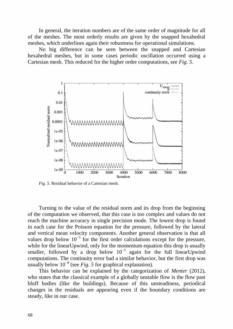
68

In general, the iteration numbers are of the same order of magnitude for all

of the meshes. The most orderly results are given by the snapped hexahedral

meshes, which underlines again their robustness for operational simulations.

No big difference can be seen between the snapped and Cartesian

hexahedral meshes, but in some cases periodic oscillation occurred using a

Cartesian mesh. This reduced for the higher order computations, see Fig. 5.

Fig. 5. Residual behavior of a Cartesian mesh.

Turning to the value of the residual norm and its drop from the beginning

of the computation we observed, that this case is too complex and values do not

reach the machine accuracy in single precision mode. The lowest drop is found

in each case for the Poisson equation for the pressure, followed by the lateral

and vertical mean velocity components. Another general observation is that all

values drop below 10−5

for the first order calculations except for the pressure,

while for the linearUpwind, only for the momentum equation this drop is usually

smaller, followed by a drop below 10−5

again for the full linearUpwind

computations. The continuity error had a similar behavior, but the first drop was

usually below 10−8

(see Fig. 5 for graphical explanation).

This behavior can be explained by the categorization of Menter (2012),

who states that the classical example of a globally unstable flow is the flow past

bluff bodies (like the buildings). Because of this unsteadiness, periodical

changes in the residuals are appearing even if the boundary conditions are

steady, like in our case.

69

3.3. Computational cost analysis

One of the main goals of the paper is to compare the models from a regulatory

purpose point of view. When carrying out simulations for, e.g., a government, it

is usually not possible to wait several days until the simulation is finished on a

cluster, and stability is of high importance. For this reason, the computational

costs are also evaluated.

The results of this analysis for all of the meshes can be seen in Fig. 6. It is

apparent, that the memory usage scales linearly for all of the meshes, and the

difference in the mesh types can be explained by the relative number of cell

faces, i.e., the polyhedral mesh uses more memory for a given number of cells,

while the tetrahedral mesh uses less. There is no significant difference between

the two kinds of hexahedral meshes, but it is important to note that the solver

itself takes no benefit from the fact that one of them is Cartesian.

Fig. 6. Computational cost of the simulations for the full upwind simulations, 4000

iterations.

For the comparison of the CPU time, only the relative values are

interesting, and it can be seen that the CPU time demand scales linearly with the

number of cells, and there is no significant difference in the mesh types. These

comparative simulations were carried out on the new cluster of the University of

Siegen (http://www.uni-siegen.de/cluster/index.html?lang=en), run for 4000

iterations with first order upwinding for all variables on 24 cores. As a rule of

thumb for this setup it can be said, that a simulation result can be obtained in

70

1 hour/1 million cells. Those meshes which were unstable with the default

relaxation factors are omitted from the CPU-time graph.

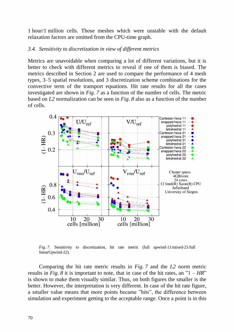
3.4. Sensitivity to discretization in view of different metrics

Metrics are unavoidable when comparing a lot of different variations, but it is

better to check with different metrics to reveal if one of them is biased. The

metrics described in Section 2 are used to compare the performance of 4 mesh

types, 3–5 spatial resolutions, and 3 discretization scheme combinations for the

convective term of the transport equations. Hit rate results for all the cases

investigated are shown in Fig. 7 as a function of the number of cells. The metric

based on L2 normalization can be seen in Fig. 8 also as a function of the number

of cells.

Fig. 7. Sensitivity to discretization, hit rate metric (full upwind-11/mixed-21/full linearUpwind-22).

Comparing the hit rate metric results in Fig. 7 and the L2 norm metric

results in Fig. 8 it is important to note, that in case of the hit rates, an ‖1 – HR‖

is shown to make them visually similar. Thus, on both figures the smaller is the

better. However, the interpretation is very different. In case of the hit rate figure,

a smaller value means that more points became ‖hits‖, the difference between

simulation and experiment getting to the acceptable range. Once a point is in this

71

range, the hit rate will not improve even if the results get closer to each other.

On the other hand, for the L2 norm metric, a smaller value means that the

difference between simulation and experiment got smaller.

Fig. 8. Sensitivity to discretization, L2 metric (full upwind-11/mixed-21/full

linearUpwind-22).

For the absolute value of the hit rate metric for the mean velocity values it

can be said, that these high hit rates are good results for this complex case.

Similar values were found by Efthimiou et al. (2011) for two other codes,

Andrea® and Star-CD

®, and by Franke et al. (2012b) and Rakai and Franke

(2012) for the ANSYS® Fluent code for the mean velocities. No further exact

comments can be made for the turbulent quantities, as the threshold value was

chosen arbitrarily and not based on measurement uncertainties. In the VDI

guideline (VDI, 2005) an acceptable HR value is given for certain test cases,

thresholds, and measurement points, but it is not easily transferable to a totally

different case.

The absolute value of the L2 norm metrics can be interpreted as a kind of

relative error, showing that for the streamwise velocity results, where the values

are essentially higher, the metric is smaller than for all the other variables. For

the conclusions drawn later, the absolute value of this metric is not considered.

The conclusions which can be drawn from Fig. 8 of the L2 metric norm are

the following:

72

1. For streamwise velocities, tetrahedral meshes perform outstandingly better.

From theoretical point of view, the smallest numerical error is expected

from the hexahedral meshes. The reason for this is shown by Juretic and

Gosman (2010): because the hexahedral mesh is aligned with the flow, the

errors in fluxes cancel. Explanation for the superior performance of the same

mesh size for the tetrahedral meshes in this case can be that those were made

with the Delauney algorithm, so they are not ―wasting‖ so many cells in the

middle of the domain where there is no geometric feature to disturb the flow, so

the gradients are small and do not make high mesh resolution necessary. In case

of the hexahedral meshes, the underlying original mesh block has a quite high

density. This can be seen in the two coarse meshes compared in Fig 9. It is also

seen that the transition of tetrahedral cells is smoother from the fine to the coarse

cells, and above the canopy where there are still strong gradients, the hexahedral

meshes are not resolved enough. See Fig. 10 for the visualization of these

gradients above the urban canopy. A line is shown in Fig. 9 below which high

gradients occur in the solution.

Franke et al. (2012b) used also a block-structured hexahedral mesh for

their investigations with ANSYS® Fluent and had better performance also in the

mean velocities. That mesh is not automatically generated and has very different

mesh quality metrics than the automatic snappyHexMesh meshes (average non-

orthogonality 2.64, maximum skewness 1.47, and smooth cell volume

transition). The worse results of the automatic hexahedral meshes can be

explained by their larger and lower quality cells in the most important regions

shown in Fig. 9.

Fig. 9. Tetrahedral (6.65 ×106 cells) and hexahedral (8.0 ×10

6 cells) mesh cross sections

(diagonal lines are just visualization tool specific features in the hexahedral mesh).

73

Fig. 10. Profile 29 of one tetrahedral (6.65 ×106) and one hexahedral (8.0 ×10

6) mesh

(full linearUpwind solution).

2. Better performance of the tetrahedral meshes is not so apparent for lateral

velocity, and disappears for the rms values.

To better understand this phenomenon, Fig. 10 shows the profiles

compared at location 29 (see Fig. 1) which is in the yard of an 18 m high

building. In the non-dimensional scale 0.18 is the top of the building and it can

be observed that changes in streamwise mean velocity reach 0.4, while for the

other values the maximum is 0.3. So the smoother transition of the tetra mesh

can help to better resolve the streamwise velocity, but for the other values it is

not so important. The oscillations on the profiles for the tetra meshes can be

found on other profiles computed with OpenFOAM® as well. They may be a

consequence of the instability of the simulations, however, for the ANSYS®

Fluent results they do not appear. This phenomenon needs further investigation.

3. Full second order solutions perform better already for the mean values, but

that difference competes with the CPU-time cost of the results. For the

turbulent quantities, however, full second order solutions are outstanding.

Theoretically this is obvious as higher order terms are more accurate, but

on the other hand, this can amplify the errors in the modeling assumptions. In

the Michel-Stadt case the higher order results for the simulation always compare

better to the experimental values. It must be kept in mind that not all

74

micrometeorological models use higher order advective terms. As the turbulent

quantities are used for the dispersion calculations, it can have a significant effect

and higher order terms are suggested.

4. Polyhedral meshes have very low performance compared to all the other

cases if not full second order discretization is used.

This can be a result of the larger volumes in those meshes and the large cell

volume changes explained, strengthening the numerical errors. It is suggested to

use polyhedral meshes only with higher order convective/advective terms, as

those metrics are comparable with the other mesh types.

5. The Cartesian hexahedral meshes have lower performance in the mean

velocities, but this disappears for the turbulent statistics.

More comparable results for rms value prediction need further

investigation. This can be caused by the generally wrong rms predictions for all

mesh types and by the numerical errors canceling the modeling errors.

6. There is a jump of low performance for the second coarsest hexahedral

meshes which is visible both in the hit rate metric and L2 norm metric.

This is a sign that mesh refinement does not always lead to improved

solutions because of the error cancellation explained above. Also the importance

of investigation of mesh dependency on more meshes must be noted.

4. Conclusions and outlook

Sensitivity of four different metrics to compare experimental and simulation

results was investigated for a test case of an idealized Central European city

center, Michel-Stadt. The numerical discretization approaches were compared

with four different mesh types, at least 3 resolutions for each of them, and

different discretization procedures of the convective/advective term in a

numerical experiment.

It was found that snappyHexMesh meshes are more stable computationally.

so they are more appropriate for operational purposes, although their metric

performance is not as good as that of the tetrahedral meshes. The lower

validation metric performance is not true in general for all hexahedral meshes,

more time consuming block-structured meshes with higher mesh quality metrics

can be generated which are both stable and more accurate.

For diagonal components of the Reynolds stresses, i.e., the rms values in

experimental results, discretization schemes of the convective terms have a

striking but expectable effect which must be kept in mind for dispersion studies

where their value effects turbulent diffusion. Numerical discretization

differences can cause almost 20 % change in the hit rate metric.

75

There are still many open questions to be further investigated, e.g., the

oscillation in the tetrahedral profiles, correspondence between stability and mesh

quality of the different mesh types, and the generation of the polyhedral mesh to

explain their low upwind validation metrics. This will be carried out through

further more detailed analyses of the datasets.

The work with Michel-Stadt continues in the framework of COST Action

ES 1006 with numerical uncertainty estimation and dispersion studies for

continuous and puff passive scalar sources. The Action involves several research

groups who use different codes, including prognostic microscale obstacle

resolving meteorological models, diagnostic flow models, and operational

Gaussian type plume models. After investigations of the setup shown in this

paper, a blind test will be carried out to evaluate the use of local-scale

emergency prediction and response tools for airborne hazards in built

environments.

Acknowledgement–This research was financed by a scholarship of the Hungarian Government and the

project Talent Care and Cultivation in the Scientific Workshops of BME. The project is supported by

the grant TAMOP-4.2.2/B-10/1-2010-0009. It is also related to the scientific programme of the project

Development of Quality-Oriented and Harmonized R+D+I Strategy and the Functional Model at

BME, the New Hungary Development Plan (Project ID: TAMOP-4.2.1/B-09/1/KMR-2010-0002), and

the K 108936 ID project of the Hungarian Scientific Research Fund. Collaboration of the authors was

possible thanks to two DAAD (German Academic Exchange Service) research grants, number

A/10/82525 and A/11/83345.

References

Ansys®, 2009: Ansys Fluent 14.0 Theory Guide. Canonsburg, Pennsylvania.

Baklanov, A. and Nuterman, R.B., 2009: Multi-scale atmospheric environment modelling for urban

areas. Adv. Sci. Res. 3, 53–57.

Baklanov, A., 2000: Application of CFD methods for modelling in air pollution problems: possibilities

and gaps. Environ. Monit. Assess. 65, 181–189.

Balczó, M., Balogh, M., Goricsan, I., Nagel, T., Suda, J., and Lajos, T., 2011: Air quality around

motorway tunnels in complex terrain – computational fluid dynamics modeling and comparison

to wind tunnel data. Időjárás 115, 179–204.

Balogh, M., Parente, A., and Benocci, C., 2012: RANS simulation of ABL flow over complex terrains

applying an Enhanced k-ε model and wall function formulation: Implementation and

comparison for fluent and OpenFOAM®. J. Wind Eng. Ind. Aerod. 104–106, 360–368.

Blocken, B., Stathopoulos, T., and Carmeliet, J., 2007a: CFD evaluation of wind speed conditions in

passages between parallel buildings – effect of wall-function roughness modifications for the

atmospheric boundary layer flow. J. Wind Eng. Ind. Aerod. 95, 941–962.

Blocken, B., Stathopoulos, T., and Carmeliet, J., 2007b: CFD simulation of the atmospheric boundary

layer: wall function problems. Atmos. Environ. 41, 238–252.

Britter, R.E. and Hanna, S.R., 2003: Flow and dispersion in urban areas. Annu. Rev. Fluid Mech. 35,

469–96.

COST ES1006, 2012: COST ES1006 Background and Justification Document. COST. Action ES 1006:

Evaluation, improvement and guidance for the use of local-scale emergency prediction and

response tools for airborne hazards in built environments.

Durbin, P.A., 1996: On the k- ε stagnation point anomaly. Int. J. Heat Fluid Flow 17, 89–90.

76

Eca, L. and Hoekstra, M., 2008: Testing Uncertainty Estimation and Validation Procedures in the

Flow Around a Backward Facing Step. In Proceedings of the 3rd Workshop on CFD

Uncertainty Analysis.

Efthimiou, G.C., Hertwig, D., Fischer, R., Harms, F., Bastigkeit, I., Koutsourakis, N., Theodoridis, A.,

Bartzis, J.G., and Leitl, B., 2011: Wind flow validation for individual exposure studies. In

Proceedings of the 13th International Conference on Wind Engineering (ICWE13), Amsterdam,

The Netherlands.

Ehrhard, J., Kunz, R., and Moussiopoulos, N., 2000: On the performance and applicability of

nonlinear two equation turbulence models for urban air quality modelling. Environ. Monit.

Assess. 65, 201–209.

Eichhorn, Dr. J., 2008: MISKAM manual for version 5. Spielplatz 2 55263 Wackernheim.

ERCOFTAC, 2000: Best Practice Guidelines. ERCOFTAC Special Interest Group on“Quality and

Trust in Industrial CFD”.

Ferziger, J.H. and Peric, M., 2002: Computational Methods for Fluid Dynamics. Springer, Berlin

Heidelberg New-York

Fischer, R., Bastigkeit, I., Leitl, B., and Schatzmann, M., 2010: Generation of spatio-temporally high

resolved datasets for the validation of LES- models simulating flow and dispersion phenomena

within the lower atmospheric boundary layer. In Proceedings of The Fifth International

Symposium on Computational Wind Engineering (CWE2010), Chapel Hill, North Carolina,

USA.

Franke, J., Hellsten, A., Schlünzen, H., and Carissimo, B., 2007: Best Practice Guideline for the CFD

Simulation of Flows in the Urban Environment. COST Action 732: Quality Assurance and

Improvement of Microscale Meteorological Models.

Franke, J., 2010: A review of verification and validation in relation to CWE. In Proceedings of the

Fifth International Symposium on Computational Wind Engineering (CWE2010) Chapel Hill,

North Carolina, USA, May 23–27, 2010.

Franke, J., Hellsten, A., Schlunzen, K.H., and Carissimo, B. 2011. 2011 The COST 732 Best Practice

Guideline for CFD simulation of flows in the urban environment: a summary. International

Journal of Environment and Pollution, 44(1–4), 419–427.

Franke, J., Sturm, M., and Kalmbach, C., 2012a: Validation of OpenFOAM® 1.6.x with the German

VDI guideline for obstacle resolving microscale models. J. Wind Eng. Ind. Aerod. 104–106,

350–359.

Franke, J., Laaser, A., Bieker, B., and Kempfer, T. 2012b: Sensitivity analysis of RANS simulations

for flow and dispersion in the generic European City Centre Michel-Stadt. In Proceedings of

Conference on Modelling Fluid Flow. Budapest, Hungary, Sept 4–7 2012.

Hefny, M.M. and Ooka, R., 2009: CFD analysis of pollutant dispersion around buildings: Effect of cell

geometry. J. Build. Environ. 44, 1699–1706.

Janssen, W.D, Blocken, B., and van Hoof, T. 2012: Pedestrian wind comfort around buildings:

comparison of wind comfort criteria based on whole-flow field data for a complex case study. J.

Build. Environ. accepted for publication.

Jasak, H., 1996: Error Analysis and Estimation for the Finite Volume Method with Application to

Fluid Flows. PhD. Thesis, Imperial College of Science, Technology and Medicine.

Juretic, F. and Gosman, A.D., 2010: Error Analysis of the Finite-Volume Method with respect to

Mesh Type. Num. Heat Transfer 57, 414–439.

Leelőssy, Á., 2012: Baleseti kibocsátásból származó szennyezőanyagok lokális skálájú terjedésének

modellezése. M.Sc. thesis, Eötvös Lóránd Univ. Dep. Meteorology. (In Hungarian)

Lun, Y.F., Mochida, A., Murakami, S., Yoshino, H., and Shirasawa, T., 2003: Numerical simulation of

flow over topographic features by revised k − ε models. J. Wind Eng. Ind. Aerod. 91, 231–245.

Menter, F.R., 2012: Best Practice: Scale-Resolving Simulations in ANSYS® CFD. ANSYS

®, Germany.

Mészáros, R., Vincze, Cs., and Lagzi, I., 2010: Simulation of accidental release using a coupled

transport (TREX) and numerical weather prediction (ALADIN) model. Időjárás 114, 101–120.

Oberkampf, W.L., and Trucano, T.G., 2002: Verification and validation in computational fluid

dynamics. Prog. Aerospace Sci, 38. 209–272.

OpenCFD Limited, 2011: OpenFOAM® User Guide – Version 2.0.0. OpenCFD Limited.

77

O’Sullivan, J.P., Archer, R.A., and Flay, G.J., 2011: Consistent boundary conditions for flows within

the atmospheric boundary layer. J. Wind Eng. Ind. Aerod. 99, 65–77.

Parente, A., Gorlé, C., van Beeck, J., and Benocci, C. 2010: A Comprehensive Modelling Approach

for the Neutral Atmospheric Boundary Layer: Consistent Inflow Conditions, Wall Function and

Turbulence Model. Bound-Lay. Meteorol. 140, 411–428.

Rakai, A. and Franke, J., 2012: Validation of two RANS solvers with flow data of the flat roof

Michel-Stadt case. In Proc. 8th International Conference on Air Quality – Science and

Application, Athens, Greece.

Rakai, A., and Kristóf, G., 2010: CFD Simulation of Flow over a Mock Urban Setting Using

OpenFOAM®. In Gépészet 2010: Proceedings of the Seventh Conference on Mechanical

Engineering. Budapest, Hungary.

Richards, P.J. and Hoxey, R., 1993: Appropriate boundary conditions for computational wind

engineering models using the k − turbulence model. J. Wind Eng. Ind. Aerod. 47, 145–153.

Roache, P.J., 1997: Quantification of Uncertainty in Computational Fluid Dynamics. Annu. Rev. Fluid

Mech. 29, 123–60.

Schatzmann, M., Olesen, H., and Franke, J. 2009: COST 732 Model Evaluation Case Studies:

Approach and Results. COST Action 732: Quality Assurance and Improvement of Microscale

Meteorological Models.

Schatzmann, M. and Leitl, B., 2011: Issues with validation of urban flow and dispersion CFD models.

J. Wind Eng. Ind. Aerod. 99, 169–186.

Stull, R.B., 1988: An Introduction to Boundary Layer Meteorology. Kluwer Academic Pub.

Tominaga, Y., Mochida, A., Yoshie, R., Kataoka, H., Nozu, T,, Kazuyoshi, Y,, M., and Shirasawa, T.,

2008: AIJ guidelines for practical applications of CFD to pedestrian wind environment around

buildings . J. Wind Eng. Ind. Aerod. 96, 1749–1761.

Tominaga, Y., Mochida, A., Shirasawa, T., Yoshie, R., Kataoka, H., Harimoto, K., and Nozu, T., 2004:

Cross Comparison of CFD Results of Wind Environment at Pedestrian Level around a High-rise

Building and within a Building Complex. J. Asian Arch. Build. Engin., 3.

VDI., 2005: Environmental Meteorology – Prognostic microscale wind field models – Evaluation for

flow around buildings and obstacles, VDI guideline 3783, Part 9.

Wright, N.G., and Easom, G.J., 2003: Non-linear k − turbulence model results for flow over a building

at full scale. Appl. Math. model. 27, 1013–1033.

Yang, Y., Gu, M., Chen, S., and Jin, X., 2007: New inflow boundary conditions for modeling the

neutral equilibrium atmospheric boundary layer in computational wind engineering. J. Wind

Eng. Ind. Aerod. 97, 88–95.

Yoshie, R., Mochida, A., Tominaga, Y., Kataoka, H., and Yoshikawa, M., 2005: Cross Comparison of

CFD Prediction for Wind Environment at Pedestrian Level around Buildings Part 1-2. In

Proceedings of the 6th Asia-Pacific Conference on Wind Engineering (APCWE-VI).Seoul, Korea,

September 12–14, 2005.