PDF (189 KB)
26
LETTER Communicated by Nigel Goddard Advancing the Boundaries of High-Connectivity Network Simulation with Distributed Computing Abigail Morrison [email protected] Computational Neurophysics, Institute of Biology III and Bernstein Center for Computational Neuroscience, Albert-Ludwigs-University, 79104 Freiburg, Germany Carsten Mehring [email protected] Department of Zoology, Institute of Biology I and Berstein Center for Computational Neuroscience, Albert-Ludwigs-University, 79104 Freiburg, Germany Theo Geisel [email protected] Department of Nonlinear Dynamics, Max-Planck-Institute for Dynamics and Self Organization, 37018 G¨ ottingen, Germany Ad Aertsen [email protected] Neurobiology and Biophysics, Institute of Biology III and Bernstein Center for Computational Neuroscience, Albert-Ludwigs-University, 79104 Freiburg, Germany Markus Diesmann [email protected] Computational Neurophysics, Institute of Biology III and Bernstein Center for Computational Neuroscience, Albert-Ludwigs-University, 79104 Freiburg, Germany The availability of efficient and reliable simulation tools is one of the mission-critical technologies in the fast-moving field of computational neuroscience. Research indicates that higher brain functions emerge from large and complex cortical networks and their interactions. The large number of elements (neurons) combined with the high connectivity (synapses) of the biological network and the specific type of interactions impose severe constraints on the explorable system size that previously have been hard to overcome. Here we present a collection of new tech- niques combined to a coherent simulation tool removing the fundamen- tal obstacle in the computational study of biological neural networks: the enormous number of synaptic contacts per neuron. Distributing an individual simulation over multiple computers enables the investigation of networks orders of magnitude larger than previously possible. The Neural Computation 17, 1776–1801 (2005) © 2005 Massachusetts Institute of Technology
Transcript of PDF (189 KB)
LETTER Communicated by Nigel Goddard
Advancing the Boundaries of High-Connectivity NetworkSimulation with Distributed Computing
Abigail [email protected] Neurophysics, Institute of Biology III and Bernstein Center forComputational Neuroscience, Albert-Ludwigs-University, 79104 Freiburg, Germany
Carsten [email protected] of Zoology, Institute of Biology I and Berstein Center for ComputationalNeuroscience, Albert-Ludwigs-University, 79104 Freiburg, Germany
Theo [email protected] of Nonlinear Dynamics, Max-Planck-Institute for Dynamics and SelfOrganization, 37018 Gottingen, Germany
Ad [email protected] and Biophysics, Institute of Biology III and Bernstein Center forComputational Neuroscience, Albert-Ludwigs-University, 79104 Freiburg, Germany
Markus [email protected] Neurophysics, Institute of Biology III and Bernstein Center forComputational Neuroscience, Albert-Ludwigs-University, 79104 Freiburg, Germany
The availability of efficient and reliable simulation tools is one of themission-critical technologies in the fast-moving field of computationalneuroscience. Research indicates that higher brain functions emerge fromlarge and complex cortical networks and their interactions. The largenumber of elements (neurons) combined with the high connectivity(synapses) of the biological network and the specific type of interactionsimpose severe constraints on the explorable system size that previouslyhave been hard to overcome. Here we present a collection of new tech-niques combined to a coherent simulation tool removing the fundamen-tal obstacle in the computational study of biological neural networks:the enormous number of synaptic contacts per neuron. Distributing anindividual simulation over multiple computers enables the investigationof networks orders of magnitude larger than previously possible. The
Neural Computation 17, 1776–1801 (2005) © 2005 Massachusetts Institute of Technology
Distributed High-Connectivity Network Simulation 1777
software scales excellently on a wide range of tested hardware, so it can beused in an interactive and iterative fashion for the development of ideas,and results can be produced quickly even for very large networks. In con-trast to earlier approaches, a wide class of neuron models and synapticdynamics can be represented.
1 Introduction
It has long been pointed out (Hebb, 1949; Braitenberg, 1978) that cortical pro-cessing is most likely carried out by large ensembles (assemblies) of nervecells, whereby the membership of neurons in various assemblies is exhib-ited through the complex correlation structure of their spike trains (vonder Malsburg, 1981, 1986; Abeles, 1982, 1991; Palm, 1990; Aertsen, Gerstein,Habib, & Palm, 1989; Gerstein, Bedenbaugh, & Aertsen, 1989; Singer, 1993,1999). Theoretical studies (Shadlen & Newsome, 1998; Diesmann, Gewaltig,& Aertsen, 1999; Salinas & Sejnowski, 2000; Kuhn, Aertsen, & Rotter, 2003)have demonstrated that the cortical neuron is indeed sensitive to the higher-order correlation structure of their input. With the experimental technologyfor multiple-single unit recordings becoming routinely available for ani-mals involved in behavioral tasks, appropriate network models need to beconstructed to interpret the results.
Due to the nonlinear and stochastic nature of neural systems, simulationshave become a research tool of major importance in the developing field ofcomputational neuroscience (Dayan & Abbott, 2001; Koch, 1999; Koch &Segev, 1989). A number of simulation tools have been developed (Genesis:Bower & Beeman, 1997; Neuron: Hines & Carnevale, 1997; XPP: Ermentrout,2002) and are in widespread use. They are general purpose in the sensethat they maintain a layer of abstraction between the neuron model to besimulated and the machinery implementing the network interaction; thatis, they are not neuron or network model specific. The primary focus ofthese tools is small networks of detailed neuron models. One exception isSpikeNET (Delorme & Thorpe, 2003), which is specialized for a specific classof large networks of spiking neurons.
A major barrier in the simulation of mammalian cortical networks hasbeen the large number of inputs (afferents) a single neuron receives. As-suming a biologically realistic level of connectivity, each neuron shouldhave of the order of 104 afferents. In order to ensure that the network issufficiently sparse, a connection probability of 0.1 should be assumed, re-sulting in a minimal network size of 105 neurons, corresponding to roughlya cubic millimeter of cortex (Braitenberg & Schuz, 1998). Such a networkcontains of the order of 109 synapses and has proved to be beyond thememory capacity of the computers available to many researchers. Fur-thermore, even given a computer with sufficient memory resources, theamount of time required to construct and simulate such networks and
1778 A. Morrison, C. Mehring, T. Geisel, A. Aertsen, and M. Diesmann
perform reasonable parameter scans is not conducive to rapid scientificprogress.
Faced with these problems, many researchers have opted to use scalednetworks, in which the connection probability remains constant and thesynaptic weights are scaled in some manner with the inverse of the totalnumber of connections a neuron receives. This approach is not withoutits risks; although the mean or, alternatively, the standard deviation of thesubthreshold activity can be held constant, this is not true for correlationsand combinatorial measures. Furthermore, in such networks, the memoryrequirement increases quadratically with the number of neurons. Clearly,these disadvantages hold only until the minimal network size is attained,at which point synaptic scaling need no longer be applied and memoryrequirements increase only linearly with increasing network size.
In this letter, we describe without reference to a particular implemen-tation language how distributed computing (i.e., simultaneous executionon multiple processors, where the addressable memory of one processor isnot visible to the others) can be used to acquire the memory resources tosurpass the threshold of 105 neurons and reach a simulation speed suitablefor practical work.
To our knowledge, this is the first description of a general-purpose sim-ulation scheme that allows the routine investigation of networks of spikingneurons with biologically realistic levels of connectivity. Our design consistsof a highly efficient distributed algorithm, based on the serial (i.e., runningon one processor) simulation kernel first described in Diesmann, Gewaltig,and Aertsen (1995). Despite the use of a distributed algorithm, a serial inter-face is presented to the researcher. In addition to the increases in network sizeand simulation speed enabled by our approach, a key feature of our designis its flexibility due to object orientation (the implementation language be-ing C++; Stroustrup, 1997). Recent advances in simulation technique havetended to focus on current-based integrate-and-fire point neurons (Mattia &Del Giudice, 2000; Lee & Farhat, 2001; Reutimann, Giugliano, & Fusi, 2003);using our technology, the researcher is not bound by any of these restrictionsand can just as easily use conductance-based neurons (e.g., Chance, Abbott,& Reyes, 2002; Destexhe, Rudolph, & Pare, 2003; Kuhn, Aertsen, & Rotter,2004), non-integrate-and-fire models (Hawkes, 1971), simple compartment-based models (Larkum, Zhu, & Sakmann, 2001; Kumar, Kremkow, Rotter,& Aertsen, 2004), or implement a neuron model of his or her own. Whereascomplex compartmental models could theoretically be implemented, thereis no support for generating them as in Neuron (Hines & Carnevale, 1997)or Genesis (Bower & Beeman, 1997), and so such models remain out ofthe reach of the current version. The main constraint is the restriction to theclass of neuron models where the interaction between neurons is noninstan-taneous (finite delays) and mediated by point events (spikes). Similarly, alarge range of synaptic dynamics can be employed, and a network may beentirely heterogeneous in terms of the neuron and synapse models used.
Distributed High-Connectivity Network Simulation 1779
In section 2, we describe the representation and construction of a net-work, including compression techniques. On this basis, we explain thedistributed algorithm for solving the dynamics in section 3. After a briefdiscussion of the treatment of pseudorandom numbers in section 4, we pro-vide benchmarks for our simulation technology in section 5 using relevantsimulation examples and hardware, demonstrating its excellent scalabilitywith respect to number of processors, network activity, and network sizeon computer clusters and parallel computers (for the purpose of this arti-cle, we reserve the term parallel computer for shared memory architectures).Section 6 summarizes the key concepts of our simulation scheme and dis-cusses our approach in the light of future directions of neuroscience researchand upcoming computer architectures.
Source code detail is out of the scope of this letter, as is simulation in-frastructure such as writing data to files. In the following, the term machinerefers to one processor, addressing memory that is assumed to be invisi-ble by other machines. Thus, a computer with two processors and sharedmemory would be regarded as two machines. The term list is taken in itsintuitive meaning of a sequential ordering, which need not necessarily beimplemented as the data structure known as list (Aho, Hopcroft, & Ullman,1983).
The research on a distributed simulation kernel described in this article isa module in our long-term collaborative project to provide the technologyfor neural systems simulations (Diesmann & Gewaltig, 2002). The appli-cation of the technology described here has already enabled interesting in-sights into the nature of cortical dynamics (Mehring, Hehl, Kubo, Diesmann,& Aertsen, 2003; Aviel, Mehring, Abeles, & Horn, 2003; Tetzlaff, Morrison,Geisel, & Diesmann, 2004).
Preliminary results have been presented in abstract form (Morrison et al.,2003).
2 Representation of Network Structure
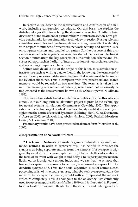
2.1 A Generic Network. Consider a generic network of spiking pointmodel neurons. In order to represent this, it is helpful to consider thesynapses as being separate entities from the neurons. If a synapse is trig-gered by a spike from its presynaptic neuron, it transmits this information inthe form of an event with weight w and delay d to its postsynaptic neuron.Each neuron is assigned a unique index, and we say that the synapse thattransmits a spike from neuron i to neuron j is an axonal synapse of i but adendritic synapse of j . Thus, for a serial algorithm, a list of neurons, eachpossessing a list of its axonal synapses, whereby each synapse contains theindex of its postsynaptic neuron, would suffice to represent the networkstructure completely. This is analogous to the adjacency lists commonlyused to represent graphs (Gross & Yellen, 1999) and is illustrated in Figure 1.Inorder to allow maximum flexibility in the structure and heterogeneity of
1780 A. Morrison, C. Mehring, T. Geisel, A. Aertsen, and M. Diesmann
VIτ
Index: 12
wd
Index: 7
1 23
45
6
12
7
9
11
8
123456789
1112
10
4
31 2 7
83 595
9786
21
5 6 10
12
11
10
SynapsesNeurons
10
Figure 1: Data structures for a serial simulation scheme. The network comprisesN uniquely indexed neurons (left column), and each neuron is assigned a list ofaxonal synapses (right column). Each neuron contains its own state variables, asdoes each synapse (illustrated by close-up). In addition, each synapse containsthe index of its postsynaptic neuron.
the networks that can be simulated, an object-oriented approach is highlyadvantageous, in which each individual neuron and synapse maintains itsown parameters, as depicted in the close-up in Figure 1, and performs itsown dynamics rather than being subject to a global algorithm.
For a distributed algorithm, matters are somewhat more complicated.The most obvious requirement for distributing a simulation is that the neu-rons are distributed. The simplest possible load balancing is to assign anequal number of neurons to each machine. As there may be different neu-ron models with different associated computational costs in the network,this assignment is performed using a modulo operation, so that contiguousblocks of neurons (the most intuitive way of defining neuron populations)are dealt out among all the machines, resulting in a good estimate of thefairest load distribution. For simplicity, here and in the remainder of the ar-ticle, we ignore this assignment and assume that neurons 1 to N/m, wherem is the number of machines, are located on the first machine, neuronsN/m + 1 to 2N/m on the second machine, and so on. Clearly, the synapsesmust also be distributed. We distribute the axonal synapses of each neuronas follows: on each machine, there are N lists of synapses, one for each neu-ron in the network. A synapse from neuron i to neuron j is stored in the ithlist on the machine owning neuron j . Alternatively, from a biological pointof view, we say the axon of a neuron is distributed, but its dendrite is local,as anticipated in Mattia and Del Giudice (2000). This seems less intuitivethan distributing the dendrite and keeping the axon local, but confers aconsiderable advantage in communication costs, as discussed in section 3.
Distributed High-Connectivity Network Simulation 1781
NeuronsSynapses Machines
65
2153
123456
aaaaaa
b
b
12
1
1 23
45
68
1210
7
9
11
10
1211
987
NeuronsSynapses Machines
bba b
baba b
1
1298
10
789
11
7
10 12
4
2
3
56
1
Machine: bMachine: a
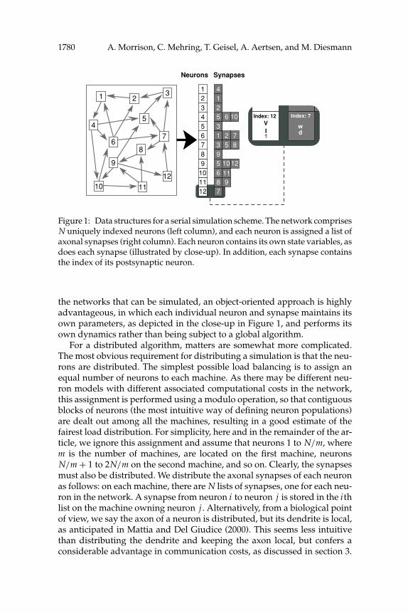
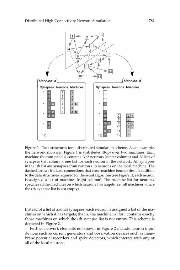
Figure 2: Data structures for a distributed simulation scheme. As an example,the network shown in Figure 1 is distributed (top) over two machines. Eachmachine (bottom panels) contains N/2 neurons (center column) and N lists ofsynapses (left column), one list for each neuron in the network. All synapsesin the ith list are synapses from neuron i to neurons on the local machine. Thedashed arrows indicate connections that cross machine boundaries. In additionto the data structures required for the serial algorithm (see Figure 1), each neuronis assigned a list of machines (right column). The machine list for neuron ispecifies all the machines on which neuron i has targets (i.e., all machines wherethe ith synapse list is not empty).
Instead of a list of axonal synapses, each neuron is assigned a list of the ma-chines on which it has targets; that is, the machine list for i contains exactlythose machines on which the ith synapse list is not empty. This scheme isdepicted in Figure 2.
Further network elements not shown in Figure 2 include neuron inputdevices such as current generators and observation devices such as mem-brane potential recorders and spike detectors, which interact with any orall of the local neurons.
1782 A. Morrison, C. Mehring, T. Geisel, A. Aertsen, and M. Diesmann
2.2 Network Construction. As the synapses are represented on the samemachine as their postsynaptic neuron, the network must also be connectedfrom the postsynaptic side: for each neuron, its afferent neurons must bespecified and a synapse added to the local synapse list of each of those neu-rons. Once the inputs for each neuron have been established, one completeexchange between the machines (see section 3.4) suffices to propagate theconnectivity information necessary to construct the machine list for eachneuron. Constructing the network is therefore a fully parallelizable activitythat results in a near-linear speed-up (see Figure 7). This is an importantfeature of our technology, as without parallelization, the wiring of a net-work can account for a large fraction of the total run time, especially asbiological levels of connectivity are approached. Despite the highly parallelnature of the construction, the user needs no knowledge about the locationof the neurons and can specify connections as if it were a serial applica-tion. On the most basic level, a command Connect(i, j) is ignored almostinstantaneously on all machines except the one owning neuron j . For higher-level connection commands, such as one for connecting a random network,we make use of the fact that a machine can determine at the beginning ofsuch a routine which neurons belong to it. The desired method can thenbe applied to all neurons within the appropriate bounds without having tocheck ownership of each neuron, thus achieving an even higher degree ofcode parallelization.
2.3 Network Compression. Simulations of large biological neural net-works are by their very nature highly consumptive of memory. Althoughthe emphasis of this article is on the use of distributed computing to providethe necessary memory resources, it is clear that any compression of the net-work structures will be beneficial, as it increases the size of network that canbe investigated on any given hardware and decreases the simulation timefor any given network. We therefore explain briefly the general principles ofhow redundancy can be reduced without special knowledge of the networkstructure in order to reduce the memory demands of a simulation.
We will consider the simplest synapse possible, a static synapse con-sisting of a constant weight w, a constant delay d, and the index of thepostsynaptic neuron i . Ignoring for simplicity the memory overhead in-volved in creating the synapse object, a naive representation of a synapsewould therefore require a number of bytes Ms = Mw + Md + Mi , and anetwork of N neurons with K synapses each would require NKMs bytespurely for the synapses. To give some idea of the scale of the problem, typ-ical values for Mw , Md , and Mi on a 32-bit system are 8, 4, and 4 bytes, re-spectively, and a network containing N = 105 neurons with a connectivity ofK = 104 synapses each would require 16 GB. However, instead of storing thepostsynaptic index for each synapse in a list, we keep the list sorted in orderof increasing index and store just the differences between them. If this dif-ference is less than 255, it can be stored in 1 byte. If the difference happens
Distributed High-Connectivity Network Simulation 1783
to be too large, an appropriate entry is made in an overflow list. In fact,in most applications, this is a rare occurrence. In the network mentionedabove, if connected using a uniform distribution, the average difference be-tween neurons is 10. If networks of orders of magnitude larger than thiswere to be investigated, spatial structure would have to be taken into con-sideration to avoid obtaining a biologically unrealistic sparseness. It shouldbe noted that the requirement of keeping the target lists sorted is fulfilledwithout extra costs if, given indices j1, j2 of neurons located on a particu-lar machine with j1 ≤ j2, the commands establishing the connections areissued in the sequence . . . , Connect(i1, j1), . . . , Connect(i2, j2), . . . the orderand location of the presynaptic neurons being irrelevant. This techniquereduces the amount of memory for each synapse to Ms � Mw + Md + 1.
Further compression can be achieved by considering the distributions ofthe synaptic delays and weights. In the best-case scenario, as far as memoryis concerned, each neuron makes only one kind of axonal synapse: wij = wi
and dij = di . In this case, the parameters have to be stored only once per listrather than once per synapse, resulting in Ms � 1 and reducing the memoryrequirements for the above example network to approximately 1 GB. In thenext best case, each neuron makes axonal synapses with weights and delaysthat take on only a few possible values (see, e.g., Brunel, 2000). Here, severalsynaptic lists will be initialized, one for each combination encountered. Thisproduces compression almost as good as in the ideal case. However, there isa non-negligible memory overhead associated with the construction of eachlist, so for a broad distribution of delays, it is more efficient to represent themin terms of their difference from a reference value. For many applications,this difference can be expressed in 1 byte, resulting in Ms � Mw + 1 + 1.Similar to the representation of the postsynaptic neurons, a value too faraway from the reference value can be stored in an overflow list. This kind ofcompression is applicable only to discrete-valued variables such as delay.There is currently no way to compress a continuous distribution.
These methods can be easily extended to more complicated synapse ob-jects, but the onus is on the user to be aware of the redundancies in thenetwork to be investigated and choose the appropriate kind of compres-sion. As illustrated above, depending on the heterogeneity of the network,eliminating redundancy can reduce the memory requirements significantly,so that even large networks can be simulated on hardware available to mod-est budgets. Conversely, with access to large clusters or parallel machines,it is possible to investigate networks orders of magnitude larger than pre-viously possible.
3 Simulation Dynamics
3.1 Time Driven or Event Driven? A Hybrid Approach to Simulation.The two classic approaches to simulation are time driven and event driven,also known as synchronous and asynchronous algorithms. We pursue a
1784 A. Morrison, C. Mehring, T. Geisel, A. Aertsen, and M. Diesmann
hybrid strategy whereby the neurons are updated at every time step, buta synapse is updated only if its presynaptic neuron produces a spike. Apurely event-driven algorithm such as that proposed by Mattia and DelGiudice (2000) is unsuitable for our purposes because it places too manyrestrictions on the classes of neurons that can be simulated. For exam-ple, any neuron class in which a spike induces a continuous postsynap-tic current would be very difficult to implement if a neuron is updatedonly on the arrival of a spike event. Furthermore, the motivation for thesealgorithms is the fact that the state of a current-based integrate-and-fire(IAF) neuron can be directly interpolated between events, where eventsare assumed to be rare. This perceived computational advantage dwindlesrapidly as the frequency of events increases: a neuron with 104 afferentconnections firing at just 1 Hz receives events at a rate of 10,000 Hz andis therefore at least as expensive to simulate event driven as on a timegrid with a step size of 0.1 ms. In Reutimann et al. (2003), a solution tothe problems of rise times and event saturation is presented for IAF neu-rons at the cost of large look-up tables and restrictions on the type of back-ground population activity. By updating the neurons in fixed time stepsand applying exact integration techniques where possible (Rotter & Dies-mann, 1999), we maintain a highly flexible simulation environment at nograve computational cost. As a consequence of this scheme, spike times areconstrained to the time grid and are expressed as multiples of h, the timestep or computational resolution. It should, however, be noted that a neu-ron can perform arbitary dynamics within this time step, including usingan internal resolution much finer than the one the spikes are constrainedto.
Conversely, a purely time-driven algorithm is equally unsuitable.Synapses are by far the most numerous elements in a network. This isthe case even when synaptic scaling is employed (i.e., using fewer butstronger synapses), but particularly so if biologically realistic connectiv-ity is assumed. Clearly, updating 109 synapses every time step would havecatastrophic consequences for simulation times. Fortunately, although theabove consideration that events are rare is not valid for neurons, it is validfor individual synapses—in the situation described above, a synapse pro-cesses events at just 1 Hz. Assuming that the synaptic state can be calculatedfrom its previous state, the time since its last update, and information avail-able from the postsynaptic neuron, a synapse need be updated only whenit transfers a spike event. In fact, a wide range of synaptic dynamics fallsinto this category, including synaptic depression (Thomson & Deuchars,1994), synaptic redistribution (Markram & Tsodyks, 1996), and spike-time-dependent plasticity (Bi & Poo, 1998, 2001), for a review see Abbott andNelson (2000).
By combining the flexibility of a time-driven algorithm with the speedof an event-driven algorithm, a highly functional and fast simulation envi-ronment is achieved.
Distributed High-Connectivity Network Simulation 1785
wt+h
rotation
y: state at t
y ←←
Fh(y)
y G(y, w t+h)
refractory?spike now?
refractory dynamicsspike
y: state at t + h
T
F
T
F
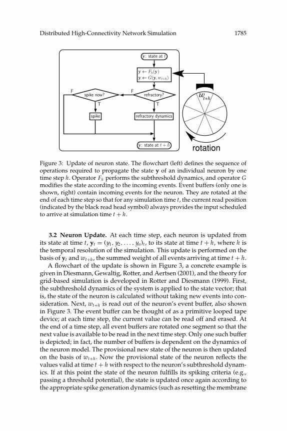
Figure 3: Update of neuron state. The flowchart (left) defines the sequence ofoperations required to propagate the state y of an individual neuron by onetime step h. Operator Fh performs the subthreshold dynamics, and operator Gmodifies the state according to the incoming events. Event buffers (only one isshown, right) contain incoming events for the neuron. They are rotated at theend of each time step so that for any simulation time t, the current read position(indicated by the black read head symbol) always provides the input scheduledto arrive at simulation time t + h.
3.2 Neuron Update. At each time step, each neuron is updated fromits state at time t, yt = (y1, y2, . . . , yn)t , to its state at time t + h, where h isthe temporal resolution of the simulation. This update is performed on thebasis of yt and wt+h , the summed weight of all events arriving at time t + h.
A flowchart of the update is shown in Figure 3, a concrete example isgiven in Diesmann, Gewaltig, Rotter, and Aertsen (2001), and the theory forgrid-based simulation is developed in Rotter and Diesmann (1999). First,the subthreshold dynamics of the system is applied to the state vector; thatis, the state of the neuron is calculated without taking new events into con-sideration. Next, wt+h is read out of the neuron’s event buffer, also shownin Figure 3. The event buffer can be thought of as a primitive looped tapedevice; at each time step, the current value can be read off and erased. Atthe end of a time step, all event buffers are rotated one segment so that thenext value is available to be read in the next time step. Only one such bufferis depicted; in fact, the number of buffers is dependent on the dynamics ofthe neuron model. The provisional new state of the neuron is then updatedon the basis of wt+h . Now the provisional state of the neuron reflects thevalues valid at time t + h with respect to the neuron’s subthreshold dynam-ics. If at this point the state of the neuron fulfills its spiking criteria (e.g.,passing a threshold potential), the state is updated once again according tothe appropriate spike generation dynamics (such as resetting the membrane

1786 A. Morrison, C. Mehring, T. Geisel, A. Aertsen, and M. Diesmann
potential). The emitted spike is assigned to the time t + h, and the informa-tion that it has occurred must be transmitted to the neuron’s distributedaxonal synapses. This calculation of the new state of the neuron is definedby the individual neuron model rather than by a global algorithm. In manycases, it is possible to avoid using computationally expensive differentialequation solvers by applying a propagator matrix to the neuron state tointegrate exactly (Rotter & Diesmann, 1999).
Clearly, the use of event buffers, already present in the original serialversion (Diesmann et al., 1995; Gewaltig, 2000), obviates the requirementfor a centralized event queuing system; an event of weight w due to arrive atthe neuron d time steps in the future can be added to the event buffer d stepsupstream from the current reading position. Obviously, causality requires anonzero transmission delay, that is, d ≥ 1. It is important to note the implicitassumption made here that the weights of incoming events can be summed,as each ring buffer segment contains just one value, which is incrementedby the weights of successive incoming events. It does not, however, implythat an incoming event may only cause a discontinuous jump in a statevariable of the neuron. The interpretation of the weights is left up to theindividual neuron model. For example, one model may interpret the weightsas the magnitude of a jump in the membrane potential and another as themaximum value of an alpha function (Jack, Noble, & Tsien, 1983; Bernard,Ge, Stockley, Willis, & Wheal, 1994) describing the change of conductance.Nor does it imply that all the events received by a neuron necessarily induceidentical dynamics. Models with different time constants for excitatory andinhibitory input, for example, or with several compartments (Kumar et al.,2004) are implemented by giving the neuron access to several such eventbuffers.
3.3 Index Buffering. At first glance it seems as if communication be-tween machines should take place after every time step in order to conveythe information of which neurons spiked during that time step. Fortunately,this is not so. If the minimum synaptic delay is dmin · h, then a neuron spik-ing at time t cannot have an effect on any postsynaptic neuron at a timeearlier than t + dmin · h. Therefore, if the spikes can be stored maintainingtheir temporal order, it is sufficient to communicate in intervals of dmin timesteps. This also represents the maximum possible communication interval;any greater communication interval would result in events arriving withdelays longer than those specified by the user. This communication schemeis completely independent of the temporal resolution; simulating on a finertime grid does not increase the frequency of communication. Maintainingthe temporal ordering is easily done. In each time step, the indices of allspiking neurons can be stored in a buffer as illustrated in Figure 4, and atthe end of the time step, a marker is inserted into the buffer to separatethe spikes of successive time steps. Note that if the axonal synapses werelocal and the dendritic synapses distributed, the synaptic weight, delay,
Distributed High-Connectivity Network Simulation 1787
123456
aaaaaa
b
b b6
Buffer for Machine:
a
Neurons Machines
Machine: a
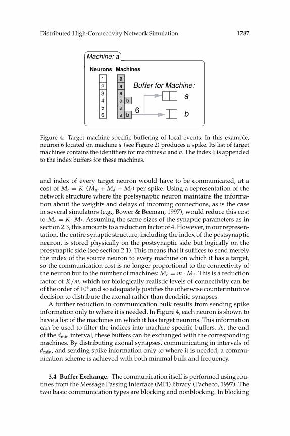
Figure 4: Target machine-specific buffering of local events. In this example,neuron 6 located on machine a (see Figure 2) produces a spike. Its list of targetmachines contains the identifiers for machines a and b. The index 6 is appendedto the index buffers for these machines.
and index of every target neuron would have to be communicated, at acost of Mc = K· (Mw + Md + Mi ) per spike. Using a representation of thenetwork structure where the postsynaptic neuron maintains the informa-tion about the weights and delays of incoming connections, as is the casein several simulators (e.g., Bower & Beeman, 1997), would reduce this costto Mc = K · Mi . Assuming the same sizes of the synaptic parameters as insection 2.3, this amounts to a reduction factor of 4. However, in our represen-tation, the entire synaptic structure, including the index of the postsynapticneuron, is stored physically on the postsynaptic side but logically on thepresynaptic side (see section 2.1). This means that it suffices to send merelythe index of the source neuron to every machine on which it has a target,so the communication cost is no longer proportional to the connectivity ofthe neuron but to the number of machines: Mc = m · Mi . This is a reductionfactor of K/m, which for biologically realistic levels of connectivity can beof the order of 104 and so adequately justifies the otherwise counterintuitivedecision to distribute the axonal rather than dendritic synapses.
A further reduction in communication bulk results from sending spikeinformation only to where it is needed. In Figure 4, each neuron is shown tohave a list of the machines on which it has target neurons. This informationcan be used to filter the indices into machine-specific buffers. At the endof the dmin interval, these buffers can be exchanged with the correspondingmachines. By distributing axonal synapses, communicating in intervals ofdmin, and sending spike information only to where it is needed, a commu-nication scheme is achieved with both minimal bulk and frequency.
3.4 Buffer Exchange. The communication itself is performed using rou-tines from the Message Passing Interface (MPI) library (Pacheco, 1997). Thetwo basic communication types are blocking and nonblocking. In blocking
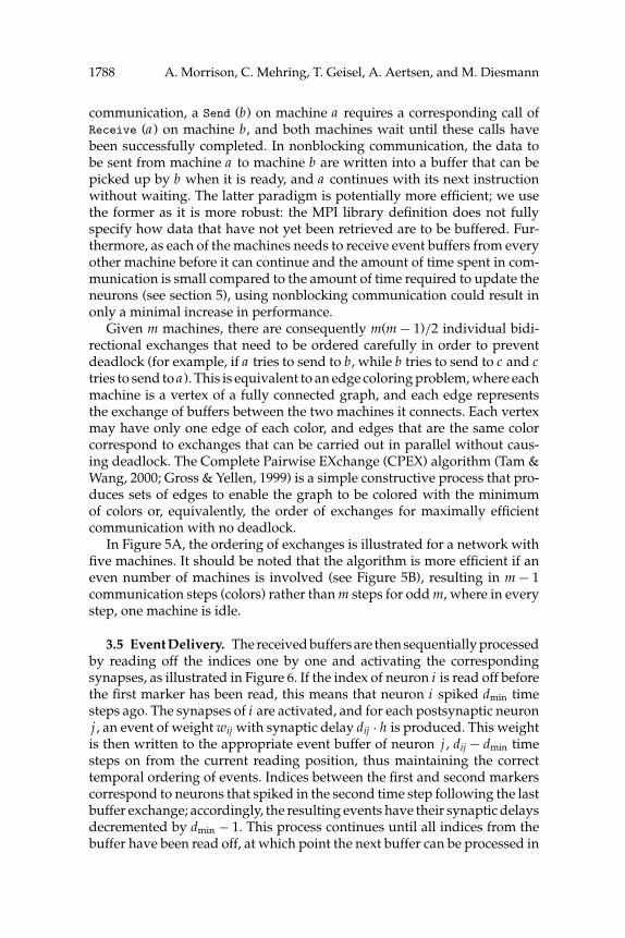
1788 A. Morrison, C. Mehring, T. Geisel, A. Aertsen, and M. Diesmann
communication, a Send (b) on machine a requires a corresponding call ofReceive (a ) on machine b, and both machines wait until these calls havebeen successfully completed. In nonblocking communication, the data tobe sent from machine a to machine b are written into a buffer that can bepicked up by b when it is ready, and a continues with its next instructionwithout waiting. The latter paradigm is potentially more efficient; we usethe former as it is more robust: the MPI library definition does not fullyspecify how data that have not yet been retrieved are to be buffered. Fur-thermore, as each of the machines needs to receive event buffers from everyother machine before it can continue and the amount of time spent in com-munication is small compared to the amount of time required to update theneurons (see section 5), using nonblocking communication could result inonly a minimal increase in performance.
Given m machines, there are consequently m(m − 1)/2 individual bidi-rectional exchanges that need to be ordered carefully in order to preventdeadlock (for example, if a tries to send to b, while b tries to send to c and ctries to send to a ). This is equivalent to an edge coloring problem, where eachmachine is a vertex of a fully connected graph, and each edge representsthe exchange of buffers between the two machines it connects. Each vertexmay have only one edge of each color, and edges that are the same colorcorrespond to exchanges that can be carried out in parallel without caus-ing deadlock. The Complete Pairwise EXchange (CPEX) algorithm (Tam &Wang, 2000; Gross & Yellen, 1999) is a simple constructive process that pro-duces sets of edges to enable the graph to be colored with the minimumof colors or, equivalently, the order of exchanges for maximally efficientcommunication with no deadlock.
In Figure 5A, the ordering of exchanges is illustrated for a network withfive machines. It should be noted that the algorithm is more efficient if aneven number of machines is involved (see Figure 5B), resulting in m − 1communication steps (colors) rather than m steps for odd m, where in everystep, one machine is idle.
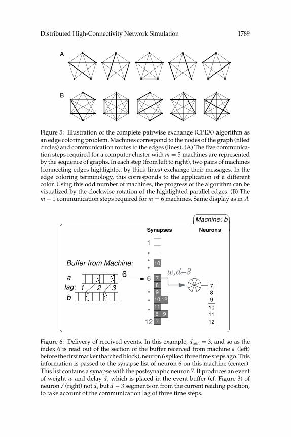
3.5 Event Delivery. The received buffers are then sequentially processedby reading off the indices one by one and activating the correspondingsynapses, as illustrated in Figure 6. If the index of neuron i is read off beforethe first marker has been read, this means that neuron i spiked dmin timesteps ago. The synapses of i are activated, and for each postsynaptic neuronj , an event of weight wij with synaptic delay dij · h is produced. This weightis then written to the appropriate event buffer of neuron j , dij − dmin timesteps on from the current reading position, thus maintaining the correcttemporal ordering of events. Indices between the first and second markerscorrespond to neurons that spiked in the second time step following the lastbuffer exchange; accordingly, the resulting events have their synaptic delaysdecremented by dmin − 1. This process continues until all indices from thebuffer have been read off, at which point the next buffer can be processed in
Distributed High-Connectivity Network Simulation 1789
A
B
Figure 5: Illustration of the complete pairwise exchange (CPEX) algorithm asan edge coloring problem. Machines correspond to the nodes of the graph (filledcircles) and communication routes to the edges (lines). (A) The five communica-tion steps required for a computer cluster with m = 5 machines are representedby the sequence of graphs. In each step (from left to right), two pairs of machines(connecting edges highlighted by thick lines) exchange their messages. In theedge coloring terminology, this corresponds to the application of a differentcolor. Using this odd number of machines, the progress of the algorithm can bevisualized by the clockwise rotation of the highlighted parallel edges. (B) Them − 1 communication steps required for m = 6 machines. Same display as in A.
1210
98
10
789
11
7
10
1211
98
blag: 1 2 3a
Buffer from Machine:
NeuronsSynapses
6
1
12
6w,d–3
7
Machine: b
Figure 6: Delivery of received events. In this example, dmin = 3, and so as theindex 6 is read out of the section of the buffer received from machine a (left)before the first marker (hatched block), neuron 6 spiked three time steps ago. Thisinformation is passed to the synapse list of neuron 6 on this machine (center).This list contains a synapse with the postsynaptic neuron 7. It produces an eventof weight w and delay d, which is placed in the event buffer (cf. Figure 3) ofneuron 7 (right) not d , but d − 3 segments on from the current reading position,to take account of the communication lag of three time steps.
1790 A. Morrison, C. Mehring, T. Geisel, A. Aertsen, and M. Diesmann
the same way. Once all buffers have been processed, the next dmin · h periodin the life of the network is simulated, and the cycle begins again.
4 Random Numbers
Many networks require a massive amount of random numbers for their sim-ulation and construction. In addition to the usual pitfalls of pseudorandomnumber generation, this presents extra problems in a distributed environ-ment. The ideal solution should be able to produce sequences of randomnumbers for each machine such that each sequence is itself uncorrelated,and each sequence is uncorrelated to any other sequence. Furthermore,it should be possible to perform a simulation on a different hardware orwith a different number of machines, and obtain identical results. A centralrandom number server is not an appropriate solution for this application,as this would result in a bottleneck due to the sheer volume of numbersrequired. A partial solution is provided by the use of random number gen-erators (RNGs), which produce independent trajectories for different seeds(Knuth, 1997). Such RNGs are available from the GNU Scientific Library(Galassi, Gough, & Jungman, 2001), which, moreover, ensures platform in-dependence.
The solution is completed by the introduction of pseudoprocesses. Thenumber of pseudoprocesses Npp is specified at run time, when the numberof machines used m is also known. They are assigned to the machines suchthat pseudoprocess p is on machine p mod m, and each machine has an equalnumber of pseudoprocesses, thereby constraining m to be a factor of Npp.Each pseudoprocess is assigned one RNG with a unique seed. Each neuron isassigned to a pseudoprocess such that neuron n is assigned to pseudoprocessn mod Npp, and all the random numbers required for that neuron are drawnfrom the corresponding RNG. As the algorithm to assign the neurons to thepseudoprocesses depends solely on Npp, identical simulation results will beobtained for any m fulfilling the constraint. In this way, we ensure a fast,safe production of random numbers, independent of both the platform andthe number of machines used.
5 Performance
We tested the software on four architectures, chosen to reflect the kind ofhardware currently available:
� Elderly PC cluster (8 × 2 processors, 100 MBit Ethernet, Intel Pentium0.8 GHz, 256 kB cache)
� Recent PC cluster (20 × 2 processors, Dolphin/Scali network, IntelXeon, 2.8 GHz, 512 kB cache)
� Compaq GS160 (16 processors, Alpha 0.7 GHz, 8 MB cache)
Distributed High-Connectivity Network Simulation 1791
1 2 4 8 16
1
2
4
8
16
32
time
[s]
machines1 2 4 8 16
100
200
400
800
1600
3200
6400
time
[s]
machines
A B
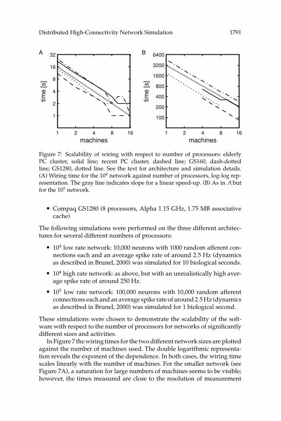
Figure 7: Scalability of wiring with respect to number of processors: elderlyPC cluster, solid line; recent PC cluster, dashed line; GS160, dash-dottedline; GS1280, dotted line. See the text for architecture and simulation details.(A) Wiring time for the 104 network against number of processors, log-log rep-resentation. The gray line indicates slope for a linear speed-up. (B) As in A butfor the 105 network.
� Compaq GS1280 (8 processors, Alpha 1.15 GHz, 1.75 MB associativecache)
The following simulations were performed on the three different architec-tures for several different numbers of processors:
� 104 low rate network: 10,000 neurons with 1000 random afferent con-nections each and an average spike rate of around 2.5 Hz (dynamicsas described in Brunel, 2000) was simulated for 10 biological seconds.
� 104 high rate network: as above, but with an unrealistically high aver-age spike rate of around 250 Hz.
� 105 low rate network: 100,000 neurons with 10,000 random afferentconnections each and an average spike rate of around 2.5 Hz (dynamicsas described in Brunel, 2000) was simulated for 1 biological second.
These simulations were chosen to demonstrate the scalability of the soft-ware with respect to the number of processors for networks of significantlydifferent sizes and activities.
In Figure 7 the wiring times for the two different network sizes are plottedagainst the number of machines used. The double logarithmic representa-tion reveals the exponent of the dependence. In both cases, the wiring timescales linearly with the number of machines. For the smaller network (seeFigure 7A), a saturation for large numbers of machines seems to be visible;however, the times measured are close to the resolution of measurement
1792 A. Morrison, C. Mehring, T. Geisel, A. Aertsen, and M. Diesmann
1 2 4 8 16
100
200
400
800
1600
3200
6400tim
e [
s]
machines1 4 8 12 16
0
0.2
0.4
0.6
0.8
1
machines
spe
ed
-up
fa
cto
r
(A) (B)
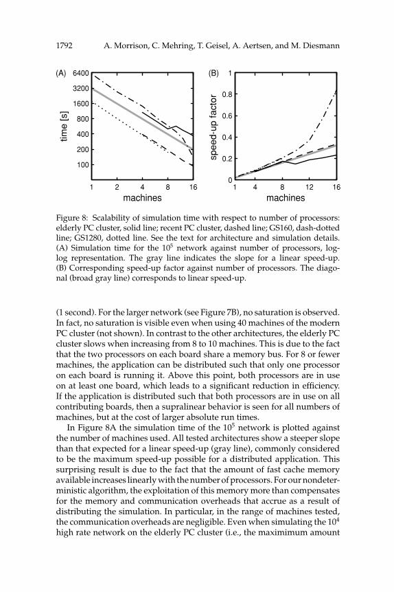
Figure 8: Scalability of simulation time with respect to number of processors:elderly PC cluster, solid line; recent PC cluster, dashed line; GS160, dash-dottedline; GS1280, dotted line. See the text for architecture and simulation details.(A) Simulation time for the 105 network against number of processors, log-log representation. The gray line indicates the slope for a linear speed-up.(B) Corresponding speed-up factor against number of processors. The diago-nal (broad gray line) corresponds to linear speed-up.
(1 second). For the larger network (see Figure 7B), no saturation is observed.In fact, no saturation is visible even when using 40 machines of the modernPC cluster (not shown). In contrast to the other architectures, the elderly PCcluster slows when increasing from 8 to 10 machines. This is due to the factthat the two processors on each board share a memory bus. For 8 or fewermachines, the application can be distributed such that only one processoron each board is running it. Above this point, both processors are in useon at least one board, which leads to a significant reduction in efficiency.If the application is distributed such that both processors are in use on allcontributing boards, then a supralinear behavior is seen for all numbers ofmachines, but at the cost of larger absolute run times.
In Figure 8A the simulation time of the 105 network is plotted againstthe number of machines used. All tested architectures show a steeper slopethan that expected for a linear speed-up (gray line), commonly consideredto be the maximum speed-up possible for a distributed application. Thissurprising result is due to the fact that the amount of fast cache memoryavailable increases linearly with the number of processors. For our nondeter-ministic algorithm, the exploitation of this memory more than compensatesfor the memory and communication overheads that accrue as a result ofdistributing the simulation. In particular, in the range of machines tested,the communication overheads are negligible. Even when simulating the 104
high rate network on the elderly PC cluster (i.e., the maximimum amount
Distributed High-Connectivity Network Simulation 1793
0
200
400
600
800
1000
1200
low rate 104 high rate 104 low rate 105
time
[s]
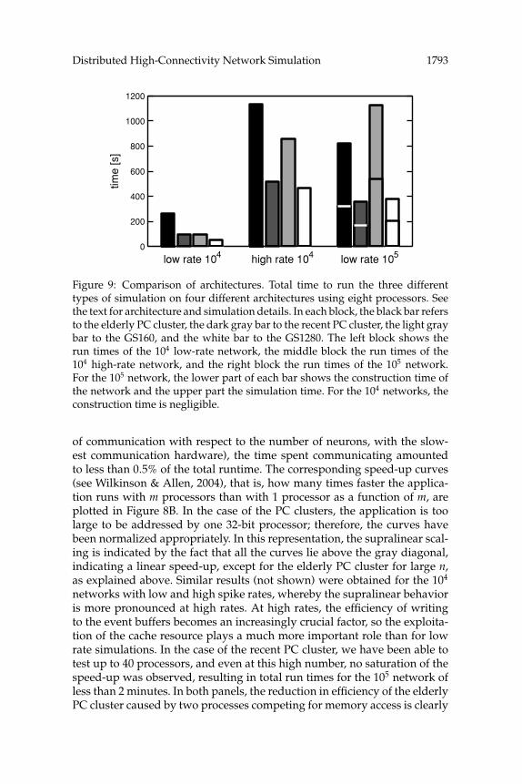
Figure 9: Comparison of architectures. Total time to run the three differenttypes of simulation on four different architectures using eight processors. Seethe text for architecture and simulation details. In each block, the black bar refersto the elderly PC cluster, the dark gray bar to the recent PC cluster, the light graybar to the GS160, and the white bar to the GS1280. The left block shows therun times of the 104 low-rate network, the middle block the run times of the104 high-rate network, and the right block the run times of the 105 network.For the 105 network, the lower part of each bar shows the construction time ofthe network and the upper part the simulation time. For the 104 networks, theconstruction time is negligible.
of communication with respect to the number of neurons, with the slow-est communication hardware), the time spent communicating amountedto less than 0.5% of the total runtime. The corresponding speed-up curves(see Wilkinson & Allen, 2004), that is, how many times faster the applica-tion runs with m processors than with 1 processor as a function of m, areplotted in Figure 8B. In the case of the PC clusters, the application is toolarge to be addressed by one 32-bit processor; therefore, the curves havebeen normalized appropriately. In this representation, the supralinear scal-ing is indicated by the fact that all the curves lie above the gray diagonal,indicating a linear speed-up, except for the elderly PC cluster for large n,as explained above. Similar results (not shown) were obtained for the 104
networks with low and high spike rates, whereby the supralinear behavioris more pronounced at high rates. At high rates, the efficiency of writingto the event buffers becomes an increasingly crucial factor, so the exploita-tion of the cache resource plays a much more important role than for lowrate simulations. In the case of the recent PC cluster, we have been able totest up to 40 processors, and even at this high number, no saturation of thespeed-up was observed, resulting in total run times for the 105 network ofless than 2 minutes. In both panels, the reduction in efficiency of the elderlyPC cluster caused by two processes competing for memory access is clearly
1794 A. Morrison, C. Mehring, T. Geisel, A. Aertsen, and M. Diesmann
0 25 50 75 1000
0.2
0.4
0.6
0.8
1
rate [Hz]
time
[s]
1 2 4 8 16 32 64
10
20
50
100
200
400
800
1600
3200
time
[s]
neurons [× 10 ]4
A B
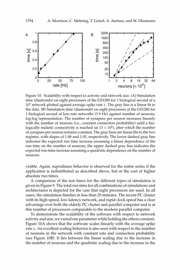
Figure 10: Scalability with respect to activity and network size. (A) Simulationtime (diamonds) on eight processors of the GS1280 for 1 biological second of a104 network plotted against average spike rate λ. The gray line is a linear fit tothe data. (B) Simulation time (diamonds) on eight processors of the GS1280 for1 biological second of low-rate networks (3.9 Hz) against number of neurons,log-log representation. The number of synapses per neuron increases linearlywith the number of neurons (i.e., constant connection probability) until a bio-logically realistic connectivity is reached (at 13 × 104), after which the numberof synapses per neuron remains constant. The gray lines are linear fits to the tworegimes, with slopes of 1.88 and 1.05, respectively. The lower dashed gray lineindicates the expected run time increase assuming a linear dependence of therun time on the number of neurons; the upper dashed gray line indicates theexpected run-time increase assuming a quadratic dependence on the number ofneurons.
visible. Again, supralinear behavior is observed for the entire series if theapplication is redistributed as described above, but at the cost of higherabsolute run times.
A comparison of the run times for the different types of simulation isgiven in Figure 9. The total run time for all combinations of simulations andarchitectures is depicted for the case that eight processors are used. In allcases, the simulation finishes in less than 20 minutes. The recent PC clusterwith its high-speed, low-latency network, and rapid clock speed has a clearadvantage over both the elderly PC cluster and parallel computer and is atthis number of processors comparable to the modern parallel computer.
To demonstrate the scalability of the software with respect to networkactivity and size, we varied one parameter while holding the others constant.Figure 10A shows that the software scales linearly with the average spikerate λ. An excellent scaling behavior is also seen with respect to the numberof neurons in the network with constant rate and connection probability(see Figure 10B). It lies between the linear scaling due to the increase inthe number of neurons and the quadratic scaling due to the increase in the
Distributed High-Connectivity Network Simulation 1795
1 2 3 4 5 6 7 8 90.9
0.95
1
1.05
1.1re
lativ
e tim
e
neurons [× 10 ]5
1 2 4 6 8
machines
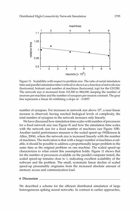
Figure 11: Scalability with respect to problem size. The ratio of serial simulationtime and parallel simulation time (vertical) is shown as a function of network size(horizontal, bottom) and number of machines (horizontal, top) for the GS1280.The network size is increased from 110,500 to 884,000, keeping the number ofneurons per machine and the number of synapses per neuron constant. The grayline represents a linear fit exhibiting a slope of −0.0057.
number of synapses. For increases in network size above 105, a near-linearincrease is observed; having reached biological levels of complexity, thetotal number of synapses in the network increases only linearly.
We have discussed how simulation time scales with number of processorsfor a fixed network size (see Figure 8) and how the simulation time scaleswith the network size for a fixed number of machines (see Figure 10B).Another useful performance measure is the scaled speed-up (Wilkinson &Allen, 2004), where the network size is increased linearly with the numberof machines. The motivation is that with a larger number of machines avail-able, it should be possible to address a proportionally larger problem in thesame time as the original problem on one machine. The scaled speed-upcharacterizes to what extent this assumption holds. Figure 11 shows thatfor the number of processors available on the parallel computer tested, thescaled speed-up remains close to 1, indicating excellent scalability of thesoftware and the problem. The small, systematic linear decline of scaledspeed-up presumably originates from the increased absolute amount ofmemory access and communication load.
6 Discussion
We described a scheme for the efficient distributed simulation of largeheterogeneous spiking neural networks. In contrast to earlier approaches,
1796 A. Morrison, C. Mehring, T. Geisel, A. Aertsen, and M. Diesmann
the simulation technology enables the investigation of recurrent networkswith levels of connectivity and sparseness characteristic for the mammalianbrain. A network of 100,000 neurons permits a biologically realistic numberof synapses per neuron (of the order of 104) while simultaneously adheringto a biologically realistic constraint on the connection probability betweentwo neurons (of the order of 0.1 in the local volume). In this sense, sucha network constitutes a threshold size for realistic simulations of corticalnetworks. The technology described in this article easily overcomes thisthreshold on available hardware, requiring wall clock times suitable forroutine use. For larger neural systems, the required computer memory andwall clock time scale merely linearly (as opposed to quadratically) with thenumber of neurons.
The neural network to be simulated can be distributed over many com-puters. Execution time and the computer memory required on an individualmachine scale excellently with the number of machines used. As a conse-quence of the considerations above, larger networks can be simulated, ora reduction in execution time achieved, simply by adding a proportionatenumber of computers to the system. In addition to the distributed simula-tion of the dynamics, an important feature of our technology is the parallelgeneration of the network structure. A serial construction of the networkwould severely limit the speed-up, as the time required to construct thenetwork can constitute a considerable fraction of the total execution time(see Figure 9). A similar argument holds for the generation of random num-bers, which can also easily become the component limiting the speed-up.Consequently, the generation of random number is parallelized, and careis taken that simulation results are independent of the number of machinesused to carry out the simulation.
The efficiency of the simulation scheme results from exploiting the factthat the interaction of network elements is noninstantaneous and mediatedby point events (spikes). The frequency and bulk of the communicationbetween machines are independent of the computation step size (precisionof the simulation). The simulation scheme profits from the fact that thefast cache memory increases proportionally with the number of machines,reducing the ratio between the locally required working memory and thelocally available cache (Wilkinson & Allen, 2004). Surprisingly, the increasein simulation speed gained more than compensates the overhead due to thecommunication in a distributed environment. Overall, a supralinear speed-up is observed, justifying the use of large clusters of computers. A detailedquantitative investigation of cache effects is outside the scope of this study.However, it is evident from the results presented that when deciding onhardware for a simulation project using our scheme, not only the clockspeed of the processors but also the amount of cache memory should beconsidered.
We pointed out in section 3.1 that neither of the textbook simulationschemes, discrete time and event-driven algorithms, is optimal for the
Distributed High-Connectivity Network Simulation 1797
simulation of biological neural networks. Instead, only a carefully adjustedhybrid of both leads to a satisfactory run-time behavior. A similar obser-vation is made with respect to the class design of the software compo-nents (cf. the comment on this observation in Gamma, Helm, Johnson, &Vlissides, 1994). Only a well-balanced mixture of objects from the problemdomain (neurobiology) and from the machine-oriented domain of paral-lel algorithms leads to a design that appropriately compromises betweenthe heterogeneity of biological structure, usability of the software, and theefficiency of the simulation on today’s computer hardware. Both obser-vations argue for a pragmatic and undogmatic usage of software designprinciples and the selection of an implementation language supportingmultiple paradigms (Stroustrup, 1994). Ideally, the interface with whichthe researcher, attempting to implement a new neuron model, is confrontedwould be expressed in terms of neuroscience concepts and objects, while theobjects of the software layer below are optimized for cache exploitation andefficient communication. We have made some first steps in this direction, butfurther research is required to work out how this approach can consistentlybe applied to the different components of the simulation scheme.
Future work on this topic falls broadly into two categories: optimizationand functionality. With respect to the former, the clearly observable cache ef-fects suggest that much could be gained by optimizing the data structures ac-cordingly. We are currently testing various alternative representations of thenetwork structure and update schemes in order to enhance the cache usage,particularly for low numbers of machines. Furthermore, the load balancingcurrently carried out by the simulation kernel is minimal and relies on thestatic uniform distribution of network elements and their types over theavailable machines. Thus, efficient use of the hardware resources requireshomogeneous computer clusters. While in the context of high-performancecomputing this does not represent a major constraint, the limitation be-comes relevant when more structured networks are investigated with largedifferences in the communication load between and within subnetworks.The next step in addressing the problem of load balancing would be to pro-vide user-level control over the mapping of network elements to machines.Finally, the results presented in this article demonstrate that it is possibleand efficient to execute our code on computers with multiple processors.However, the use of a communication protocol developed under the con-straints of distributed computing (Pacheco, 1997) does not fully exploit theexistence of a working memory addressable by all processors. In the frame-work of the NEST initiative (www.nest-initiative.org) we are developingthe simulation technology for computers with multiple processors. Currenttrends in computer hardware toward clusters of multiprocessor machines,whereby each machine has a small number of processors and support formultithreading (Butenhof, 1997) in the individual processors, makes a hy-brid simulation kernel using multithreading locally and message passingbetween computers increasingly interesting.
1798 A. Morrison, C. Mehring, T. Geisel, A. Aertsen, and M. Diesmann
One factor limiting the usability of the software described here is thatthe protocol for a particular simulation experiment must be specified by aC++ program. In a parallel line of work, we are developing a simulationlanguage interpreter enabling the interactive specification and manipula-tion of neural systems simulations (Diesmann & Gewaltig, 2002). It remainsto be investigated how the distributed simulation kernel can be combinedwith this interpreter. Other current work (Morrison, Hake, Straube, Plesser,& Diesmann, 2005) focuses on extending the functional range of the technol-ogy through the incorporation of precise (off-grid) spike times (see Hansel,Mato, Meunier, & Neltner, 1998; Rotter & Diesmann, 1999; Shelley & Tao,2001, for discussion) and spike-time-dependent plasticity (Morrison, Aert-sen, & Diesmann, 2004) into the simulation scheme. In future projects, struc-tural plasticity and the interaction of spiking neural networks with modu-latory chemical subsystems will also be addressed.
Acknowledgments
We acknowledge constructive discussions with Denny Fliegner, StefanRotter, Masayoshi Kubo, and the members of the NEST collaboration (inparticular Marc-Oliver Gewaltig and Hans Ekkehard Plesser). This workwas partially funded by the Volkswagen Foundation, GIF, BIF, DIP F1.2,DAAD 313-PPP-N4-lk, and BMBF Grant 01GQ0420 to BCCN Freiburg. Allsimulations have been carried out using the parallel computing facilities ofthe Max-Planck-Institute for Fluid Dynamics (now MPI for Dynamics andSelf Organization) in Gottingen and the Agricultural University of Norwayin As. Part of the work was carried out when A. M. and M. D. were basedat the Max-Planck-Institute for Fluid Dynamics. The initial distributed ver-sion of the simulation software was developed by Mehring in the contextof Mehring, et al. (2003).
References
Abbott, L. F., & Nelson, S. B. (2000). Synaptic plasticity: Taming the beast. Nat. Neu-rosci., 3(Suppl.), 1178–1183.
Abeles, M. (1982). Local cortical circuits: An electrophysiological study. Berlin: Springer-Verlag.
Abeles, M. (1991). Corticonics: Neural circuits of the cerebral cortex. Cambridge: Cam-bridge University Press.
Aertsen, A., Gerstein, G., Habib, M., & Palm, G. (1989). Dynamics of neuronal firingcorrelation: Modulation of “effective connectivity.” J. Neurophysiol., 61(5), 900–917.
Aho, A. V., Hopcroft, J. E., & Ullman, J. D. (1983). Data structures and algorithms.Reading, MA: Addison-Wesley.
Aviel, Y., Mehring, C., Abeles, M., & Horn, D. (2003). On embedding synfire chainsin a balanced network. Neural Comput., 15(6), 1321–1340.
Distributed High-Connectivity Network Simulation 1799
Bernard, C., Ge, Y. C., Stockley, E., Willis, J. B., & Wheal, H. V. (1994). Synap-tic integration of NMDA and non-NMDA receptors in large neuronal net-work models solved by means of differential equations. Biol. Cybern., 70, 267–273.
Bi, G.-q., & Poo, M.-m. (1998). Activity-induced synaptic modifications in hippocam-pal culture: Dependence on spike timing, synaptic strength and cell type. J. Neu-rosci., 18, 10464–10472.
Bi, G., & Poo, M. (2001). Synaptic modification by correlated activity: Hebb’s postulaterevisited. Annu. Rev. of Neurosci., 24, 139–166.
Bower, J. M., & Beeman, D. (1997). The book of GENESIS: Exploring realistic neuralmodels with the GEneral NEural SImulation System (2nd ed.). New York: TELOS,Springer-Verlag.
Braitenberg, V. (1978). Cell assemblies in the cerebral cortex. In R. Heim & G. Palm(Eds.), Theoretical approaches to complex systems. Berlin: Springer.
Braitenberg, V., & Schuz, A. (1998). Cortex: Statistics and geometry of neuronal connec-tivity (2nd ed.). Berlin: Springer-Verlag.
Brunel, N. (2000). Dynamics of sparsely connected networks of excitatory and in-hibitory spiking neurons. J. Comput. Neurosci., 8(3), 183–208.
Butenhof, D. R. (1997). Programming with POSIX threads. Reading, MA: Addison-Wesley.
Chance, F. S., Abbott, L. F., & Reyes, A. D. (2002). Gain modulation from backgroundsynaptic input. Neuron, 35, 773–782.
Dayan, P., & Abbott, L. F. (2001). Theoretical neuroscience. Cambridge, MA: MIT Press.Delorme, A., & Thorpe, S. (2003). Spikenet: An event-driven simulation package for
modeling large networks of spiking neurons. Network: Comput. Neural Systems, 14,613–627.
Destexhe, A., Rudolph, M., & Pare, D. (2003). The high-conductance state of neocor-tical neurons in vivo. Nat. Rev. Neurosci., 4, 739–751.
Diesmann, M., & Gewaltig, M.-O. (2002). NEST: An environment for neural systemssimulations. In T. Plesser & V. Macho (Eds.), Forschung und wisschenschaftlichesRechnen, Beitrage zum Heinz-Billing-Preis 2001 (pp. 43–70). Gottingen: Ges. furWiss. Datenverarbeitung.
Diesmann, M., Gewaltig, M.-O., & Aertsen, A. (1995). SYNOD: An environment forneural systems simulations: Language interface and tutorial (Tech. Rep. GC-AA-/95-3). Tel Aviv: Weizmann Institute of Science.
Diesmann, M., Gewaltig, M.-O., & Aertsen, A. (1999). Stable propagation of syn-chronous spiking in cortical neural networks. Nature, 402, 529–533.
Diesmann, M., Gewaltig, M.-O., Rotter, S., & Aertsen, A. (2001). State space analysisof synchronous spiking in cortical neural networks. Neurocomputing, 38–40, 565–571.
Ermentrout, B. (2002). Simulating, analyzing, and animating dynamical systems: A guideto Xppaut for researchers and students (software, environments, tools). Philadelphia:Society for Industrial and Applied Math.
Galassi, M., Gough, B., & Jungman, G. (2001). Gnu scientific library: Reference manual.Bristol, UK: Network Theory Ltd.
Gamma, E., Helm, R., Johnson, R., & Vlissides, J. (1994). Design patterns: Elements ofreusable object-oriented Software. Reading, MA: Addison-Wesely.
1800 A. Morrison, C. Mehring, T. Geisel, A. Aertsen, and M. Diesmann
Gerstein, G. L., Bedenbaugh, P., & Aertsen, A. (1989). Neuronal assemblies. IEEETrans. Biomed. Eng., 36, 4–14.
Gewaltig, M.-O. (2000). Evolution of synchronous spike volleys in cortical Networks: Net-work simulations and continuous probabilistic models. Aachen, Germany: Shaker.
Gross, J., & Yellen, J. (1999). Graph theory and its applications. Boca Ratan, FL: CRCPress.
Hansel, D., Mato, G., Meunier, C., & Neltner, L. (1998). On numerical simulations ofintegrate-and-fire neural networks. Neural Comput., 10(2), 467–483.
Hawkes, A. G. (1971). Point spectra of some mutually exciting point processes. Journalof the Royal Statistical Society (London) B, 33, 438–443.
Hebb, D. O. (1949). Organization of behavior: A neurophysiological theory. New York:Wiley.
Hines, M., & Carnevale, N. T. (1997). The NEURON simulation environment. NeuralComput., 9, 1179–1209.
Jack, J. J. B., Noble, D., & Tsien, R. W. (1983). Electric current flow in excitable cells. NewYork: Oxford University Press.
Knuth, D. E. (1997). The art of computer programming: Seminumerical algorithms(3rd ed., Vol. 2). Reading, MA: Addison-Wesley.
Koch, C. (1999). Biophysics of computation: Information processing in single neurons. NewYork: Oxford University Press.
Koch, C., & Segev, I. (1989). Methods in neuronal modeling. Cambridge, MA: MIT Press.Kuhn, A., Aertsen, A., & Rotter, S. (2003). Higher-order statistics of input ensembles
and the response of simple model neurons. Neural Comput., 15(1), 67–101.Kuhn, A., Aertsen, A., & Rotter, S. (2004). Neuronal integration of synaptic input in
the fluctuation-driven regime. J. Neurosci., 24, 2345–2356.Kumar, A., Kremkow, J., Rotter, S., & Aertsen, A. (2004). Synaptic integration in a
3-compartment model of layer 5 pyramidal neurons. FENS Abstr., 2, A014.27.Larkum, M., Zhu, J., & Sakmann, B. (2001). Dendritic mechanisms underlying the
coupling of the dendritic with the axonal action potential initiation zone of adultrat layer 5 pyramidal neurons. J. Neurophysiol., 533 (pt. 2), 447–466.
Lee, G., & Farhat, N. H. (2001). The double queue method: A numerical method forintegrate-and-fire neuron networks. Neural Networks, 14, 921–932.
Markram, H., & Tsodyks, M. (1996). Redistribution of synaptic efficacy betweenneocortical pyramidal neurons. Nature, 382(6594), 807–810.
Mattia, M., & Del Giudice, P. (2000). Efficient event-driven simulation of large net-works of spiking neurons and dynamical synapses. Neural Comput., 12(10), 2305–2329.
Mehring, C., Hehl, U., Kubo, M., Diesmann, M., & Aertsen, A. (2003). Activity dy-namics and propagation of synchronous spiking in locally connected randomnetworks. Biol. Cybern. 88(5), 395–408.
Morrison, A., Aertsen, A., & Diesmann, M. (2004). Stability of plastic recurrent networks.Paper presented at the Monte Verita Workshop on Spike-Timing Dependent Plas-ticity, Monte Verita, Ascona, Switzerland.
Morrison, A., Hake, J., Straube, S., Plesser, H. E., & Diesmann, M. (2005). Precisespike timing with exact subthreshold integration in discrete time network simu-lations. In Proceedings of the 30th Gottingen Neurobiology Conference, NeuroforumSupplement 1, pp. 205B.
Distributed High-Connectivity Network Simulation 1801
Morrison, A., Mehring, C., Diesmann, M., Aertsen, A., & Geisel, T. (2003). Distributedsimulation of large biological neural networks. In Proceedings of the 29th GottingenNeurobiology Conference, (p. 590).
Pacheco, P. S. (1997). Parallel programming with MPI. San Francisco: Morgan Kauf-mann.
Palm, G. (1990). Cell assemblies as a guideline for brain research. Conc. Neurosci., 1,133–148.
Reutimann, J., Giugliano, M., & Fusi, S. (2003). Event-driven simulation of spikingneurons with stochastic dynamics. Neural Comput., 15, 811–830.
Rotter, S., & Diesmann, M. (1999). Exact digital simulation of time-invariant linearsystems with applications to neuronal modeling. Biol. Cybern., 81(5/6), 381–402.
Salinas, E., & Sejnowski, T. J. (2000). Impact of correlated synaptic input on outputfiring rate and variability in simple neuronal models. J. Neurosci., 20(16), 6193–6209.
Shadlen, M. N., & Newsome, W. T. (1998). The variable discharge of cortical neu-rons: Implications for connectivity, computation, and information coding. J. Neu-rosci., 18(10), 3870–3896.
Shelley, M. J., & Tao, L. (2001). Efficient and accurate time-stepping schemes forintegrate-and-fire neuronal networks. J. Comput. Neurosci., 11(2), 111–119.
Singer, W. (1993). Synchronization of cortical activity and its putative role in infor-mation processing and learning. Annu. Rev. Physiol., 55, 349–374.
Singer, W. (1999). Time as coding space. Curr. Opin. Neurobiol., 9(2), 189–194.Stroustrup, B. (1994). The design and evolution of C++. Reading, MA: Addison-Wesley.Stroustrup, B. (1997). The C++ programming language (3 ed.). Reading, MA: Addison-
Wesley.Tam, A., & Wang, C. (2000). Efficient scheduling of complete exchange on clusters. In
G. Chaudhry & E. Sha (Eds.), 13th International Conference on Parallel and DistributedComputing Systems (PDCS 2000). Cary, NC: International Society for Computersand Their Applications.
Tetzlaff, T., Morrison, A., Geisel, T., & Diesmann, M. (2004). Consequences of realisticnetwork size on the stability of embedded synfire chains. Neurocomputing, 58–60,117–121.
Thomson, A. M., & Deuchars, J. (1994). Temporal and spatial properties of localcircuits in neocortex. TINS, 17, 119–126.
von der Malsburg, C. (1981). The correlation theory of brain function (Internal Rep. 81-2).Gottingen: Max-Planck-Institute for Biophysical Chemistry.
von der Malsburg, C. (1986). Am I thinking assemblies? In G. Palm & A. Aertsen(Eds.), Brain theory (pp. 161–176) Berlin: Springer-Verlag.
Wilkinson, B., & Allen, M. (2004). Parallel programming: Techniques and applicationsusing networked workstations and parallel computers (2nd ed.). Upper Saddle River,NJ: Prentice Hall.
Received July 20, 2004; accepted January 31, 2005.