PDE and Boundary-Value Problems Winter Term 2016/2017 PDE and Boundary-Value Problems Winter Term...
29
PDE and Boundary-Value Problems Winter Term 2016/2017 Lecture 4 Saarland University 11 November 2016 c Daria Apushkinskaya (UdS) PDE and BVP lecture 4 11 November 2016 1 / 29
Transcript of PDE and Boundary-Value Problems Winter Term 2016/2017 PDE and Boundary-Value Problems Winter Term...

PDE and Boundary-Value ProblemsWinter Term 2016/2017
Lecture 4
Saarland University
11 November 2016
c© Daria Apushkinskaya (UdS) PDE and BVP lecture 4 11 November 2016 1 / 29

Purpose of Lesson
To discuss the second and the third important types of BCs:
temperature of the surrounded medium specified,
heat flow across the boundary specified.
To show how the one-space dimensional heat equation
ut = α2uxx + f (x , t)
is derived from the basic principle of conservation of heat .
To show how the rate of heat transfer depends on thermalconductivity , thermal capacity , and density .
To discuss a few variations of the basic heat equation.
c© Daria Apushkinskaya (UdS) PDE and BVP lecture 4 11 November 2016 2 / 29

Boundary conditions for parabolic-type problems Type 2 BC
Type 2 BC (Temperature of the surrounding mediumspecified)
Suppose we have the following experiment that we again break intosteps:
1. We consider again our laterally insulated copper rod. Recall thatlaterally insulated means: heat can flow in and out of the rod atthe ends, but not across the lateral boundary.
2. We put the left side of the rod in a container that has a changingtemperature g1(t), while the right end is putted in another liquidwith temperature g2(t).
c© Daria Apushkinskaya (UdS) PDE and BVP lecture 4 11 November 2016 3 / 29

Boundary conditions for parabolic-type problems Type 2 BC
Type 2 BC (Temperature of the surrounding mediumspecified)
1 We cannot say the boundary temperatures of the rod will be thesame as the liquid temperatures g1(t) and g2(t).
2 We know (Newton’s law of cooling) that whenever the rodtemperature at one of the boundaries is less than the respectiveliquid temperatures, then heat will flow into the rod at a rateproportional to this difference.
c© Daria Apushkinskaya (UdS) PDE and BVP lecture 4 11 November 2016 4 / 29
Boundary conditions for parabolic-type problems Type 2 BC
Type 2 BC (Temperature of the surrounding mediumspecified)
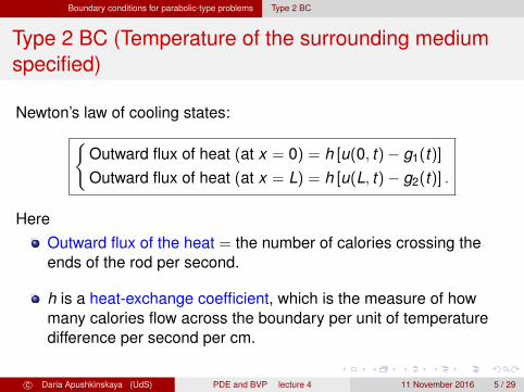
Newton’s law of cooling states:{Outward flux of heat (at x = 0) = h [u(0, t)− g1(t)]
Outward flux of heat (at x = L) = h [u(L, t)− g2(t)] .
HereOutward flux of the heat = the number of calories crossing theends of the rod per second.
h is a heat-exchange coefficient, which is the measure of howmany calories flow across the boundary per unit of temperaturedifference per second per cm.
c© Daria Apushkinskaya (UdS) PDE and BVP lecture 4 11 November 2016 5 / 29
Boundary conditions for parabolic-type problems Type 2 BC
Type 2 BC (Temperature of the surrounding mediumspecified)
RemarkNote that the outward flux of heat will be positive at either end providedthe temperature of the rod is greater than the surrounding medium.
Otherwise, the outward flux of heat will be negative at either endprovided the temperature of the rod is less than the surroundingmedium.
c© Daria Apushkinskaya (UdS) PDE and BVP lecture 4 11 November 2016 6 / 29

Boundary conditions for parabolic-type problems Type 2 BC
Type 2 BC (Temperature of the surrounding mediumspecified)
In addition to Newton’s law we state Fourier’s law (provenexperimentally)
Outward flux of heat across a boundary is proportionalto the inward normal derivative across the boundary
This law says that if the temperature is increasing rapidly in thedirection outward from the boundary of a domain, then heat will flowfrom the surrounding medium into the domain.
c© Daria Apushkinskaya (UdS) PDE and BVP lecture 4 11 November 2016 7 / 29

Boundary conditions for parabolic-type problems Type 2 BC
Type 2 BC (Temperature of the surrounding mediumspecified)
In our 1-dimensional problem, Fourier’s law takes the form:
Outward flux of heat (at x = 0) = k
∂u(0, t)∂x
Outward flux of heat (at x = L) = −k∂u(L, t)∂x
,
where k is the thermal conductivity of the metal, which is a measure ofhow well the material conducts heat.
c© Daria Apushkinskaya (UdS) PDE and BVP lecture 4 11 November 2016 8 / 29
Boundary conditions for parabolic-type problems Type 2 BC
Type 2 BC (Temperature of the surrounding mediumspecified)
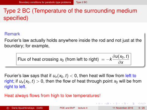
RemarkFourier’s law actually holds anywhere inside the rod and not just at theboundary; for example,
Flux of heat crossing x0 (from left to right) = −k∂u(x0, t)∂x
Fourier’s law says that if ux (x0, t) < 0, then heat will flow from left toright; if ux (x0, t) > 0, then the flow of heat through point x0 will be fromright to left.
Heat always flows from high to low temperatures!
c© Daria Apushkinskaya (UdS) PDE and BVP lecture 4 11 November 2016 9 / 29

Boundary conditions for parabolic-type problems Type 2 BC
Type 2 BC (Temperature of the surrounding mediumspecified)
Finally, combining two expressions for heat flux, we get our desiredBCs in purely mathematical terms; namely,
BCs
∂u(0, t)∂x
=hk
[u(0, t)− g1(t)]
∂u(L, t)∂x
= −hk
[u(L, t)− g2(t)]
0 < t <∞
Quite often, the constant h/k is simply written as λ.
c© Daria Apushkinskaya (UdS) PDE and BVP lecture 4 11 November 2016 10 / 29

Boundary conditions for parabolic-type problems Type 2 BC
Type 2 BC (Temperature of the surrounding mediumspecified)
In higher dimensions, we have similar BCs.
ExampleFor example, if the boundary of a circular disc is interfaced with amoving liquid that has a temperature g(θ, t), our BCs would be
∂u(R, θ, t)∂r
= −hk
[u(R, θ, t)− g(θ, t)] .
This type of BCs would be called a linear BC (since it is linear in u andur ) but nonhomogeneous due to the right-hand side g(θ, t).
c© Daria Apushkinskaya (UdS) PDE and BVP lecture 4 11 November 2016 11 / 29
Boundary conditions for parabolic-type problems Type 3 BC
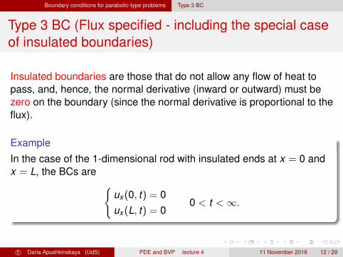
Type 3 BC (Flux specified - including the special caseof insulated boundaries)
Insulated boundaries are those that do not allow any flow of heat topass, and, hence, the normal derivative (inward or outward) must bezero on the boundary (since the normal derivative is proportional to theflux).
ExampleIn the case of the 1-dimensional rod with insulated ends at x = 0 andx = L, the BCs are {
ux (0, t) = 0ux (L, t) = 0
0 < t <∞.
c© Daria Apushkinskaya (UdS) PDE and BVP lecture 4 11 November 2016 12 / 29

Boundary conditions for parabolic-type problems Type 3 BC
Type 3 BC (Flux specified - including the special caseof insulated boundaries)
In 2-dimensional domains, an insulated boundary would mean that thenormal derivative of the temperature across the boundary is zero.
ExampleFor example, if the circular disc were insulated on the boundary, thenthe BC would be
ur (R, θ, t) = 0 ∀ 0 6 θ < 2π and ∀ 0 < t <∞.
c© Daria Apushkinskaya (UdS) PDE and BVP lecture 4 11 November 2016 13 / 29
Boundary conditions for parabolic-type problems Type 3 BC
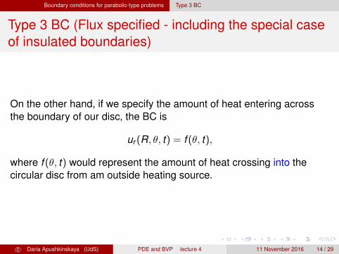
Type 3 BC (Flux specified - including the special caseof insulated boundaries)
On the other hand, if we specify the amount of heat entering acrossthe boundary of our disc, the BC is
ur (R, θ, t) = f (θ, t),
where f (θ, t) would represent the amount of heat crossing into thecircular disc from am outside heating source.
c© Daria Apushkinskaya (UdS) PDE and BVP lecture 4 11 November 2016 14 / 29

Boundary conditions for parabolic-type problems Typical BCs for 1-dimensional heat flow
Typical BCs for 1-dimensional heat flow
Let us consider the following experiment
1 Suppose we have a copper rod 200 cm long that is laterallyinsulated and has an initial temperature of 0◦C.
2 Suppose the top of the rod (x = 0) is insulated, while the bottom(x = 200) is immersed in moving water that has a constanttemperature of g(t) = 20◦C.
c© Daria Apushkinskaya (UdS) PDE and BVP lecture 4 11 November 2016 15 / 29
Boundary conditions for parabolic-type problems Typical BCs for 1-dimensional heat flow
Typical BCs for 1-dimensional heat flow
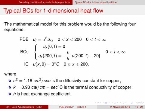
The mathematical model for this problem would be the following fourequations:
PDE ut = α2uxx 0 < x < 200 0 < t <∞
BCs
ux (0, t) = 0
ux (200, t) = −hk
[u(200, t)− 20]0 < t <∞
IC u(x ,0) = 0◦C 0 6 x 6 200,
whereα2 = 1.16 cm2/sec is the diffusivity constant for copper;k = 0.93 cal/cm − sec◦C is the termal conductivity of copper;h is heat exchange coefficient.
c© Daria Apushkinskaya (UdS) PDE and BVP lecture 4 11 November 2016 16 / 29

Boundary conditions for parabolic-type problems Typical BCs for 1-dimensional heat flow
Typical BCs for 1-dimensional heat flow
RemarkTo find h is a hard problem itself. It measures the rate that heat is beingexchanged between bottom of the rod and the surrounding water.
We would have to carry out an experiment to determine the value of h.
c© Daria Apushkinskaya (UdS) PDE and BVP lecture 4 11 November 2016 17 / 29

Derivation of the heat equation
Derivation of the heat equation
Suppose that we have a 1-dimensional rod of length L for which wemake the following assumptions:
1 The rod is made of a single homogeneous conducting material.
2 The rod is laterally insulated (heat flows only in the x-direction).
3 The rod is thin (the temperature at all points of a cross section isconstant).
c© Daria Apushkinskaya (UdS) PDE and BVP lecture 4 11 November 2016 18 / 29

Derivation of the heat equation
Derivation of the heat equation
If we apply the principle of conservation of heat to the segment[x , x + ∆x ], we can claim
Net change of heat inside [x , x + ∆x ]
= total heat generated inside [x , x + ∆x ]
+ net flux of heat across the boundaries
c© Daria Apushkinskaya (UdS) PDE and BVP lecture 4 11 November 2016 19 / 29

Derivation of the heat equation
Derivation of the heat equation
Observe that the total amount of heat (in calories) inside [x , x + ∆x ] atany time t is measured by
Total heat inside [x , x + ∆x ] =
x+∆x∫x
cρAu(s, t)ds ,
wherec = thermal capacity of the rod (measures the ability of the rod tostore heat);ρ = density of the rod;A = cross-section ares of the rod.
c© Daria Apushkinskaya (UdS) PDE and BVP lecture 4 11 November 2016 20 / 29
Derivation of the heat equation
Derivation of the heat equation
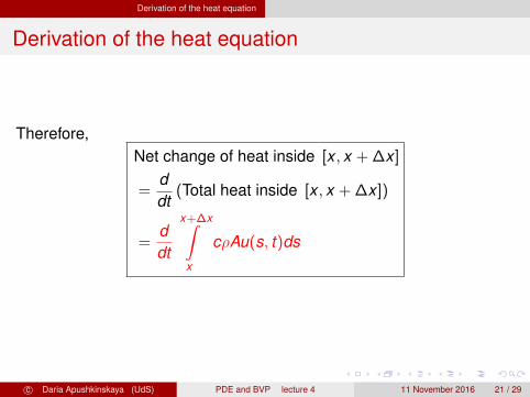
Therefore,Net change of heat inside [x , x + ∆x ]
=ddt
(Total heat inside [x , x + ∆x ])
=ddt
x+∆x∫x
cρAu(s, t)ds
c© Daria Apushkinskaya (UdS) PDE and BVP lecture 4 11 November 2016 21 / 29
Derivation of the heat equation
Derivation of the heat equation
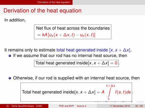
In addition,
Net flux of heat across the boundaries= kA [ux (x + ∆x , t)− ux (x , t)]
It remains only to estimate total heat generated inside [x , x + ∆x ].If we assume that our rod has no internal heat source, then
Total heat generated inside[x , x + ∆x ] = 0 .
Otherwise, if our rod is supplied with an internal heat source, then
Total heat generated inside[x , x + ∆x ] = A
x+∆x∫x
f (s, t)ds .
c© Daria Apushkinskaya (UdS) PDE and BVP lecture 4 11 November 2016 22 / 29
Derivation of the heat equation
Derivation of the heat equation
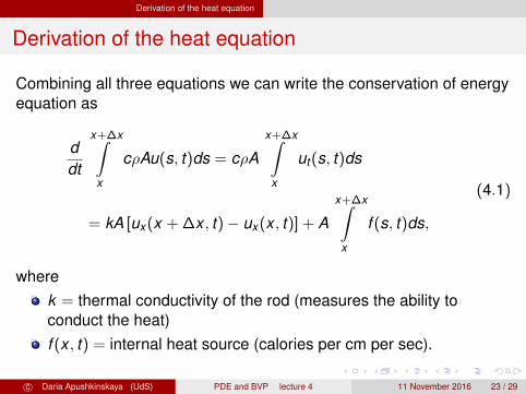
Combining all three equations we can write the conservation of energyequation as
ddt
x+∆x∫x
cρAu(s, t)ds = cρA
x+∆x∫x
ut (s, t)ds
= kA [ux (x + ∆x , t)− ux (x , t)] + A
x+∆x∫x
f (s, t)ds,
(4.1)
wherek = thermal conductivity of the rod (measures the ability toconduct the heat)f (x , t) = internal heat source (calories per cm per sec).
c© Daria Apushkinskaya (UdS) PDE and BVP lecture 4 11 November 2016 23 / 29
Derivation of the heat equation
Derivation of the heat equation
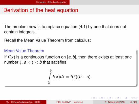
The problem now is to replace equation (4.1) by one that does notcontain integrals.
Recall the Mean Value Theorem from calculus:
Mean Value TheoremIf f (x) is a continuous function on [a,b], then there exists at least onenumber ξ, a < ξ < b that satisfies
b∫a
f (x)dx = f (ξ)(b − a).
c© Daria Apushkinskaya (UdS) PDE and BVP lecture 4 11 November 2016 24 / 29

Derivation of the heat equation
Derivation of the heat equation
Applying the Mean Value Theorem to equation (4.1) we arrive forx < ξi < x + ∆x at the following equation:
cρAut (ξ1, t)∆x = kA [ux (x + ∆x , t)− ux (x , t)] + Af (ξ2, t)∆x
or
ut (ξ, t) =kcρ
{ux (x + ∆x , t)− ux (x , t)
∆x
}+
1cρ
f (ξ, t).
c© Daria Apushkinskaya (UdS) PDE and BVP lecture 4 11 November 2016 25 / 29
Derivation of the heat equation
Derivation of the heat equation
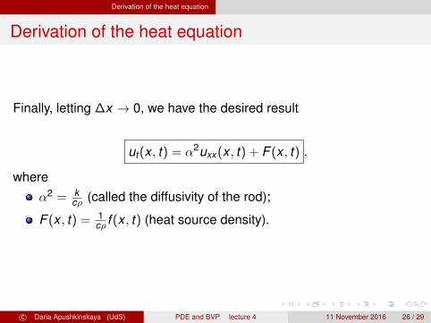
Finally, letting ∆x → 0, we have the desired result
ut (x , t) = α2uxx (x , t) + F (x , t) ,
whereα2 = k
cρ (called the diffusivity of the rod);
F (x , t) = 1cρ f (x , t) (heat source density).
c© Daria Apushkinskaya (UdS) PDE and BVP lecture 4 11 November 2016 26 / 29

Derivation of the heat equation
Derivation of the heat equation
Suppose the rod is not laterally insulated and the heat can flow acrossthe lateral boundary at a rate proportional to the differnce between thetemperature u(x , t) and the surrounding medium that we keep at zero.
In this case, the conservation of heat principle will give
ut = α2uxx − βu + F (x , t),
where β = rate constant for the lateral heat flow (β > 0).
c© Daria Apushkinskaya (UdS) PDE and BVP lecture 4 11 November 2016 27 / 29

Derivation of the heat equation
Remarks1 The constant k is the thermal conductivity of the rod and a
measure of the heat flow (in calories) that is transmitted persecond through a plate 1 cm thick across an area of 1 cm2 whenthe temperature difference is 1◦C.
2 If the material of the rod is uniform, then k will not depend on x .For some materials, the value of k depends on the temperature u.
3 The constant c is known as thermal capacity of the substance andmeasures the amount of energy the substance can store.
c© Daria Apushkinskaya (UdS) PDE and BVP lecture 4 11 November 2016 28 / 29
Derivation of the heat equation
RemarkThe units of some of the basic quantities of heat flow (in the egs.measurement system) are
u = temperature (degrees centigrade)ut = rate of change in temperature (◦C/sec)
ux = slope of temperature curve (◦C/cm)
uxx = concavity of temperature curve (◦C/cm2)
α2 = diffusivity (cm2/sec).
c© Daria Apushkinskaya (UdS) PDE and BVP lecture 4 11 November 2016 29 / 29