Transportation Research Record 1070 125

Pavement Condition Data Analysis and Modeling

MARIA MARG AR IT A NUNEZ and MOHAMED Y. SHAHIN

ABSTRACT

To maximize the benefits of pavement management, a reliable method of pavement condition forecasting is extremely important. Described is a methodology for pavement condition data analysis and a modeling technique for use in the PAVER pavement management system. The latest PAVER data bases from 18 civilian agencies and 2 military installations were used to verify this methodology. Several models were developed for each location to account for the wide variety of factors affecting pavement performance. Relevant information of the pavement sections was organized into pavement families; a family is defined by the pave­ment type, pavement rank, and pavement functional classification. A screening procedure was designed to examine the data retrieved for obvious errors. A statistical outliers analysis was implemented to detect any unusual observa­tions. The family model accepted for pavement condition index prediction was developed from the pavement AGE variable averaged every 3 years to obtain a representative point for each 3-year period. This point was then used in the final polynomial regression analysis. Pavement condition forecasting for each section was accomplished by customizing the prediction depending on the present condition in relation to the family curve. The family models were designed for continuous update as more data are gathered for a given location and entered in the PAVER data base.

Prediction of pavement performance using nondestruc­tive testing (NDT) results has been studied by O'Brien, Kohn, and Shahin (1). For model develop­ment, O'Brien et al. included several variables: pavement type, condition rating, NDT information, pavement construction, traffic information, and pavement layer thicknesses. The independent variables included in the final model for pavement condition prediction were pavement construction history, a weighted traffic variable, and NDT deflection param­eters. The pavement construction history was re­flected in three pavement layer age variables: time since last overlay, time from construction to first overlay, and total pavement age. The NDT parameters were a normalized deflection factor given by the slope of the deflection basin, and a measure of the deflection basin area. The traffic variable included in the prediction model is the natural logarithm of current traffic count weighted by traffic type {pas­senger vehicles, two-axle trucks, three or more axle trucks). The relative significance of each variable group was 60 percent for the age variables, 30 per­cent for the NOT variables, and 10 percent for the traffic variable.

The prediction model presented by O'Brien et al. was considered adequate for network condition pro­jection but not for the project-level condition pre­diction. An overall regression model based on all the variables originally included was not considered satisfactory particularly for project-level analysis. This was attributed to the complexity of accurately accounting for all variables in one model. The model was developed from data for one location; therefore climatic effects were not included. Also, the model is static in that it would be difficult for the average pavement manager user to update the model when additional pavement condition data become available.

To maximize management benefits, a reliable method

u.s. Army Construction Engineering Laboratory, P.O. Box 4005, Champaign, Ill. 61820-1305.

of pavement condition forecasting is extremely im­portant. Proper selection of an optimum maintenance strategy at the network and project levels depends on the availability of an accurate prediction model that reflects local conditions. In this paper, a methodology for pavement condition data analysis and the development of a prediction model for use in the PAVER pavement management system are described (2). In this methodology, models are developed for e~ch specific location and models are continuously updated as more data are gathered and entered in the PAVER data base.

PAVER DATA BASES

The condition rating procedure used in this study is the pavement condition index (PCI) of the PAVER pavement management system developed by the U.S. Army Construction Engineering Research Laboratory (USA-CERL) <l•l>· The PAVER system provides the user with data storage and retrieval, pavement network definition, establishment of project priorities, inspection scheduling, determination of current and future network condition, maintenance and repair needs, economic analysis, and budget planning. PCI is a composite index of the pavement's structural integrity and operating condition. PCI of a pavement section is determined based on distress type, quan­tity, and severity. It is a numerical index from 0 to 100 that has been divided into seven categories that range from failed to excellent, as shown in Figure 1.

PAVER is a pavement management system that im­proves the maintenance decision-making process at the network and project levels. The prediction meth­odology presented here and developed as part of the PAVER program can be effectively utilized by other management systems. The PAVER system has been widely implemented by many military installations and has been adopted by the American Public works Association for use by cities and counties. The latest PAVER

126

CONDITION RATING

EXCELLENT

VERY GOOD

?O - GOOD

55- FAIR

40~ POOR 25~ VERY POOR

l:0FAILEO

FIGURE 1 Pavement condition index and condition roting scale.

data bases from 18 civilian agencies (cities and counties) and military installations were used to verify the methodology presented in this paper.

Data available in PAVER for each of these agencies include pavement identification, pavement rank or functional classification (primary, secondary, etc.), condition history, layer material properties, and traffic records.

MODELING PROCEDURE

The overall procedure for model development is shown in Figure 2. By using a program developed to access the PAVER data base and retrieve information for each pavement section, it was possible to obtain data for more than 6 ,300 cases. This program takes the users' request for family definition based on the uniform conditions of the pavement sections and prints information pertinent to pavement identifica­tion, pavement condition, time since the pavement was built or last reconstructed, pavement structure, layer material properties, and traffic. Although the data retrieved are sufficient for family definition, most of the information currently stored in the PAVER

No

Mode l Development

Pavement Condition

Forecasling

PAVER Data Base

Doto Ret r ievol By Family

FIGURE 2 Flow diagram of modeling procedure.

Transportation Research Record 1070

data bases pertains to a one-time survey for each section during the lifetime of the pavement. To en­sure adequate model development, it would have been desirable to have replicate measurements of pavement field condition and also information for different time periods.

Information on several pavement sections was found to be in error; these errors originated during data collection, coding, or entering in the data base. A screening program that examines the data retrieved for obvious errors was also developed, as explained in a subsequent section of this paper. As shown in the flow diagram in Figure 2, screened data are also examined for outliers that may have a great influence in the model selection phase. A model for pavement condition prediction is developed for each family of pavements, in which the data are averaged every 3 years to obtain a representative point for each 3-year period. The selection of the best prediction model for mathematical condition is based on mini­mizing prediction errors, as explained later. Fi­nally, Pt:! prediction of a given section is deter­mined by modifying the prediction curve, depending on the section's present condition relative to the prediction model curve for the pavement family.

CONCEPT OF PAVEMENT FAMILIES

More than one model should exist for a given location to account for the wide variety of factors affecting pavement performance. Therefore, a model should be developed for each family of pavements at each pave­ment location. Relevant information elements of the pavement sections in the PAVER data bases have been reorganized into pavement family files in which every family is defined by the pavement type, pavement use, and the pavement rank or functional classification. Grouping pavement sections with similar characteris­tics makes it possible to develop relationships for prediction at an acceptable level of confidence.

The several choices for the selection of a pave­ment family are as follows:

• Pavement type: asphalt concrete (AC) , port­land cement concrete, (PCC), asphalt concrete over­lay on portland cement concrete (APC), and asphalt concrete overlay on asphalt concrete (AAC);

• Pavement use, which is identified by the ser­vice rendered, such as roadways, streets, parking lots, runways, taxiways, or aprons; and

• Pavement rank or functional classification, such as arterials (primary), collectors (secondary), and local roads and streets (tertiary) •

The data collection summary for roadways (by pave­ment family) is given in Table 1 for original pave­ments (without overlay) and in Table 2 for overlaid pavements. The tables include data from 15 data banks and 94 families for a total of more than 6,300 cases.

DATA SCREENING PROCEDURE

Errors have been identified as those pieces of data in which a mistake was comrni tted when gathering, coding, or entering the data. Pieces of inaccurate data can be found because they break basic system rules; examples are PCI values greater than 100 when the PCI scale is from 0 to 100, or two identical AGE records that show different PCis. One of the assump­tions of this modeling technique is that a section of pavement deteriorates with time at different rates during the life of the pavement; therefore, to eliminate obvious errors but not questionable data the methodology allows the user to define data

Nunez and Shahin

TABLE 1 Data Collection Summary for Original Pavements by Pavement Rank for Two Surface Types

AC PCC

Base Principal Arterial Collector Industrial Residential Principal Arterial Collector Industrial Residential

Ada Co., Idaho 100 110 140 148 188 Abilene, Texas 1S9 S3 2 Bellingham, Washington Billings, Montana 2 16 7S Bloomingdale, Illinois 7 12 119 2S Bryan, Texas 9 17 128 131 4 26 19 Calgary, Canada 693 4 Glenn Ellyn, Illinois IS 2S 120 3 Hayward, California so 22 S6S Niagara, Canada 614 3 Overland Park, Kansas Ill 194 Tacoma, Washington 66 so SS 3 2 9 7 16 Winnipeg, Canada 4 Fort Eustis, Virginia 2 4 13 3 4 18 Great Lakes, Illinois 21 109 72 2 4 12

Note: AC is asphalt concrete and PCC is portland cement concrete. The numbers in each cell indicate the number of cases in that family.

TABLE 2 Data Collection Summary for Overlaid Pavements by Pavement Rank for Two Surface Types

AC/AC AC/PCC

Base Principal Arterial Collector Industrial Residential Principal Arterial Collector Industrial Residential

Ada Co., Idaho 17 10 12 2 2 Abilene, Texas Bellingham, Washington 31 22 2S 183 2 Billings, Montana Bloomingdale, Illnois Bryan, Texas Calgary, Canada 194 Glenn Ellyn, Illinois 8 22 78 Hayward, California 82 42 47S Niagara, Canada Overland Park, Kansas Tacoma, Washington 30 3S 30 9 2 Winnipeg, Canada 109 Fort Eustis, Virginia 44 36 93 2 2 Great Lakes, Illinois 36 104 9S 37 so 17

Note: AC is asphalt concrete and PCC is portland cement concrete. The numbers in each cell indicate the number of cases in that family.

boundaries. The questionable data are analyzed in a separate part of this methodology under outliers identification.

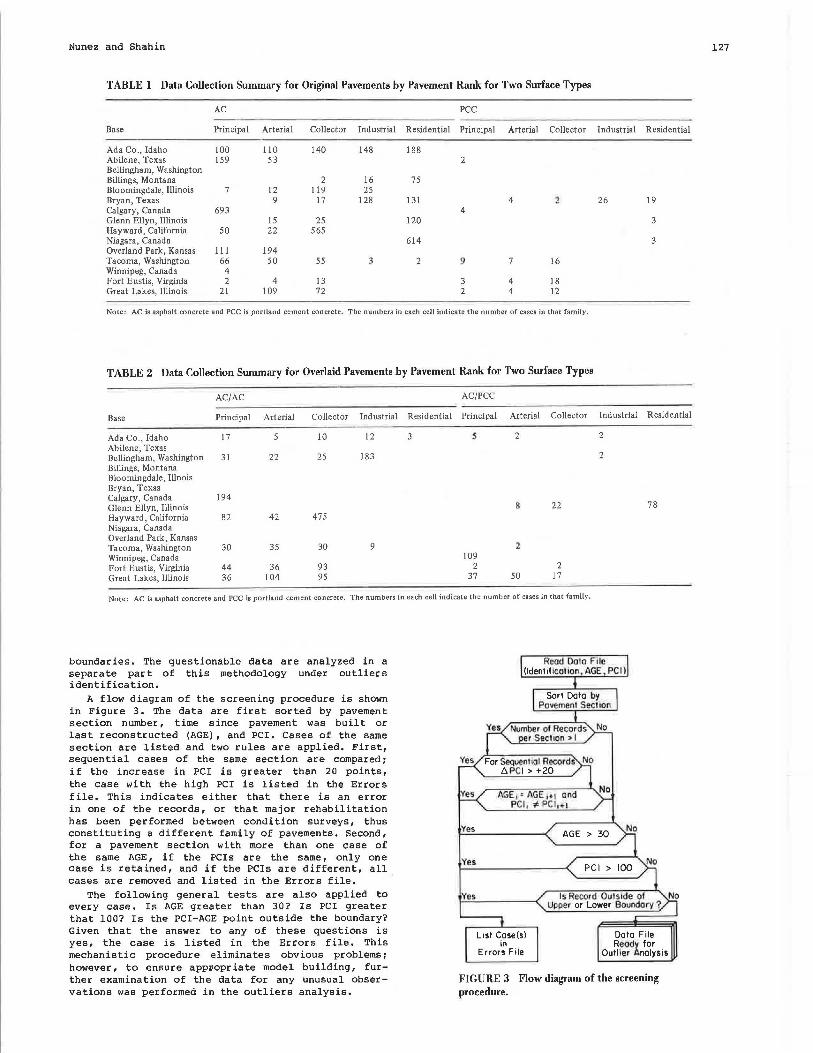
A flow diagram of the screening procedure is shown in Figure 3. The data are first sorted by pavement section number, time since pavement was built or last reconstructed (AGE), and PCI. Cases of the same section are listed and two rules are applied. First, sequential cases of the same section are compared; if the increase in PC! is greater than 20 points, the case with the high PC! is listed in the Errors file. This indicates either that there is an error in one of the records, or that major rehabilitation has been performed between condition surveys, thus constituting a different family of pavements. Second, for a pavement section with more than one case of the same AGE, if the PCis are the same, only one case is retained, and if the PCis are different, all cases are removed and listed in the Errors file.

The following general tests are also applied to every case. Is AGE greater than 30? Is PC! greater that 100? Is the PCI-AGE point outside the boundary? Given that the answer to any of these questions is yes, the case is listed in the Errors file. This mechanistic procedure eliminates obvious problems; however, to ensure app1mpr iate model building, fur­ther examination of the data for any unusual obser­vations was performed in the outliers analysis.

Read Da to Flle (ldentif1cot1on, AGE PCll

Sort Octa by Pavement Section

Yes For Sequen11al Records 6 PC I > +20

Yes AGE 1 = AGE 1+1 and

Yes

Yes

Yes

PC l 1 'F- PC l 1+·1

List Case(s) in

Errors File

AGE > 30 No

PCI > 100

Is Record Outside of Upper or Lawer Boundary?

Doto File Ready for

Outl ier Analysis

FIGURE 3 Flow diagram of the screening procedure.

127

128

OUTLIERS ANALYSIS

Cases with unusual values can have substantial impact in the statistical analysis of pavement condition modeling of a family. Therefore, to identify data with very large or very small values, every family file was subjected to an analysis of residuals based on linear regression analysis. The rate of deterio­ration, which represents the reduction in PCI over a given time period, was initially included for out-1 iers identification. The frequency distribution of the rate of deterioration was plotted and found to be skewed to the left, that is, the concentration of the rate of deterioration values was greatest around the lower rate of deterioration. Therefore, setting a confidence interval for data screening based on the rate of deterioration was not possible because data points with very low rates of deterioration could not be observed.

A technique for outliers identification based on residuals analysis was then applied to the data. Residuals are calculated as the difference between the observed value and the value predicted by a linear regression model of PCI against AGE. The fre-

SHOW. INCLUDE 'C:\SPSS\DATA\2ADACA.FIL'. DATA LIST FILE= ' \SPSS\DATA\2ADACA.PRN ' /

AGE 1-6 (3) PCI 7-10.

Transportation Research Record 1070

quency distribution of residuals was found to be normal, thus lending itself to setting confidence intervals. This is always the case with the residuals frequency plot even if the distribution of the com­ponents is markedly nonnormal (3). The standard de­viation of the residuals was used as a measure of spread to observe the relative magnitude of any par­ticular residual.

The regression subprogram of the Statistical Package for the Social Sciences (SPSS) software for personal computers was used to find the best-fit mathematical function between PCI as the dependent variable and AGE as the independent variable Ci>· A sample output of the regression analysis using SPSS is shown in Figure 4. A straight-line function ob­tained by the least-squares analysis was used to predict PCI values. After building an equation, sev­eral types of residuals and related statistics were requested from the analysis of residuals feature of SPSS. These residuals were used to locate outliers and examine basic regression assumptions. A list of the 10 most extreme normalized residuals wall yener­ated along with a histogram of normalized residuals. The normal probability of the residuals and cases

VARIABLE LABELS AGE 'TIME SINCE LAST DAY OF CONSTRUCTION ' PCI 'PAVEMENl CONDITION INDEX'.

REGRESSION VARIABLES AGE PCI I The raw data or transformation pass is proceeding SPSS/PC has written 99 cases to the active file STATISTICS = SES DEFAULTS/ DEPENDENT = PCI/ METHOD = ENTER AGE/ RESIDUALS = ID (AGE) DEFAULTS.

Page 2 SPSS/PC Relea&e 1.10 2/11/86

* * * * M U L T I P L E R E G R E S S I 0 N * * * *

Listwise Deletion of Missing Data

Equation Number Dependent Variable •. PCI PAVEMENT CONDITION INDEX

Beginning Block Number 1. Method: Enter AGE

Variable(s) Entered on Step Number 1.. AGE TIME SINCE LAST DAY OF CONSTRUCTION

Multiµle R .43175 R Square .18641 Adjusted R Square .17802 Standard Error 13.91469

Analysis of Variance

Regression Residual

OF 1

97

Sum of Squares 4303.08850

18780.99231

F = 22.22458 Signif F = .0000

M&!an Square 4303.08850

193.61848

- - - --- --------------- Variables in the Equation

Variable

AGE <Constant>

B

-1.05768 73.75811

End Block Number

SE B

. 224::;6 3.07865

Beta

-.43175

SE Beta

.09158

All requested variables entered.

FIGURE 4 Sample output of the regression analysis using SPSS.

T Sig T

-4.714 .0000 23.958 .0000

Page 3 SPSS/PC Release 1.10 2/11/86

* * * * M U L T I P L E R E G R E S S I 0 N * * * *

Equation Number 1 Dependent Variable .• PCI PAVEMENT CONDITION INDEX

Residuals Statistics:

MIN MAX MEAN STD DEV N *PRED 44.0552 72.6126 60.8283 6.6264 99 *RES ID -30.2089 28.7069 -.oooo 13.8435 99 *ZPRED -2.5313 1.7784 .0000 1. 0000 99 *ZRESID -2.1710 2.0631 -.0000 .9949 99

Total Cases 99

Durbin-Watson Test 1.56509

* * * * * * * * * * * * * * * * * * * * * * * * * * * * * Outliers - Standardized Residual

Case # AGE *ZRESID 23 8.083 -2.17101 40 5.167 2.06307 78 2.083 1.90051 29 6.917 -1.90030 56 2.000 1.89420 57 17.000 -1.85254 39 5.167 1.84747 15 14.000 -1. 79311

7 24.083 1. 77612 47 21. 167 1.77006

Page 4 SPSS/PC Release 1.10

Histogram - Standardized Residual

NExp N (* = 1 Cases, : Normal Curve) 0 .08 0L1t 0 . 15 3.00 0 .39 2.67 0 • 88 2.3~ . 4 1. 81 2.00 *=** 6 3. ~;1 1. 67 *M-=*** 4 5.43 1. 33 ****· 7 7.98 1 . 00 *******· 9 1 o. 5 .67 ********* * 12.4 .33 ******* ** * 13. 1 o. (I ************=** * 12.4 -.33 ***********· * 10. 5 -.67 **********•* 8 7.98 -1. 00 *******• 8 5.43 -1.33 ****•*** 2 :3 . 31 -1.67 **· 2 1. 81 -2 .. 00 ... ,

.88 -·2 . 33 0 .39 -2.67 (l .15 -3.00 0 . 08 Out

* * * * * * * * * * * * * * * * * * * * * * * * * * * * * Normal Probability CP-P> Plot Standardized Residual

1.0 EDDDDDDDDDEDDDDDDDDDEDDDDDVDDVEVDDDDDDV** .J 3 3 *** .J .J ** 3 .3 *** 3

.75 E ** E 3 ** 3

0 3 ** .J

b 3 *** .3 s .3 **· .J

e .5 E *· E r .3 ** .3 v 3 * .3 e .J **** .J d .3 *· .J

.25 E ** E 3 ** 3 .3 ** .J .3 * 3 3 ** 3 E*DDDDDDDDEDDDDDDDDDEDDDDDDDDDEDDDDDDDDDE Expected

•>e oLu

e ·'"' .75 1.0

FIGURE 4 (continued)

2/11/86

130

that fall outside the normal curve were identified. The probability that a deviation in either direction will exceed three standard deviations is close to zero. Therefore, any deviation larger than three standard deviations was assumed to be out of the expected values and the case was listed as an out­lier. The selection of three standard deviations for outliers may be ultraconservative and thus a normal probability value of 2.5 may be used for outlier analysis.

MODEL DEVELOPMENT

Preliminary analysis and results from previous studies (1) have shown that PCI is strongly related to AGE for a given pavement family and that no sig­nificant correlation can be found with the other data base variables, given that families of pavements were correctly defined. For example, runways and aprons were not combined in one family. Therefore, linear regression models and hi-order polynomial regrcooion cquationo for PCI prediction as a function of AGE were investigated for their use in this re­search project.

After errors and outliers were eliminated from the data files, model development for each family followed. The first approach attempted for PCI fore­casting was stepwise regression using the SPSS <!> • A scattergram of the PCI and AGE variables was examined. The plot revealed a curvilinear relation­ship between the variables. This can be observed in Figures 5-7, in which PCI is plotted as a function of AGE for three different families . Although it was clear that the relationship between AGE and PCI fol­lows a curve of second or third order, the least­squares stepwise regression method was always se­lecting a straight-line regression equation as the best fitting model. This was attributed to the im­balance of the number of cases in each pavement category and the inability of regression models to explain inflection points, as demonstrated by the figures.

The stepwise regression method is the best vari-

PAVEMENT CONDITION INDEX (PCI) IOOr---:-..-~-.-~-.-~-r~---.~~.--~...-~...,....~--.-~-.

90 •• eo

70 •

so- .. : . 50 ...

. 40>-

30

20

10 >-

.. . •• . . . . ' .. .. . . · .. . .. .

. . .. \. · ... . .

••• . . I .

•I . . .

0 I I I I I I I I I 0~~3:;-~6~~9,:--~~,2~~1~~~18~~2~1~-2~4~-2~7~-'30

PAVEMENT AGE IN YEARS

FIGURE 5 Scatterplot of PCI versus AGE for an AC surface pavement-primary road family.

able selection procedure: it is fast and works with one independent variable at a time while improving the equation at every step. However, stepwise re­gression makes an automatic insertion of a variable determined by a test of significance, and judgment is still required in the examination of the final mOdel (~).

Because a polynomial function based on stepwise regression could not be obtained for any family, the data were divided in two groups, one for pavement

Transportation Research Record 1070

PAVEMENT CONDITION INDEX (PCI) 1001~~~.--~~r-~~..-~~-.-~~-r-~~-.

so -70 -

60

50 -

40 -

30 -

20 -

10 >-

00 I

3

• • . •

I

6 9 12 15 PAVEMENT AGE IN YEARS

FIGURE 6 Scatterplot of PCI versus AGE for an AC surface pavement-tertiary road family.

PAVEMENT CONDITION INDEX (PCI)

18

100..-.....---.~.,...,.~...---.-~.---.-~~-.-----.~-.---.~...--r~ • 90 -·

80

70

60

50

40

30

20

10

• • • • • •

.-• ( • •

• • • •

% 369~~~~M~~~~~G~ PAVEMENT AGE IN YEARS

FIGURE 7 Scatterplot of PCI versus AGE for an AC/AC surface pavement-secondary road family.

sections with a PCI of from 0 to 60 and the other for sections with a PCI of from 61 to 100. A PCI of 60 was assumed to represent the main inflection point in a PCI versus AGE curve. Multiple regression anal­ysis was then performed for both groups and a curve of the desirable shape was found for each group of data. However, this procedure could not be used as an overall prediction model because the curves did not converge at the PCI point of 60, preventing the creation of a continuous curve for PCI prediction that would describe the total range of AGE •

The data were then grouped for different AGE ranges and the best regression line was fitted through points that represented the average of each group. This was done under the assumption that the average pavement condition in a given AGE range weighs equally regardless of the number of points existing in a given range. By grouping the data for AGE ranges of 3 years, a third-order polynomial could easily be fitted. This is shown in Figures 8, 9, and 10, in which third-degree polynomials were fitted for the data shown in Fi gures 5, 6, and 7, respec­tively.

To obtain a measure of the acceptability of this relationship, the mean squares (MS) of the devia­tions of the observed Yi from the predicted Yi by mc>dels representing first-, second-, and third-order polynomials were compared, as shown in Table 3. The root mean squares (RMSs) calculated as the square root of MS divided by the sample size is always lower for the third-order polynomial, thus showing the advantage of choosing a third-degree polynomial for modeling PCI-AGE of a given pavement family.

Nunez and Shahin

PAVEMENT CONDITION INDEX (PCI) 100.-~..-~-.-~-.-~-..~~.--~..-~-.-~-.-~ ........ ~--.,

70

60 -

50-

40

30 -

20

10

00 3 6

• AGE RANGE • 3

9 12 15 18 21 24 27 PAVEMENT AGE IN YEARS

FIGURE 8 Third-order polynomial regression for an AC surface pavement-primary road family.

PAVEMENT CONDITION INDEX (PCI)

30

IOOr-~~-.--~~-.~~~-.-~~-.~~~-..--~~-.

90 -• AGE RANGE • 3 eo,__ _ __ _

70

60

50

40

30

20

10

00~~~-3~~~~6~~~~9~~~~12~~~~15~~--..15

PAVEMENT AGE IN YEARS

FIGURE 9 Third-order polynomial regression for an AC surface pavement-tertiary road family.

PAVEMENT CONDITION INDEX (PCI) 100.---.---.-~.--.---.~-..---.-----,.---.---..~.--.--.~-..---.

90

BO -

70

60

50

40

30

20

10

• AGE RANGE• 3

oO 3 6 9 12 15 16 21 24 27 30 33 36 39 42 45 PAVEMENT AGE IN YEARS

FIGURE 10 Third-order polynomial regression for an AC/AC surface pavement-secondary road family.

PAVEMENT CONDITION FORECASTING

The prediction models were developed to represent the average behavior of an entire pavement family. Therefore, PCI prediction for each section should be modified depending on its relative position to the curve. To predict the future PCI of a section, a curve is drawn through the present PCI-AGE point, which is parallel to the prediction model curve for the pavement family at equal condition. The PCI can then be determined at the desired future AGE by reading from the later curve. This is shown in Fig-

TABLE 3 Comparison of Root Mean Squares

Order of Polynomial Line

Family

AC pavement, primary road AC pavement, tertiary road AC/AC pavement, secondary road

40

30 -

20 -

10

00 5 10 15

First

14. 11 14.37 14.47

20 TIME IN YEARS

Second

13.75 12.94 14.48

25

Third

13.11 12.88 14.37

30

FIGURE 11 Example of pavement condition forecasting.

131

ure 11, in which a given section of the road pre­sented by the dot is 10 years old with a PCI of 70. By drawing curve parallel to the family curve through the point and looking for the pavement condition at year 20, PCI is predicted to be 56 within 10 years.

In this technique, it is assumed that the deterio­ration of pavements is a function of their present condition regardless of AGE. Therefore, the technique is likely to produce more accurate results for short-term prediction than for long range (i.e., 20 years). Because budget planning for maintenance and repair is usually prepared for a 5-year period, and because the models are continuously updated when new condition data are made available, this technique is expected to yield acceptable results at the network and project levels. Other techniques are also cur­rently being investigated by USA-CERL and will be reported on in the future.

SUMMARY

Data available in the PAVER pavement management sys­tem were used in the form of pavement families for outlier analysis and modeling of pavement condition. A pavement family is defined by pavement type, pave­ment use, and pavement rank or functional classifi­cation. Grouping of pavement sections by their similar conditions made it possible to develop rela­tionships for prediction at an acceptable level.

A screening procedure was designed to clean the data of each family from obvious errors. To ensure appropriate model building, a statistical outliers analysis was also developed. The outliers procedure is based on an examination of the residuals of a straight-line regression model. For pavement condi­tion model development, the AGE data were averaged every 3 years to obtain a representative point for each 3-year period. This point was then used in the final polynomial regression analysis. Pavement con­dition forecasting was accomplished by customizing the prediction for each individual section depend­ing on its condition in relation to the prediction model curve for the pavement family. The family models were designed to be easily updated by PAVER

132

users when new pavement condition data are entered to their PAVER data bases.

REFERENCES

1. D.E. O'Brien, S.D. Kohn, and M.Y. Shahin. Pre­diction of Pavement Performance by Using Non­destructive Test Results. In Transportation Re­search Record 943, TRB;-- National Research Council, Washington, D.C., 1983, pp. 13-17.

2 . M.Y. Shahin and S.D. Kohn. Pavement Maintenance Management for Roads and Parking Lots. Technical Report M-294. Construction Engineering Research Laboratory, U.S. Army Corps of Engineers, Champaign, Ill., Oct. 1981.

3. D.V. Huntsberger and P. Billingsley. Elements of

Transportation Research Record 1070

Statistical Inference. Allyn and Bacon, Inc., March 1979, 4th ea.

4 . M.J. Norusis. Statistical Package for the Social Sciences (SPSS/ PC for the IBM/XT) • SPSS Inc., Chicago, Ill., 1984, 624 pp.

5. N.R. Draper and H. Smith. Applied Regression Analysis. Wiley Series in Probability and Mathe­matical Statistics, New York, Jan. 1981, 2nd ea.

The views of the authors do not purport to reflect the position of the Department of the Army or the Department of Defense.

Publication of this paper sponsored by Committee on Monitoring, Evaluation and Data Storage.

Use of Surface Waves 1n Pavement Evaluation

SOHEIL NAZARIAN and KENNETH H. STOKOE II

ABSTRACT

Material characterization of pavement systems in situ is required for determining load capacity and assessing the performance and possible need for rehabilitation or replacement of the system. Nondestructive tests are usually carried out for this purpose. Desirable features of nondestructive tests are speed of operation, economy, and a sound theoretical basis compatible with the in situ data collection procedure. The most popular methods in this category are the falling weight de­f lectometer (FWD) and the Dynaflect. These methods are fast for in situ data col­lection; however, a rigorous data-reduction algorithm that can result in a unique solution and take into account the effect of the dynamic nature of the load has only begun to be developed. An alternative method of nondestructive testing has been under continuous development at the University of Texas. This method is called the spectral-analysis-of-surface-waves (SASW) method and is based on the theory of stress waves propagating in elastic media. The SASW method can be uti­lized to determine Young's modulus profiles of the pavement structure and under­lying soil as well as the thickness of each layer. In this paper the theoretical aspects of the SASW method are discussed in detail. The experimental procedure is included only briefly because it has been presented comprehensively in ear lier papers. Several case studies on different types of pavements with various thick­nesses are presented to demonstrate the utility and versatility of the SASW method. In each case, the results are compared with those of the well-established crosshole seismic test that was performed at the same locations . The Young's modulus profiles from these two independent methods compare closely.

The spectral-analysis-of-surface-waves (SASW) method of testing pavements in situ has been under develop­ment at the University of Texas since 1980. The ob­jectives of performing SASW tests are to determine elastic moduli and thicknesses of the different layers nondestructively and rapidly. The method is based on generation and detection of stress waves, specifically surface waves. The theory of elastic

University of Texas at Austin, Austin, Tex. 78712.

waves in layered media is utilized to reduce and analyze data collected in the field.

The practical aspects of the SASW method have been presented by Heisey et al. !!.l , Nazarian et al. <.~.> , and Nazarian and Stokoe (3). This paper concentrates on the theoretical aspects of the method. First, a brief background of the theory of wave propagation in an elastic, solid medium is discussed. The dis­persion characteristics of surface waves, the basis for the SASW method, are presented. Data collection and reduction are then discussed. Finally, two case