Review of QSAR Models for Ready Biodegradation

Manuela Pavan and Andrew P. Worth

2006 EUR 22355 EN

EUROPEAN COMMISSION DIRECTORATE GENERAL JOINT RESEARCH CENTRE

Institute for Health and Consumer Protection Toxicology and Chemical Substances Unit European Chemicals Bureau I-21020 Ispra (VA) Italy

Review of QSAR Models for Ready Biodegradation

Manuela Pavan and Andrew P. Worth

2006 EUR 22355 EN

The mission of the IHCP is to provide scientific support to the development and implementation of EU policies related to health and consumer protection.

European Commission Directorate – General Joint Research Centre Institute for Health and Consumer Protection

Contact information

Address: E. Fermi, 1, 21020-Ispra (VA) Italy E-mail: manuela.pavan@jrc.it

Tel.: +39 0 332 78 6201 Fax: +39 0 332 78 6717

http:// http://ecb.jrc.it/QSAR/

http:// ihcp.jrc.cec.eu.int http://www.jrc.cec.eu.int

LEGAL NOTICE

Neither the European Commission nor any person acting on behalf of the Commission is responsible for

the use which might be made of this publication.

A great deal of additional information on the European Union is available on the Internet. It can be accessed through the Europa server

(http://europa.eu.int)

EUR 22355 EN ISSN 1018-5593

© European Communities, 2006 Reproduction is authorised provided the source is acknowledged

Printed in Italy

ABSTRACT

Many regulatory laws resulting from the enactment of the United Nations Stockholm

Convention in May 2004, together with the new REACH legislation, have promoted

significant new activity in the assessment of Persistent, Bioaccumulative and Toxic

(PBT) substances. These are chemicals that have the potential to persist in the

environment, accumulate within the tissues of living organisms and, in the case of

chemicals categorised as PBTs, show adverse effects following long-term exposure.

Under REACH, estimated data generated by (Q)SARs may be used both as a

substitute for experimental data, and as a supplement to experimental data in weight-

of-evidence approaches. It is foreseen that (Q)SARs will be used for the three main

regulatory goals of hazard assessment, risk assessment and PBT/vPvB assessment. In

the Registration process under REACH, the registrant will be able to use (Q)SAR

data in the registration dossier, provided that adequate documentation is given to

argue for the validity of the model(s) used. The experimental determination of the

persistence, bioconcentration and toxicity is generally expensive and demanding to

perform. For this reason, measuring experimentally the potential PBT profiles of

those chemicals that are of potential regulatory interest is considered not feasible.

The limited empirical data, the high test costs together with the regulatory constraints

and the international push for reduced animal testing motivates a greater reliance on

QSAR models in PBT assessment.

This report provides an overview of PBT regulations and criteria, and gives a detailed

review of QSAR for estimating the biodegradation of chemicals. The role of

biotransformation in the modelling of PBT substances is also described.

CONTENTS

1. INTRODUCTION 1

2. PBT SUBSTANCES: DEFINITIONS 3 2.1 Persistence 3 2.2 Bioaccumulation / Bioconcentration 4 2.3 Toxicity 5

3. REVIEW OF PBT REGULATIONS 6 3.1 Stockholm Convention 6 3.2 OSPAR Convention 7 3.3 North American Regional Action Plans (NARAPs) 8 3.4 EU Water Framework Directive (2000/60/EC) 9 3.5 EU REACH programme 10 3.6 US EPA PBT Profiler 14 3.7 Canadian Domestic Substances List categorisation 15 3.8 PBT Japanese chemical legislation 17

4. OVERVIEW OF PBT AND vPvB CRITERIA 18 4.1. REACH PBT criteria 21 4.2. REACH vPvB criteria 22

5. METHODS FOR PBT DATA GENERATION 23 5.1 Persistence data generation 23

5.1.1 Biodegradation data 25 5.2 Bioaccumulation data generation 26 5.3 Toxicity data generation 28

6. BIODEGRADATION DATABASES 29 6.1 BIODEG Database 29 6.2 BIOLOG Database 29 6.3 MITI Database 30 6.4 ESIS Database 30 6.5 University of Minnesota Biocatalysis/Biodegradation Database (UM-BBD) 31 6.6 California Department of Food and Agriculture Biodegradation Database 31

7. QSARS FOR BIODEGRADATION 32 7.1 Group contribution approaches 37

7.1.1 Degner et al. OECD hierarchical model approach 37 7.1.2 Multivariate Partial Least Squares (PLS) model 38 7.1.3 Biodegradation Probability Program BIOWIN 40

7.1.3.1 Linear and Non-Linear Biodegradation Model 41 7.1.3.2 Ultimate and Primary Biodegradation Model 43 7.1.3.3 Linear and Nonlinear MITI Biodegradation Model 43

7.1.4 MultiCASE anaerobic program 45 7.2 Biodegradation model based on diverse theoretical descriptors 47 7.3 Expert system approaches 48

7.3.1 Inductive machine learning method 48 7.3.2 BESS 49

7.3.3 MultiCASE / META biodegradability 50 7.3.4 CATABOL probabilistic assessment of biodegradability 51 7.3.5 TOPKAT 56

7.4 TGD models for persistence 57

8. VALIDATION STUDIES ON BIODEGRADATION MODELS 59 8.1 BIODEG/PLS/MultiCASE/ Machine learning method validation on MITI-I 59

8.1.1 BIODEG validation 59 8.1.2 PLS biodegradation model validation 60 8.1.3 MultiCASE model validation 62 8.1.4 Machine learning model validation 64

8.2 BIODEG/PLS/MultiCASE validation on HPVC 64 8.3 BIODEG/OECD/PLS/MultiCASE validation on 894 MITI-I test 65 8.4 BIOWIN/PLS/MultiCASE/CATABOL validation performance comparison 67 8.5 CATABOL validation on chemicals under the Japanese Chemical Substances

Control Law 68

9. CONCLUSIONS 70

10. REFERENCES 72

LIST OF ABBREVIATIONS

AQUIRE AQUatic toxicity Information REtrieval system B Bioaccumulation BAF Bioaccumulation Factor BCF Bioconcentration Factor CAS Chemical Abstracts Service C&L Classification and Labelling CEPA Canadian Environmental Protection Act CIS Chemical Information System COMMPS Combined Monitoring-based and Modelling-based Priority Setting CSCL Chemical Substances Control Law (Japan) CTV Critical Toxicity Value DSL Domestic Substances List (Canada) EC European Commission EEV Estimated Exposure Value EFDB Environmental Fate Database (by SRC) EINECS European Inventory of Existing Commercial chemical Substances ELINCS European List of Notified Chemical Substances ENEV Estimated No Effects Value EPA Environmental Protection Agency ESIS European chemical Substances Information System ESR Existing Substances Regulation (European Union) EU European Union EURAM EU Ranking Method GA Genetic Algorithm HPVC High Production Volume Chemical Kow Octanol-water partition coefficient LPVC Low Production Volume Chemical LRT Long-Range Transport MITI Ministry of International Trade and Industry NACEC North American Commission for Environmental Co-operation NARAP North American Regional Action Plan NLP No-Longer Polymers OECD Organisation for Economic Cooperation and Development OPPT Office of Pollution Prevention and Toxics (U.S. EPA) OSPAR Oslo-Paris Convention PMN Premanufacture Notice (U.S. EPA) POP Persistent Organic Pollutant PBiT Persistent Bio-accumulating and inherently Toxic chemical PBT Persistent Bio-accumulating Toxic chemical QSAR Quantitative Structure-Activity Relationship QSPR Quantitative Structure-Property Relationship Q2ext Explained variance in prediction calculated by external validation REACH Registration, Evaluation, Authorisation of Chemicals (European Union) RTECS Registry of Toxic Effects of Chemical Substances RMSE Root Mean Squared Error R2 Coefficient of determination

s Standard error of the estimate SD Standard Deviation SMOC Sound Management of Chemicals SRC Syracuse Research Corporation TC NES Technical Committee on New and Existing Substances (European

Union) TGD Technical Guidance Document TRI Toxic Chemical Release Inventory TSCA Toxic Substances Control Act (U.S. EPA) TSMP Toxic Substances Management Policy UM-BBD University of Minnesota Biocatalysis/Biodegradation Database UNEP United Nations Environment Programme vPvB very Persistent very Bioaccumulative WFD Water Framework Directive

1

1. INTRODUCTION

Persistent, bioaccumulative, and toxic chemicals (PBTs) are the subject of several

national, and international effort to limit their production, and use.

PBT chemicals exhibit low water solubility and high lipid solubility, leading to their

high potential for bioaccumulation. In addition, multimedia releases and volatility

lead to long range environmental transport both via water and the atmosphere,

resulting in widespread environmental contamination of ecosystems and organisms,

including humans.

The possible effects of long term and cumulative exposure to such chemicals is not

always addressed adequately in risk assessment methods that base the evaluation on

acute toxicity and short term exposure. As a subgroup of PBT (Persistent,

Bioaccumulating and Toxic) substances, Persistent Organic Pollutants (POP) are of

global concern as these substances are not only extremely persistent and

bioaccumulating but they can also be transported in the air or other environmental

media far from their sources. POPs and PBTs have become the subject of growing

attention and risk management measures all over the world. The UNEP (United

Nations Environment Programme) global Stockholm Convention addressed POPs

and aimed at elimination of the releases of the listed POP substances. Moreover, it

provided a general obligation to take measures to prevent production and use of new

substances that exhibit the characteristics of POPs and it established internationally

agreed screening criteria for POPs. The Convention included a procedure for

identifying new POPs to be put under global control. One of the criteria for

persistence and long-range transport (LRT) is "scientific evidence", which can

include model calculations. Quantitative structure-activity relationship (QSAR)

models have been identified, both in scientific and policy communities, as a

prominent tool for providing such evidence. The scientific and regulatory issues for

PBTs require the identification of chemicals having these undesirable properties, and

the assignment of priority to such groups.

On 29 October 2003, the European Commission (EC) adopted a legislative proposal

[1] for a new chemical management system called REACH (Registration, Evaluation

and Authorisation of Chemicals), intended to harmonise the information

2

requirements applied to New and Existing Chemicals. The REACH Regulation, aims

among other things at identifying, evaluating and regulating PBT substances

effectively. To this end, it establishes clear criteria for the PBT properties of

chemicals.

Annex XI of the legislative proposal for REACH provides for the use of valid

(Q)SARs for predicting the environmental and toxicological properties of chemicals,

in the interests of time- and cost-effectiveness and animal welfare. An increased use

of quantitative structure–activity relationship (QSAR) models is thus foreseen for the

hazard and risk assessment of chemicals in the European Union [2].

The purpose of this report is to review available QSAR models that could be used to

estimate chemical biodegradability. This report also discusses how QSAR models

can be used to provide reliable predictions of biodegradation in support of the

identification and characterisation of PBTs, and highlights how these estimates can

be used for regulatory and non-regulatory purposes.

A concise summary of the main concepts and terminology used in the PBT field is

provided together with a short section on a persistence testing strategy accepted in

international and national programmes.

3

2. PBT SUBSTANCES: DEFINITIONS

Persistent Organic Pollutants (POPs) and Persistent, Bioaccumulative and Toxic

(PBT) substances are carbon-based chemicals that resist degradation in the

environment and accumulate in the tissues of living organisms, where they can

produce undesirable effects on human health or the environment at certain exposure

levels.

2.1 Persistence

The persistence of a substance is the length of time that a substance remains in a

particular environment before it is physically transported to another compartment

and/or chemically or biologically transformed [3].

The primary degradation of a substance refers to the process of producing organic

derivatives. The resulting one or more products exhibit their own properties,

reactivities, fates, and effects. The metabolites can be either less toxic

(detoxification) or even more toxic (toxification).

Mineralisation refers to the complete (ultimate) degradation of an organic chemical

to stable inorganic forms of C, H, N, P, etc.

Abiotic degradation is the transformation of organic substances by chemical

reactions like oxidation, reduction, hydrolysis, and photodegradation. It does not

usually result in a complete breakdown of the chemical (mineralisation).

Biodegradation is the transformation by microrganisms of organic compounds by

enzymatic reactions like oxidation, reduction, and hydrolysis. In soil and sediment,

biodegradation is often the most important factor in the removal of the chemical

from the environment. Depending on the ambient conditions, different modes and

rates of biodegradation may predominate and may make a chemical readily

biodegradable at one site, but not at another because of different degradative

capacities. Microbial transformation is usually the only way by which a xenobiotic

organic compound may be mineralised in the environment, while abiotic processes

commonly yield other organic degradation products.

4

The bioavailability of a chemical depends on its chemical and physical reactivity

with various environmental components and its ability to be absorbed through the

gastrointestinal tract, respiratory tract and/or skin of susceptible species. It

determines the fraction of compounds able to interact with the biosystem of

organisms per unit time.

2.2 Bioaccumulation / Bioconcentration

The terms bioaccumulation and bioconcentration refer to the uptake and build-up of

chemicals that can occur in living organisms.

Bioaccumulation is the process where the chemical concentration in an aquatic

organism achieves a level that exceeds that in the water as a result of chemical

uptake through all routes of chemical exposure (e.g. dietary absorption, transport

across the respiratory surface, dermal absorption, inhalation). Bioaccumulation takes

place under field conditions. The level of chemical bioaccumulation is usually

expressed in terms of the bioaccumulation factor (BAF), defined as the ratio of the

chemical concentrations in the organism (CB) and the water (Cw) [4]:

BAF = CB/ CW Eq. 1

Bioconcentration is the process where the chemical concentration in an aquatic

organism achieves a level that exceeds that in the water as a result of exposure of the

organism to a chemical concentration in the water via npn-dietary routes.

Bioconcentration refers to a condition, usually derived under laboratory conditions,

where the chemical is absorbed from the water via the respiratory surface and/or the

skin only. The extent of chemical bioconcentration is usually expressed in the form

of the bioconcentration factor (BCF), which is the ratio of the chemical

concentration in the organism (CB) and the water (Cw) [4]:

BCF = CB / Cw Eq. 2

Several chemical properties limit the absorption and distribution of chemicals, thus

reducing the uptake and distribution in such a way that the BCF can be considered of

no or of limited concern. The EU PBT Working Group, established under the

Technical Committee on New and Existing Substances (TC NES), identified some

indicators (molecular weight, molecular length, a maximum cross-sectional diameter

5

and octanol solubility) that either alone or in combination indicate that chemicals

may not bioconcentrate to a level of concern, recognising the uncertainties in the

interpretation of experimental results.

2.3 Toxicity

A toxic substance has the potential to generate adverse human health or

environmental effects at specific exposure levels. The intrinsic toxicity of a

substance can be identified by standard laboratory tests. For the environment, these

properties include short-term (acute) or long-term (chronic) effects. For human

health, the properties include toxicity through breathing or swallowing the substance,

and effects such as cancer, mutagenicity, reproductive toxicity and neurological

effects.

6

3. REVIEW OF PBT REGULATIONS

In recent decades environmental pollution has been considered a problem of high

concern which has motivated the idea of a required sustainable development as a

comprehensive strategy to govern human activities and their relationship with the

environment. The first announcement of pollution problems dates back to 1972 in

the Stockholm United Nations Conference on the Human Environment. In this forum

the need for countries to improve living standards was agreed and twenty six

principles were stated to guarantee that development was sustainable [5]. The

sustainability topic was addressed some years after at the Conference on

Environment and Development held in Rio de Janeiro in 1992. The Rio Summit

developed a major plan for sustainable development called Agenda 21 [6], which is a

plan of actions to be taken globally, nationally and locally by organisations of the

United Nations System, Governments, and major groups. The identification, banning

and reduction of chemicals that are persistent, bio-accumulative and toxic were

addressed as actions to be undertaken. Several programs and conferences were

started during the 1990s related to the PBT policy.

Several governments, as well as regional economic integration organisations, have

established programs for identifying and assessing substances with PBT/POP

properties. Similarly, regional and global regimes and organisations have adopted

criteria or guidelines for identifying, assessing and managing such substances. The

better known of these are described briefly in this chapter.

3.1 Stockholm Convention

The UNEP Governing Council in May 1995 [7] agreed on an international action

plan to protect human health and the environment by the reduction or elimination of

POPs. The May 1995 decision targeted a short-list of twelve POPs: aldrin,

chlordane, DDT, dieldrin, endrin, heptachlor, hexachlorobenzene, mirex,

polychlorinated biphenyls, polychlorinated dibenzo-p-dioxins, polychlorinated

dibenzofurans and toxaphene.

In 1997 the UNEP Governing Council decided [8] to establish a negotiating

committee to develop a global instrument to address POPs and to initiate a number

7

of immediate actions pertaining to exchanging information, identifying alternatives

to POPs, identifying sources and managing and disposing of certain POP-containing

materials and wastes. The main outcome of those negotiations was the Stockholm

Convention on POPs, which was adopted by 127 countries in Stockholm in May

2001 [9].

The Stockholm Convention is the first global, legally binding instrument of its kind

with scientifically based criteria for potential POPs and a process that ultimately may

lead to elimination of a POP substance globally. The criteria for persistence in

Annex D of the convention are expressed as single-media criteria as follows:

Evidence that the half-life of the chemical in water is greater than two

months, or that its half-life in soil is greater than six months, or that its half-

life in sediment is greater than six months; or

Evidence that the chemical is otherwise sufficiently persistent to justify its

consideration within the scope of the Convention.

In the Convention it was agreed that candidate substances to be considered under the

Convention were initially screened against the criteria and further assessed based on

additional information. Surrogate information might also be submitted for

persistence and bioaccumulation, e.g. monitoring data indicating that the

bioaccumulation potential was sufficient to warrant consideration of the substance.

3.2 OSPAR Convention

The Oslo-Paris (OSPAR) Convention for the Protection of the Marine Environment

of the North-East Atlantic adopted a “Strategy with regard to Hazardous Substances”

at Sintra in 1998 which aimed to prevent pollution by continuously reducing

discharges, emissions and losses of hazardous substances (identified by specific PBT

criteria) by 2020 in order to reach ‘close to zero’ concentrations in the marine

environment [10]. Under the OSPAR Convention, a dynamic selection and

prioritisation scheme for substances that may cause a risk to the marine environment

(called DYNAMEC) was developed [11].

The scheme highlighted substances with PBT properties and was based on several

steps:

Step 1: Selection of candidates for priority setting.

8

Step 2: Elaboration of a priority list based on an exposure assessment using

data from monitoring and effects assessment, and on scoring by applying a

modified EURAM (European Union Risk Ranking Method) procedure.

Step 3: Elaboration of a priority list based on predicted exposure data modelled

from production volume, use pattern, distribution within the environmental

compartments, persistence, and effects; and on scoring, again by applying the

modified EURAM procedure.

Step 4: Consolidation/validation of the higher-ranking substances through a

comparison of the monitoring- and modelling-based lists, using expert

judgment together with additional information.

Step 5: Further detailed consideration, using expert judgment, of the substances

ranking the highest in the risk-ranking exercise (step 4), establishing finally a

priority list.

Measured concentrations were used as input for the monitoring-based ranking. For

the modelling-based ranking the scale of the model was at the European level,

corresponding to the "continental scale" defined in the EU-Technical Guidance

Document [12]. Emissions were supposed to be estimated from production volume,

main use category and fractions of release, while distribution was evaluated by

applying the Mackay Level 1 model. Degradation was evaluated by taking into

account the results of biodegradability testing (e.g. ready biodegradability and

inherent biodegradability).

3.3 North American Regional Action Plans (NARAPs)

Within the North American Commission for Environmental Co-operation (NACEC)

Sound Management of Chemicals (SMOC) initiative, substances with PBT

properties were identified as a priority. A three-stage process was worked out for the

nomination, evaluation and selection of substances for preparation of NARAPs. In

stage I, substances were nominated by any of the Parties providing information in a

complete and concise "Nomination Dossier" with key references, following an

agreed format. Stage II was based on screening to collect all available information.

Four basic information requirements were considered necessary:

9

valid monitoring or predicted data related to emissions, effluents or levels in

environmental media or biota confirming that the substance may enter, is

entering or has entered the North American ecosystem as a result of human

activity;

a comprehensive, scientifically based risk assessment document to

characterise risks to the environment or human health;

adequate measured or predicted data relating to the persistence,

bioavailability and bioaccumulation of the substance;

adequate indirect evidence of the potential for transboundary environmental

transport such as persistence in biota/media and volatility.

Stage III consisted of a detailed evaluation intended to provide valid reasons for

supporting the selection of a substance as a candidate for regional action. The

NACEC-SMOC process for developing NARAPs allowed predictive data.

3.4 EU Water Framework Directive (2000/60/EC)

On 23 October 2000, the European Parliament and the Council adopted "Directive

2000/60/EC establishing a framework for the Community action in the field of water

policy" (commonly referred to as the Water Framework Directive; WFD) The main

purpose of the WFD was to protect the inland surface waters, transitional waters,

coastal waters and groundwater. A distinction was clearly made between hazardous

substances and priority substances and amongst those priority hazardous substances.

Hazardous substances included PBT substances and other substances giving

rise to an equivalent level of concern;

Priority substances are substances identified through simplified risk

assessment based on a hazard assessment focusing on aquatic toxicity and

human toxicity via aquatic exposure routes and evidence of widespread

environmental exposure;

Priority hazardous substances were supposed to be identified by the

Commission by taking into account ‘the selection of substances of concern

undertaken in the relevant Community legislation regarding hazardous

substances or relevant international agreements’.

10

Two different levels for emission controls of substances were defined, depending on

whether these substances were classified as priority substances or priority hazardous

substances. The Commission was then expected to submit proposals for emission

controls and environmental quality standards within two years of the inclusion on the

substance on the list of priority substances.

The Directive aimed at the cessation or phasing out of discharges, emissions and

losses of the substances concerned by an appropriate timetable for the

implementation of these measures that should not exceed 20 years.

Under the WFD the priority substances were selected on the basis of a

comprehensive or, if not available in time, a simplified risk assessment. A procedure

named COMMPS (Combined Monitoring-based and Modelling-based priority

setting) was developed to prioritise chemical parameters, leading to a ranking of

exposure based on both monitoring and model predicted data. Toxicity data were

also ranked and the final product of these rankings was used in the final priority

setting. This scheme provided a list containing a number of well-established PBTs as

indicator compounds.

In 2001, the European Commission adopted a proposal for the list of priority

substances to include priority hazardous substances [13].

While many of the priority hazardous substances identified can be characterised as

PBT compounds, no specific PBT cut-off criteria were developed. For the revision of

the list of priority substances it was planned to identify “priority hazardous

substances” on the basis of PBT criteria agreed in the European Community.

3.5 EU REACH programme

On 29 October 2003, the European Commission adopted a proposal for a new EU

regulatory framework for chemicals. The two most important aims of the new

system called REACH [1] (Registration, Evaluation and Authorisation of

CHemicals) are to enhance the competitiveness of the EU chemicals industry and to

improve protection of human health and the environment from the risks of

chemicals.

REACH will create a single system for both “existing” and “new” chemicals. Under

REACH, enterprises that manufacture or import more than one tonne of a chemical

11

substance per year are required to register information of the chemical in a central

database.

The Registration procedure will require manufacturers and importers of chemicals to

obtain relevant information on their substances and to use that data to manage them

safely. To reduce testing on vertebrate animals, data sharing is required for studies

on such animals. Better information on hazards and risks and how to manage them

will be passed down and up the supply chain.

To prevent unnecessary testing, authorities will evaluate the proposals for testing

made by industry and will check compliance with the registration requirements, on

the basis of which they may ask industry for further information. The Evaluation

procedure enables authorities to investigate chemicals with potential risks by asking

industry for further information.

Substances with properties of very high concern will be subject to the Authorisation

procedure. Applicants will have to demonstrate that risks associated with uses of

these substances are adequately controlled. In this case the Commission will grant an

authorisation. Otherwise an authorisation may be granted for uses of these

substances if the socio-economic benefits outweigh the risks and there are no

suitable alternative substitute substances or technologies.

The Restrictions procedure will provide a means of regulating the manufacture,

placing on the market or use of certain dangerous substances, which will either be

subject to conditions or prohibited. Thus, restrictions will act as a safety net to

manage Community wide risks that are otherwise not adequately controlled.

Article 56 of the REACH proposal outlines that substances which are persistent,

bioaccumulative and toxic in accordance with the criteria set out in Annex XIII and

substances which are very persistent and very bioaccumulative in accordance with

the criteria set out in Annex XIII are considered of very high concern. These

substances may be included in Annex XIV, and subsequently are considered subject

to authorisation.

The objective of the PBT and vPvB assessment will be to determine if the substance

fulfils the criteria for the identification of PBT and vPvB substances given in Annex

XIII and if so, to characterise the potential emissions of the substance. A hazard

assessment addressing all the long-term effects and the estimation of the long-term

12

exposure of humans and the environment, cannot be carried out with sufficient

reliability for substances satisfying the PBT and vPvB criteria, which necessitates the

need for a separate PBT and vPvB assessment.

The PBT and vPvB assessment should be based on all the information submitted as

part of the technical dossier. If the technical dossier contains for one or more

endpoints only information as required in Annexes VII and VIII, the registrant

should consider whether further information needs to be generated to fulfil the

objective of the PBT and vPvB assessment.

The PBT and vPvB assessment will comprise the following two steps:

Step 1. Comparison with the Annex XIII criteria to establish whether the

substance fulfils or does not fulfil the criteria. If the available data are not

sufficient to decide whether the substance fulfils the criteria, then other

evidence giving rise to an equivalent level of concern should be considered

on a case-by-case basis.

Step 2. Emission Characterisation, if the substance fulfils the criteria. In

particular, this should contain an estimation of the amounts of the substance

released to the different environmental compartments during all activities

carried out by the manufacturer or importer and all identified uses, and an

identification of the likely routes by which humans and the environment are

exposed to the substance.

Non-test information may also under REACH be used in helping making best

scientific interpretation of all available test data.

Even though this type of assessment is relatively new, quite specific screening

criteria, some of which include use of molecular structure considerations and

QSARs, have already been developed, tested and used by the PBT Working Group

under the TCNES (Technical Committee on New and Existing Substances). This

experience together with use of available test data and expert judgment, should

create the best scientific basis for deciding that the identification of PBT candidates

and further testing needs are both rational and consistent. The general experience of

the working group indicates that practical further development and acceptance of

13

non-testing approaches may best take place in a continuous process taking new

scientific developments into account and by involvement of the stakeholders (i.e.

governmental experts, industry and NGOs). Based on such work further guidance on

use of non-test information for screening for PBTs should be extended and provided

as guidance under REACH. It would also be relevant under REACH to periodically

update such non-testing based PBT screening criteria and guidance in light of the

further scientific development of non-testing modelling tools and approaches.

The PBT and vPvB assessment requires information on three intrinsic properties of

chemicals, i.e. persistence, bioaccumulation and toxicity, which are evaluated

independently, but tested sequentially.

Substances recognised as persistent, bioaccumulative and toxic (PBT) substances

under Article 56 and very persistent and very bioaccumulative (vPvB) require the

production of an Annex XV dossier to propose that a substance should be identified

as a PBT or a vPvB substance. If agreed, the substance is then added to the pool of

substances to be prioritised for inclusion in Annex XV and after inclusion it will be

subject to authorisation.

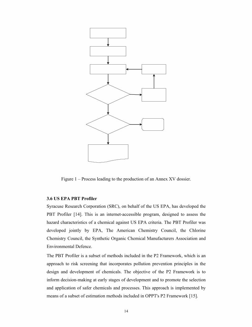
The overall process leading to the Annex XV dossier will normally be started by a

Member State, or the Agency on behalf of the Commission, when they consider that

a substance may be a PBT, vPvB or substance of equivalent concern. The next steps

will be to obtain the relevant available information and review it. If the available

data are considered to be sufficient then the Annex XV dossier can be prepared. In

cases where the data are not considered sufficient in one or more areas, a substance

evaluation should be performed in order to generate the required information. The

information gained through the evaluation will also be reviewed in the same way.

This may be a multi-step process with several iterations. The basic process is set out

in the flow chart of Figure 1.

14

Figure 1 – Process leading to the production of an Annex XV dossier.

3.6 US EPA PBT Profiler

Syracuse Research Corporation (SRC), on behalf of the US EPA, has developed the

PBT Profiler [14]. This is an internet-accessible program, designed to assess the

hazard characteristics of a chemical against US EPA criteria. The PBT Profiler was

developed jointly by EPA, The American Chemistry Council, the Chlorine

Chemistry Council, the Synthetic Organic Chemical Manufacturers Association and

Environmental Defence.

The PBT Profiler is a subset of methods included in the P2 Framework, which is an

approach to risk screening that incorporates pollution prevention principles in the

design and development of chemicals. The objective of the P2 Framework is to

inform decision-making at early stages of development and to promote the selection

and application of safer chemicals and processes. This approach is implemented by

means of a subset of estimation methods included in OPPT's P2 Framework [15].

15

The tool includes methods for estimating environmental persistence (P),

bioconcentration potential (B), and aquatic toxicity (T) built upon SRC’s EPISUITE

software that estimates physico-chemical properties, environmental fate and effects

of molecules using models that are either fragment or Kow based QSARs, or expert

systems, or some combination of the three.

For persistence, the PBT Profiler determines a substance’s half-life in air, water, soil,

and sediment based on the AOPWIN and BlOWIN 3 models and certain

assumptions. The medium (or media) in which a chemical is most likely to be found

is identified by using a Mackay Level III multi-media mass balance model (fugacity

model). This medium is then selected and the model assigns a rank of ‘high’,

‘medium’, or ‘low’ to the chemical by comparing against US EPA criteria.

Bioaccumulation is estimated according to the BCFWIN model. Finally, toxicity is

determined from the chronic value estimated by the QSARs in ECOSAR and, again,

after criteria comparison, the same rankings are applied.

In addition, the PBT Profiler compares results with the PBT criteria established for

Premanufacture Notices (PMNs) submitted under section 5 of TSCA; and the final

rule for reporting chemicals under the Toxic Chemical Release Inventory (TRI).

Results are displayed in three levels of detail, with useful information for

management of any potential risks associated with the chemical.

It is emphasised by the EPA that it does not rely solely on results of screening level

methods, such as the PBT Profiler, to regulate chemicals. The PBT Profiler is used

as a screening level method that provides estimates of PBT characteristics, and is

useful for establishing priorities for chemical evaluation when chemical-specific data

are lacking. If the PBT Profiler identifies an issue of potential concern, additional

data should be gathered and/or additional analyses conducted to come to an informed

decision about the chemicals under review.

3.7 Canadian Domestic Substances List categorisation

Criteria for persistence, bioaccumulation and inherent toxicity (PBiT) are used by

Environment Canada to assess approximately 23,000 substances listed on the

Domestic Substances List (DSL). Criteria for persistence and bioaccumulation are

defined in the Regulations for Persistence and Bioaccumulation [16]. These criteria

were developed from the Toxic Substances Management Policy [17], which provides

16

a common science-based management framework for toxic substances in all

Canadian federal programmes and initiatives. The definition of inherently toxic to

non-human organisms is under consideration by Environment Canada. Those

substances found to be persistent or bioaccumulating and inherently toxic proceed to

the second phase, a screening level risk assessment. Depending on the outcome of

the screening level risk assessment, one of the following outcomes can take place:

• if the screening level risk assessment indicates that the substance does not cause

a risk to the environment or human health, no further action is taken;

• the substance is added to the Priority Substances List to assess more

comprehensively the possible risks associated with the release of the substance;

• it is recommended to add the substance to the list of Toxic Substances in

Schedule I of CEPA (Canadian Environmental Protection Act), if the screening

level risk assessment indicates clear concerns. Substances on Schedule 1 can be

considered for regulatory controls, including, if the substance is not a naturally

occurring substance, virtual elimination.

Under this process, risk assessment principles are applied to priority materials. The

screening assessment is a tiered process, with decreasingly conservative assumptions

as one proceeds up the tiers. An Estimated Exposure Value (EEV) and a Critical

Toxicity Value (CTV) are derived.

In Tier I, the EEV will likely be the highest estimated or measured environmental

concentration available. The CTV, similarly, will be based on toxicity to the most

sensitive organism tested. The CTV is then divided by the necessary assessment

factor(s) to derive the Estimated No Effects Value (ENEV). A Tier 1 quotient is

calculated by dividing the EEV by the ENEV. If the result is less than 1, the

substance is considered not to be ‘toxic’ under CEPA for the assessment endpoint

and no further assessment is needed. If it is greater than 1, then the substance is

assessed further, using less conservative (more data intensive) assumptions (Tiers II

or III). If a substance ‘fails’ in Tier III (EEV/ENEV > 1), then it is considered to be

CEPA toxic and put on Schedule 1.

17

3.8 PBT Japanese chemical legislation

The ‘Chemical Substances Control Law’ ratified in 1973 [18] aims at preventing

damage to human health caused by environmental pollution from chemical

substances. According to the latest amendment to the Chemical Substance Control

Law of 1st April 2004 new chemical substances undergo a volume-dependent

ecotoxicological and toxicological testing scheme by the notifier before approval for

manufacture/supply to the Japanese market. In addition, under the Existing

Chemicals Programme sponsored by the Japanese Government, existing substances

which are not covered by the legislation for new chemicals also undergo systematic

testing.

Hazard endpoints, such as persistence in combination with ecotoxicity or long-term

toxicity or confirmed potential for damage by environmental pollution, can lead to

specific classification and regulation of chemical substances. In addition, substances

identified as exhibiting persistence and bioaccumulative properties can be placed

under legal control by classification as Type I Monitoring Substances or ultimately

as Class I Specified Chemical Substances. Currently 13 substances have been

designated as Class I specified Chemical Substances. Regulatory measures for Type

I Monitoring Substances comprise mandatory reporting of quantities of manufacture,

import and use, risk reduction measures according to a preliminary toxicological

evaluation by the authorities and the requirement for further investigation of long-

term ecotoxicity/toxicity. Class I Specified Chemical Substances are banned from

production and import unless they are specifically approved for use by the

authorities.

18

4. OVERVIEW OF PBT AND vPvB CRITERIA

National, regional and international bodies are developing ways to manage PBT and

POP chemicals to better protect human health and the environment. At present there

is little coordination or consistency between the approaches and the criteria defined

by different authorities to select and manage PBT substances.

The OSPAR Convention for the Protection of the Marine Environment of the North-

East Atlantic on the Marine Environment aims to prevent pollution by continuously

reducing discharges, emissions and losses of hazardous substances (identified by

specific PBT criteria), with the ultimate aim of achieving concentrations in the

marine environment near background values for naturally-occurring substances or

close to zero for man-made substances.

The European Union REACH regulation under discussion considers PBT chemicals

as substances of particular concern due to the uncertainty of predicting exposures

and concentrations that cause unwanted effects. As such, the EU is proposing the use

of specific criteria to identify PBT substances, and very persistent and very

bioaccumulating substances (vPvBs). For this second category, the EU says it is not

necessary to demonstrate toxicity as long-term effects can be anticipated.

The Environmental Protection Agency (USA) has proposed two sets of criteria for

PBTs under the Toxic Substances Control Act. These define substances that will

have to be controlled and others that will have to be banned.

The Canadian Government is also developing PBT criteria in the context of its Toxic

Substances Management Policy. The assessment of persistence and bioaccumulation

properties for new substances notified in Canada relies on the criteria listed in the

Persistence and Bioaccumulation Regulations [16]. The inherent toxicity (iT) of a

new substance is determined and used in the risk assessment. Currently,

Environment Canada is examining policy to address new substances that are PBiT,

separately from conclusions of the risk assessment. New substances that are assessed

as P and B and found “suspected of being Canadian Environmental Protection Act

(CEPA)-toxic”, that is, found to be of risk to the environment, are subject to the

19

virtual elimination policy described under the Toxic Substances Management Policy

(TSMP) [17].

The OECD conducted a survey of approaches in the assessment of new chemicals in

different countries, in preparation for an OECD Workshop on new chemicals

notification and assessment in 2002. This survey showed that, as in the US, Austria

had recently developed criteria for PBT substances that reflected levels of concern.

New chemicals with PBT properties may be judged persistent and bioaccumulating

or very Persistent and very Bioaccumulating (vPvB). As in Canada and the US the P

and vP criteria are half-lives in the various environmental compartments. In some

other nations, notably Japan and the United Kingdom, there was no formal

recognition of PBT substances as a category; nevertheless new chemical notification

dossiers were reviewed for the core PBT characteristics of persistence,

bioaccumulation and toxicity. The main PBT criteria are illustrated in Table 1.

20

Persistence Bio-accumulation Toxicity

OSPAR PBT criteria

Not readily biodegradable or half-life in water > 50 days

LogKow > 4 Or BCF ≥ 500

Acute aquatic toxicity L(E)C50 £ 1 mg/l or long term NOEC £ 0.1 mg/l or mammalian toxicity: CMR1 chronic toxicity

EU PBT criteria

Half-life > 60 days in marine water, or > 40 days in fresh- or estuarine water, or > 180 days in marine sediment, or > 120 days in fresh- or estuarine water sediment is higher, or > 120 days in soil

BCF > 2000

Chronic NOEC< 0.01 mg/l for marine or freshwater organisms, or the substance is classified as carcinogenic (cat. 1 or 2), mutagenic (cat. 1 or 2), or toxic for reproduction (cat. 1, 2, or 3).

EU vPvB criteria

Half-life > 60 days in marine, fresh or estuarine water, or > 180 days in marine, fresh or estuarine water sediment, or > 180 days in soil

BCF > 5000 Not applicable

US EPA Control action2

Transformation half-life > 2 months

BCF > 1000 Toxicity data based on level on risk concern

US EPA Ban Pending3

Transformation half-life > 6 months

BCF ≥ 5000 Toxicity data based on level on risk concern

Canada Toxic Substance Management Program (TSMP)4

Half life in Air > 2 days Water > 2 months Sediment > 6 months Soil > 1 year

BAF or BCF > 5000 or LogKow > 5

Inherently toxic

Table 1 - PBT criteria. 1CMR - carcinogenic, mutagenic or toxic to reproduction. 2Testing and release control required. 3Commercialisation denied except if testing

21

justifies removing chemical from “high risk concern”. 4The Canadian Domestic Substances List uses different criteria (water>6 months, sediment>1year, soil>6 months) to define substances which will undergo full elimination (P and B and T and predominantly anthropogenic) and those which will undergo in-depth risk assessment (P or B and T and predominantly anthropogenic).

4.1. REACH PBT criteria

A substance that fulfils all three of the criteria below is a PBT substance.

Persistence

A substance fulfils the persistence (P-) criterion when:

the half-life in marine water is higher than 60 days, or

the half-life in fresh- or estuarine water is higher than 40 days, or

the half-life in marine sediment is higher than 180 days, or

the half-life in fresh- or estuarine water sediment is higher than 120 days, or

the half-life in soil is higher than 120 days.

The assessment of the persistency in the environment should be based on available

half-life data collected under the adequate environmental conditions which should be

described by the registrant.

Bioaccumulation

A substance fulfils the bioaccumulation (B-) criterion when:

the bioconcentration factor (BCF) is higher than 2000.

The assessment of bioaccumulation should be based on measured data on

bioconcentration in aquatic species. Data from freshwater as well as marine water

species can be used.

Toxicity

A substance fulfils the toxicity (T-) criterion when:

the long-term no-observed effect concentration (NOEC) for marine or

freshwater organisms is less than 0.01 mg/l, or

the substance is classified as carcinogenic (category 1 or 2), mutagenic

(category 1 or 2), or toxic for reproduction (category 1, 2, or 3), or

22

there is other evidence of chronic toxicity, as identified by the classifications:

T, R48, or Xn, R48 according to Directive 67/548/EEC.

4.2. REACH vPvB criteria

A substance that fulfils the criteria below is a vPvB substance.

Persistence

A substance fulfils the very persistence criterion (vP) when:

the half-life in marine, fresh- or estuarine water is higher than 60 days, or

the half-life in marine, fresh or estuarine water sediment is higher than 180

days, or

the half-life in soil is higher than 180.

Bioaccumulation

A substance fulfils the very bioaccumulative criterion (vB) when:

the bioconcentration factor is greater than 5000.

In order for a substance to be designated a PBT or a vPvB substance, all of the

relevant criteria have to be demonstrated to be fulfilled for the substance.

23

5. METHODS FOR PBT DATA GENERATION

For most substances the available data do not enable to decide with certainty whether

the substance should be considered under the PBT assessment or not. This motivates

the need to use screening data that identify whether the substance has the potential to

be a PBT/vPvB.

In deciding which information is requested (on P, B or T) special care should be

taken to avoid animal testing wherever possible. This implies that when for several

properties further information is needed the assessment should be focused on

clarifying the potential for persistence first. When it is clear that the P criterion is

fulfilled, a stepwise approach should be followed to elucidate the B criterion,

eventually followed by toxicity testing to clarify the T criterion. However, it is

recognised that it may sometimes be more convenient to start the PBT assessment by

evaluating the B criterion.

5.1 Persistence data generation

The persistence of a substance reflects the potential for long-term exposure of

organisms but also the potential for the substance to reach the marine environment

and to be transported to remote areas. The assessment of the potential for persistency

in the marine environment should in principle be based on actual half-life data

determined under marine environmental conditions. When these key data are not

available other types of available information on the degradability of a substance can

be used to decide if further testing is needed to assess the potential persistence. In

this approach three different levels of information are defined according to their

perceived relevance to the criteria:

experimental data on persistence in the marine environment;

other experimental data;

data from biodegradation estimation models.

This approach reflects existing knowledge on biodegradation and is considered a

pragmatic approach to make optimal use of the available data and methods. Research

is ongoing to better estimate the persistence in the marine environment from existing

biodegradation tests. Moreover, other degradation mechanisms such as hydrolysis

and photolysis should be taken into account where they can be shown to be relevant.

24

In principle the persistence in the marine environment should be assessed in

simulation test systems that determine the half-life under relevant environmental

conditions. The determination of the half-life should include assessment of

metabolites with PBT characteristics. The half-life should be used as the first and

main criterion in order to determine whether a substance should be regarded as

persistent. Hence appropriate half-life data from valid simulation tests override data

from the other levels of information.

Tests performed under marine conditions should use media from marine areas not

directly influenced by freshwater outlets or runoffs. It is not possible to establish

specific criteria and each test must be evaluated case-by-case. However, the content

of freshwater in the sample should be low (i.e. a large dilution as determined, for

example, by salinity), the sample should be taken from the water column (and not the

surface), the content of microorganisms should be low (compared to freshwater) and

cross-contamination during handling, transport and testing should be avoided.

In case no half-life data are available for marine water or sediment the decision

whether a substance is potentially persistent needs to be based on other experimental

data. If available, use can be made of the half-life values from simulation tests of

degradation in freshwater. Extrapolation of the existing biodegradation information

(either measured data from ready and inherent tests or results from QSAR

modelling) to degradation rates in the marine environment is very difficult and care

should be taken not to over-interpret the outcome of such tests. However, in order to

use the available information to select potentially persistent substances, this

information should be used.

For new substances, priority existing substances and biocides, information from a

ready biodegradability test is normally available and therefore an initial decision

whether the substance is potentially persistent can be taken. However, for many

other substances no data will be available or the available information is difficult to

interpret. For these substances it can be helpful to apply models that estimate the

potential for biodegradation in the environment.

In a preliminary assessment whether a substance has a potential for persistence in the

marine environment and hence for asking for actual test data the use of the BIOWIN

program is proposed [19]. This program estimates aerobic biodegradability of

organic chemicals using six different models (linear, non-linear model, ultimate and

25

primary biodegradability timeframe model, MITI linear and non-linear model). The

use of the results of these programs in a conservative way may fulfil the needs for

evaluating the potential for persistency. The use of three out of the six models is

suggested as follows:

non-linear model prediction: does not biodegrade fast (<0.5) or

MITI non-linear model prediction: not readily degradable (<0.5) and

ultimate biodegradation timeframe prediction: > months (<2.2)

When predictions of these three models are combined most not readily

biodegradable substances will be identified, without at the same time causing a

significant increase in the number of falsely included readily biodegradable

substances.

The preliminary character of this method to identify potentially persistent substances

in the marine environment is emphasised, and further possible development of a

suitable methodology is recommended.

5.1.1 Biodegradation data

Biodegradation data are highly dependent on the substrate’s chemical structure and

initial concentration. The activity of the degrading microbial population is also

equally important to how and whether a substance is biodegraded. It is determined

by the species initially present in the inoculum, their relative population densities,

the induction of their enzymes, and their ability to grow once exposed to a chemical.

Environmental conditions, such as temperature, salinity, pH, oxygen concentration

(whether aerobic or anaerobic), redox potential, concentration and nature of various

substrates and nutrients, concentration of heavy metals (which may be toxic), and

effects (synergistic and antagonistic) of associated micro-flora also have a major

effect on biodegradation rates through their effects on microbial activity [20].

Biodegradation results are often highly dependent upon the test protocol. Many

screening tests (such as the stringent ready biodegradability tests) do not employ an

acclimation step prior to starting the test and/or may not be run long enough to allow

for acclimation during the test. Therefore, the chemical may not start to biodegrade

in the normal 28 day allowed for in most screening biodegradation tests. Futhermore,

it is generally needed for the indirect analytical methods, to keep the concentration of

26

the test chemical higher than what is usually found in the environment; as a

consequence, some chemicals toxic chemicals may result in no biodegradation, but

not because they are nonbiodegradable. The effects of test variables on the

biodegradation rates have been reviewed by Howard in 2000 [21]. In addition, the

reproducibility of individual tests is often poor, especially between laboratories, and

in some cases even within the same laboratory. Test guidelines developed by the

Organization for Economic Cooperation and Development ([OECD], Paris, France)

and the U.S. EPA’s Office of Pollution Prevention and Toxics and Office of

Pesticide Programs, together with analytical methods and criteria for whether a

chemical is considered to be biodegradable (pass) or nonbiodegradable (fail), have

been summarized by Howard [21]

One of the most important screening tests is the MITI-I test, also known as OECD

301C. The MITI-I is a screening test in which the test substance is initially present at

100 mg/L and the inoculum is 30 mg sludge solids/L. The test measures BOD and,

like other OECD ready biodegradability tests, normally last for 28 days. If oxygen

demand due to degradation of test substance reaches or exceeds 60% of theoretical,

the test substance is considered readily biodegradable. The MITI inoculum is

prepared using a process of feeding a mixture of sludges from various sources for 30

days with peptone only. This standardization reduces the diversity of micro

organisms in the sludge and also their ability to acclimate to and degrade various

substrates. Apparently this reduces variability in the results and thereby makes the

test of higher utility.

5.2 Bioaccumulation data generation

In the regulatory context, the assessment of the (potential for) bioaccumulation in the

context of the PBT assessment makes use of measured bioconcentration factors in

marine or freshwater organisms. It is important to recognise that the concentration in

the aqueous phase must be that in the free solution (i.e., not including that sorbed on

to organic matter in the water or on to the surface of the test vessel). In general, for

chemicals that are not highly hydrophobic (LogKow < 5). the total aqueous

concentration can be taken as equal to the freely dissolved concentration. However,

for very hydrophobic chemicals this may not be the case [22].

27

In Europe, the U.S., and Canada a flowthrough method [23] is used in which two

groups of organisms of the species under investigation are exposed to water and a

constant concentration of the test chemical, respectively, until steady state is

achieved or for at least 28 to30 days: this is followed by an elimination phase in

which they are exposed to water only for a period of about twice the uptake period.

During the tests, organisms and water are removed in geometric time series and

analysed. From these data the uptake and elimination rate are calculated, and the

ratio of the two gives the BCF.

Several guidelines for the experimental determination of bioconcentration are

available. The OECD monograph [24] describes static, semistatic, and flow-through

methods; Gobas and Zhang [25] developed a method suitable for very hydrophobic

chemicals.

The great variability in measured BCF values for a given chemical was highlighted

by Nendza [26]. She identified a number of factors that contribute to such variability

including test species; the size, age, and sex of the test species; purity of the test

chemical; lipid content fish; whether or not steady state is reached during the test;

analytical method used; stability of the test chemical in water; presence of

surfactants; pH and buffer capacity; water chemistry (hardness), co-solute effects;

and presence of suspended organic matter. In general, experimental measurement of

bioconcentration is time-consuming and expensive. To measure BCF values for the

large number of chemicals that are of potential regulatory concern is not feasible. For

this reason attention is turning to estimation of BCF values by QSARs. QSAR

models for bioconcentration have been recently reviewed by the ECB [27].

In addition to the above-mentioned data on bioconcentration or bioaccumulation in

aquatic species, evidence that a substance shows high bioaccumulation in other

species may also be used to decide whether the B criterion is fulfilled. Such evidence

may be based on information from specific laboratory tests or from field studies.

Specific attention needs to be paid to measured data in biota. Measured data in biota

are a clear indicator that a substance is taken up by an organism. However, they are

not an indicator that significant bioconcentration or bioaccumulation has occurred.

The interpretation of such data in terms of actual bioaccumulation or

biomagnification factors can be especially difficult when the sources and levels of

28

the exposure (through water as well as through food) are not known or cannot be

estimated reasonably.

5.3 Toxicity data generation

For persistent and bioaccumulative substances, long-term exposure can be

anticipated and expected to cover the whole life-time of an organism and even

multiple generations. Therefore chronic or long-term ecotoxicity data, ideally

covering the reproductive stages should in principle be used for the assessment of the

T criterion. In practice, however, the principal data available for most chemicals will

be for short-term effects, and this must, in the first instance, be used to drive initial

selection. Mammalian toxicity data must also be considered in the selection due to

the fact that toxic effects on top predators, including man, may occur through long-

term exposure via the food-chain.

Where data on chronic effects are not available, short-term toxicity data for marine

or freshwater organisms can be used to determine whether a substance is a potential

PBT provided the screening criteria for P and B are fulfilled. In the context of the

PBT assessment a substance is considered to be potentially toxic when the L(E)C50

to aquatic organisms is less than 0.1 mg/l. If a substance is confirmed to fulfil the

ultimate P and B criteria chronic toxicity data are required to deselect this substance

from being considered as a PBT. In principle chronic toxicity data, when obtained

for the same species, should override the results from the acute tests.

In case where no acute or chronic toxicity data are available the assessment of the T

criterion at a screening level can be performed using data obtained from QSARs.

29

6. BIODEGRADATION DATABASES

Nowadays various biodegradation databases are suitable for a direct evaluation and

development of qualitative models or classification rules. When assessing data

derived from these databases it is important that the quality of the data be confirmed.

Some databases are publicly available, e.g. Syracuse BIODEG. When reporting the

use of such databases, it is important that the version of the database used is

mentioned. The most widely used databases are described below.

6.1 BIODEG Database

The BIODEG database was developed through the collaborative efforts of the EPA's

Office of Toxic Substances and the Syracuse Research Corporation (SRC) [28], [29].

It contains “high-quality” biodegradation data for about 300 diverse commercial

chemicals. A substance is included in the database only if it had two or more

biodegradability studies with consistent results; if a clear judgement of slow or fast

biodegradation could be made; and if the data indicated that acclimation would not

play a major role. This database, available at http://www.syrres.com/esc/biodeg.htm,

includes over 6,600 records with information about the biodegradation of 815

chemical substances in several types of experiments (biological treatment

simulations, screening tests, field studies, grab sample tests, etc.) under a variety of

experimental conditions (e.g., aerobic, anaerobic, etc).

6.2 BIOLOG Database

The BIOLOG database was also developed through the collaborative efforts of

EPA's Office of Toxic Substances and the Syracuse Research Corporation (SRC). It

is an index of published literature on the biodegradation and microbial toxicity of

chemical substances. Over 62,600 records cover more than 7,850 different

chemicals. The database available at http://www.syrres.com/esc/biolog.htm covers

both biodegradation and toxicity of substances to microbial populations. BIOLOG

can be used as a standalone database or in conjunction with other substance-oriented

databases already available through CIS (such as AQUIRE, ENVIROFATE, the

MERCK INDEX Online, and RTECS). CIS is operated by the Oxford Molecular

30

Group, Inc. It is an online information service that offers access to more than 30

databases dealing with chemistry, hazardous materials, toxicology, and

environmental issues.

6.3 MITI Database

The largest available biodegradation database contains the so-called MITI-I test data

[30], [31], [32] which comprises results of a single uniform biodegradation test for

nearly 900 commercial chemicals. The MITI-I test is a screening test for “ready”

biodegradability in an aerobic aqueous medium and is described in OECD [33]-[34]

and EU [35] test guidelines. The MITI-I test was developed in Japan, and it now

constitutes one of the six standardised “ready” biodegradability tests described by

EU and OECD regulations. For the MITI-I test, 100 mg/L of test substance is

inoculated and incubated with 30 mg/L sludge. Biological oxygen demand (BOD) is

measured continuously during the 28-day test period. The pass level for “ready”

biodegradability is reached, if the BOD amounts to ≥60% of theoretical oxygen

demand (ThOD). Biodegradation data determined according to the MITI-I test

protocol are now available for 894 substances of diverse chemical structures. The

majority of data has been published [36], and a smaller fraction has been obtained

through the Japanese Existing Chemicals Law program directed by the MITI [30].

6.4 ESIS Database

The European chemical Substances Information System (ESIS) is an IT System

which provides information on chemicals related to EINECS (European Inventory of

Existing Commercial chemical Substances), ELINCS (European List of Notified

Chemical Substances), NLP (No-Longer Polymers), HPVCs (High Production

Volume Chemicals) and LPVCs (Low Production Volume Chemicals), including EU

Producers/Importers lists, C&L (Classification and Labelling), Risk and Safety

Phrases, IUCLID Chemical Data, Priority Lists, and a tracking system for risk

assessments conducted according to Existing Substances Regulation (ESR), i.e.

Council Regulation (EEC) 793/93.

ESIS includes more than 2600 records. Chemicals can be searched by chemical

name, CAS number, and molecular formula. The use of the on-line database is free

and can be accessed via the Internet (http://ecb.jrc.it/esis). All relevant information

31

on species, chemicals, test methods and test results are abstracted. The data are

available for downloading as pdf files.

6.5 University of Minnesota Biocatalysis/Biodegradation Database (UM-BBD)

This database contains information on microbial biocatalytic reactions and

biodegradation pathways for primarily xenobiotic, chemical compounds [37]. The

goal of the UM-BBD is to provide information on microbial enzyme-catalyzed

reactions that are important for biotechnology. The reactions covered are studied for

basic understanding of nature, biocatalysis leading to specialty chemical

manufacture, and biodegradation of environmental pollutants. Individual reactions

and metabolic pathways are presented with information on the starting and

intermediate chemical compounds, the organisms that transform the compounds, the

enzymes, and the genes. In addition to reactions and pathways, this database also

contains Biochemical Periodic Tables and a Pathway Prediction System. The

database is available at http://umbbd.msi.umn.edu/index.html.

6.6 California Department of Food and Agriculture Biodegradation Database

A small source of biodegradation rates for pesticides is developed by the California

Department of Food and Agriculture. The database comprises aerobic and anaerobic

soil metabolism half-lives based on published scientific literature as well as studies

submitted to the California Department of Food and Agriculture by chemical

companies as a consequence of the “data-call-in” requirements of the Pesticide

Contamination prevention Act. These values have been reproduced in Howard [1]

In addition to these online databases, biodegradation data have been collected in a

number of books [38]-[39].

32

7. QSARS FOR BIODEGRADATION

New laws resulting from enactment of the United Nations Stockholm Convention in

May 2004 together with the new REACH legislation, have led to significant new

activity in the assessment of Persistent, Bioaccumulative, Toxic substances (PBT).

The categorisation of thousands of commercial substances is needed and it is

estimated that screening level assessments for the categorised chemicals will require

a significant effort and conducting biodegradation tests would be expensive and time

demanding.

The limited empirical persistence, bioaccumulation and toxicity data, the high test

costs together with the regulatory constraints and the international push for reduced

animal testing motivates a greater reliance on QSAR models in the PBT assessment.

Several evaluation studies have been performed on biodegradation models, including

qualitative as well as (semi) quantitative models. However, the development of

Quantitative Structure-Biodegradation Relationships (QSBRs) has been relatively

slow compared with proliferation of QSARs, especially for toxicity endpoints

because of the nature of the biodegradability endpoint. Biodegradation is a complex

process consisting of many steps that critically depend on chemical structure,

environmental conditions into which a chemical is released and the bioavailability of

the chemical. In addition, results of the biodegradation tests are strongly influenced

by the physicochemical properties of chemical such as solubility, toxicity, test

concentration. Therefore, experimental biodegradation data are highly variable.

An evaluation study has been performed within the EU project “QSAR for

Predicting the Fate and Effects of Chemicals in the Environment” [40]-[42]. This

evaluation study showed that 200 models had been published for various degradation

processes in air, soil, and water systems by the first quarter of 1994.

The earliest QSBRs developed in the 80s were statistical correlations between

biodegradability endpoint and physical-chemical properties [43] or molecular

descriptors [44]. This was the approach directly reapplied from toxicity modelling.

The earliest studies focused on class-specific models (QSBRs), because significant

and mechanistically reasonable correlations between biodegradability and molecular

33

structure could be established only within congeneric series of chemicals [45]

because the descriptors used could not well describe individual fragment

contributions but rather integrated properties of the whole molecule. However, the

mere existence of a series of chemicals that are apparently congeneric does not

guarantee that they always biodegrade by a common mechanism or pathway,

however chemically similar they appear to be.

Several QSAR biodegradation models have been developed for selected groups of

structurally similar compounds [46]. For example, models have been developed to

predict the biodegradation of a limited number of alcohols [47], n-alkyl phthalates

[48], chlorophenols and chloroanisoles [49], para-substituted phenols [50], and

meta-substituted anilines [51].

The vast majority of these QSBRs rely on the octanol/water partition coefficients,

van der Waals radii, alkaline hydrolysis rate constants and molecular connectivity

indices. Generally the correlation between physicochemical properties or molecular

descriptors and biodegradation rates were good, but overall these models have not

been used much. Their applicability is limited to the specific classes for which these

models were developed, and it is inappropriate to predict biodegradation rates for

chemicals outside of those classes.

The major obstacle that precluded the development of better and reliable

biodegradation models in the past was the absence of standardised and uniform

biodegradation databases. Several years ago, two databases of “high-quality”

biodegradation data became generally available, i.e., the BIODEG database Syracuse

Research Corporation of evaluated and standardised biodegradation data and the

MITI database containing the results of a single screening test for “ready”

biodegradability in aerobic aqueous medium (see Chapter 6).

Consequently, recent years have been characterised by a very intensive development

of new and better qualitative and quantitative biodegradability models by the

application of new and advanced computational and statistical methods.

In an OECD report, 78 different SARs for biodegradation were presented and

validated with more than 700 experimental data [52]. In addition, a literature search

on SARs for biodegradation was performed including literature published until 1994

[53], [54]. In this study, 84 models were evaluated. The main conclusion in both

studies was that only a few models provided an acceptable level of agreement

34

between estimated and experimental data. According to the mentioned studies, the

group contribution method developed to generalise the applicability of QSBRs to

large and structurally diverse sets of chemicals seems to be the most applied and

successful way of modelling biodegradation. These models are based on a direct link

between molecular structure and biodegradability expressed as a function of the

contribution of each fragment encountered in the molecule and therefore have the

possibility of straightforward interpretation. On the assumption that molecular

fragments may have an enhancing or retarding effect on biodegradability, weighted

molecular fragments are used as model descriptors.

To determine the fragment contribution weights, each molecule from a training set is

decomposed into fragments that are assigned weights, and its biodegradability is

assessed based on the weights of the fragments. Various statistical techniques have

been used in determining weights: linear [55], [56] and non-linear regression

modelling [57] partial least square (PLS) [30] and neural networks [58]. The

endpoints modelled were semi-qualitative rates distinguishing among days, weeks,

months [55]-[57] or Boolean (yes/no) determination of ready biodegradability [30].

While the group contribution approach allows structurally diverse sets of chemicals

to be analysed it has the disadvantage of being dependent on the type and number of

a priori selected fragments. Thus, the results of QSBR studies are strongly affected

by the way the molecule is fragmented. To avoid this, the MultiCASE approach [59]

has been developed to generate all possible fragments of the molecules and to

subsequently select the statistically most significant ones to the endpoint of interest.

These fragements are then used to establish regression models between screened

fragments and the endpoint. In MultiCASE terminology, fragments associated with

biodegradability are termed biophores, whereas fragments associated with resistance

to degradation are termed biophobes. The novelty added to the fragment-based

biodegradation model by MultiCASE is that the fragment selection is performed

based on the data set instead of predefined by empirical rules or extracted from

fragment databases. MultiCASE offers greater flexibility than ordinary least-squares

regression models because, as with neural networks and, to some degree with

modern regression methods (PLS, genetic algorithm-variable subset selection), the

structure of the model is not defined a priori.

35

The predictive ability of fragment contribution methods has been evaluated recently

and reaches 72-80% for ready biodegradable chemicals and ca. 80-85% for non-

ready biodegradable chemicals [60]. Consistently, the method has been found to

perform well in predicting not ready biodegradable chemicals but somewhat less

effective in the prediction of ready chemicals. This is attributed to the approach

because the analyses are limited to fragments in the parent structures and not of those

in the metabolites and therefore are likely to overestimate the relative weights of

fragments that are difficult to biodegrade.

MultiCASE model results are relatively easy to understand, and mechanistic

interpretations can be developed, although this process is not always straightforward.

However it might be affected by some potential problems highlighted in Jaworska et

al. [61]. One potential drawback is that since biodegradation databases tend to be big

but with large molecular complexity, the possibility exists for overfitting the data.

Another potential disadvantage is that, since biophores and biophobes are developed

from training sets individually, important structural influences on biodegradability

may or may not be represented in any given training set. Thus, as with other

fragment-based methods, a key fragment or fragment interaction may be missed and

the model may fail when extended to chemicals outside that training set.

Another approach is based on chemometric methods for biodegradability prediction

[62]. Both regression and classification models have been developed. Regression

models are usually based on ordinary least squares, but sometimes logistic regression

is used as well. Classification methods are quantitative models using selected

molecular descriptors for the prediction of a qualitative property, such as the

partition of a set of compounds into different predefined classes (e.g., readily

biodegradable/not readily biodegradable). Both types of model are based on

statistically selected sets of relevant descriptors, and attention is devoted mainly to

the prediction power of the models. Genetic algorithms (GA) and simulated

annealing are techniques often used in chemometric analysis to search for the most

predictive descriptors, in the so-called variable subset selection process [63], [64].

These approaches, based on large sets of molecular descriptors, do not require any a

priori assumptions regarding model structure. The reason for the GA’s selection of

specific descriptors in the modelling and prediction is not always readily

36

interpretable. The descriptors selected by GAs as the best combinations correlated to

a response are not necessarily the best for understanding the mechanism. Their

practical value relies on their predictive ability in the model, which should be

carefully tested by validation techniques (e.g. cross-validation, bootstrapping,

scrambling of response, prediction reliability.).

The opinion that there is a need to involve pathway information for modelling

biodegradability of chemicals initiated the development of the third class of QSBR

studies based on expert systems that represent artificial intelligence approaches

[65]. These models simulate biodegradation pathways based on transformation rules

from the data. The so-called knowledge-based expert systems act as a collection of

expert knowledge about phenomena or a process that, like biodegradation, can be

described by a set of rules. The library of rules or transformations is organised in a

hierarchy that orders the rules by their likelihood of being executed. Since they are

aimed to predict biodegradation pathways, these models claimed to be based on a

mechanistic approach. Generally expert systems are qualitative in nature, but they

can be linked to other models to provide a quantitative assessment. The most

important component of an expert system that simulates biodegradation pathways is

the hierarchy of rules. Even if the rules are correct, if the hierarchy is not set

correctly, the system will not suggest the correct biodegradation process. While in

knowledge-based expert systems, the rules and hierarchy are manually established

by a group of experts, in the case of the so-called inductive or machine-learning

expert systems, the rules and hierarchy are developed without human input. Through

examination of the data, the computer deduces sets of rules that best describe the

modelled endpoint. This approach is less intuitive than the knowledge-based

approach and may lead to predicted transformations that are not likely in nature.

However, machine-learning systems could lead to the identification of new rules, not

previously known to experts, and is not affected by the arbitrariness intrinsic in the

knowledge-based expert systems. The inductive learning expert systems are often

built with GA and when applied to biodegradation modelling are limited to parent

compound analysis, without considering intermediate steps in a pathway..

The expert systems approach was first implemented in one of the META [66]

automatic rule induction programs that predicts qualitatively the aerobic

37

biodegradation pathway [67]. It has 70 general transformations that were developed

by evaluating MultiCASE biophores in the dictionary. The hierarchy is based on

weights of fragments of the source chemical calculated by MCASE and assigning the

same weights to associated fragment transformations. The hierarchy has been

optimised by using a genetic algorithm [68].

Another approach relying on pathway prediction is the one incorporated in

CATABOL [69], [70]. This is an expert system predicting the biotransformation

pathway working together with a probabilistic model that calculates probabilities of

the individual transformations. The expert system contains a library of hierarchically

ordered individual transformations and a matching substructure engine. The

hierarchy in the expert system is set according to the descending order of the

individual transformation probabilities. The integrated principal catabolic steps are

derived from set of metabolic pathways predicted for each chemical from the

training set and encompass more than one real biodegradation step to improve the

speed of predictions.

In the next sections of this report some of the widest used and most interesting

QSBRs models are presented in more detail, based on a comparative evaluation of

model performance by Rorije et al. [60], the review of broadly applicable methods

for predicting biodegradation by Jaworska et al.[61], and a recent review by Nendza

[71].

7.1 Group contribution approaches

7.1.1 Degner et al. OECD hierarchical model approach

A hierarchical model approach was proposed by Degner et al. [72] for the OECD to

guide the selection of the appropriate biodegradation model based on structural

fragments. The basic principle of the hierarchical model approach is that a set of

discriminant criteria can be used to identify the most suitable model for a given

compound.

The models are Multiple Linear Regression (MLR) models based on structural

fragments to describe ready/not-ready biodegradability. The models are limited to

38

specific classes of chemicals, and trained with the qualitative outcome of the MITI-I

test (ready/not-ready). First the compounds are categorised based on their structural

characteristics, according to their parent structure as well as substructures, in order to

group compounds with a similar degradation pattern. Within the classes defined, the

biodegradation is then be related to same structural descriptors. For acyclic

compounds and mono-aromatic compounds several substructure-based QSARs were

developed.

The two most successful models (for acyclic aliphatic compounds and for

monocyclic aromatic compounds) were validated using the same set of 488 MITI-I

data as for the BIODEG model [55]. They revealed a better performance, especially

for the prediction of ready biodegradation. For acyclic compounds, 93.7% of the

predictions for the ready biodegradable compounds and 80.9% for not ready

biodegradable compounds were correct. For mono-aromatic compounds, 75% of the

predictions for the ready biodegradable, and 90.9% of the predictions for the not

ready biodegradable, compounds were correct. It was noted by Rorije et al. [60] that

these percentages are difficult to compare to the BIODEG model (or any other

general model) since the chance of finding a ready biodegradable compound in the

subset of acyclics is a lot higher than 50% (in this case 81.6%). The same comment

is valid for the chance of finding a not-ready biodegradable compound for mono-

aromatic compounds.

7.1.2 Multivariate Partial Least Squares (PLS) model

A Multivariate Partial Least Squares (PLS) model for the prediction of compounds

that are readily biodegradable was proposed in 1999 by Loonen et al. [73]. The

model is based on 894 substances of widely varying chemical structures with

biodegradation assessed according to MITI-I test protocol (388 readily, 506 not-

readily biodegradable). The chemicals were characterised by a set of 127 structural

fragments defined by Eakin et al. [74]. The model was developed by PLS

discriminant analysis. The PLS model for biodegradation generates predictions on a

continuous scale. Thus, to compare the predictions with the original binary data for

biodegradability, the continuous scale is divided into two areas, >0.55 and <0.45,

corresponding to readily biodegradable and not-readily biodegradable chemicals,

39

respectively. Estimated values between 0.45 and 0.55 are considered as borderline

cases and preferably should not be used.

The examination of the full dataset of 127 fragments indicated that 44 fragments

have positively signed PLS regression coefficients, and thus have an enhancing

effect on the biodegradability of a chemical. The two most important positively

signed fragments are long non-branched alkyl chains. These results conform to the

generally known mechanism of biodegradation; in fact these structures are generally

known to be susceptible to oxidation, resulting in the formation of carboxylic acids,

via primary n-alkyl alcohols and aldehydes. Other fragments associated with a

significant positive effect on the structure’s biodegradability are the presence of one

or more hydroxyl group(s) attached to a chain structure, and one or more carbonyl,

ester, or acid groups attached to either a chain or ring structure. Chain structures with

these fragments are susceptible to common oxidation processes that involve the

formation of carboxylic acids through the intermediate formation of aldehydes. The

aromatic ring structures with these fragments degrade through the formation of

catechol followed by ring opening.

The remaining 83 fragments were associated with negatively signed regression

coefficients, indicating that they have a retarding effect on biodegradability. The

most important fragments with a retarding effect on biodegradability are fragments

indicating the presence of one or more aromatic rings, and fragments related to the

presence of one or more halogen substituents on either a chain or ring structure.

Again, these findings are consistent with observations that aerobic biodegradation

decreases with increasing degree of halogenation.

The model has been evaluated by internal cross validation and repeated external

validations. It showed very good classification ability, with about 85% of the model

predictions being correct for the complete dataset. The model predicts slightly better

(86%) the “not-ready” compounds than the “ready” compounds (84%). The averaged

percentage of correct predictions from four external validation studies was 83%.

However, no predictions were made for about 10% of all chemicals because their

estimated values were between 0.45 and 0.55. As described earlier, this is the

borderline area between readily biodegradable or not-readily biodegradable

substances, and those estimates are not reliable and should not be used. The

40

influence of interactions between fragments within the same molecule was also

investigated.

Model optimisation by a two-step variable selection was performed with fragment–

fragment interactions to keep the model size manageable. For the variable selection,

only 97 fragments that were present in at least five substances were included. The

most important fragment–fragment interactions were then selected on the basis of

their PLS regression coefficients. With these additional fragment-fragment

interactions (706), the model classification ability increased to 89% overall. The

improved classification ability with the addition of fragment–fragment interaction

variables is almost entirely related to the “not ready” biodegradable substances since

their predictions increased from 86% to 92%.

7.1.3 Biodegradation Probability Program BIOWIN

The Biodegradation Probability Program (BIOWIN) [55],[57],[29] estimates the

probability of rapid aerobic biodegradation of an organic chemical in the presence of

mixed populations of environmental microorganisms.

The original model was developed by linear and non linear regression based on 35

structural fragments using a database of weight-of-evidence evaluations for 264

chemicals in the BIODEG database [55],[75]. A revised version [57] was then

developed which includes five new or redefined substructures and molecular weight

as independent variables together with new coefficients developed by linear and

nonlinear regression with 295 chemicals from the BIODEG database. Estimates are

based on fragment constants developed using multiple linear and non-linear

regression analyses. The methodology used to derive the linear and non-linear

fragment constants is described by Howard et al. [28].

The BIOWIN program was developed by Syracuse Research Corporation. The

prediction methodology was developed jointly by efforts of the Syracuse Research

Corporation and the U.S. Environmental Protection Agency. BIOWIN contains six

separate models:

• Biowin1 = linear probability model

• Biowin2 = nonlinear probability model

• Biowin3 = expert survey ultimate biodegradation model

• Biowin4 = expert survey primary biodegradation model

41

• Biowin5 = Japanese MITI (Ministry of International Trade and Industry) linear

model

• Biowin6 = Japanese MITI (Ministry of International Trade and Industry)

nonlinear model

Two independent training sets were used to develop four mathematical models for

predicting aerobic biodegradability from chemical structure. All four models are

based on multiple regressions against counts of 36 preselected chemical

substructures plus molecular weight and are intended for use in chemical screening

and in setting priorities for further review. Two of the models, based on linear and

nonlinear regressions, calculate the probability of rapid biodegradation and can be

used to classify chemicals as rapidly or not rapidly biodegradable. A total dataset of

295 chemicals was used to derive the fragment probability values that are applied in

the Biodegradation Probability Program. The dataset consists of 186 chemical that

were critically evaluated as "biodegrades fast" and 109 chemicals that were critically

evaluated as "does not biodegrade fast". A discussion of critical evaluation of

biodegradation data is available in Howard et. al. [71].

7.1.3.1 Linear and Non-Linear Biodegradation Model The evaluated dataset was used to select 36 chemical fragments plus a molecular

weight fragment that have a potential effect on biodegradability. A matrix of 295

chemicals by 37 fragments was formulated. The number of each fragment occurring

in each chemical was entered into the matrix along with the chemical's molecular

weight. A biodegradation matrix of dimensions 295 chemicals by 1 evaluation was

also formulated. The evaluation was either 1 (the chemical biodegrades fast;

probability of 1.0) or 0 (the chemical does not biodegrade fast; probability of 0.0).

The matrices were then subjected to multiple linear and non-linear regression

analyses to determine probability coefficients for each fragment.

BIOWIN 1: Linear Model

The linear equation is defined as:

jjm363622110j eMwafa...fafaaY +⋅+⋅++⋅+⋅+= Eq. 3

42

where Yj is the probability that chemical j will biodegradate fast (based on

experimental data), or the primary or ultimate biodegradation rate for survey models;

fn is the number of the nth substructure in the jth chemical; a0 is the intercept; an is

the regression coefficient for the nth substructure; Mwj the molecular weight; am the

regression coefficient for Mw and ej the error term.

Of the 186 chemicals evaluated as “biodegrades fast”, the BIOWIN model predicts

greater than 0.5 probability for biodegrading fast for 181 (97.3% correct). Of the 109

chemicals evaluated as "does not biodegrade fast", BIOWIN predicts less than 0.5

probability of biodegrading fast for 83 (76.1% correct). For the total 295 chemical

dataset, BIOWIN correctly predicts 89.5%.

BIOWIN 2: Nonlinear Model

A logistic equation is used as the basis for the nonlinear model, according to the

following expression:

)exp1)exp(

jm363622110

jm363622110j Mwafa...fafa(a

Mwafa...fafaaY

⋅+⋅++⋅+⋅++⋅+⋅++⋅+⋅+

= Eq. 4

The nonlinear model estimates probabilities near to 0 whenever the linear

combination in the exponent takes large negative values, near to 0.5 whenever the

linear combination is near 0, and close to 1 whenever the linear combination takes a

large positive value.

The probability coefficients were then used to determine the biodegradation

probability for each chemical. A biodegradation probability greater than 0.5 means

that the chemical “biodegrades fast”. A biodegradation probability less than 0.5 is

considered as “does not biodegrades fast”.

Of the 186 chemicals evaluated as “biodegrades fast”, the BIOWIN model predicts

greater than 0.5 probability for biodegrading fast for 181 (97.3% correct). Of the 109

chemicals evaluated as “does not biodegrade fast”, BIOWIN predicts less than 0.5

probability of biodegrading fast for 94 (86.2% correct). For the total 295 chemical

dataset, BIOWIN correctly predicts 93.2%.

The BIODEG models are applicable to those chemicals that contain at least one of

the molecular fragments in their molecule. The authors state that predictions can be

of little value for compounds not containing one of the 36 structural fragments. Due

43

to the incorporation of molecular weight, the models are theoretically not restricted

to certain chemical classes.

7.1.3.2 Ultimate and Primary Biodegradation Model The other two models allow semi-quantitative prediction of primary and ultimate

biodegradation rates using multiple linear regressions. The training set for these

models consisted of estimates of primary and ultimate biodegradation rates for 200

chemicals, gathered in a survey of 17 biodegradation experts; a similar survey for 50

chemicals has been described by Boethling and Sabljic [76]. In the survey, each

expert rated the ultimate and primary biodegradation of each chemical on a scale of 1

to 5. For the purposes of the Biodegradation Probability Program, the ratings

correspond to the following time units: 5 = hours; 4 = days; 3 = weeks; 2 = months;

1 = longer. The ratings were then averaged for each chemical. A matrix was then

formulated for both primary and ultimate biodegradation using the same 36

fragments and molecular weight parameter as used in the Linear/Non-Linear Model.

Linear regressions were then performed on the matrices using the averaged expert

ratings as the solution matrices.

The ultimate or primary rating of a chemical is calculated by summing the values

(fragment coefficients) of each fragment and then adding the summation to a

constant coefficient value that was determined for the entire data set. The constant

coefficient is 3.8477 for primary biodegradation and 3.1992 for ultimate

biodegradation.

The two probability models correctly classified 90% of the chemicals in their

training set, whereas the two survey models calculated biodegradation rates for the

survey chemicals with R2 = 0.7.

7.1.3.3 Linear and Nonlinear MITI Biodegradation Model The linear and nonlinear probability models have been reparametrised for the MITI

data resulting into two additional BIOWIN models. The MITI Biodegradation

Probability Model is described in Tunkel et al [77]. It was developed under the

Japanese Chemical Substances Control Law (CSCL), after testing approximately 900

discrete substances in the Ministry of International Trade and Industry (MITI)-1 test.

This protocol for determining ready biodegradability is among six officially

44

approved as ready biodegradability test guidelines of the OECD (Organisation for

Economic Cooperation and Development). The training set used to derive the new

fragment probability models consisted of results (pass/no pass) from the MITI test

for 884 discrete organic chemicals. The dataset consists of 385 chemical that were

critically evaluated as “readily degradable” and 499 chemicals that were critically

evaluated as “not readily biodegradable”.

The 884 compound dataset was divided into a randomly selected training dataset

(589 compounds) and a validation dataset (295 compounds). The critical

biodegradation evaluations (results of the MITI tests) were either “readily

degradable” or “not readily degradable”; “readily degradable” was assigned a

numeric value of 1 and not “readily degradable” was assigned a numeric value of 0.

The basic approach for deriving the fragment values was very similar to the

approach used for the original linear/non-linear model described above.

Although the majority of fragments in the new MITI models are identical to

fragments in the models described above, the new MITI models incorporated various

changes. The fragment library was modified by deleting some fragments and

adding/refining others. For example, to provide fuller characterisation of alkyl chain

length and branching, the original C4 terminal alkyl group fragment was replaced

with a fragment set consisting of -CH3, -CH2 (both linear and ring types), -CH (both

linear and ring types), and -C=CH (alkenyl hydrogen). The final MITI models

contain 42 fragments and molecular weight as independent variables.

Prediction accuracy of the training and validation sets are shown in Table 2. The

numbers correspond to correct predictions (either “readily degradable” or “not

readily degradable”):

Critically

Evaluated as "Readily

Degradable"

Critically Evaluated as "Not Readily Degradable"

TOTAL

Linear Model: 201/254 (79.1%)

284/335 (84.8%)

485/589 (82.3%) Training

set Non-Linear Model 204/254

(80.3%) 284/335 (84.8%)

488/589 (82.9%)

Validation set Linear Model: 105/131

(80.2%) 135/164 (82.3%)

240/295 (81.3%)

45

Non-Linear Model 103/131 (78.6%)

135/164 (82.3%)

238/295 (80.7%)

Table 2 – MITI BIOWIN evaluation results.

The validation set is completely independent of the training set: chemicals in the

validation set were not used to derive any fragment values.

Starting with BIOWIN version 4.02, a qualitative (yes/no) Ready Biodegradability

Prediction has been added based on a battery evaluation obtained by the other

BIOWIN results [78]. The criteria for the YES or NO prediction are as follows: if the

Biowin3 (ultimate survey model) result is “weeks” or faster (e.g. days or days to

weeks) AND Biowin5 (MITI linear model) >= 0.5, then the prediction is YES

(readily biodegradable). If this condition is not satisfied, the prediction is NO (not

readily biodegradable).

7.1.4 MultiCASE anaerobic program

The Multiple Computer Automated Structure Evaluation (MultiCASE) program is

developed by MultiCASE Inc. (formerly BIOSOFT Inc.), a software company

started in Cleveland, Ohio in 1996. It is based on an artificial intelligence concept

that uses a special type of algorithm to automatically identify molecular fragments

that have a high probability of being relevant to the biological

activity/physicochemical property of molecules.

The MultiCASE program has been discussed in detail by Klopman [58]. Basically,

MultiCASE selects its own descriptors automatically from a learning set composed

of active and inactive molecules. The descriptors are easily recognisable structural

fragments that are embedded in the complete molecule. The descriptors normally are

linearly connected atoms including, if necessary, a side chain. They can be as small

as two heavy atoms (non-hydrogen) and can be as large as required. They are

characterised either as active or inactive fragments.

Once each molecule of the learning set has been processed, the program determines

which molecular fragment has the highest probability of being responsible for the

observed activity. The outcome of this analysis is the automatic identification of

structural fragments most likely to produce activity. If these fragments are present in

46

a new molecule, a strong presumption of activity will exist. On the other hand, the

presence of a fragment that is strongly skewed toward inactive molecules will be an

indication of inactivity. Interpretation of the fragments responsible for activity can

also provide a clue as to the mechanism responsible for the observed activity of the

particular class of compounds.

As long as the data are consistent and obtained under a similar protocol, the program

will seek to identify the relevant active and inactive fragments and train itself to

recognise the presence of these fragments in new molecules. It does not matter

whether the learning set consists of congeners or vastly different types of molecules.

The program will identify as much functionality as needed to explain the data.

However, for very diverse data, the number of active fragments is larger, and more

information is usually needed to assure statistical validity.

Once the computer has been “trained” with a particular database, compounds that

were not originally part of the training set can be submitted for qualitative as well as

for quantitative predictions. The program can also learn because the database can be

continually updated with experimental data for new compounds, leading to increased

predictive accuracy.

The current database chosen for MultiCASE analysis is the MITI database of 894

compounds. To investigate whether the implicit variable selection as performed by

the MultiCASE program could improve the classification of chemicals as “ready” or

“not ready” biodegradable, the dataset was divided into a training set of 643

chemicals and a test set of 251 chemicals [30]. Eleven metalloorganic compounds

and two ambiguous structures were removed from the training set, which left 630

chemicals for analysis. This training set was again separated into two files, one with

all biodegradable compounds (n = 269) and one with all non-biodegradable

compounds (n = 361). MultiCASE generated all possible structural fragments that

are present in both files, and the first file was searched for substructure fragments

explaining biodegradability in the MITI-I test (biophores), while the second file was

searched for fragments explaining non-biodegradability in the test (biophobes). The

program located 48 biophores that could explain all 269 biodegradable compounds,

as well as 10 biophobes. Finally, a multiple linear regression (MLR) relationship was

built between the 58 selected fragments and the biodegradation data measured

47

according to the MITI-I test protocol. The model was capable of correctly classifying

92.5% of the data in the training set.

7.2 Biodegradation model based on diverse theoretical descriptors

In the QSBR area, biodegradation models based on diverse theoretical descriptors

have been proposed by Gramatica et al. [61], where the genetic algorithm (GA) was

used as the variable subset selections technique to search for the most relevant

molecular descriptors. In the GA approach, each descriptor is denoted by an

information bit equal to one if present in the regression model or equal to zero if

excluded from the model. A population constituted of zero/one strings is evolved by

the GA, maximising the predictive power of the models associated with those

strings. Optimization of Q2 rather than r2 is the normal practice, since Q2 gives more

reliable estimates of predictive performance for the derived models. A diverse data

set consisting of 71 alcohols, ketones, and aromatic compounds; 15 anilines and

phenols; 17 polychlorinated biphenyls; and 43 heterogeneous compounds with BOD

and percent of theoretical oxygen demand (TOD) data from the literature was

investigated. Regression models were developed for BOD and % TOD with

satisfactory performance (R2 = 82–84%; 2LMOQ = 78–80%). Classification models

were also developed by Classification and Regression Tree (CART), Kth Nearest

Neighbor (K-NN), and regularised discriminant analysis to classify 296 chemicals.

The data were split by experimental design on the molecular descriptors into a

training set of 152 chemicals and a validation set of 144 chemicals. Different kinds

of holistic molecular descriptors were used. The most frequently selected descriptors

in all methods were holistic descriptors, such as WHIM descriptors, graph-

theoretical descriptors, such as autocorrelation descriptors, along with simple atom

counts.

The CART model is a non-parametric classification method that builds a binary

decision tree. The high dimensional space of the training set objects is divided into

subspaces such that each subspace can be associated with a single a priori defined

class. CART has some advantages: it is scale invariant, robust against outliers, and

performs automatically a stepwise variable selection. The CART model proposed

Gramatica et al. [61] works with three descriptors: P2u, a directional WHIM

descriptor of shape (along the second axis of the molecule) with unweighted atoms;

48

Dm, a global WHIM descriptor of total molecular accessibility with atoms weighted

by mass; and nN, the number of nitrogen atoms. The classification model

predictivity was evaluated, computing the error rate (ER% = 7.2) and the error rate in

prediction (ERcv% = 9.9) by leave-one-out validation.

7.3 Expert system approaches

7.3.1 Inductive machine learning method

One of the first applications of artificial intelligence techniques to model

biodegradability was provided by Gamber et al [79]-[81]. They applied inductive

machine learning methods to derive rules based on structural requirements for slow

and fast biodegradation. A dataset of 293 substances from the BIODEG database

together with a set of expert judgements for 48 chemicals [76] was used to develop

three simple structure-based rules by means of an example-based learning system.

The selected structural descriptors include nitro groups, number of rings, number of

CO bonds, and molecular weight. Biodegradation was found to be enhanced by: low

molecular weight, presence of only C, H, N, and O atoms; presence of CO bonds and

acyclic structures as well as acid, ester and anhydride groups. The presence of rings,

quaternary carbons, tertiary and aromatic amines were found to slow biodegradation.

The structural fragments are not used in a statistical model, but in a series of if-then-

else rules. The proposed model, which represents an extension of previous modelling

performed by Boethling and Sabljic, provides a 70% concordance between observed

and predicted values from the BIODEG database and 75% from the MITI-I database.

The model was then implemented with the following seven rules:

• esters, amides, or anhydrides with a larger number of ester groups than rings

• all chemicals with at least one acyclic C–O bond and molecular weight below

129

• chemicals built of C, H, N, and O atoms and with larger number of esters

groups than rings but without nitro group

• organic acids with molecular weight below 173 and with more acid groups

than halogen atoms

• chemicals built of C, H, N, and O atoms with weight below 129 having equal

number of aromatic amino groups and acid groups but without nitro group

49

• esters, amides, or anhydrides with molecular weight below 173 and at least

one acyclic C–O bond

• chemicals built of C, H, N, and O atoms with molecular weight below 173

and at least one acyclic C–O bond, equal number of aromatic amino groups

and acid groups, but without a nitro group

The set of seven rules is based on only 11 structural descriptors, selected from a pool

of 17 [79]. The model was able to correctly classify 80% of readily biodegradable

predictions and 90% of not readily biodegradable predictions

The defined rules are based on combinations of structural groups that allow

neighbouring structures to be considered. Although it is generally considered

important to evaluate biodegradation of a fragment in the context of the adjacent

fragments, the model does not provide specifications on how the relevant fragments

are positioned with respect to each other.

7.3.2 BESS

The Biodegradability Evaluation and Simulation System (BESS) developed in the

mid-1990s collects rules based on biodegradation pathways documented in the

literature [82]. The system comprising 159 general rules and 2000 specific rules,

based on expert knowledge, is organised in a tree structure, with a major type of

transformation at the top level. Each of these transformations collects a group of

transformation subtypes. Each group can be part of another group and the same rule

can be applied in multiple groups. Thus, it is possible to match chemical structures

with transformation reactions and to consider pathways other than the most likely

one. The result provided by BESS is a qualitative assessment: a chemical is

considered to be biodegradable if any transformation pathway is indicated by the

system. Unfortunately, the BESS pathways, mainly derived from biodegradation of

surfactants, have not been validated and the system still needs further

implementation to be effective for routine applications. BESS is more accurately

described as a data depository and research tool for experts than as a risk assessment

tool.

50

7.3.3 MultiCASE / META biodegradability

The MultiCASE / META approach is an expert system that can help assess the

biodegradability of industrial organic materials in the ecosystem. These two

programs used in conjunction can be used to evaluate the fate of disposed chemicals

by estimating their biodegradability and the nature of their biodegradation products

under conditions that may model the environment.

META is an expert system described in [66] that, coupled with an appropriate

dictionary, DEGR, consisting of metabolic rules, can predict the metabolic

transformations likely to occur when the chemical is disposed into the environment.

A stepwise approach was used to evaluate the stable metabolites according to the

sequence in which they are found. This models the fact that experimentally observed

metabolites may be the result of several metabolic steps. These biotransformations

are coded and compiled in a dictionary containing relevant information about the

structural constraints governing the specificity of each metabolic transformation. In

addition, a dictionary of spontaneous reactions is available to detect and process

unstable inter-mediates generated by some of the primary metabolic reactions.

The major enzymes known to be involved in the metabolic transformations of

xenobiotics must be identified. Biotransformation rules describing the essential

activity of each class are formulated. META operates by recognising chemical

functional groups and applying chemical transformation rules to generate the

primary, secondary, tertiary, etc. potential metabolites of a parent compound,

conceivably leading to a host of metabolites of decreasing relevance. However, not

all chemicals can be biodegraded even though they contain appropriate functional

groups, because they can be toxic to aerobes, or are inert, or for any number of other

reasons. So it is necessary to determine whether a chemical can be biodegraded

before allowing META to proceed with any transformation.

The META program has been developed to be consistent with MultiCASE program.

In [65] the use of the two programs MultiCASE and META was investigated to

evaluate the fate of disposed chemicals by estimating their biodegradability and the

nature of their biodegradation products under conditions that may model the

environment. In this approach, MultiCASE is used to identify chemical fragments

that inhibit aerobic biodegradation of a chemical compound, then these structural

fragments are included in the DEGR dictionary, so META can exclude the

51

compounds that contain these inhibiting groups before it applies any transformation

rule. A database of 200 organic chemicals of known biodegradation activity served

as the training set for MultiCASE. Of these, 113 compounds were known not to be

biodegradable. After upgrading the DEGR dictionary with the inhibitor fragments

obtained from MultiCASE, the biodegradability of an independent validation set of

34 compounds was then predicted. The META program predicted biodegradability

very well after its learning set was upgraded with the inhibiting fragments obtained

from MultiCASE. For the 34 test set compounds, the biodegradability predicted by

META was exactly the same as was observed experimentally. For compounds that

cannot be biodegraded, META displays the predicted log P value of the compound

and an error message like “META found the molecule to contain a fragment that

inhibits biodegradation, therefore the molecule will not be biodegraded.” For the

compounds that can be biodegraded, META also predicts the products that are

generated and the biodegradation rules.

7.3.4 CATABOL probabilistic assessment of biodegradability

CATABOL is a mechanistic modelling approach for the quantitative assessment of

biodegradability in biodegradation pathways. It can be considered as a hybrid

system, containing a knowledge-based expert system for predicting

biotransformation pathway combined with a probabilistic model that calculates

probabilities of the individual transformation and overall BOD and/or extent CO2

production. The core of CATABOL is the biodegradability simulator including a

library of hierarchically ordered individual transformations (catabolic steps) and a

matching substructure engine providing their subsequent performance. The novelty

of the model is that the extent of biodegradation is based on the entire pathway and

not, as with all other models, the parent structure alone. The second novelty of

CATABOL is that it considers effect of adjacent fragments before executing each

transformation step. CATABOL contains over 550 principle transformations [84];

they often include more than one real biodegradation step to improve speed of

predictions. Before computing the transformation of a target fragment, adjacent

fragments are checked for inhibiting fragments. These inhibiting fragments can

completely prevent the execution of the transformation or may assign a lower

probability for the reaction to take place. There are three or four inhibiting fragments

52

per transformation and thus, over 2000 combinations of principal transformations

and inhibiting fragments in the system.

The CATABOL system is trained to predict ready biodegradation within 28 days,

under ready biodegradation conditions, on the basis of 743 chemicals from MITI

database [32] and another training set of 109 proprietary chemicals from Procter &

Gamble (P&G) obtained with the OECD 301C [33]-[34] and OECD 301B [35] tests,

respectively. In the first database biodegradation is expressed as the oxygen uptake

relative to theoretical uptake, while in the P&G database biodegradation is measured

by CO2 production.

The catabolic steps are derived from a set of most plausible metabolic pathways

predicted by experts for each chemical in the training set. The MITI-I database is

used to provide the widest structural diversity and the most consistent

biodegradability assessments (O2 yield during OECD 301 C test) among existing

data collections.

For some transformations, fragments called “masks” are attached to a source

fragment. These inactivating fragments prevent the performance of a specific

transformation. However, the same reactions may occur for the second time with

lower probability but no masks. The consequence is that if such a reaction is not

executed the first time it is encountered because of the mask it will be executed later

but with a lower probability.

Currently the set of transformations includes 141 abiotic and biologically mediated

reactions, which occur very rapidly, compared to the duration of the biodegradation

tests. These rapid biotransformations were predicted to occur with the following

highly reactive groups and intermediates: oxiranes, ketenes, acyl halides,

thiocarboxylic acids, hydroperoxides, nitrenes and geminal diols. Various chemical

equilibrium processes like carboxylic acids hydrolysis, keto-enol tautomerism, thiol-

thiol tautomerism and cyanuric acid isomerisation were also included in this class of

transformation. Many of the other 465 metabolic transformations such as oxidation,

hydrolysis, decarboxylation and dehalogenation were grouped into subsets of

reactions depending on the similarity of their target fragment and transformation

products. The probabilities of 324 rate-determining reactions grouped in 50 subsets

were estimated on the basis of experimental biodegradation data. Due to lack of

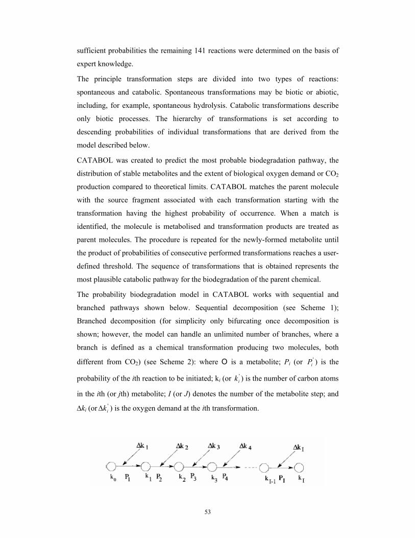
53

sufficient probabilities the remaining 141 reactions were determined on the basis of

expert knowledge.

The principle transformation steps are divided into two types of reactions:

spontaneous and catabolic. Spontaneous transformations may be biotic or abiotic,

including, for example, spontaneous hydrolysis. Catabolic transformations describe

only biotic processes. The hierarchy of transformations is set according to

descending probabilities of individual transformations that are derived from the

model described below.

CATABOL was created to predict the most probable biodegradation pathway, the

distribution of stable metabolites and the extent of biological oxygen demand or CO2

production compared to theoretical limits. CATABOL matches the parent molecule

with the source fragment associated with each transformation starting with the

transformation having the highest probability of occurrence. When a match is

identified, the molecule is metabolised and transformation products are treated as

parent molecules. The procedure is repeated for the newly-formed metabolite until

the product of probabilities of consecutive performed transformations reaches a user-

defined threshold. The sequence of transformations that is obtained represents the

most plausible catabolic pathway for the biodegradation of the parent chemical.

The probability biodegradation model in CATABOL works with sequential and

branched pathways shown below. Sequential decomposition (see Scheme 1);

Branched decomposition (for simplicity only bifurcating once decomposition is

shown; however, the model can handle an unlimited number of branches, where a

branch is defined as a chemical transformation producing two molecules, both

different from CO2) (see Scheme 2): where O is a metabolite; Pi (or 'iP ) is the

probability of the ith reaction to be initiated; ki (or 'ik ) is the number of carbon atoms

in the ith (or jth) metabolite; I (or J) denotes the number of the metabolite step; and

∆ki (or 'ik∆ ) is the oxygen demand at the ith transformation.

54

Scheme 1 (sequential decomposition) – Reprinted with permission from O.

Mekenyan.

Scheme 2 (branched decomposition) - Reprinted with permission from O.

Mekenyan.

Biodegradation expressed relative to the TOD, corresponding to these two types of

pathways, is described by the following equations.

Sequential decomposition:

I321TOD

I321

TOD

321

TOD

21

TOD

1 P..PPPk∆k...PPP

k∆kPP

k∆kP

k∆ky +++++= Eq. 5

where the TOD is defined as ∑ =∆=

I

i iTOD kk1

.

Branched decomposition:

'j

'321

TOD

j

'3

'21

TOD

'3

I321TOD

I21

TOD

21

TOD

1

P....PPPk∆k

...

PPPk∆k

P..PPPk∆k

...PPk∆k

Pk∆k

y

+

++++= Eq. 6

55

where the TOD is defined as ''3321 ... JITOD kkkkkkk ∆+∆+∆++∆+∆+∆=

and where Pi is the probability of the ith transformation to be initiated.

According to this model, the BOD yield (y), expressed as a percentage of TOD

(denoted as kTOD), is determined by summing the products of probabilities of the

respective transformations (Pi) and BOD yields at each metabolic step (∆ki).

Similar principal catabolic reactions (those yielding similar BOD and having similar

targets) are grouped and assumed to have the same probability. The hierarchy within

each subset of transformations with equal probability is able to reflect the effects of

neighbouring substituents. The hierarchy was set with expert knowledge. This

grouping into subsets was necessary to ensure numerical stability of the solutions

and to prevent overfitting the data with a model having too many degrees of

freedom. The probabilities are estimated, using the equations above, for all

chemicals in the training set.

Through the analysis of the pathway and its critical steps, based on individual

transformation probabilities, the CATABOL model enables the identification of

potentially persistent catabolic intermediates and their molar amounts.

The experimental values agreed well with the calculated BOD values (r2 = 0.69)

over the entire range (i.e. a good fit was observed for readily degradable,

intermediate, and difficult-to-degrade substances).

After introducing 60% TOD as a cut-off value, the model correctly predicted 86% of

the readily biodegradable structures and 91% of the not readily biodegradable

structures in the training set. Four-fold cross-validation, leaving out 25% of the data,

resulted in Q2 = 0.86 and 82% and 91% for ready/not ready correct classifications,

respectively.

The generated metabolic trees can also be used to evaluate the quantitative

distribution of the produced metabolites. The latter can be submitted for predicting

endpoints of interest, such as logKow, logBCF, fish acute toxicity, estrogen receptor

binding affinity, mutagenicity and other endpoints.

56

The development of CATABOL is ongoing and the most recent version of

CATABOL enable definition of the degree of membership of chemicals in the

domain of the biodegradation simulator.

7.3.5 TOPKAT

TOPKAT® is a computational tool developed by Accelrys [83] and is used by

universities, private companies and government agencies including the US EPA, US

FDA, Environment Canada, Health Canada and the Danish EPA for toxicity

assessments. It computes and validates assessments of the toxic and environmental

effects of chemicals solely from their molecular structure. TOPKAT employs robust

and cross-validated Quantitative Structure Toxicity Relationship (QSTR) models to

predict various measures of toxicity. The Optimum Prediction Space (OPS)

technology is implemented in TOPKAT as the methodology used to identify model

applicability domain, providing a means of cheking whether the compounds under

investigation are well represented in the models.

The recent release of TOPKAT 6.2 incorporates 16 modules (i.e. Aerobic

Biodegradability, Ames Mutagenicity, Daphnia Magna EC50, Developmental

Toxicity Potential, Fathead Minnow LC50, FDA Rodent Carcinogenicity, NTP

Rodent Carcinogenicity, Ocular Irritancy, Octanol/Water LogP, Rabbit Skin

Irritancy, Rat Chronic LOAEL, Rat Inhalation Toxicity LC50, Rat Maximum

Tolerated Dose (MTD), Rat Oral LD50, Skin Sensitisation, Weight-of-Evidence

Rodent Carcinogenicity).

The Aerobic Biodegradability Module of the TOPKAT® package consists of four

structurally based sub-models. It comprises a cross-validated quantitative structure-

toxicity relationship (QSTR) model applicable to a specific class of chemicals, and

the data from which these models were derived. A single study reporting the

biodegradability of 894 compounds, as assessed by the Japanese Ministry of

International Trade and Industry (MITI) I test protocol, was used to develop these

models. Molecular structure is the only input required to conduct the assessment of

aerobic biodegradability. The accuracy of the four structurally based sub-models is

illustrated in Table 3.

57

Chemical class N. of compounds

LOO validation

Accuracy %

Internal

Accuracy %)

Acyclics 317 96.1 97.7

Alicyclics 85 96.5 98.8

Single Benzenes 290 91.2 95.1

Multiple Benzenes and

Heteroaromatics 160 93.1 98.1

Table 3 – TOPKAT aerobic biodegradation model accuracy.

For this module, the discriminant models compute the probability of a submitted

structure of being capable of aerobic biodegradation (probability greater than 0.7) or

incapable of being degraded aerobically (probability below 0.3). Probability values

between 0.3 and 0.7 refer to an indeterminate region in which decisions should not

be made except in special circumstances or under further analytical assessments.

7.4 TGD models for persistence

In the European Union Technical Guidance Document (TGD) from 1996 for risk

assessment [12] the group contribution methods are regarded as the most applied and

successful way of modelling biodegradation. Since these models are based on a

direct link between molecular structure and biodegradability, they have the

possibility of straightforward interpretation.

The group contribution models suggested in the TGD are the multiple linear and

non-linear regression models incorporated in the Biodegradation Probability

Program (BIOWIN). Although objections can be made against the form of the

models, the accuracy and statistics, these models are considered usable with certain

restrictions. The combined use of Biowin1 (linear model) and Biowin2 (non-linear

model) is recommended.

The multiple linear (Biowin1) and non-linear (Biowin2) models have been validated

externally with MITI I test data (n=304) [85]. The differences between the

performances of Biowin1 and Biowin2 are small. The evaluation turned out that the

58

prediction “not ready degradable” is highly accurate (correct > 90% for both

Biowin1 and Biowin2), however the prediction “ready degradable” is frequently not

in agreement with experimental data obtained by the MITI I test. Therefore it is

recommended to use the results of BIOWIN only in a conservative way. If the

program predicts fast biodegradation, this estimate should not be taken into

consideration. However, if the program predicts slow biodegradation this can be

used as a confirmation of not readily biodegradable.

59

8. VALIDATION STUDIES ON BIODEGRADATION MODELS

8.1 BIODEG/PLS/MultiCASE/ Machine learning method validation on MITI-I

An extensive evaluation of general models for biodegradation was provided by

Sabljic and Peijnenburg in 2001 [42]. In this study, they analysed: a) the well known

Biodegradation Probability Program (BIODEG) [28]; b) the qualitative rule-based

inductive machine learning method developed by Gamberger et al [79]-[81]: c)

quantitative biodegradability models derived by partial least squares (PLS)

discriminant analysis [30]; and d) and the application of MultiCASE to select

structural fragments critical for biodegradability of organic compounds [59]-[60].

Models were evaluated in terms of their accuracy and range of applicability.

Particular emphasis was placed on the results of the external validation, and the main

limitations of the models were clearly described. Finally, recommendations were

provided on the reliable application of predictive models for estimating

biodegradability of organic chemicals in the environment.

8.1.1 BIODEG validation

In the validation study of biodegradation models, only the linear regression model

was evaluated. The linear BIODEG model was evaluated on a large set of consistent

biodegradation data of 733 compounds tested with the MITI-I test. The results were

considered to be realistic and a solid indicator of model’s future performance in

predicting biodegradability of new compounds, being based on a large set of

structurally diverse chemicals. The validation results [60] are summarised in Table 4.

The compounds used in model development and metalloorganic compounds were

excluded from the validation exercise. Results are presented for the original

threshold value (0.500) and optimised threshold value (0.803) of the BIODEG linear

model.

This result highlighted a relatively poor overall performance of the BIODEG model

(only 61.1% of correct predictions). Nevertheless, in the case of “ready”

biodegradable chemicals its predictivity was higher (91.1%).

60

Model BIODEG (0.500) BIODEG (0.803) N. Chemicals

Predicted "ready" "not ready" "ready" "not ready"

Correct 266 182 179 357 292 "ready"

Error 26 259 113 84 441 "not ready"

% correct 91.1 41.3 61.3 81.0

Table 4 – Number of chemicals predicted as “ready” or “not ready” biodegradable compared to the results of the MITI-I test.

However, the BIODEG model was not modelled to predict the outcome of the MITI-

I test, which was found to be a more strict measure of biodegradability than the

evaluated biodegradation data from the BIODEG dataset. Thus, it was considered

reasonable to find out that the BIODEG model predicts a significant number of

chemicals to be “ready” biodegradable although they were evaluated by MITI-I test

as “not ready” biodegradable chemicals. As described in Rorije et al. [60], it is

possible to correct this imperfection by changing the threshold value used to

distinguish between “ready” and “not ready” biodegradable chemicals to reflect the

evaluation of the MITI-I test instead of the Environmental Fate Database EFDB

evaluation. The optimised threshold value for the BIODEG linear model was found

to be 0.803, which improved the overall performance of the BIODEG linear model

to 73.1%. In addition, the number of correct predictions for the “not ready”

biodegradable chemicals was significantly improved, from 41.3% to 81.0%.

However, this improvement is reflected in a significant decease of the number of

correct predictions for the “ready” biodegradable chemicals, from 91.1% to 61.3%.

8.1.2 PLS biodegradation model validation

The PLS biodegradation model [30] was evaluated on the same large set of

consistent biodegradation data of 733 compounds tested with the MITI-I test used for

the BIODEG validation. The model was internally validated providing 85% of the

predictions in agreement with the observed biodegradability. “Not ready”

biodegradation was predicted slightly better, with 86% correct predictions vs. 84%

correct predictions for “ready” biodegradable substances. No predictions were

61

provided for about 10% of the substances because the calculated scores were in the

borderline area between “ready” and “not ready” biodegradation. Model predictions

for “not ready” biodegradable substances could be improved to 92%, by including

fragment–fragment interactions, but this did not improve predictions for “ready”

biodegradable substances. However, a real external validation by the simple use of

the MITI-I test protocol data could not be performed since all data were used to

develop the PLS model.

To provide a reasonable estimate of the predictivity of the model, the training set of

894 MITI-I test data was divided into four subsets consisting of 25% of substances

from the database. Four submodels without fragment–fragment interaction terms

were developed each time using three different subsets of chemicals. For each

submodel the remaining subset was used for external validation. The results of the

external validation of these four submodels are presented in Table 5.

Model N. Substances in validation

"Ready" Biodegradation

% correct predictions

"Not Ready" Biodegradation

% correct predictions

Total % correct predictions

Internal Validation 894 84% 86% 85%

Internal Validation + interactions

894 84% 92% 89%

Cross - Validation 1 223 79% 83% 81%

Cross - Validation 2 223 83% 84% 84%

Cross - Validation 3 224 81% 85% 83%

Cross - Validation 4 224 77% 87% 83%

Table 5 – Internal and external validation results.

62

The predictions for “not ready” biodegradation were in range of 83 to 87% correct,

and the predictions for “ready” biodegradation were 77 to 83% correct [30].

According to the results provided by Loonen et al. [30], the prediction scores of

internal and cross - validation are very similar and confirm a solid predictive

capability of the PLS model. Since the PLS model is a fragment based model, its

domain of application is unavoidably restricted by the presence of the fragments in

such substances. The PLS model was considered applicable to all substances having

at least one of the 127 fragments in their molecular structure. The broad range of

structural fragments used in developing the PLS model allows its application to a

wide variety of chemical structures.

8.1.3 MultiCASE model validation

The MultiCASE model was validated by using MITI-I test protocol data for 759

compounds [60], [86]. Of these chemicals, 630 had been used in model development.

The results of this study are given in Table 6.

The validation study highlighted that the MultiCASE model does not give a reliable

estimation of biodegradability, being able to correctly classify only a small fraction

of compounds not used in model development. The fact that the selection of

structural descriptors as performed by the MultiCASE model did not lead to a better

performance (compared to the PLS model) was attributed to the MLR

implementation of the selected fragments. If not carefully controlled, the high

number of structural descriptors used in the MLR approach may lead to overfitting

the data, resulting in a highly degraded performance in external validation.

63

Model MultiCASE (759) MultiCASE (630)

Predicted "ready" "not ready" All All

Correct 231 354 585 583

Error 84 90 174 48

% correct 73.3 79.7 77.1 92.5

Table 6 – Number of chemicals predicted as “ready” or “not ready” biodegradable compared to the evaluation in the MITI-I test of 759 chemicals.

The MultiCASE model was also applied to the same dataset of MITI-I values for 894

compounds used in the PLS study [30] in order to evaluate the capability of

MultiCASE variable selection to improve the classification of chemicals as “ready”

or “not ready” biodegradable. The dataset was divided into a training set of 643

chemicals and a test set of 251 chemicals. Eleven organometallic compounds and

two ambiguous structures were removed from the training set, which resulted in 630

chemicals for model development. This training set was again separated into two

files, one with all biodegradable compounds (n = 269) and one with all non-

biodegradable compounds (n = 361).

The test set of 251 compounds not used in the MultiCASE model development was

used to evaluate the ability of selected fragments (biophores and biophobes) to

correctly classify “ready” biodegradable and “not ready” biodegradable chemicals.

Seven organometallic compounds were excluded from this test set, leaving 244

compounds for evaluation. First, all compounds were searched for the presence of

biophores (sites of potential microbial attack). This search resulted in 41 warnings,

indicating compounds with structural fragments that may be potential biophores,

whereas none of those fragments were present in the training set compounds. In all

these cases, it was not possible to make predictions since the program does not try to

evaluate the effect of “unknown” fragments on biodegradability of those chemicals.

In addition, one compound was removed, being too small to contain any biophore.

The test set was reduced to 202 compounds. Due to the absence of a biophore, 106

compounds were predicted to be “not ready” biodegradable, which corresponded to a

64

correct prediction for 95 compounds (89.6%) according to their MITI-I values.

However, 96 compounds were predicted to be biodegradable due to the presence of a

biophore, but this was correct for only 43 of those chemicals (44.8%).

The test set of 244 compounds was then searched for biophobes (biodegradation-

retarding fragments). The second search resulted in 37 warnings on potential

biophobes reducing the test set to 207 compounds. Due to the presence of a

biophobe, 111 compounds were predicted to be “not ready” biodegradable, while 96

were predicted as “ready” biodegradable because of the absence of any known

biophobe. These results corresponded to correct predictions for 82 (73.9%) and 65

(67.7%) compounds, respectively.

8.1.4 Machine learning model validation

The inductive machine learning method developed by Gamberger et al [79]-[81] and

biodegradation data measured according to the MITI-I test protocol were used to

develop seven structural rules for “ready” biodegradable chemicals [42]. This set of

rules, based on 11 structural descriptors classified correctly 84.3% chemicals from

the training set of 762 compounds with a balanced predicted classifications of

“ready” (84.9%) and “not ready” (83.7%) biodegradable chemicals.

The set of developed rules was externally validated on 293 compounds from the

BIODEG database [28], [55]. The evaluation test showed that the overall

performance of the seven biodegradation rules is good since 85% of the predictions

were in agreement with the observed biodegradability. The predictions were slightly

better for “ready” biodegradable substances, with 86.3% correct predictions vs.

83.6% correct predictions for “not ready” biodegradable substances. The evaluation

test showed that the prediction scores on the training set and test sets were very

similar, providing evidence of the predictivity of the seven developed biodegradation

rules for “ready” biodegradable chemicals.

8.2 BIODEG/PLS/MultiCASE validation on HPVC

Rorijie et al. [60] analysed the similarities and diversities of the new and existing

biodegradation models (BIODEG/PLS/MultiCASE) based on structural fragments,

by comparing the most important descriptors of the models and their predictions for

65

a large dataset of High Production Volume Chemicals (HPVCs). The list of HPVCs

consisted of 2492 substances of which 1073 single compounds had a well defined

structural formula. These compounds were of interest for possible risk to the

environment by the European Union.

The four models were applied to make predictions for the 1073 single substances.

The BIODEG model could generate predictions for 918 of the compounds on the list

of HPVCs and provided 332 predictions for “ready biodegradable” and 586

predictions for “not ready”, using the optimised threshold value of 0.803. The

original threshold value of 0.5 yielded 610 “ready biodegradable” predictions and

308 “not ready” predictions.

The PLS model gave predictions for 924 compounds: 418 predictions for “ready

biodegradable” and 506 predictions for “not ready biodegradable”. The MultiCASE

model gave estimates for 885 compounds; 339 times “ready” and 546 times “not

ready”.

The differences between the predictions of the different models were evaluated in

terms of number of times the models predicted “ready biodegradability” for those

compounds containing the substructure fragments used as descriptors in the models.

It was commented that when one of the negative fragments was present in a

compound all models predict the majority of those compounds to be not ready

biodegradable. One exception was the aliphatic ether group, which was important in

the BIODEG model, and less important in the MultiCASE model.

Concerning the positive fragments it was noted that they were much more abundant

in the HPVCs, but they did not lead to high percentages of predictions of “ready

biodegradability”. Thus, a positive fragment was not a very strong indicator of ready

biodegradability. An important descriptor from the BIODEG model, the phosphate

group, was interpreted as an exception. In this case, the MultiCASE model and the

PLS model both predicted 0% of the compounds having this fragment to be ready

biodegradable.

8.3 BIODEG/OECD/PLS/MultiCASE validation on 894 MITI-I test

Rorijie et al. [60] also performed validated exercises on the BIODEG model [28], the

Degner et al. [52], Loonen PLS [30] and MultiCASE [59] biodegradation models,

using the larger set of consistent biodegradation data of 894 compounds tested with

66

MITI-I test for ready biodegradability. The overlap between the BIODEG training

set (295 compounds) and the MITI-I dataset resulted in 143 compounds.

The BIODEG model was used to predict the remaining 751 compounds in the MITI-

I dataset that were not in its training set: 18 of these were metallo-organic

compounds, thus the final dataset for validation resulted in 733 compounds.

The BIODEG model provided 61.1% of correct predictions: 50.7% of “ready

biodegradable” correct predictions (n=525) and 87.5% of “not ready biodegradable”

correct predictions (n=208). These results were found to be in agreement with the

previous validation results by Langenberg et al. [87] indicating that the prediction

“ready biodegradable” of this model is not reliable. However, the BIODEG model

was expected to predict too much compounds to be “ready biodegradable” since it

was never intended for predicting the outcome of the MITI-I test. The model was

originally optimised to generate a value of 1 for compounds evaluated as fast

biodegradable in the EFDB and a value of 0 for compounds evaluated to biodegrade

slowly, with a threshold value to distinguish the model prediction as “ready” or “not

ready” of 0.5. The optimised value to be used with the BIODEG linear regression

model to predict the MITI-I test was found to be 0.803. The overall performance of

the model at this optimal value was of 73.1% correct predictions. For the non-linear

model the optimal threshold value was determined to be 0.914, giving 72.6% correct

predictions overall.

The OECD models developed by Degner et al. are based on a representative dataset

of 65 and 60 compounds for the aliphatic and monoaromatic models, respectively,

taken from a dataset of 488 MITI-I test results. Since the compounds used in training

the models was unknown to Rorijie et al. [60], they used the complete dataset of 894

compounds for validation. The results of these validations are provided in Table 7.

BIODEG Degner et al. PLS MultiCASE

predicted RB N-RB RB N-RB RB N-RB RB N-RB

Actual RB 179 113 263 29 310 77 231 84

Actual N-RB 84 357 58 217 78 429 90 354

% correct: 68.1% 76.0% 81.9% 88.2% 80.0% 84.8% 72.0% 80.8%

67

Table 7 – Number of predictions "RB" = "ready biodegradable " or "N-RB" = "not ready biodegradable" compared to the evaluation in the MITI-I test.

It was highlighted that the good performance of the OECD models is due to the

selection of the compounds that can be predicted by the models. In fact, the total

number of predictions of the OECD models was always smaller than for the

BIODEG, PLS and MultiCASE model. The effect of this selection was evaluated

applying the BIODEG model on the subset of acyclic aliphatic compounds suitable

for prediction with the OECD model. In this case, the BIODEG gave a considerably

higher result (77.3% correct predictions of “ready biodegradable” and 82.6% correct

for the prediction “not ready biodegradable”) than that obtained using the complete

dataset.

8.4 BIOWIN/PLS/MultiCASE/CATABOL validation performance comparison

In a review by Nendza [71], the performance of the non-linear MITI-BIOWIN model

[77], MultiCASE/META [65], the PLS model [30], and the CATABOL model [69],

[88] were compared in terms of training and validation statistics.The statistics are

reported in Table 8.

The MITI-BIOWIN model was externally validated on the 295 MITI chemicals not

used for the model development. For the remaining models, validation results are

averages from four cross validations leaving out 25% of the data used in the training.

It was highlighted by Jaworska et al. [61] that the heterogeneity of the validation

methods and the different sizes of the training sets restrict in some way the

comparability of the performance of the models. Overall the models can provide

better predictions for non-readily biodegradable compounds. This was partly

explained by the fact that the presence of a biodegradation retarding fragment

prevent mineralisation, while a biodegradation enhancing fragment can point to a

possible metabolic step, but does not necessarily provide complete mineralisation.

Thus, a compound can be predicted as non-readily biodegradable because of a

structural fragment that is not present in the parent compound, but in one of the

possible metabolites from the transformation processes.

Thus, only if a compound is predicted non-degradable by the models, then it is likely

that it is really non-degradable and the prediction may be used with some reliance.

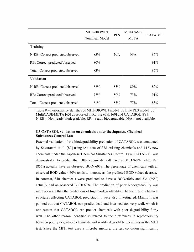
68

MITI-BIOWIN

Nonlinear Model PLS

MultiCASE/

META CATABOL

Training

N-RB: Correct predicted/observed 85% N/A N/A 86%

RB: Correct predicted/observed 80% 91%

Total: Correct predicted/observed 83% 87%

Validation

N-RB: Correct predicted/observed 82% 85% 80% 82%

RB: Correct predicted/observed 77% 80% 73% 91%

Total: Correct predicted/observed 81% 83% 77% 83%

Table 8 – Performance statistics of MITI-BIOWIN model [77], the PLS model [30], MultiCASE/META [65] as reported in Rorijie et al. [60] and CATABOL [88]. N-RB = Non-ready biodegradable; RR = ready biodegradable; N/A = not available.

8.5 CATABOL validation on chemicals under the Japanese Chemical Substances Control Law

External validation of the biodegradability prediction of CATABOL was conducted

by Sakuratani et al. [89] using test data of 338 existing chemicals and 1123 new

chemicals under the Japanese Chemical Substances Control Law. CATABOL was

demonstrated to predict that 1089 chemicals will have a BOD<60%, while 925

(85%) actually have an observed BOD<60%. The percentage of chemicals with an

observed BOD value <60% tends to increase as the predicted BOD values decrease.

In contrast, 340 chemicals were predicted to have a BOD>60% and 234 (69%)

actually had an observed BOD>60%. The prediction of poor biodegradability was

more accurate than the predictions of high biodegradability. The features of chemical

structures affecting CATABOL predictability were also investigated. Mainly it was

pointed out that CATABOL can predict dead-end intermediates very well, which is

one reason that CATABOL can predict chemicals with poor degradability fairly

well. The other reason identified is related to the differences in reproducibility

between poorly degradable chemicals and readily degradable chemicals in the MITI

test. Since the MITI test uses a microbe mixture, the test condition significantly

69

depends on the variability in the inocula. In addition, BOD by its definition is not

directly related to biodegradation. These factors limit the accuracy of CATABOL

predictions for readily biodegradable chemicals. This superiority in predicting

chemicals with poor biodegradability compared to predicting chemicals that readily

biodegrade was also reported by Tunkel et al. [77] for BIOWIN models, which are

based on CSCL data.

70

9. CONCLUSIONS

The major obstacle for the development of reliable biodegradation models in the past

was the absence of standardised and uniform biodegradation data for different

chemical classes. The availability of databases of high quality biodegradation

screening test data concerning ready biodegradation, BIODEG and MITI-I, led to an

intensive development of advanced computational and statistical methods. The group

contribution approach (BIOWIN), the expert system approach (META, BESS) and a

combination of expert system and probabilistic modelling of pathways (CATABOL)

are the most commonly used approaches for estimating biodegradation of organic

compounds. The group contribution method has the advantage of being a simple

approach that has been shown to predict well biodegradation rates, although the

calculated probabilities cannot be used to identify degradation pathways. On the

other hand, this approach is strongly dependent on the choice of preselected

fragments and takes into account only on the structure of the parent compound.

The expert system approaches are generally more complex methods and their

predictions are strongly dependent on the transformation library. The

MutliCASE/META approach is a mixture of a group contribution model and an

expert system since it neutrally sets the hierarchy of transformations associated with

biophores from their fragment contributions. This modelling approach is based on

the parent compound solely. The CATABOL system is also a hybrid system of

pathway prediction and transformation probability modelling which explicitly takes

into account the effect of adjacent fragments.

Overall the models are more reliable for predicting no ready-biodegradability, than

ready degradability. This can to a certain extent be explained by the consideration

that the presence of a biodegradation retarding fragment prevents mineralization,

while a biodegradation enhancing fragment generally indicates a possible metabolic

step, which does not necessarily lead to a complete mineralization. No-readily

biodegradation might be a consequence of a structural fragment that is not present in

the parent compound but in one of the metabolites. Therefore, it is frequently

accepted that only if a compound is predicted not-ready degradable by the models,

then there is a good probability that it is really not-degradable and the predicted

results are considered reliable.

71

After Sabljic and Peijnenburg’s recommendation in 2001 [42] to focus on

developing broadly applicable models, several works have been published in the

biodegradation field. However, further research in modelling techniques is needed to

obtain models capable to reliable predict biodegradability of chemicals that are

significantly different from those used to develop the models.

To this end, there is the need for additional high-quality quantitative biodegradation

data on structurally diverse chemicals.

Further understanding of the role of metabolites in biodegradation is essential as well

as the identification of specific metabolites that might represent a potential issue. As

a consequence there is a strong need of models capable of predicting metabolites and

their hazard profile to be used to support risk assessment and to guide it in the

development of testing and screening strategies.

Concerning the modelling techniques, hybrid combinations of expert systems and

quantitative models are becoming widespread, due to the fact that they can take

advantages of modelling algorithms and avoid the restrictions of any single

approach.

Finally, a recommended procedure for estimating biodegradation in the environment

might be based on consensus modelling, i.e. using a set of models in combination, in

a parallel and/or sequential manner.

72

10. REFERENCES [1]. European Commission (2003). Proposal for a Regulation of the European

Parliament and of the Council concerning the Registration, Evaluation, Authorisation and Restriction of Chemicals (REACH), establishing a European Chemicals Agency and amending directive 1999/45/EC and Regulation (EC) {on Persistent Organic Pollutants} [http://europa.eu.int/comm/enterprise/reach/overview_en.htm].

[2]. European Commission (2001). White Paper on a Strategy for a Future Chemicals Policy. Brussels: Commission of the European Communities (COM(2001) 88 final), 32pp. Belgium, Brussels: the Commission of the European Communities. (http://europa.eu.int/comm/environment/chemicals/whitepaper.htm).

[3]. Nendza M (2004). Prediction of Persistence. In: Cronin, M.T.D. and Livingstone, D.J. eds, Predicting Chemical Toxicity and Fate. CRC Press, Boca Raton, FL, 315-331.

[4]. Mackay D, Fraser A. (2000). Bioaccumulation of persistent Organic Chemicals: mechanisms and Models. Environmental Pollution, 110, 375-391.

[5]. UNEP, United Nations Environmental Program (1972), Environmental Conference on the Human Environment, Stockholm (http://www.unep.org/Documents.Multilingual/default.asp?documentid=97&l=en).

[6]. United Nations (1992). Agenda 21 – United Nations conference on Environment and Development. Rio de Janeiro, Brazil, 3-14 June 1992 (http://www.un.org/esa/sustdev/documents/agenda21/).

[7]. UNEP, United Nations Environmental Program (1995), Governing Council Decision 18/32, Nairobi, May 1995.

[8]. UNEP, United Nations Environmental Program (1997), Governing Council Decision 19/13C, Nairobi, February 1997.

[9]. UNEP, United Nations Environmental Program (2001), Stockholm Convention on Persistent Organic Pollutants, Geneva, October 2001.

[10]. OSPAR Commission (1998). OSPAR Strategy with regard to Hazardous Substances (http://www.defra.gov.uk/environment/chemicals/csf/10092002/pdf/csf-inf-02-22.pdf).

[11]. OSPAR Commission (2002). Provisional Instruction Manual for the Dynamic Selection and Prioritisation Mechanism for Hazardous Substances (DYNAMEC).

[12]. European Commission (2003). Technical Guidance Document on Risk Assessment in support of Commission Directive 93/67/EEC on Risk Assessment for new notified substances, Commission Regulation (EC) No 1488/94 on Risk Assessment for existing substances, and Directive 98/8/EC of the European Parliament and of the Council concerning the placing of biocidal products on the market.

73

[13]. European Commission (2001). Proposal for a European Parliament and Council Decision establishing the list of priority substances in the field of water policy; 7 February 2000 (COM(2000) 47 final) as amended on 16 January 2001 (COM(2001) 17 final).

[14]. PBT Profiler Developed by the Environmental Science Center under contract to the Office of Pollution Prevention and Toxics, U.S. Environmental Protection Agency, Computer Resources Donated by Syracuse Research Corporation Ver 1.203 (available at www.pbtprofiler.net).

[15]. Pollution Prevention (P2) Framework. (http://www.epa.gov/opptintr/p2framework/).

[16]. Canada Gazette (2000). Persistence and Bioaccumulation Regulations. Canada Gazette, Part II, Vol 134. No. 7.

[17]. Government of Canada (1995). Toxic Substances Management Policy: Persistence and Bioaccumulation Criteria. Final Report of the ad hoc Science Group on Criteria.

[18]. Law Concerning the Evaluation of Chemical Substances and Regulation of Their Manufacture. Law No. 117, October 16, 1973 as last amended by Law No.49 May 28, 2003. www.safe.nite.go.jp/english/kasinn/pdf/PROVISIONALTRANSLATION_L1.pdf

[19]. BIOWIN program is available from the US EPA's internet site (http://www.epa.gov/oppt/exposure/docs/episuitedl.htm).

[20]. Howard PH, Banerjee S. (1984). Interpreting results from biodegradability tests of chemicals in water and soil. Environmental Toxicology and Chemistry, 3, 551–562.

[21]. Howard P (2000). Biodegradation. In Boethling, R., Mackay, D. eds Handbook of Property Estimation Methods for Chemicals. Lewis, Boca Raton, FL, USA, pp. 281-310.

[22]. Voustas E., Magoulas K., Tassios D. (2002). Prediction of bioaccumulation of persistent organic pollutants in aquatic food webs. Chemosphere, 48, 645-651.

[23]. European Centre for Ecotoxicology and Toxicology of Chemicals (1995). The Role of Bioaccumulation in Environmental Risk Assessment: The Aquatic Environment and Related Food Webs. Technical report 67, Brussels, Belgium.

[24]. OECD (1981). Organisation for Economic Cooperation and Development, Guide-Line for testing of Chemicals: Bioaccumulation, Paris, France, 1981.

[25]. Gobas FAPC, Zhang X. (1995). Measuring bioconcentration factors and rate constants of chemicals in aquatic organism under condition of variable water concentration and short exposure time. Chemosphere, 25, 1961-1971.

[26]. Nendza M (1998). Structure–Activity Relationships in Environmental Sciences, Chapman & Hall, London.

[27]. Pavan M, Worth AP, Netzeva TI (2006). Review of QSAR Models for Bioconcentration. JRC report EUR EN. European Chemicals Bureau, Ispra, Italy. Available from: http://ecb.jrc.it.

74

[28]. Howard P, Meylan W (1992). Biodegradation Probability Program (BIODEG), Version 3. Syracuse Research Corporation. Syracuse, NY, USA.

[29]. Syracuse Research Corporation, Environmental Fate Data Base, Syracuse, NY, USA (1995). (http://www.syrres.com/esc/biodeg.htm).

[30]. Loonen H., Lindgren F, Hansen B, Karcher W. (1996). Biodegradability Prediction. Kluwer Academic Publishers, Dordrecht, pp. 105-114.

[31]. Takatsuki M, Takayanagi Y, Kitano M. In: Proceedings of the Workshop “Quantitative Structure Activity Relationships for Biodegradation”, W. J. G. M. Peijnenburg and W. Karcher (Eds.), pp. 67-103, National Institute of Public Health and Environmental Protection, Bilthoven (1995).

[32]. Chemicals Investigation and Testing Institute (1992). Biodegradation and Bioaccumulation Data of exiting Chemicals Based on the CSCL Japan, ISBN 4-98074-101-1. Japan Chemical Industry Ecology-Toxicology & Information Center.

[33]. OECD (1994). Organisation for Economic Cooperation and Development. OECD guidelines for the Testing of Chemicals, Guideline 310. Ready Biodegradability, Paris .

[34]. Office of Prevention, Pesticides and Toxic Substances (1998). Ready Biodegradability, Part 835.3110 in OPPTS Harmonized Test Guidelines, UPA 712-C98_076 (US Government Printing Office, Washington, DC).

[35]. European Community. Biodegradation: determination of “ready’ biodegradability; carbon dioxide (CO2) evolution. Official Journal of the European Communities, 35 (L 383 A), 202-206, ISSN 0378-6978.

[36]. Chemicals Inspection and Testing Institute Japan. Data of Existing Chemicals Based on the CSCL Japan. Japan Chemical Industry Ecology-Toxicology and Information Center, Fukuoka (1992).

[37]. Ellis LBM, Roe D, Wackett LP (2006). The University of Minnesota Biocatalysis/Biodegradation Database: The First Decade. Nucleic Acids Research 34: D517-D521.

[38]. Alexander M (1999). Biodegradation and Bioremediation, 2nd ed. Academic, New York, NY, USA.

[39]. Pitter P, Chudoba J (1990). Biodegradability of Organic Substance in Aquatic Environment. CRC, Boca Raton, FL, USA.

[40]. Hermens J, Balaz S, Damborsky J, Karcher W, Müller M, Peijnenburg W, Sabljic, A, Sjöström,M (1995). Assessment of QSARs for predicting fate and effects of chemicals in the environment: An international European project. SAR and QSAR in Environmental Research 3, 223–236.

[41]. Güsten H, Medven Z, Sekusak S, Sabljic A (1995). Predicting tropospheric degradation of chemicals: from estimation to computation. SAR and QSAR in Environmental Research 4, 197–209.

[42]. Sabljic A, Peijnenburg W (2001). Modeling lifetime and degradability of organic compounds in air, soil, and water systems. IUPAC Pure and Applied Chemistry, 73, 1331-1348.

75

[43]. Niemi J, Veith G, Regal R, Vaishnav D (1987). Structure features associated with degradable and persistent chemicals, Environmental Toxicology and Chemistry, 6, 515-527.

[44]. Boethling R (1986). Application of molecular topology to quantitative structure—biodegradability relationships, Environmental Toxicology and Chemistry, 5, 797-806.

[45]. Parson JR, Govers HAJ (1990). Quantitative structure—activity relationships for biodegradation, Ecotoxicology and Environmental Safety, 19, 212-227.

[46]. Howard PH (2000). Biodegradation. In Boethling RS, Mackay D. eds, Handbook of Property Estimation Methods for Chemicals. Lewis, Boca Raton, FL, USA, 281-310.

[47]. Yonezawa Y, Urushigawa Y (1979). Chemico-biological interactions in biological purification systems V. Relation between biodegradation rate constants of aliphatic alcohols by activated sludge and their partition coefficients in a 1-octanol-water system. Chemosphere, 8, 139-142.

[48]. Yonezawa Y, Urushigawa Y (1979). Chemico-biological interactions in biological purification systems VI. Relation between biodegradation rate constants of di-n-alkyl phthalate esters and their retention times in reverse phase partition chromatography. Chemosphere, 8, 317-320.

[49]. Banerjee S, Howard PH, Rosenberg AM, Dombrowski AE, Sikka H, Tullis DL (1984). Development of a general kinetic model for biodegradation and its application to chlorophenols and related compounds. Environmental Science & Technolgy, 18, 416 – 422.

[50]. Paris DF, Wolfe NL, Steen WC, Baughman GL (1983). Effect of Phenol Molecular Structure on Bacterial Transformation Rate Constants in Pond and River Samples. Applied and Environmental Microbiology, 45, 1153–1155.

[51]. Paris DF, Wolfe NL (1987). Relationship between properties of a series of anilines and their transformation by bacteria. Applied and Environmental Microbiology, 53(5), 911–916.

[52]. Degner P, Müller M, Nendza M, Klein W (1993). Structure-Activity Relationships for Biodegradation. Organisation for Economic Cooperation and Development (OECD), OECD Environment Monographs No 68, Paris.

[53]. Langenberg J.H, Peijnenburg W.J.G.M, Rorije E. (1996). On the usefulness and reliability of existing QSBRs for risk assessment and priority setting. SAR and QSAR in Environmental Research, 5, 1-16.

[54]. Rorije E, Langenberg JH., Peijnenburg WJGM. (1995). QSARs for biodegradation. In: Overview of Structure-Activity Relationships for Environmental Endpoints, Part 1: General Outline and Procedure. Hermens JLM (ed.), Report prepared within the framework of the project “QSAR for Prediction of Fate and Effects of Chemicals in the Environment”, an international project of the Environmental Technologies RTD Programme (DGXII/D-1) of the European Commission under contract number EV5V-CT92-0211.

[55]. Howard PH, Boethling RS, Stiteler WM, Meylan WM, Hueber AE, Beauman JA, Larosche ME (1992). Predictive model for aerobic biodegradability

76

developed from a file of evaluated biodegradation data. Environmental Toxicology and Chemistry, 11, 593-603.

[56]. Degner P, Muller M, Nendza M, Klein W (1993). Structure —Activity Relationships for Biodegradation, OECD Environment Directorate, Paris.

[57]. Boethling RS, Howard PH, Meylan WM, Stiteler WM, Beauman JA, Tirado N (1994). Group contribution method for predicting probability and rate of aerobic biodegradation. Environmental Science & Technology, 28, 459-465.

[58]. Tabak HH, Govind, R (1993). Prediction of biodegradation kinetics using a nonlinear group contribution method. Environmental Toxicology and Chemistry, 12, 251—260.

[59]. Klopman G (1992). MultiCASE: A hierarchical computer automated structure evaluation program, Quantitative Structure-Activity Relationship, 11, 176—184.

[60]. Rorije E, Loonen H, Muller M, Klopman G, Peijnenburg WJGM (1999). Evaluation and application of models for the prediction of ready biodegradability in the MITI-I test, Chemosphere, 38, 1409-1417.

[61]. Jaworska JS, Boethling RS, Howard PH (2003). Recent developments in broadly applicable structure-biodegradability relationships. Environmental Toxicology and Chemistry, 22 (8), 1710-1723.

[62]. Grammatica P, Pavan M, Consolaro F, Connsonni V, Todeschini R (2000). QSAR modeling of the biodegradation by holistic molecular descriptors. Abstracts, 9th International Workshop on QSARs, Bourgas, Bulgaria, September 16-20, p 36.

[63]. Leardi R, Boggia R, Terrile M. (1992). Genetic algorithms as a strategy for feature selection. Journal of Chemometrics, 6, 267-281.

[64]. Kubinyi H (1996). Evolutionary variable selection in regression and PLS analysis. Journal of Chemometrics, 10, 119-133.

[65]. Klopman G, Tu M (1997). Structure—biodegradability study and computer-automated prediction of aerobic biodegradation of chemicals. Environmental Toxicology and Chemistry, 16, 1829-1835.

[66]. Klopman G, Dimayuga M, Talafous J (1994). META: 1. A program for evaluation of metabolic transformation of chemicals. Journal of Chemical Information and Computer Sciences, 34, 1320-1325.

[67]. Klopman G, Zhang Z, Balthasar DM, Rosenkranz HS (1995). Computer-automated prediction of aerobic biodegradation transformation in the environment. Environmental Toxicology and Chemistry, 14, 395-403.

[68]. Klopman G, Tu M, Talafous J (1997). Meta 3 A genetic algorithm for metabolic transform priorities optimization, Journal of Chemical Information and Computer Sciences, 37, 329-334.

[69]. Jaworska J, Dimitrov S, Nikolova N, Masscheleyn P, Mekenyan O (2002). Probabilistic Assessment of Biodegradability Based on Metabolic Pathways: CATABOL System. In: Mekenyan O. and Schultz T.W (eds.) Proceedings of Quantitative Structure Activity Relationships in Environmental Sciences - I 2002, SAR and QSAR in Environmental Research, 13, 307-323.

77

[70]. Dimitrov S, Kamenska V, Walker JD, Windle W, Purdy R, Lewis M, Mekenyan O (2004). Predicting the Biodegradation Products of Perfluorinated chemicals using CATABOL. SAR and QSAR in Environmental Research, 15 (1) 69-82.

[71]. Nendza M (2004). Prediction of Persistence In: Cronin, M.T.D. and Livingstone, D.J. eds, Predicting Chemical Toxicity and Fate. CRC Press, Boca Raton, FL, 315-331.

[72]. Degner P, Müller M, Nendza M, Klein W (1993). Structure-Activity Relationships for Biodegradation. OECD Environment Monograph N.68, Paris, France.

[73]. Loonen H, Lindgren F, Hansen B, Karcher W, Niemelä J, Hiromatsu K, Takatsuki M, Peijnenburg W, Rorije E, Struij J (1999). Prediction of biodegradability from chemical structure modeling of ready biodegradation test data. Environmental Toxicology and Chemistry, 18, 1763-1768.

[74]. Eakin DR, Hyde E, Palmer G (1974). The use of computers within chemical structure information: the ICI CROSSBOW system. Pesticide Science, 5, 319-326.

[75]. Howard PH, Hueber AE, Boethling RS (1987). Biodegradation data evaluation for structure/biodegradability relations. Environmental Toxicology and Chemistry, 6, 1-10.

[76]. Boethling RS, Sabljic A (1989). Screening-level model for aerobic biodegradability based on a survey of expert knowledge. Environmental Science and Technology, 23, 672-679.

[77]. Tunkel J, Howard PH, Boethling RS, Stiteler W, Loonen H (2000). Predicting Ready Biodegradability in the Japanese Ministry of International Trade and Industry Test. Environmental Toxicology and Chemistry, 19, 2478-2485.

[78]. Boethling RS, Lynch, DG, Jaworska JS, Tunkel JL, Thom GC, Webb S (2004). Using BIOWIN, Bayes, and batteries to predict ready biodegradability. Environmental Toxicology and Chemistry, 23, 911-920.

[79]. Gamberger D, Hoevaric D, Sekusak S, Sabljic A (1996). Application of expert’s judgements to derive structure-biodegradation relationships. Environmental Science and Pollution Research, 3, 224-228.

[80]. Gamberger D, Sekusak S, Medven Z, Sabljic A. (1996). In: Biodegradability Prediction, W.J.G.M. Penijnenburg and J.Damborsky (Eds.), p.41-50, Kluwer, Dordrecht (1996).

[81]. Gamberger D, Sekusak S, Sabljic A (1996). Modelling biodegradation by an example-based learning system. Informatica, 17, 57-166

[82]. Punch B, Patton A, Wight K, Larson RJ, Masscheleyn P, Forney L (1996). A biodegradability evaluation and simulation system (BESS) based on knowledge of biodegradation pathways. In Biodegradability Prediction, W.J.G.M. Penijnenburg and J.Damborsky (Eds.), p.65-73, Kluwer, Dordrecht (1996).

[83]. Topkat Version 6.2. Accelrys. http://www.accelrys.com/products/topkat/

78

[84]. Dimitrov SD, Dimitrova NC, Jaworska J, Federle T, Mekenyan O (2002). Simulating biodegradability in ready tests. Proceeding, 10th Workshop on QSARs in Environmental Sciences, Ottawa, ON, Canada, May 26-29, p. 13.

[85]. Pederson F, Tyle H, Niemelä JR, Guttman B, Lander L, Wedebrand A (1994). Environmental Hazard Classification - Data Collection and Interpretation Guide for Substances to be Evaluated for Classification as Dangerous for the Environment. Appendix 9: Validation of the BIODEG Probability Program. TemaNord Report 589, 153-156.

[86]. Chemicals Inspection and Testing Institute Japan. Data of Existing Chemicals Based on the CSCL. Japan. Japan Chemical Industry Ecology-Toxicology and Information Center, Fukuoka (1992).

[87]. Langenberg JH, Peijnenburg WJGM, Rorije E (1996). On the usefulness and reliability of existing QSBRs for risk assessment and priority setting, SAR and QSAR in Environmental Research, 5, 1-16.

[88]. Dimitrov S, Breton R, MacDonald D, Walker JD, Mekenyan O (2002). Quantitative prediction of biodegradability, metabolic distribution and toxicity of stable metabolites. SAR and QSAR in Environmental Research, 13, 445-455.

[89]. Sakuratani, Y., Yamada, J., Kasai, K., Noguchi, Y., Nishihara, T. (2005). External validation of the biodegradability prediction model CATABOL using data sets of existing and new chemicals under the Japanese Chemical Substances Control Law. SAR and QSAR in Environmental Research, 16, 403-431

European Commission EUR 22355 EN – DG Joint Research Centre, Institute for Health and Consumer Protection Review of QSAR Models for Biodegradation Pavan, Manuela, Worth, Andrew Luxembourg: Office for Official Publications of the European Communities 2006 – 78 pp. – 21x 29.7 cm EUR - Scientific and Technical Research series; ISSN 1018-5593 Abstract Many regulatory laws resulting from the enactment of the United Nations Stockholm Convention in May 2004, together with the new REACH legislation, have promoted significant new activity in the assessment of Persistent, Bioaccumulative and Toxic (PBT) substances. These are chemicals that have the potential to persist in the environment, accumulate within the tissues of living organisms and, in the case of chemicals categorised as PBTs, show adverse effects following long-term exposure. Under REACH, estimated data generated by (Q)SARs may be used both as a substitute for experimental data, and as a supplement to experimental data in weight-of-evidence approaches. It is foreseen that (Q)SARs will be used for the three main regulatory goals of hazard assessment, risk assessment and PBT/vPvB assessment. In the Registration process under REACH, the registrant will be able to use (Q)SAR data in the registration dossier, provided that adequate documentation is given to argue for the validity of the model(s) used. The experimental determination of the persistence, bioconcentration and toxicity is generally expensive and demanding to perform. For this reason, measuring experimentally the potential PBT profiles of those chemicals that are of potential regulatory interest is considered not feasible. The limited empirical data, the high test costs together with the regulatory constraints and the international push for reduced animal testing motivates a greater reliance on QSAR models in PBT assessment. This report provides an overview of PBT regulations and criteria, and gives a detailed review of QSAR for estimating the biodegradation of chemicals. The role of biotransformation in the modelling of PBT substances is also described.

The mission of the JRC is to provide customer-driven scientific and technical support for the conception, development, implementation and monitoring of EU policies. As a service of the European Commission, the JRC functions as a reference centre of science and technology for the Union. Close to the policy-making process, it serves the common interest of the Member States, while being independent of special interests, whether private or national.