Paulson’s Gift

Pietro Veronesi* University of Chicago, NBER & CEPR

Luigi Zingales*

University of Chicago, NBER & CEPR

October, 2009

Abstract

We calculate the costs and benefits of the largest ever U.S. Government intervention in the financial sector announced the 2008 Columbus-day weekend. We estimate that this intervention increased the value of banks’ financial claims by $131 billion at a taxpayers’ cost of $25 -$47 billions with a net benefit between $84bn and $107bn. By looking at the limited cross section we infer that this net benefit arises from a reduction in the probability of bankruptcy, which we estimate would destroy 22% of the enterprise value. The big winners of the plan were the three former investment banks and Citigroup, while the loser was JP Morgan.

*University of Chicago Booth School of Business, National Bureau of Economic Research and Center for Economic Policy Research. We thank Douglas Diamond, Ralph Koijen, Neill Pearson, Jeremy Stein for very helpful comments, Francesco D’Acunto and Federico De Luca for excellent research assistantship, and Peggy Eppink for editorial assistance. Luigi Zingales thanks the IGM center at the University of Chicago for financial support.

2

The 2008 financial crisis witnessed the largest intervention of the U.S. government in the

financial sector. The stated goal of this intervention was to “restore confidence to our

financial system”, 1 through a massive transfer of resources from the taxpayers to the

banking sector. From an economic point of view, such an intervention is justified only in

the presence of a market failure that the government could help alleviate. If this market

failure is present, then the government intervention should create, not just redistribute,

value. Did this intervention create value or was it simply a massive transfer of resources

from taxpayers to financial institutions? If it did create value, why? What can we learn

about the possible cost of financial distress in financial institutions?

To answer these questions we estimate the costs and benefits of the largest U.S.

government intervention into the financial sector, announced on Monday, October 13,

2008. The plan included a $125bn preferred equity infusion in the nine (ten if we

consider Wachovia still independent) largest U.S. commercial banks joined by a three

year Government guarantee on new unsecured bank debt issues. For brevity, throughout

the paper we refer to the U.S. Treasury – FDIC joint plan as the “Paulson’s Plan,” after

the name of the then U.S. Treasury Secretary, Hank Paulson.

Given the worldwide changes in financial markets occurring between Friday the

10th and Tuesday the 14th, it is impossible to estimate the systemic effects of the

intervention. However, it is possible to estimate its effects on the banks involved. If the

intervention stopped a bank run, for instance, it should have created some value in the

banking sector. To compute the intervention’s effect on the value of banks we do not

limit ourselves to the changes in the value of common and preferred equity, but we look

at the changes in the entire enterprise value by looking also at changes in the value of

existing debt. In fact, by using liquid credit default swap (CDS) rates, we introduce a new

way to perform event studies on debt.

To separate the effect of the Paulson Plan from that of other events occurring at

the same time, we control for the change in the CDS rates of GE Capital, the largest non-

bank financial company. This difference-in-difference approach estimates the total

increase in debt value due to the plan at $119bn. If we add to these changes, the abnormal

1 Statement by Secretary Henry M. Paulson, Jr. on Actions to Protect the U.S. Economy, October 14, 2008. http://www.financialstability.gov/latest/hp1205.html.

3

variation in the market value of common equity (-$2.8bn) and of preferred equity

(+$6.7bn), we obtain that the enterprise value of the 10 banks involved in the first phase

of the plan increased by $128bn. If we add the value increase in the derivative liabilities

and the reduction in the value of the FDIC deposit guarantee, we come to a total increase

of $131bn.

This increase, however, came at a cost to the taxpayers. By computing the value

of the preferred equity and the warrants the Government will receive in exchange for the

$125bn investment we obtain an estimate between $89 and $112 bn. Hence, the preferred

equity infusion costs taxpayers between $13bn and $36bn. We also estimate the cost of

the debt guarantee extended by the FDIC on all the new bank debt to be worth $11bn.

This brings the total taxpayers’ cost at between $25bn and $47bn. Hence, the plan added

between $84 and $107 billion in value. Even if we account for a 30% deadweight cost of

taxation (see Ballard et al. 1985, and Feldstein, 1999), the plan created between $71bn

and $89bn in value.

Where does this added value come from? What friction did the plan help to

resolve? Who are the main beneficiaries of the plan?

To address these questions we exploit the (very small) cross section of results at

our disposition. We find that the bulk of the value added stems from the banks that were

more at risk of a run. For each bank, we compute a “bank run” index, which measures the

difference between the (risk neutral) probability of default in the immediately following

year and the (risk neutral) probability of default between year 1 and year 2, conditional

on surviving at the end of year one. When this index is large it means that investors

believe that the bank is very likely to default soon.

We find a very high correlation (96%) between the ex-ante value of the bank run

index and the percentage increase in a bank enterprise value at the announcement of the

plan. The big beneficiaries of the intervention were the three former investment banks

and Citigroup, while the loser was JP Morgan whose total asset value decreased even

before the benefit of the Paulson plan is accounted for. This result is not so paradoxical.

In spite of the benefits of the Paulson plan, banks might lose value because their

participation provides a negative signal to the market about the true value of the assets in

4

place, because the government future interference in banks’ affair reduces value, or

because intervention has redistributive effects across banks.

Since all the major banks were “forced” to participate by a very strong arm-

twisting exercised by Treasury Secretary Paulson, it is unlikely that participation might

signal any inside information about the value of the assets in place. A more realistic

interpretation is that the government intervention has two conflicting effects: a negative

one linked to the government future interference in banks’ affairs, and a positive one,

associated with the reduction in the probability of bankruptcy and hence the expected

cost of bankruptcy. Exploiting the firm variation in this latter probability, we estimate

that the expected cost of government interference is about 2.5% of enterprise value, while

the cost of bankruptcy is about 22% of enterprise value.

Given the extreme volatility of markets during this period one may wonder

whether the observed outcome represents a fair assessment of the intervention’s effects.

For this reason, we evaluate the plan on an ex ante basis by using the standard Black and

Scholes (1973) and Merton (1974) model of equity as an option on the value of the

underlying assets. When we keep the assets’ value constant (i.e., the intervention neither

creates nor destroys any value) the model grossly underestimates the market response.

According to the model, the shareholders should have lost $25bn and instead lost only

$3bn. The debtholders should have gained $49bn and instead gain $119. To bridge this

difference we need to hypothesize an increase in the value of the underlying assets. It is

only if we assume an increase in the value of assets of $113bn that the model can

approximate well the actual changes in the value of debt and equity. This alternative

method confirms the magnitude of the asset increase.

Finally, we try to evaluate whether the same objective achieved by the plan could

have been obtained at a lower cost to taxpayers. If the main goal was to make banks

solvent, we assume that the objective is to achieve a reduction in the CDS rates

equivalent to the one observed in the data after the plan. We analyze four alternative

plans: the original Paulson plan where bank’s assets were purchased at market value, the

original Paulson plan with bank’s assets purchased above market (we assume a 20%

above), a British-style equity infusion without any debt guarantee, and a debt-for-equity

swap. We rate these alternatives on the basis of up-front investment required by the

5

Government, taxpayers’ expected cost, taxpayers’ value at risk, and Government

ownership of banks. While expensive with respect to a debt-for-equity swap, we find that

the revised Paulson plan strikes a reasonable compromise in terms of the various cost

metrics.

The rest of the paper proceeds as follows. Section 1 describes the 2008financial

crisis and discusses the potential reasons for a government intervention. It also describes

the details of the plan announced by U.S. Treasury and FDIC on October 13, 2008.

Section 2 analyzes the effect of the plan on the prices of the bonds, the common equity,

and the preferred. Section 3 computes the net cost of the preferred equity infusion and the

debt guarantee. Section 4 analyzes the plan from an ex ante point of view. Section 5

studies the cost of alternative plans that would have achieved the same objective.

Conclusions follow.

1. The 2008 Financial Crisis and Rationale of Government Intervention

In this section we analyze the financial environment in the weeks before the

announcement, and the likelihood of possible inefficiencies that would justify the

Government action. We then detail the government response in October 2008.

1.1 Debt Overhang

The events leading up to the massive government intervention on 10/14/2008

strongly suggest that banks were reluctant to provide credit to individuals and

corporations independently of their creditworthiness. For instance, Ivashina and

Scharfstein (2008) show that new loans to large borrowers fell almost 50% in the third

quarter of 2008 compared to one year earlier.

Why wouldn’t a bank lend money to credit worthy borrowers? As it is known

since Myers (1977), if a firm is burdened by a large (risky) debt, then an equity infusion

provides a safety cushion to debt in those states of the world in which it would not have

been paid in full. As a result, the value of risky debt goes up when new equity is raised.

This transfer of value, which is also known in the literature as debt overhang or co-

insurance effect, is what makes so unattractive for equity holders to raise new equity. If

banks need to raise private capital to extend new loans, they may be prevented to do so

6

because private equity holders refuse to provide the capital. Thus, banks may pass up on

positive NPV projects, losing value.

If this is the case, a government intervention that injects new capital in banks

would prevent this loss in valuable investment opportunities. If the banking sector were

perfectly competitive, the entire value saved would accrue to the companies receiving the

financing. But if the banking sector were perfectly competitive, then the loss of a few

banks will have no negative consequences in the economy, because the others would step

in to provide the financing with no friction. Hence, if debt overhang is the main

inefficiency that the government intervention is meant to solve, then we should find that

after the intervention:

(1) Change in enterprise value of banks > Cost of rescue for taxpayers

1.2 Liquidity Crisis and Bank Run

A second possible justification for the U.S. Government intervention is that after

Lehman Brothers’ bankruptcy on September 15, 2008, the banking system was subjected

to a run. To run were not the depositors, as in traditional bank runs, but short term

lenders, who refused to roll-over their short term lending. In particular, Gorton and

Metrick (2009) talk about a run in the repurchase agreement market, in spite of the

security offered by the collateral. Since bank runs can be inefficient (Diamond and

Dybvig (1983)), stopping a bank run can create value.

Was there a liquidity crisis or a bank run in early October 2008? We can partly

answer this question by looking at the behavior of credit default swaps rates. The credit

default swap (CDS) is a contract that in case of default by the reference entity provides

the buyer with the opportunity to exchange the defaulted debt with an amount of cash

equal to the face value of that debt minus any amount recovered from the defaulted

security. In other words, a credit default swap is an insurance against the risk of default.

The party obtaining insurance pays a quarterly premium, called the CDS rate, which is

quoted as basis points of premium per year per notional amount of $100. CDS rates are

generally available for all the maturities between one and five years.

7

Since the one-year CDS reflects the probability of default this year, while the

two-year CDS reflects the average probability of default over the next two years etc., the

term structure of CDS rates can be used to obtain the conditional probability of default in

any given year

We obtain CDS rates data from Datastream (see Figure 1). Appendix A contains the

details of the bootstrap procedure used to obtain the probabilities of default. In particular,

we compute the following conditional (risk neutral) probability:

(2) P(n)=Prob(Default in year n | No Default before year n)

In a normal environment the conditional probability of bankruptcy in any given

year is increasing over time, since the variance in assets’ value is increasing over time.

The one exception is when a bank is facing the risk of a run. If today an otherwise solvent

bank faces the risk of a run, its probability of bankruptcy in the near term would be much

higher than the probability of bankruptcy in the future, conditional on surviving this year.

If a bank run is likely, then we should find P(1)>P(2), as it is more likely that default

occurs in the short term than in the longer term, conditional on surviving. Conversely, if

P(1)<P(2) then it is unlikely that a bank is subject to a bank run. We therefore compute

the Bank Run index as

(3) R=P(1)-P(2)

to gauge whether a bank is at risk of a run. We compute the Bank Run index for the

banks that are the first recipients of Government funding, namely, the nine largest

commercial banks (ten with Wachovia), including in this category also the three

investment banks that either filed to become commercial banks or were going to merge

with one. (See discussion in Section 1.5.) Unfortunately, CDS data on State Street and

Bank of NY Mellon are not available.

Figure 2 shows the time series of these indices for the eight banks. The vertical

dotted line corresponds to 10/10/2008, the Friday before the Government announcement

of the Revised Paulson’s plan. As it can be seen, on 10/10/2008, Citigroup, Wachovia

and the three investment banks had a positive Bank Run index R, an indication that

potentially a bank run was indeed taking place on them. It is interesting to note that

8

before Lehman’s bankruptcy on September 15, 2008, only two banks, Morgan Stanley

and Merrill Lynch, displayed a positive index R. At the time of Lehman Bankruptcy,

Goldman Sachs bank Run Index R also turned positive, and a few weeks later Citigroup,

while the other commercial banks indices remained unchanged.

If the main source of inefficiency is the risk of a bank run, then a government

intervention that reduces the risk of a run should mainly benefit the banks at risk of a run.

In other words, at the announcement of the government intervention banks with a positive

bank run index should experience an increase in the value of their assets that far exceed

the subsidy, while banks with a negative index should not.

1.3 Knightian Uncertainty

Caballero and Krishnamurthy (2007) present a model where after a liquidity

shock investors hoard an excessive amount of liquidity because they face a Knightian

uncertainty about the probabilities of subsequent liquidity shocks. Even assuming that the

government has the same information and Knightian uncertainty as market participants,

Caballero and Krishnamurthy show that the government can mitigate the externality

associated with the excessive demand for liquidity by committing to be a lender of last

resort when rare events occur.

It is unclear how to detect when Knightian uncertainty is present, but the week

preceding the government intervention is a good candidate. Equity prices (especially of

banks) experienced a very severe decline. On 10/10/2008 the so-called “fear index”

(given by the volatility implied in the prices of options) reached the record level of 69.25%

(see Figure 3).

If Knightian uncertainty and the desire to hoard liquidity affected bank’s

valuation, it should affect all banks, but in particular those that have more to risk from an

additional liquidity shock. Conversely, the relief provided by government intervention

should benefit all banks but in particular those that were more at risk of an additional

liquidity shock.

9

1.5 Possible inefficiencies caused by of government intervention

Besides the potential benefit, a Government intervention can have negative effects

too. First, the government can impose restrictions on banks decision (for example,

executive compensations or lending requirements) that reduce a bank’s profit. Second,

the government can introduce political criteria into the lending decisions, reducing bank’s

profitability (Sapienza, 2004). Finally, the government intervention can delay or block

the natural transfers of assets to the more efficient managers, reducing the overall

profitability of the banking industry. The first and second effects are more likely to be

present in banks where government ownership becomes larger, while the third one is

likely to manifest itself in the price of the better run banks, which will be prevented to

take advantage of the acquisition opportunities.

1.5 Systemic versus Idiosyncratic Benefits

If the source of inefficiency is debt overhang (Section 1.1), a bank run or liquidity

crisis (Section 1.2), then the systemic effects of government intervention occur only

through the banking sector. Hence the effect of an intervention should be bigger in the

banking sector than in the rest of the economy. In contrast, if the government intervention

resolves investors’ Knightian uncertainty, or prevent a systemic crisis, then the benefit to

the rest of the economy may be larger than the benefit to the banking sector itself.

While our empirical methodology is not able to measure the systemic effect of the

government intervention, as such an effect is commingled with many other events taking

place at the same time, we will be able to estimate the differential impact of the

government intervention on the banking sector compared to the rest of the economy. If

the source of the inefficiency is debt overhang, a bank run or liquidity, we should find

evidence that the banking sector is in fact the main beneficiary of the government help. If

we do not find such a differential effect, however, then we should conclude that the main

effect has been to stave off a panic or a systemic event unrelated to the banking sector.

Thus, in particular, we should not expect such intervention to generate any additional

lending in the economy, for instance.

10

1.6 Government Response to the Crisis and the Paulson Plan

On Friday, October 3, 2008 the U.S. Treasury Secretary Hank Paulson obtained

Congressional approval to buy distressed assets for a total of US$ 700bn, but this plan

failed to reassure investors about the solvability of the banking sector. The following

week the U.S. stock market had its worst week ever with a negative return of 18%. All

the world exchanges followed suit.

During the weekend of the 11th-12th of October, British Prime Minister Gordon

Brown announced his own stabilization plan, which included an injection of Government

money in the capital of troubled banks and a guarantee on the new debt issued by banks.

On Monday, October 13, 2008, the U.S. Treasury, the Federal Reserve, and the FDIC

jointly announced the government decision to follow the British Prime Minister’s

footsteps. That day, the Chief Executive Officers of the main nine banks were called for a

meeting in Washington and briefed on government plan. According to a New York Times

article, the CEOs were taken by complete surprise and were coaxed into accepting the

deal (Landler and Dash, 2008).

Paulson’s revised plan, summarized in Table 1, has three parts. First, the

Government injects $125 billion preferred equity investment in the nine largest U.S.

commercial banks (ten including Wachovia which has accepted an offer to be purchased

by Wells Fargo). In this broad category, we include also the three surviving investment

banks that either filed to become commercial banks (Goldman Sachs and Morgan Stanley)

or are merging with a commercial bank (Merrill Lynch). In exchange for this preferred

equity infusion, the government receives an amount of preferred equity with a nominal

value equal to the amount invested. This preferred equity pays a dividend of 5% for the

first five years and 9% after that. In addition, the government receives a warrant for an

amount equal to 15% of the value of the preferred equity infusion with a strike price

equal to the average price of the stock in the twenty working days before the money is

actually invested.

The second part of the plan, contextually announced by the Federal Deposit

Insurance Corporation, includes a three-year government guarantee for all new issues of

11

unsecured bank debt until June 30, 2009.2 The FDIC guarantee is for a maximum of 125%

of the sum of the unsecured short-term debt and the long-term debt maturing between

then and June 2009. To provide this guarantee, the FDIC will charge a fee. When the

program was first announced (on 10/14/2008) this fee was set at 75 basis points. On

November 12, it was changed and differentiated according to the maturity of the debt.

Since we want to calculate the value at the announcement, we will use the 75 bps for all

the maturities in our calculations. The last column of Table 1 approximates this debt

using all the unsecured short-term debt plus the long-term debt maturing in 2008 plus half

of the long term debt maturing in 2009.

The third part is an extension of the FDIC deposit insurance to all the non-interest

bearing deposits. While on October 3, 2008, the FDIC had increased deposit insurance

from $100,000 to $250,000 per depositor, as part of the Temporary Liquidity Guarantee

Program announced October 14, the FDIC provided for a temporary full guarantee for

funds held at FDIC-insured depository institutions in noninterest-bearing transaction

accounts above the existing deposit insurance limit. While we do not have the exact

amount of these accounts, we can approximate it by looking at the amount of non interest

bearing accounts (column 2 of Table 2) and the percentage of insured deposits(column 2

of Table 2), as reported in the bank call reports for September 2008.3

Table 2a reports other relevant information about of the capital structure of these

banks before the announced deal and Table 2b some key market value information about

these banks.

2. Effect of the Plan Announcement on the Value of the Banks’ Financial Claims

In this section we test the effectiveness of the Government intervention through a case

study analysis. Event studies have generally focused on the changes in the market value

of equity since the value of equity, which is a residual claim, is most sensitive to

information and/or decisions. However, when a company is highly levered (as banks are),

bond prices are also very sensitive to the value of the underlying assets. Unfortunately,

bond prices are generally not very liquid and, generally, it is very difficult to undertake a 2 For more information see http://www.fdic.gov/news/news/press/2008/pr08100b.html. 3 These reports are available on line at http://www2.fdic.gov/idasp/main.asp.

12

proper event study on the value of debt. However, the development of the credit default

swap market has made such a study possible.

2.1 An Event Study on Bonds

The market for CDSs, barely existing in 1999, reached more than $57 trillion of notional

amount by June 2008. Given the high volume, this market provides a reliable measure of

the changes in the value of debt, much more reliable than the sparse quote on bonds. In

fact, the availability of daily CDS rates open the possibilities of systematic event studies

on bonds and so on the entire value of the enterprise. In what follows we outline how.

2.1.1 Methodology

If a debt becomes less risky, it appreciates in value. When we cannot observe this

appreciation directly, we can measure it by looking at the reduced cost of insuring this

debt with a CDS. This cost will go down since a reduction in the risk of default translates

into a reduction in the CDS rates. If we ignore the counterparty risk, the market value of a

bond (B) plus the present value of the cost of insuring it with the CDSs equals the value

of a government bond (GB) with similar rate and maturity or4

(4) B + PV(Insurance Cost) = GB.

The present value of the insurance cost can be obtained as the discounted value of

the cost of insuring the existing debt (as measured by the CDS rate) in each year t (from

today to the maturity of the longest maturity bond) multiplied by the probability the

company did not default up to year t times the amount of existing debt D(t) that will not

have matured by year t:

4 Equation (4) represents an arbitrage free condition that holds in general, but during the Fall of 2008 many basic arbitrage conditions were violated and this was no exception. It is our understanding that the violations were due to the illiquidity of the corporate bond market and not of the CDS market. Nevertheless, for our exercise to hold we do not need that this condition holds precisely, but only that the magnitude of the deviation did not change (or did not change much) over the two days we consider.

13

(5) PV(Insurance Cost) = 0

( ) ( ) ( ) ( )10000

T

t

CDS t D t Q t Z t=∑

where Z(t) is the risk free discount factor, and Q(t) is the risk neutral probability of not

defaulting up to time t, obtained in (A2) in Appendix A.

A decline in the risk of a bond not triggered by a change in the bond’s rate and/or

maturity should not affect the value of its corresponding government bond. Since the

right hand side of (4) remains constant, an increase in the value of B due to a reduction in

risk translates into an equivalent reduction in the present value of the insurance cost.

( )B PV CDSΔ = −Δ ,

with

(6) 011 0

0 0

( )( )( ) ( ) ( ) ( ) ( ) ( ) ( )10000 10000

T T

t t

CDS tCDS tPV CDS D t Q t Z t D t Q t Z t= =

Δ = −∑ ∑ ,

where the index 1 indicates after the fact and the index 0 before the fact.

2.1.2 Application

We obtain from Datastream CDS rates for contracts up to 5 years for all banks, except for

the two smallest banks, Bank of New York and State Street, for which CDS contracts are

unavailable. Given the small amount of outstanding debt these two banks have, we can

ignore them without much of an effect on the results. Figure 1 plots the 5-year CDS rates

for the eight banks for which they are available from 1/1/2007 to 10/14/2008.

To gauge the magnitudes of the change, we report the 5 year CDS rates for the

relevant dates in Table 3. The risk neutral probabilities of no default Q(t), computed in

the Appendix A, depend on an assumption about recovery rate. We report our results for

an intermediate value, 20%.5 Since this choice is somewhat arbitrary, Section 3.6

discusses the robustness of our conclusion to various assumptions, including larger or

smaller recovery rates.

To measure the changes in the value of the debt surrounding the announcement of

the new Paulson plan, we look at the changes in CDS rates between Friday, October 10

5 The historical average recovery rate of bonds is about 40%, but it declines to about 20% during recessions (see e.g. Chen (2008)).

14

and Tuesday October 14 (see Table 3). We then apply formula (6) to estimate the change

in value of debt.

There are however two problems in using the raw variation in CDS to measure the

effect of the plan. First, this variation reflects only the additional value of the revised plan

vis-à-vis the old one. Given the vague description of the original troubled asset purchase

plan, the poor market response (the week of October 3rd through October 10th had the

worst performance on record), we are not too worried about this problem. Nevertheless,

we should interpret all the results as differential impacts.

The second problem is that a lot of things changed during the weekend of 11th-

12th of October, including the rescue organized by the Europeans. At the same time,

several bad events did not happen. For example, a feared international ban on short sales

that was rumored to be introduced at the G-8 meeting during the week-end did not occur.

Since CDS are an alternative to short sales to bet on the value of a company falling, the

fear of a ban on short sale could have artificially pushed up CDS rates before the week-

end.

To identify the impact that other factors could have had on the CDS rates of

financial firms we look at the CDS rates of the largest financial firm not involved in the

intervention: GE Capital. Interestingly, the 5-year CDS rate of GE Capital dropped from

590 to 466 basis points over those two trading days. Since the Government did not

intervene on GE Capital and hence this drop could not be a direct effect of the plan, this

change can be used as a control for all the other events that occurred during the weekend

including possible systemic effects of the plan.6

To isolate the effect of the Paulson’s strategy itself, we apply the same

methodology widely used to correct for market movements in event studies on stocks. In

particular, for each bank we subtract from the raw change in insurance cost given in

expression (6) the percentage change in insurance costs of GE capital (our control)

multiplied by the ex-ante cost of insurance of the bank:

(7) 00

( )( ) ( ) ( )( )

GE

GE

PV CDSAdjusted PV CDS PV CDS PV CDSPV CDSΔ

Δ = Δ − ×

6 The Warren Buffett investment in General Electric had been announced on October 1st, so it could not have impacted the CDS rates between the 10th and the 14th. Some of the guarantees offered to banks were later extended to GE capital, but this was not expected at the time.

15

The results are in column 6 of Table 3. Overall, the bonds gained $124bn in value.

The bonds of the three old investments banks gained the most from the plan. The adjusted

gains of the three were $87bn. Among the old commercial banks Citigroup stood to gain

the most, both in level, $21bn, and in percentage of outstanding debt, 5.3%. Section 3.7

discusses the robustness of these results to changes in the assumptions.

2.2 An Event Study on Common Stock

Table 4a reports the results of a standard event study on the value of common stock

around the announcement of the revised Paulson plan. Like the bond prices, we use the

period from Friday, October 10th to Tuesday, October 14th as the event window. During

that period the market rose by 11%, while the stock of the companies involved in the plan

rose by 34%. This might seem as a huge difference, but we need to compute the beta of

each of these securities since the equity betas of firms close to default can be very high.

In fact, when we estimate the beta of the common stock of these banks by using the daily

return from 1/1/2007 to 10/9/2008 we obtain on average a beta of 2.2. Our estimates are

reported in the second column of Table 4.

When we market-adjust these changes, the average return over the event period

drops to 10%, with huge variation: from -24% of Wachovia to a +103% return of Morgan

Stanley. Once again the return on Morgan Stanley could be the effect of the

announcement of the finalization of the Mitsubishi investment. It is important to keep in

mind, though, that ignoring the impact of this news has the effect of overestimating the

benefits of the Paulson’s plan.

We obtain the value added to common equity by the plan when we multiply the

abnormal return and the market capitalization as of Friday the 10th. If we adjust the

individual stock movement for the market movement by using the actual beta, we learn

that overall banks’ shareholders do not benefit from the plan (-$2.8bn). There is, however,

a wide variation. While JP Morgan shareholders lose $34bn, Morgan Stanley’s gain

$11bn, while Citigroup and Goldman shareholders gained roughly $8bn each.

16

2.3 An Event Study on Preferred Equity

We perform a similar analysis for the preferred. Given the amount of preferred

outstanding, these numbers will not change the overall results. Nevertheless, it is useful

to add this piece of information.

The biggest problem in performing this event study is the definition of the

preferred. Several of these firms have different classes of preferred and not all these

classes are traded. Hence, as a reference price for all the preferred shares outstanding we

choose the most recently issued preferred that is actively traded. The numbers and the

results are presented in Table 4b.

All the preferred increased in price by +36%, well above the market return of

+11%. To compute excess returns, we estimate the beta of each preferred stock using the

daily returns from 1/1/2007 to 10/9/2008.7 The results are reported in Table 4b. Once

these differences are accounted for, the preferred increased in value at the announcement

of the plan by $6.7bn.

2.4 Other Claims

We have only computed the change in value of debt and equity claims, but we

have not computed the changes in the value of the other liabilities. In particular, we know

that there is a dense network of positions in derivative contracts and credit default swaps,

whose value depends upon the counterparty value and hence it is affected by the Paulson

Plan. While this is certainly true, it might only impact our conclusions as far as we look

at individual companies, but it can hardly impact our overall conclusions. The reason is

that the vast majority of these contracts are within the group of these ten banks. Indeed,

recently released DTCC data show that about 90% of the transactions on credit derivative

are between security dealers. Since we focus the 10 largest banks, they must account for

most of the transactions. In addition, a 2007 ISDA survey on Counterparty Risk

Concentration – carried out before the current crisis – found that inter-dealer exposure are

modest, as among the top 10 dealers, almost 100% of derivatives are covered by Credit

Support Annexes, which establish guidelines for credit risk mitigation. The same survey

also shows that among the top 10 dealers, collateralization in derivative transactions

7 In a few cases, the span is shorter because we could not find any preferred traded on Bloomberg.

17

reduces the risk exposure of about 80% from their five largest counterparties. Although

we do not have aggregate numbers and self reported survey results should be taken with a

degree of suspicion, these findings do suggest that derivative transactions are highly

collateralized, and mainly taking place among the largest security dealers.

While the results above suggest that the impact on the aggregate results from

including other liabilities should be modest, we nonetheless quantify the gain from

counterparty exposure as follows: First, from the balance sheet we obtain the net liability

position from derivative securities. Second, we impute the maturity of these derivative

positions from the Bank for International Settlement tables, which report the average

maturity of various OTC derivatives. Finally, we treat these liabilities as “debt” and use

the same methodology illustrated in Section 2.1 to compute the increase in value of these

liabilities. The raw value of this computation is report in the last column of Table 3.

When we follow this procedure, the total value of derivative liabilities increases

by $26 billion at the announcement of the Paulson Plan. This amount grossly

overestimates the impact of the plan on the net derivative liabilities, since

collateralization reduces by 80% the actual exposure to counterparty risk. When we

adjust for this the next value increase is only $5.2 billion. Section 3.6 discusses the

robustness of our conclusions to variations in this assumption.

2.5 Overall Increase in Value

In Table 5, we compute the overall value increase due to the plan as the sum of

the three most variable components on the right-hand side of the balance sheet. The

market value of debt increased by $119bn, the aggregate derivative liabilities by 5.5bn,

the market value of preferred by $6.7bn, while the market value of equity dropped by

$2.8bn. Overall, the total value of financial claims in the top ten banks increased by

$128bn as a result of the plan.

This increase cannot be considered as the value added of the plan, since the

government is planning to spend considerable resources to implement this plan. To

assess the net aggregate effect of the revised plan we need first to compute the cost

taxpayers paid for this plan.

18

3. Taxpayer’s Cost and Aggregate Effects

3.1 Cost of the Preferred Equity Infusion

On October 13th, the government announced that it will invest $125 bn in the top

ten banks. The $125bn represents the size of the investment, not its costs, since the

government receives in exchange some claims on the underlying companies. Thus, the

actual cost is the difference between the amount invested and the value of those claims.

In order to calculate these claims -- preferred equity and warrants — we need to

make some assumptions. First, we assume that the preferred equity will be redeemed

after five years, i.e. right before it starts to pay a 9% dividend. This assumption over-

estimates the value of preferred equity because only firms whose cost of capital will be

above 9% will choose not to redeem, but that would be bad news for the government, as

it would receive 9% instead of a higher market value.

The second key assumption in the valuation of the Government’s claim is at what

rate we discount the 5% dividend paid by the preferred in the first five years. Since there

is room for disagreement we adopt two different approaches. In Table 6A we compute

the present value of the preferred dividend by using the yield on existing preferred shares,

as reported by Bloomberg. As discussed earlier, we use the data from most recent issued

Preferred Shares with available data. Instead, in Panel B we use a capital asset pricing

model with the beta estimated from common stock.

Third, we compute the value of warrants as 10-year American options on the

stocks, adjusted for the usual dilution adjustment (see Table 2a). In this calculation, we

assume that dividend disbursement remains constant at their latest level. Given that the

recent banking crisis did not spur banks to decrease dividend disbursement in the past

year, assuming constant dividends seems plausible.8 Note that Paulson’s plan forbids

banks from increasing dividends without authorization from the Treasury only for the

first three years. Thus, there is a serious risk that the banks will increase their dividends

after that, reducing the value of the Government’s warrants. For this reason, we use two

hypotheses. In Table 6A we use the actual maturity of the warrant (ten years). In Table

8 Indeed, we think this assumption is in fact conservative, as it would be in the interest of banks to increase dividends after the three year lock out, in order to decrease the value of outstanding warrants.

19

6B we assume the effective maturity of three years, assuming that the banks’

shareholders will pay dividends so to eliminate any gain for the Government.

In both cases we value the warrants by using the implied volatility from at-the-

money call options with the longest maturity available. The implied volatility is also

reported in Table 2b.9 In neither case do we price in the option banks have to buy back

the warrant at an agreed “fair market” price. In so doing we are overestimating the value

of the warrant received by the government, since we are not pricing in the likely discount

the government will grant when the banks want to buy the warrants back.10

Table 6A, which contains the most optimistic estimates of the value of the

Government’s claim, estimates the value of the preferred at $101bn and the value of the

15% of warrants at $10.5bn, for a total value of $112bn. By contrast, Table 6B, which

contains the most conservative estimates of the value of the Government’s claim, values

the preferred at $82bn and the value of the 15% of warrants at $7bn, for a total value of

$89bn. Hence, depending on the estimates the preferred equity infusion cost taxpayers

between $13 and $36bn.

Finally, we price these warrants assuming a constant volatility. With jumps and

stochastic volatility these long-maturity warrants could be substantially more valuable.

Since this will only reduce the cost of the government intervention, it would only

increase the size of the value created by the plan.

The total values of the securities in Table 6 can be compared with the results of

the February Oversight Report from the Congressional Oversight Panel, released on

February 6, 2009. The international valuation firm Duff & Phelps was retained by the

U.S. government to assess the fair valuation of the securities obtained in exchange of the

capital infusion. Although not all banks we analyze were included in the report, we can

assess the difference in valuation on the common set of firms. Citigroup: $15.5bn, Bank

of America: $12.5bn; JPMorgan Chase $20.6bn; Wells Fargo plus Wachovia: $23.2bn;

Goldman Sachs: $7.5bn; Morgan Stanley: $5.8bn. These values mostly fit between our

optimistic and pessimistic case, except for Citigroup and the two investment banks, 9 The value of American options, both for exchange traded and the warrants, are computed through a standard finite difference method. 10 According to several reports (e.g, Beals, 2009), in several instances the Government has been too accommodating. For example, Old National, the first one to repurchase the warrants, bought back warrants over $15m-worth of shares for $1.2m (Beals, 2009).

20

whose values are even below our pessimistic estimates. Substituting these values into our

optimistic case leads to a total cost of $28.4bn, while substituting them into our

pessimistic case leads to a total cost of $39.7bn. These findings lend support to our

pricing methodology.

3.2 Cost of the Debt Guarantee

The FDIC offered a government guarantee to all new issues of unsecured bank debt until

June 2009 for three years.11 To measure the ex ante cost of this guarantee we will make

use once again of the CDS rates, albeit this time the three year maturity CDS since the

guarantee is a three-year one.

Thanks to this FDIC guarantee, the nine (plus one) banks can issue unsecured

debt guaranteed by the government. Thus, it is as if they save the cost of insuring their

own new debt issues for three years. The rate the FDIC charges for this is 75 basis points.

Since this guarantee is limited to 125% of the existing unsecured short-term debt plus the

long-term debt maturing up to June 2009, in Table 7, we compute the guaranteed amount

and we multiply by CDS rates minus the 75 basis points. This is the annual cost, which

discounted over the three years using the Treasury discount curve leads to $11 bn. The

biggest beneficiaries of this guarantee are Goldman Sachs, $3.5bn; Citigroup $3bn; and

Morgan Stanley $2.1bn .

Some might argue that this is a hypothetical cost. If none of these banks fail, the

realized cost of this guarantee will be zero (in fact negative, since the banks pay a fee to

insure themselves). Yet, there are two reasons why this argument is false. First, if an

option ends up expiring out of the money does not imply that the ex ante value of that

option is zero nor that the firm underwriting it does not pay any cost. In fact, our Value-

at-Risk calculation in the Section 5 shows it is quite likely the Government will be called

to guarantee the debt of some bank. Second, the increase in the national debt and

contingent liability has significantly increased the rate of CDSs on the U.S. government

debt from a few basis points to more than 30. With a government debt equal to $10.5 11 In an earlier version of the paper we assumed that the guarantee was for all the new issues of debt and not just the unsecured component. This makes an enormous difference, especially for the investment banks for which most of the short term debt is secured. A careful reading of the Temporary Liquidity Guarantee Program (http://www.fdic.gov/news/board/08BODtlgp.pdf) confirmed that the guarantee was extended only to unsecured new debt issued.

21

trillion, each additional 10 basis points on the CDS correspond to $10.5bn of additional

cost for the taxpayers.

3.3 The Cost of the Extended Guarantee on Uninsured Transactional Accounts

For completeness we try to calculate the value of the extended insurance on the non-

interest bearing accounts. To estimate the amount of non-interest bearing accounts that

were uninsured as of October 12, we take the total amount of non-interest bearing

accounts as of September 30, 2008 from the call report and multiply it by the percentage

of uninsured deposits (also from the call report). This amount is reported in column V of

Table 7.

As is well known from the work of Merton (1977) the FDIC deposit guarantee

can be considered a put option on the asset of the firm, and thus its value can be

computed from the (modified) Merton’s model discussed in the Appendix B and

illustrated in Figure 4. In this model, we assume that bank can either default in a short

period, TS = 3 month, when it rolls over its short term debt (and deposits), or much later,

when long term debt matures. At time TS the firm may also be hit by a liquidity shock,

with probability p, which makes its asset value drop to x% of its pre-shock value. This

assumption allows us to obtain a calibration of the model that is able to match both the

short-term and the long-term CDS rates. We calibrate the model CDS rates, equity value

and return volatility to the data on 10/10/2008, before the announcement, using the

procedure described in Appendix B, which also contains more details of the model. To be

conservative, however, we consider the value of the put option on 10/14/2008, after the

government announcement, so that we take into account the resulting higher value of

assets and lower probability of default. To control for other confounding news between

10/10/2008 and 10/14/2008, we exploit the estimation results in Sections 2.1 and 2.2, and

use the adjusted value of equity and debt in the calibration for the latter date. Given the

calibrated values of the (modified) Merton model, we can compute the value of the FDIC

deposit guarantee put option.

The estimated value of this put option for the additional debt insured is reported in

column VI of Table 7. The amounts are very small. The biggest beneficiary is Citigroup

with $390 million. Overall, the total cost of this guarantee is $0.7 bn.

22

3.4 The Savings on the FDIC Put Option on Commercial Banks

One qualification to the previous calculations is that the government intervention,

both the preferred equity infusion and the FDIC guarantee on debt, will decrease the

value of the FDIC guarantee on deposits. This is an implicit gain for the government. We

resort to our structural model in order to compute the change in value of this put option.

We calibrate the (modified) Merton’s model to both equity and debt (CDS) data

before and after the government announcement, i.e., 10/10/2008 and to 10/14/2008,

respectively, as explained above. Given the calibrated models, we compute the value of

the put options on these two dates, and then calculate the difference. The result is in the

last column of Table 7, which shows a small effect on the value of the put option. The

reason is that in order to match short term CDS rates, on both dates the model implies

small probabilities of default, but large decreases in asset value in case of default. The

increase in asset values and the decrease in the probability of default are small compared

the losses in case of a liquidity shocks. Thus, the change in value of put options is small

as well.

3.5 Aggregate Analysis

Table 5 summarizes the overall effects of the revised Paulson plan. As stated in Section 2,

the plan increased the value of banks’ financial claims by $128bn. If we add the $3.7bn

of reduction in the cost of the FDIC deposit insurance, the total value increase amounts to

$131.5bn. This goal was achieved at a cost that in the more optimistic valuation is $25bn

and in the less optimistic one $47bn, with a net effect between $84 and $107bn.

These estimates are obtained attributing all the gains of Morgan Stanley to the

Paulson Plan. If we exclude Morgan Stanley from the analysis, the value increase is only

$66bn, with a cost between $21 and $42, with a net benefit oscillating between $24bn

and $45bn. Where does this value come from? We try to answer this question in section

3.7. Before doing so, however, we check the robustness of our results to different

assumptions.

23

3.6 Robustness

In this section we investigate the robustness of our conclusions to a wide array of

alternative hypothesis about the underlying quantities. The summary results are contained

in Table 8, which reports only the final aggregate values in the last column of Table 5, for

six cases: pessimistic, Oversight Report, optimistic scenarios, with and without Morgan

Stanley. For instance, the first row of Table 8, the base case, shows the same results

reported in the last column of Table 5. Each subsequent row contains the estimates of the

value added in the six scenarios when one hypothesis is changed (explained in the first

column) from the base case.

3.6.1 Recovery Rates and Discounts

The first robustness check has to do with the assumptions we made about the recovery

rates, a key assumption to compute the risk neutral probabilities of default, used then to

compute the value of debt insurance. In the body of the text we assume 20%, which is

below the standard value assumed for single name CDSs, which is 40% instead. Table 8

shows that changing the value of recovery rate from 20% to 0% or to 40% changes the

result, but not the conclusion. In particular, with 0% recovery, the best (optimistic with

Morgan Stanley) and worst (pessimistic without Morgan Stanley) cases are $116bn and

$25bn, respectively. With 40% recovery, instead, the best and worst cases are $98bn and

$20bn, respectively.

One additional concern pertains to the discount rate used to compute the present

value of insurance. In the body of the paper we use the U.S. Treasury curve. However,

since security dealers may default it is customary to use the LIBOR curve to price CDS

contracts. Using the LIBOR curve also does not change our conclusions, as the best and

worst possible cases are now $107bn and $24bn, respectively.

3.6.2 CDX as control

A reasonable concern about our control is that General Electric Capital may have being

affected by its own idiosyncratic shocks during the event window. Therefore, as an

additional robustness check we use the CDX index as a control. The CDX index

represents the cost of insurance against default on a diversified portfolio of 125 firms. In

24

particular, the insurance buyer pays a quarterly premium during the life of the insurance,

and in exchange it receives from the insurance seller the notional minus recovery anytime

any of the underlying names defaults.

There are two complications on performing the adjustment in expression (4): The

first is that CDX quotes are only available for 5 year contracts. We therefore assume that

CDX quotes are constant across maturities. The second complication is that we do not

have the outstanding debt for the reference entity (the 125 names in the index). To

circumvent this problem we proceed as follows: for each bank i we first compute the

present value of insurance costs (formula (5)) using the CDX index, which we denote by

PVi(CDX). We then use expression (4) with PVGE(CDS) substituted by PVi(CDX) to

compute the adjusted change in the value of the bonds. The resulting ratio ΔPVi(CDX)/

PV0i(CDX) provides the percentage change in the value of firm i debt were the CDX its

insurance premium, instead of CDSi. The results are again similar. In particular, the best

and worst cases have $120bn and $33bn, respectively.

3.6.3 Beta Estimates

To compute the change in value of common stock we controlled for the change in the

stock market. The resulting adjusted equity values are therefore just an estimate, and we

must consider their standard errors in our analysis. We check the robustness of our results

to these estimation errors by computing the total costs and benefits after shifting of the

regression coefficients by plus/minus two standard errors, which amounts to assume that

all regression coefficients are perfectly correlated, a strong, but conservative assumption.

Once again, Table 8 shows that our conclusions remain the same: a two-standard

deviation decrease in betas leads to a best and worst cases of $120 and $35 respectively,

while these numbers are $100bn and $16bn when we increase the betas by two standard

errors.

3.6.4 Full Exposure Derivatives Net Positions

As our final check we consider the case in which in aggregate security dealers bear the

full credit risk exposure in their derivative net positions. This is clearly an overstatement,

as most of these transactions are between them, and not with respect to other

25

counterparties. Still, it is informative to see how important this exposure is in our

calculations. We find that accounting for the full net derivative liabilities, the best and

worst case scenarios are $119bn and $36bn, while a 50% exposure leads to $106bn and

$30bn, respectively. Again, our major conclusions remain.

3.7 Some Evidence on the Sources of the Costs and Benefits of the Plan

Where does the value increase come from? One possibility is that the capital infusion and

the renewed access to funds enables banks to take advantage of the positive net present

value lending opportunities. Yet, we know from Ivashina and Scharfstein (2009) that the

discretionary lending of the major banks went down, not up during this period. Of course,

one could argue that in the absence of the intervention the positive NVP lending would

have dropped even further. Unfortunately, since this counterfactual is difficult to pin

down, this proposition seems untestable.

By contrast, it is possible to test, albeit with very few observations, the

proposition that the value created arise from the reduction of the risk of a bank run. As

described in Section1.2, we can construct an index of the probability of a bank run by

looking at the difference between the probability of bankruptcy over the next year and

over the following one, conditional on not going bankrupt this year. In Figure 5A we plot

the net percentage gain produced by the Paulson Plan on the index of the probability of a

bank run. As we can see, the observations lay on almost a straight line (a linear regression

has an R-squared of 92%). Note that there is nothing mechanical about this relationship.

The explanatory variable is a difference between probabilities of bankruptcy embedded in

CDS rates as of 10/10/08, while the dependent variable is a relative increase in enterprise

value, where the adjusted change in CDS rates from 10/10/08 to 10/14/08 plays a role.

The data seems to confirm that the banks more at risk of a run gained the most during this

period.

In Figure 5B we repeat the same exercise with the difference that the explanatory

variable is a bank past performance (measure as stock return from 7/1/07 to 10/10/08).

Even in this case we obtain a very high fit, where the banks that performed the worst

gained the most. Performance during this period, however, is highly correlated with the

26

probability of bank run at the end of the period. When we run a regression with both,

only the probability of a bank run remains significant.

Reducing the probability of a run implies reducing the probability that a firm will

face the direct and indirect costs of bankruptcy. Given our estimates of the gain and of

the changes in the probability of bankruptcy, we can verify whether the costs of

bankruptcy implicit in our estimates are reasonable.

The value of any firm can be written as the discounted value of the future cash

flow ( tCF ) minus the expected value of the future bankruptcy costs:

3 3 1 21 1 2 2 12 3

(1 )(1 )(1 ) ...1 (1 ) (1 )

CF p p p BCCF p BC CF p p BCVr r r

− − −− − −= + + +

+ + +

where we have assumed that the probability of bankruptcy ip is independent from period

to period. If, in addition, we assume that the probability of bankruptcy is constant after

year five we can rewrite this expression as

3 1 2 4 1 2 31 2 12 3 4

0

5

5 1 2 3 4 55 5

(1 )(1 ) (1 )(1 )(1 )(1 )[(1 ) 1 (1 ) (1 ) (1 )

(1 )(1 )(1 )(1 ) ](1 ) (1 )

tt

t

CF p p p p p p pp p pV BCr r r r r

pp p p p p r p

r r

∞

=

− − − − −−= + + + +

+ + + + +

− − − − ++ +

+ +

∑

Under the (strong) assumptions that the announcement of the Paulson Plan does not alter

the future cash flow values and does not change the bankruptcy costs (but only the

probability of bankruptcy), we can infer the cost of bankruptcy from the changes in the

enterprise value before and after the announcement of the Paulson Plan as12

(8) VBCp

Δ=Δ

where VΔ is the change in the enterprise value at the announcement and

12 In section 4.5 we will provide some evidence that the cost of bankruptcy conditional on entering bankruptcy does not change much during the event windows.

27

05

0 0 0 0 0 0 0 0 0 0 0 0 00 0 03 1 2 4 1 2 3 5 1 2 3 4 51 2 1

2 3 4 5 5

(1 )(1 ) (1 )(1 )(1 ) (1 )(1 )(1 )(1 )(1 )[ ]1 (1 ) (1 ) (1 ) (1 ) (1 )

pp p p p p p p p p p p p r pp p pp

r r r r r r− − − − − − − − − +−

Δ = + + + + + −+ + + + + +

15

1 1 1 1 1 1 1 1 1 1 1 1 11 1 13 1 2 4 1 2 3 5 1 2 3 4 51 2 1

2 3 4 5 5

(1 )(1 ) (1 )(1 )(1 ) (1 )(1 )(1 )(1 )(1 )[ ]1 (1 ) (1 ) (1 ) (1 ) (1 )

pp p p p p p p p p p p p r pp p p

r r r r r r− − − − − − − − − +−

+ + + + ++ + + + + +

where 0tp is the (risk neutral) probability of bankruptcy in year t embedded in the CDS

rates before the announcement of the Paulson Plan and 1tp is the same probability after

the announcement.

Table 9 reports such estimates. The inferred bankruptcy costs oscillate between

$34bn and $164bn, corresponding to between 5 and 17 percent of the enterprise value.

These estimates seem reasonable, but decisively on the low side. Andrade and Kaplan

(1998) find that the cost of financial distress for firms that underwent a leverage buyout

(and so are likely not to have very high cost of financial distress) are between 10 and 20%

of firm value.

One possible reason for such low estimates is that the assumption of invariance of

cashflow at the announcement is false. In fact, government intervention per se (without

any cost of financial distress) might be a bad news for future cashflow. If we drop the

invariance of cashflow we can write the percentage change in enterprise value at the

announcement of the plan as 1 0

1 00 0

0

0

(1 ) (1 )

(1 )

t tt t

t t

tt

t

CF CFV V r r BC p

CFVr

∞ ∞

= =∞

=

−− + += + Δ

+

∑ ∑

∑

Since pΔ varies from company to company, if we regress the percentage change in

enterprise value at the announcement on a constant and pΔ we obtain

1 0

*** ***0 0.025 0.22 i

i

V V pV−

= − + Δ

These estimates suggest that the cost of government intervention (which reduces the

ordinary cash flow independent of the probability of bankruptcy) is equal to 2.5% of the

28

enterprise value, while the potential cost of bankruptcy is 22% of the enterprise value.

These estimates appear quite reasonable and can potentially be used in the future to

estimate the benefit of a government rescue of a bank.

4. The Ex Ante Effects of the Plan

Given the extreme volatility of markets during this period, it is legitimate to ask whether

our estimates represent a fair assessment of the ex-ante costs and benefits of the revised

Paulson plan. For this reason, in this section we try to evaluate the plan on an ex-ante

basis, by using an extended version of the Merton (1974) model, where we introduce the

risk of a liquidity shock/bank run. The goal of this section is twofold. On the one hand,

to provide a reality check to the above results. On the other hand, to show that a simple

extension of the Merton model can be used ex ante to provide accurate estimates of what

the effects of various interventions will be.

4.1 The Model

Since the seminal work of Black and Scholes (1973) and Merton (1974), it has

been recognized that claims on a firm’s assets, such as equity and debt, can be valued as

options on the assets of the firm. To illustrate the logic in a simple setting, consider a

bank (or a firm, more generally) with an amount A(0) of assets at time 0. These assets are

financed by short-term debt, long-term debt or equity. Assume for simplicity that the

principal on short-term debt and long-term debt is the same, DL = DS, and that debt

carries no coupon payments. Finally, we let short-term debt be senior to long-term debt.

The value of a bank’s assets changes over time, due to cash inflows and outflows, as well

as the willingness of market participants to purchase such assets. For instance, if some of

these assets are Mortgage Backed Securities, then their market value may decrease in

price if market participants expect higher mortgage defaults in the future.

In this simplified setting, consider the bank now at maturity of the short-term debt

TS. There are two possibilities: either the bank has a sufficient amount of assets to pay for

these short-term liabilities or not. If the market value of the assets of the firm is below the

principal of short-term debt DS, the bank defaults. In this case, equity and long-term debt

holders are wiped out and short-term debt holders seize the remaining assets A(TS). If

29

assets are instead above the principal DS, the bank pays for its short-term debt by

liquidating some of its assets and proceeds on with its operations.

To take into account the possibility of a bank run or a liquidity shock, we assume

that at time TS there is probability p that the market value of assets drops to x% of its

value before the shock. If A(TS)< DS, the bank defaults, equity and LT debt holders are

wiped out and ST debt holders seize the remaining assets A(TS). If A(TS)>DS, the bank

pays DS and proceeds on with its operations.

At maturity of the long-term debt TL, the situation is similar. If assets A(TL) are

below the principal due at TL, the bank defaults, equity holders receive nothing, and debt

holders receive the assets A(TL). Conversely, if assets are sufficient to pay for the

principal, debt holders receive their principal DL back and equity holders obtain the

remaining assets A(TL) - DL .

Figure 4 illustrates these two scenarios: the two vertical dotted lines correspond to

the maturities of the short-term and long-term debt. The solid curved line represents one

hypothetical path of assets over time, while the shaded areas correspond to possible asset

values at TS and TL from the perspective of a market participant at time 0. The solid

curved line represents the case in which no default on long-term debt takes place, neither

at TS nor at TL. In contrast, the dashed line that starts at TS represents a hypothetical path

leading to default of the bank: at TL the bank does not have enough to pay in full its

obligations to debt holders.

What is the value of debt and equity as of time 0, then? Using the option pricing

methodology developed by Black and Scholes (1973) and Merton (1974), the value at

time 0 is the expected discounted value of the payoff at maturity, adjusted for risk. The

only noteworthy point is to recall that the payoff at time TL may be zero because default

occurs at TS. Appendix B contains more details on the model, as well a discussion on

how we treat various forms of liabilities.

There are four unobservable entries in this model’s formulas: the value of assets

today A(0), the volatility of assets σA, the probability of a liquidity shock p, and the loss

in case of a shock x. We choose these quantities to match four observables: the market

capitalization of each bank on Oct 10th, 2008, the volatility of equity, as well as an

estimate of market values of ST debt and LT debt on the same day. The estimated market

30

value of debt is computed from CDS rates. 13 Table 2 reports the other data used in our

estimations. In particular, for each bank this table reports the bank’s capital structure –

namely, the deposit amounts, short-term debt, long-term debt etc. – as well as the firm

market cap and equity volatility.

4.2 The Co-insurance Effect

Table 10 contains the results of the estimation. The first two columns report the

estimated market value of long term bonds and the firm market capitalization as of Friday,

October 10, 2008. The next two columns report the same quantities after the $125bn

preferred equity infusion. In particular, the $125bn preferred equity infusion increases the

overall value of the equity of these ten banks by only $80bn, reported in column 7.

This increase in the value of debt is exactly what is predicted by Myers (1977).

When debt is risky, by definition there are several states of the world in which is not paid

in full. An equity infusion, provide a safety cushion to debt in those states of the world in

which it would not have been paid in full. As a result, the value of risky debt goes up

when new equity is raised. This transfer of value, which is also known in the literature as

debt overhang or co-insurance effect, is what makes so unattractive for equityholders to

raise new equity.

Overall, the size of the transfer in favor of debtholders is $38bn (see column 6),

equal to 29% of the value of the money invested. However, the magnitude of this transfer

varies across firms depending on the extent of their leverage and the volatility of their

assets. It is highest (in relative terms) for Morgan Stanley (68%), Wachovia (49%),

Merrill Lynch (48%), Goldman Sachs (44%), and Citigroup (38%). It is smaller for JP

Morgan (17%) and Bank of America (22%) and Wells Fargo (13%).

4.3 Explaining the Changes in the Market Value of Debt

Table 11 compares the model’s prediction about the changes in market value of

debt and equity to the actual changes in the market. All these calculations are made under 13 It is worth to point that the CDS implied yields under-estimates the true yield of bonds (see e.g. Longstaff et. all (2004)) and thus we over-estimate the value of debt in this case. We also computed the value of debt and implied transfers by treating the principal value as a zero coupon bond itself, thereby grossly under-estimating the value of debt. The transfers from equity holders to debt holders were very similar.

31

the assumption that the overall assets value does not change. As we saw in section 3.5,

however, there is strong evidence that it did change. These model-based comparisons will

lead to the same answer.

Table 11A shows that the model predicts an increase in the market value of debt

equal to 49bn: 38bn coming from the value transfer from the preferred equity infusion

and 11bn from the FDIC debt guarantee. This estimate falls $72bn short of the actual

increase, equal to 120bn. This amount is hard to rationalize without assuming an increase

in the value of assets. Even if we were to assume that the government intervention

eliminates the risk of a liquidity crisis (and thus we put at zero in the model the

probability of a run), we can explain only another $19 bn of value increase, still $52bn of

the actual amount.

4.4 Explaining the Changes in the Market Value of Equity

We reach similar conclusions if we look at the impact of the plan on equityholders

(Table 11B). The model predicts a loss of $25bn, the net result of a gain of $13bn from

the preferred equity infusion and a loss of $38bn due to the value transferred to debt

holders – see Table 11A, column 3. The actual change is -2.8bn, with a difference of $25

bn. We could argue that the equity captures some of the value provided by the FDIC debt

guarantee. But even if the entire value were captured by equity, this would not explain

the value increase (and would make explaining the increase in the value of debt even

more difficult).

4.5 Inferring the Changes in the Value of Assets from the Model

If we maintain the value of the underlying assets constant the model is unable to account

for the observed changes in the value of debt and equity. This result could imply that the

model does not fit the data well or that indeed the value of the underlying assets has

increased. To distinguish between these two hypotheses we calibrate the model twice,

before the announcement (10/10/08) and after the announcement (10/14/08). As in

Section 2.1 and 2.2, we control for news between the two dates by exploiting the

estimation results in 2.1 and 2.2 and using the adjusted increase in equity and bond values

for the calibration at the later date. Table 12 reports the results.

32

Several factors are worth mentioning. First, the model is able to mimic very well

the change in the value of the underlying assets, with a mean squared error of only 5%.

Second, the volatility of the underlying assets does not seem to have changed a lot over

the long week-end, but the probability of a bank run did. Before the announcement of the

plan was on average 1.4%, after the announcement dropped to 0.9%. The biggest

beneficiary was Morgan Stanley, for whom the probability of a run went from 5.7% to

3.2%. Finally, the model estimates that the recovery rate in case of a run did not change

before and after the announcement. This validates the assumption we made in section 3.7.

5. Valuations of Alternative Plans

Our analysis shows that the Paulson’ Plan was able to add substantial value (roughly

$130bn) to the banking sector, at a cost of $84-$107bn to the taxpayers. Even factoring

in the deadweight cost of taxation (see Table 8), the net value added of the plan is

positive. Therefore, the intervention has an economic rationale, even if we ignore the

likely systemic effects of this plan (the stock market surged by 11% over those two days).

What our analysis so far does not address, however, is whether this goal was achieved in

the most cost effective way. This trade off has been analyzed from a theoretical point of

view by Phillipon and Schnabel (2009). Here we want to perform this analysis from an

empirical point of view. This exercise is clearly speculative, since the counterfactuals are

difficult to assess. Nevertheless, the extended Merton model we used has been very

successful in matching the observed variations, thus we feel reasonably confident to use it

as a benchmark to evaluate the counterfactuals.

To evaluate these counterfactuals we need to impose one constraint and make one

assumption. The constraint is that we only consider plans that achieve the same goal as

the Paulson Plan. Since Paulson’s Plan’s objective was to recapitalize the banking system

so that the risk of default of a financial institution became sufficiently low, we evaluate

alternative plans with the constraint that they reach this objective: i.e., a reduction in the

CDS rates of each bank equivalent to the one observed in the data (see Table 3). Since

there are multiple CDS rates, depending on the maturity, we impose in particular that the

alternative matches the drop in the one-year CDS rates, since these are the ones that

33

indicate the imminent risk of a run, and the five-year CDS rates, which instead mainly

depends on the current value of assets A(0).

As in the event study, we want to consider the direct impact on the plan on CDS,

and not the systemic effect. For this reason, Table 3 reports two declines in CDS rates:

the actual decline and the adjusted decline, where the latter is adjusted for the decline in

GE Capital CDS rates. Since we do not know whether the general decline, captured in the

decline of GE Capital CDS rates, is due to the plan or to the other events, for

completeness we consider two possibilities: that the plan achieves the adjusted decline in

CDS or that the plan achieves the unadjusted decline in CDS. Clearly, the second

hypothesis puts a much higher hurdle to the plan.

Conditional on achieving this objective, we rate the different plans along several

dimensions, which are important both economically and politically: the investment

required, the net cost, the value at risk, and the percentage of bank’s equity capital the

Government will end up owning. The need to evaluate the amount of funds required

separately from the net cost arises from two considerations. First, there are some political

constraints on the amount of funds employed, regardless of whether they are invested or

given away as subsidies, as shown by the fact that the entire debate on the original

Paulson Plan (to buy distressed assets from banks) was about the amount of money

invested, not on the actual cost for taxpayers of this investment. Second, the expected

cost of debt guarantee does not appear in the Government budget as a cost simply

because of the way Government accounting is done. The need to calculate the value at

risk derives from the fact that very large losses may have disproportionate negative

effects, undermining the credibility of the U.S. Government and the dollar. Finally, the

percentage ownership of the large banks acquired by the U.S. government has both

political and economic consequences in the short and the long run.

For comparison in the first column of Table 13 we report the values of these

criteria for the revised Paulson Plan analyzed so far. The only two parameters we have

not discussed yet are the value at risk and the overall government ownership of banks.

34

The 5% value at risk is close to $100bn.14 A more interesting dimension is the percentage

of ownership acquired by the Government. We compute this as the amount of money

invested divided by the sum of the market capitalization of the common equity and the

preferred equity before the plan is announced (i.e., the 10/10/2008) plus the amount of

money invested. This is the fraction of equity the Government should have taken, not

necessarily what it will take since the warrant will be priced at the moment of the

infusion. With this plan the Government would own on average 20% of the top ten banks,

with a maximum of 48% ownership in Morgan Stanley.

We are now in the position to compare the revised Paulson Plan with some

alternatives. The first one we analyze is the original Paulson plan, with no overpayment.

The idea of this plan was to substitute risky assets of dubious value with assets of certain

value (cash) on the banks’ balance sheet. Even if these transactions occurred at market

prices, this plan would have reduced the riskiness of banks’ underlying assets and in so

doing reduced their risk of default.

By using the model described above, we calculate that it would have been

necessary to purchase $3.1trillion of banks’ assets to achieve the same adjusted drop in

CDS rates achieved by the revised Paulson plan (see Table 13A). If we want to achieve

the same unadjusted drop, we would need $4.6 trillion. This is clearly a theoretical

exercise since purchases of this entity would certainly alter market prices. Nevertheless, it

gives a sense of the order of magnitude of the intervention required to achieve the stated

goal only with asset purchase. The magnitudes involved suggest that even if it were

possible not to overpay for the assets, it would have been unfeasible to reach the

objective with the money requested under TARP.

Since by definition these transactions are done at the fair value, the expected cost

of this strategy is zero. Nevertheless, it subjects taxpayers to an enormous risk. For this

reason, we compute the value at risk. In Panel A the 5% value at risk for this alternative

is $127bn, while the corresponding figure in Panel B is $203 billion. The main benefit of

this approach is that it does not require any government ownership of banks.

14 If we assume that the effect of the plan is to reduce not just the adjusted CDS, but also the raw CDS rates (Table 13b), the 5% VaR is slightly lower, because the initial value of the assets is higher, to match the higher value of debt. Appendix C elaborates on the methodologies we use to calculate the VaR under the various alternative plans.

35

The second alternative plan we consider is a variation of the original Paulson Plan,

with the difference that the Government has an explicit mandate to overpay. We fix this

overpayment at 20%. This overpayment could be the result of an explicit government

decision or the result of a surge in prices due to the massive purchases made by the

Government under this plan.

In this case the amount of investment needed decreases significantly: $953 billion

if we target the adjusted reduction in CDS rates, $1.7 trillion if we target the raw

reduction. Note that the amount necessary to achieve the required reduction in adjusted

CDS is similar to, but falls short of the amount Secretary Paulson requested to buy toxic

assets. This reduction in the funds needed comes at a high price for the taxpayers: they

have to pay $191bn up front. The value at risk, however, is significantly lower: only $49

bn. Once again, one benefit of this approach is that the government does not end up

owning any share in the banking sector.

The third hypothesis we consider is a pure equity infusion, with no debt guarantee.

This is the proposal advanced by several economists (Diamond et al., 2008, Stiglitz,

2008). If the goal is simply to achieve the adjusted reduction in the CDS rates, the

preferred equity infusion achieves it at twice the upfront investment of the revised

Paulson plan: $261bn vs $125. The cost of this option, $65bn, is represented by the

transfer in value from equityholders to debtholders that occurs when equity is injected in

a very highly levered firm. We attribute this share to the government in proportion to the

equity acquired at the price before the announcement. Clearly, the government could

have been imposed all these costs on the existing equityholders buying at a lower price,

but this would have required a forced recapitalization, not a voluntary one. The VaR

would also have been significantly higher than the Revised Paulson Plan: $211bn.

This approach would have had very adverse effects in terms of government

ownership of banks. On average the government would have ended up owning 40% of

the top ten banks. This ownership would have been very unequally distributed. As Figure

6 shows, the equity infusion plan will concentrate the investment in the three former

investment banks and Citigroup. Such investment would have given the Government 61%

of Citigroup, 50% of Morgan Stanley and 39% of Goldman Sachs.

36

The scenario is worse if we want to target the raw reduction in CDS rates. In this

case the equity infusion required would be $495bn, with a cost for the taxpayers of

$139bn and a Government ownership of banks of 52%.

This analysis suggests that the original Paulson Plan not only would have been

extremely costly for taxpayers, but it would have also been unfeasible in the terms

proposed by Paulson. Even ignoring the fact that it would have been difficult to limit the

purchase of assets from banks alone and assuming a generous overpayment (20%), the

entire TARP money would have not been sufficient to rescue the ten largest banks alone.

By contrast, the revised Paulson plan seems to perform the best, among the

options considered at the time and analyzed by Philippon and Schnabel (2009). It has the

lowest up-front investment need, the lowest up-front cost, which more than compensate

for the higher 5% VaR. This advantage stems from the cost effectiveness of the debt

guarantee. A debt guarantee on unsecured debt provides the necessary access to funds in

a crucial moment, making all the debt safer, while not guaranteeing it all. The only

drawback of the revised Paulson Plan vis-à-vis alternatives is the higher government

ownership of banks it generates.

While the revised Paulson plan performs best within this set of options, it is

clearly dominated by a debt for equity swap along the lines of what proposed by Zingales

(2008a and b). The idea aims at eliminating the threat of default by converting long term

debt into equity. To protect the value of the existing equityholders, such a plan would

grant them the option to buy back their claim from the old debtholders (now transformed

in equityholders) at the face value of debt. The beauty of this scheme, first devised by

Bebchuck (1988), is that is that it does not require any valuation of the existing assets,

which is the biggest problem any plan is facing given the uncertainty in the value of the

underlying assets. Since this plan does not involve any Government money, all the entries

are obviously zero. We did compute, however, whether the conversion of the long term

debt would have been sufficient to achieve the stated goals. In fact, it is more than

sufficient. Converting the long term debt insure a dramatic drop of the CDS rates to 7-8

basis points, the level most banks had at the beginning of 2007. So this plan was

economically feasible, but it would have required new legislation to be implemented

(Swagel, 2009).

37

6. Conclusions

We analyze the market response to the revised Paulson plan and show that, systemic

effects aside, this plan adds $132bn to the banking sector at a taxpayers cost of between

$15 and $47bn, with a net benefit between $84 bn and $107bn. By looking at the limited

cross section we can infer that this net benefit is the combination of two factors. On the

one hand, a government intervention reduces the enterprise value by 2.5%, possibly due

to the inefficient restrictions the government will impose. On the other hand, the

government money infusion reduces the probability of bankruptcy, which – we

estimate—could cause a dissipation of 22% of the enterprise value.

We then study the cost of alternative plans that would have achieved the same

effects in terms of reduction of the default risk of existing banks. The revised Paulson

plan vastly dominates the original Paulson Plan and performs better than the most

popular alternatives advanced at the time. Only a debt-for-equity swap would have done

better, but this would have required specific legislation to be implemented.

38

Appendix A. Bootstrapping Risk Neutral Default Probabilities from CDS rates

Denote by r(τ) the riskless rate at time τ and by p(τ) the risk neutral default intensity for time τ. We assume for simplicity that both r(τ) and p(τ) are simple deterministic functions of time. Assuming continuous payments, the no-arbitrage formula for a CDS rate on a contract with maturity T is given by

(A1) 0

0

( ) ( )

0

( ) ( )

0

(1 ) ( )( )

T r u p u du

T r u p u du

p e dCDS T

e d

τ

τ

δ τ τ

τ

− +

− +

∫−=

∫∫

∫

where δ is the recovery rate. Note that if the default intensity p(τ)=p is constant, then CDS(T)=p(1-δ). When p(τ) is not constant, we can use CDS rates for various maturities T to bootstrap out p(τ) for every τ. For simplicity, we assume that p(τ) is a step functions with one year step size. To implement the procedure we need the spot rates r(τ), which we bootstrap out from plain-vanilla swap rates data, available on the Federal Reserve Board web site. Fixed for floating swap rates implicitly embed the LIBOR discount curve, which is used by dealers to price CDS contracts and other derivatives. The LIBOR curve implicitly embeds the risk of default of derivative security dealers. In this bootstrap procedure, we assume a recovery rate δ=40%, which is the standard assumption in the pricing of CDS (see e.g. Bloomberg description of CDS).

Given intensities p(τ) we can finally compute the probability to survive up to time T as:

(A2) 0( )

( )T

p dQ T e

τ τ−∫= The conditional probability of defaulting in year n conditional on not defaulting earlier, P(n)=Prob(Default in year n | No Default before year n), can be computed from Q(t) from Bayes’ rule:

(A3) ( 1) ( )( )( 1)

Q n Q nP nQ n− −

=−

where Q(0)=1.

Appendix B: The Merton Model of Equity as an Option

In order to take into account the possibility of a short term default, we modify the Merton’s model to consider two possible maturities of debt, short term (ST) and long term (LT). Consider a bank with an amount A(0) of assets at time 0. To illustrate the simple model, assume for simplicity that the principal on ST debt and LT debt is the same, DL=DS, that debt carries no coupon payments, and that short-term debt is senior to long-term debt. The value of A(t) changes over time, due to cash inflows and outflows, as well as the willingness of market participants to purchase such assets. For instance, if some of these assets are Mortgage Backed Securities, then their market value may decrease in price if market participants expect higher mortgage defaults in the future.

In this simplified setting, consider the bank now at maturity of the short-term debt TS. In order to cover its liabilities, the bank has to sell some of its assets A(TS), or,

39

equivalently, roll-over ST debt. To take into account the possibility of a bank run or a liquidity shock, we assume that at time TS there is a risk neutral probability p that the market value of assets drops by x%. If A(TS)< DS, the bank defaults, equity and LT debt holders are wiped out and ST debt holders seize the remaining assets A(TS). If A(TS)>DS, the bank pays DS and proceeds on with its operations. At maturity of the long-term debt TL, the situation is similar. If assets A(TL)<DL, the bank defaults, equity holders receive nothing, and debt holders receive the assets A(TL). Otherwise, debt holders receive their principal DL and equity holders obtain the remaining assets A(TL) - DL.

Figure 4 illustrates the model: the two vertical dotted lines correspond to the

maturities of the short-term and long-term debt. The solid curved line represents one hypothetical path of assets over time, while the shaded areas correspond to possible asset values at TS and TL from the perspective of a market participant at time 0. The solid curved line represents the case in which no default on long-term debt takes place, neither at TS nor at TL. In contrast, the dashed line that starts at TS represents a hypothetical path leading to default of the bank: at TL the bank does not have enough to pay in full its obligations to debt holders. More specifically, now, consider a bank at time 0, with assets A(0), financed by short term deposit Dep, unsecured and secured short term debt, denoted by DS and DS

Sec, respectively, and long term debt DL. We make the simplifying assumption that deposit, short term debt and long term debt are all zero coupon instruments, maturing at TS (deposits and short term debt) and at TL (long term debt). The balance sheet also reports “other liabilities” among the long term liabilities. We assume that these liabilities also mature at TL, and are senior to long term debt. Finally, we assume secured short term debt is senior to everything else, including deposits (which are instead partly insured by the FDIC).

As in Black and Scholes (1973) and Merton (1974), the market value of assets A(t) follows a geometric Brownian motion. Under the pricing probability distribution, we then have that

log(A(TS-)) ~ N(log(A(0)) + (r-0.5σA2)TS, σA

2 TS),

where r is the riskless rate. At TS, there is a (risk neutral) probability p that the asset value will drop to A(TS)=xA(TS-). Because deposits are senior to unsecured short term debt holders (and are insured by FDIC), the payoff to short term debt holders at TS is ST Deb Payoff = max(A(TS) –( Dep+DS

Sec),0) – max(A(TS) – (Dep+ DS Sec + DS),0) That is, the payoff is zero if A(TS)<Dep+ DS

Sec, while it is A(TS)-(Dep+ DSSec ) if

A(TS)>Dep+ DSSec but A(TS)<Dep+ DS

Sec +DS , and it is finally equal to DS if A(TS)>(Dep+ DS

Sec +DS). Note that in the former two cases, equity holders and debt holders get zero. It follows that by the usual option pricing arguments, the value of short term debt under the two scenarios of no liquidity shock or with a liquidity shock at TS are

40

VS(A(0)|no shock at TS ) = BSC(A(0), Dep+ DSSec, σA , r, TS)

– BSC(A(0), Dep+ DSSec +DS, σA , r, TS)

VS(A(0)|shock at TS ) = BSC(A(0)x, Dep+DS

Sec, σA , r, TS) – BSC(A(0)x, Dep+ DS

Sec +DS, σA , r, TS) where BSC denotes the Black and Scholes option pricing formula. Thus, the value of short term debt is

VS(A(0) )= VS(A(0)|no shock at TS ) (1-p)+ VS(A(0)|shock at TS ) p Conditional on the bank surviving at TS, we can compute then the value of long term claims. In particular, if the firm survives at TS, its assets will be reset at

A*(TS) = A(TS) – (Dep+ DSSec +DS)

For simplicity, after paying the short term liabilities, we assume that assets are still log-normally distributed going forward. In particular, conditioning on a given A(TS)>Dep+ DS

Sec +DS, we assume

log(A*(TL)) | A(Ts) ~N(log(A*(Ts) + (r-0.5 σA2)(TL-TS) , σA

2(TL-TS) ) Given this, we can value the equity at TS conditional on A(TS)> Dep+ DS

Sec +Ds again by Black and Scholes formula. In particular, under this condition the payoff to equity is given by Equity Payoff = max(A*(TL) – (DL + DO),0) where DO are the other liabilities in the balance sheet, and DL is the face value of long-term debt, computed in such a way to make the value of the zero coupon bond equal to the estimated market value of debt of the bank (see below). Assuming the other liabilities are senior to long term debt, the payoff to long term debt holders is then LT Debt Payoff = max(A*(TL) – DO,0) – max(A*(TL) – (DL + DO),0) It follows that conditional on A(TS)> Dep+ DS

Sec +Ds, the value at TS of equity and LT debt are, respectively: VE(A*(TS) ) = BSC(A*(TS), DL+DO, σA , r, TS - TL ) VLT(A*(TS) ) = BSC(A*(TS), DO, σA , r, TS - TL ) – BSC(A*(TS), DL+DO, σA , r, TS - TL ) If A(TS) < Dep+ DS

Sec +DS, instead, the value of both equity and LT debt is zero. In order to compute the value today (i.e. 0) for LT debt and equity, we must take their discounted expected value of the payoff at TS, under the pricing probability distribution. Given the log normality assumption, we therefore obtain

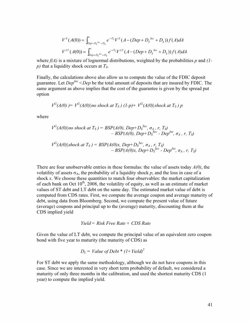
41

( (0)) ( ( )) ( )

( (0)) ( ( )) ( )

SSec

S S

SSec

S S

rTE E SecS SDep D D

rTLT LT SecS SDep D D

V A e V A Dep D D f A dA

V A e V A Dep D D f A dA

∞ −

+ +

∞ −

+ +

= − + +

= − + +

∫

∫

where f(A) is a mixture of lognormal distributions, weighted by the probabilities p and (1-p) that a liquidity shock occurs at TS. Finally, the calculations above also allow us to compute the value of the FDIC deposit guarantee. Let DepIns <Dep be the total amount of deposits that are insured by FDIC. The same argument as above implies that the cost of the guarantee is given by the spread put option

VG(A(0) )= VG(A(0)|no shock at TS ) (1-p)+ VG(A(0)|shock at TS ) p where

VG(A(0)|no shock at TS ) = BSP(A(0), Dep+DSSec, σA , r, TS)

– BSP(A(0), Dep+DSSec - DepIns, σA , r, TS)

VG(A(0)|shock at TS ) = BSP(A(0)x, Dep+DS

Sec, σA , r, TS) – BSP(A(0)x, Dep+DS

Sec - DepIns, σA , r, TS) There are four unobservable entries in these formulas: the value of assets today A(0), the volatility of assets σA, the probability of a liquidity shock p, and the loss in case of a shock x. We choose these quantities to match four observables: the market capitalization of each bank on Oct 10th, 2008, the volatility of equity, as well as an estimate of market values of ST debt and LT debt on the same day. The estimated market value of debt is computed from CDS rates. First, we compute the average coupon and average maturity of debt, using data from Bloomberg. Second, we compute the present value of future (average) coupons and principal up to the (average) maturity, discounting them at the CDS implied yield Yield = Risk Free Rate + CDS Rate Given the value of LT debt, we compute the principal value of an equivalent zero coupon bond with five year to maturity (the maturity of CDS) as

DL = Value of Debt * (1+Yield)5 For ST debt we apply the same methodology, although we do not have coupons in this case. Since we are interested in very short term probability of default, we considered a maturity of only three months in the calibration, and used the shortest maturity CDS (1 year) to compute the implied yield.

42

It is worth pointing out that the CDS implied yields under-estimates the true yield of bonds (see e.g. Longstaff et. all (2004)) and thus we over-estimate the value of debt in this case. We also computed the value of debt and implied transfers by treating the principal value as a zero coupon bond itself, thereby grossly under-estimating the value of debt. The transfers from equity holders to debt holders were very similar. For the calibration after the announcement, on 10/14/2008, we control for other confounding news between 10/10/2008 and 10/14/2008 by exploiting the estimation results in Sections 2.1 and 2.2, which provide the increase in the values of equity and debt that control for the market variation and the variation in GE capital, respectively. In particular, we impose that the values of equity and debt on 10/14/2008 are equal to the respective values at 10/10/2008 plus the adjusted values. Because these adjustments do not regard the value of short-term debt, we perform a similar adjustment to the 1-year CDS rates of banks on 10/14/2008, in which we control for the percentage decline in the CDS rate of GE capital. The remaining part of the calibration on 10/14/2008 is the same as at the previous date.

Appendix C. Taxpayers VAR Calculations For the Revised Paulson Plan, we compute the VaR from the perspective of tax payers as follows: First, we estimate the correlation structure of banks assets from the correlation of changes of short-term and long-term CDS rates. Second, we use these correlation structures to simulate the joint “liquidity shock” at TS as well as the joint assets realization at T=3. More specifically, we compute the liquidity shock at TS as follows: For each bank i, given a probability pi of a liquidity shock, we compute a cutoff level ei=N-1(pi), where N(.) denotes the cumulative standard normal distribution. We then simulate a vector ε~φ(0,R), where φ(0,R) denotes the multivariate normal density with correlation matrix R. A liquidity shock for bank i is declared if εi<ei . The correlation structure for liquidity shocks R is obtained from the variance covariance of the changes in short-term CDS rates. We simulate the value of assets A*(T) = ( A1

*(T),…, An*(T)) at T

jointly according to the model

log(A*(T)) | A(Ts) ~N(log(A*(Ts) + (μ-0.5 σA2)(T-TS) , ΣA(T-TS) )

where ΣA s the joint covariance matrix obtained from the correlation of CDS rate changes and the calibrated asset volatilities σA, and μ is the risk natural drift rate of assets, discussed further below. In this formula, for each bank i we have that its assets at TS are given by

Ai*(TS)=max(Ai(TS)+ DSi *1.25-(Depi+DSi+DSi

Sec),0)

To explain this formula, Ai(TS) denotes the amount of assets at TS, when the short term liabilities become “due”. This is given by Ai(TS)= xiAi(TS-) with a probability πi and Ai(TS)= Ai(TS-) with probability (1-πi), where πi denotes the risk natural probability of a shock, discussed below. To compute the 3-year VaR we need to take into account the

43

ability of banks to issue new debt, therefore we augment the asset value by the amount that the bank can issue at TS minus the total liabilities that become due at TS, according to the model, namely, deposits Dep, unsecured ST debt DS and secured ST debt DSi

Sec. If the bank total net assets at TS are smaller than 0, the bank fails. As before, we simulate the vector A(TS)=( A1(TS),…, An(TS)) jointly according to the model

log(A(TS)) ~N(log(A(0) + (μ0-0.5 σA2)TS , ΣATS )

where μ0 is the drift rate of assets before TS discussed further below. For each bank i we then compute the Government disbursement at T=3 as the difference between D – A(T), if any, where D equals the total LT debt maturing by T plus the new guaranteed debt DS*1.25 issued at TS, capitalized at the risk free rate to T (because it is government guaranteed), up to the maximum guarantee debt. To be conservative, we do not include “other liabilities” in D. On top of this, we compute the value of the investment in equity for the government, by using the Black and Scholes option pricing formula to compute the value of equity defined on the simulated assets at time T, minus of course the maturing guaranteed debt DS*1.25, capitalized at the risk free rate to T. This approach ensures the correct correlation between losses from the guarantee and equity investment, as if a bank needs a government intervention because of losses on assets, its equity value ought to small as well, implying a double loss for the government. The potential losses are given by the sum of losses from the guarantee and from the equity position. We compute the VaR for the other three cases (purchase of assets with and without overpayment, and pure capital infusion without guarantee) in an analogous manner. In particular consider the scenario in which the government purchases the banks’ assets (with or without overpayment). Let Ai(0) the amount purchased from bank i. We then simulate the value at T=3 of these assets Ai(T) as above. For symmetry, we consider the also in this case a shock at TS for the value of assets held by the government. In particular, we define the after-shock value of assets as Ai

*(Ts)= Ai(TS) if no shock occurs, and Ai

*(Ts)= xAi(TS) if a shock occurs. The remaining calculations are the same, noting that in this case there is no guarantee in place, and thus all of the VaR is coming from the devaluation of the assets purchased. Finally, for the case of a pure capital infusion we follow the same approach of simulating the value of assets at T=3. From the calibration we obtain the capital infusion necessary at 0 to yield a reduction in the value of CDS rates comparable to the ones in the data. From the capital infusion, we then obtain the percentage of government ownership of the bank and the value of initial assets of the bank (equal to old assets plus additional capital). We then simulate the value of assets at T as in the previous cases, taking into account that at TS the bank can fail if its assets are below the total amount of short term liabilities D. Recall that there is no guarantee in this case. At T, we compute the value of equity using the Black and Scholes formula for equity, and compute the profits/loss for the government as the difference from the initial capital infusion. We obtain the VaR number from the distribution of profits/losses at T.

44

One final important issue in the simulation of the asset value of each bank i, Ai(T), is how to move from the risk neutral dynamics to the risk natural (physical) dynamics, which is needed for VaR calculations. To move from risk neutral to risk natural probability measure, it suffices to make an assumption about the risk premium on traded assets. We assume that the market value of these assets has a relatively generous Sharpe ratio of 35%. Note that the higher the Sharpe ratio, the higher is the expected value of future assets and thus the lower is the VaR. Given the assumed Sharpe ratio λ=35%, the annual drift rate of assets after TS is then given by drift rate of assets = μ = risk free rate + λ σA where σA is the volatility of assets. This transformation must hold for t>TS. At TS there is also the liquidity shock, and thus the drift rate of assets before TS must be adjusted to ensure that the ex-ante Sharpe ratio is consistent with the possible crash. In particular, we proceed as follows: Let π denote the risk natural probability of a drop at TS. Then, we first require that the return on assets over TS must still be μ, that is E[A(TS)]=A(0) exp(μ TS), which in turn implies E[A(TS)] = (1- π)A(0)exp(μ0 TS)+ π x A(0) exp(μ0 TS)= A(0) exp(μ TS) or μ0(π )= μ - log((1- π) + π x)/TS That is, for given π we can compute the drift μ0 which ensures the proper expected return. We can then pin down π by imposing a Sharpe ratio also on the ex-ante investment. In particular, we can compute the variance of A(TS). The second moment is

E[A(TS)2]=[(1- π) + π x2] E[A(TS)2]= [(1- π) + π x2] E[A(TS)2] = [(1- π) + π x2]A(0)2exp((2μ0+σA

2)TS) yielding V(A(TS)) = E[A(TS)2]- E[A(TS)]2= = [(1- π) + π x2]A(0)2exp((2μ0+σA

2)TS) –[(1- π)+ π x]2 A(0)2 exp(2μ0 TS) = {[(1- π) + π x2]exp(σA

2 TS) –[(1- π)+ π x]2} A(0)2 exp(2μ0 TS) The TS Sharpe Ratio is then the expected excess return E[A(TS)/A(0)-exp(r TS)] divided by the standard deviation STD(A(TS)/A(0)) = V(A(TS)/A(0)) ½ , that is SR = E[A(TS)/A(0)-exp(r TS)] / STD(A(TS)/A(0))

= [(1- π) + π x –exp(-(μ0(π)-r) TS)]/ {[(1- π) + π x2]exp(σA2 TS) –[(1- π)+ π x]2}½

We obtain the probability π by imposing SR = 0.35 √TS. [In random walk-type of models, the Sharpe ratio is increases as a square root of time, as the expected return at the

45

numerator increases linearly, but the standard deviation increases as a square root of time].

46

References

Andrade Gregor and Steven N. Kaplan, 1998, “"How Costly Is Financial (Not Economic) Distress? Evidence from Highly Leveraged Transactions That Became Distressed." Journal of Finance, 1998, 53(5), pp. 1443-93.

Ballard, Charles L., Shoven, John B., Whalley, John, 1985 “General Equilibrium

Computations of the Marginal Welfare Costs of Taxes in the United States” The American Economic Review 75(1), 128 - 38.

Bebchuk, Lucian, 1988, "A New Approach to Corporate Reorganization," Harvard Law

Review, Vol. 101, pp. 775-804. Beals, Richard, 2009, “Warranted price” Breakingviews.com, 09 Jul 2009 Black, Fischer and Myron Scholes, 1973, "The Pricing of Options and Corporate

Liabilities". Journal of Political Economy 81 (3): 637–654. Chen, Hui, 2008, “Macroeconomic Conditions and the Puzzles of Credit Spreads and

Capital Structure," MIT Working Paper. Diamond, Douglas, Steve Kaplan, Anil Kasyap, Raghuram Rajan and Richard Thaler,

2008, “Fixing the Paulson Plan” WSJ.com, 26 September. Duffie, Darrell, 1999, "Credit Swap Valuation", Financial Analyst's Journal Duffie, Darrell, and Jun Liu, 2001, "Floating-Fixed Credit Spreads," Financial Analyst's

Journal Ivashina, Victoria and David Scharfstein, 2008, “Bank Lending Duirng the Financial

Crisis of 2008”, Harvard Business School Working Paper. Kroszner, R, 2003, "Is it Better to Forgive Than to Receive? An Empirical Analysis of

the Impact of Debt Repudiation," University of Chicago working paper. Landler, Mark and Eric Dash, 2008, “Drama Behind a $250 Billion Banking Deal”, New

York Times, October 15, 2008 Longstaff, Francis A, Sanjay Mithal and Eric Neis, 2004, "Corporate Yield Spreads:

Default Risk or Liquidity?", Journal of Finance. Merton, Robert C., 1974, "On the Pricing of Corporate Debt: The Risk Structure of

Interest Rates", Journal of Finance, Vol. 29, No. 2, (May 1974), pp. 449-470. Merton, Robert C., 1977, "An Analytic Derivation of the Cost of Deposit Insurance and

Loan Guarantees.", Journal of Banking and Finance, Vol. 1 , pp. 3-11.

47

Myers, S.C., 1977, “The Determinants of Corporate Borrowing", Journal of Financial

Economics, 5: 146-175. Philippon, T. and P. Schnabel, 2009, “Efficient Recapitalization”, working paper. Stiglitz, Joseph, 2008, "We Aren't Done Yet: Comments on the Financial Crisis and

Bailout," The Economists' Voice: Vol. 5: Iss. 5, Article 11. Swagel, Phillip 2009, "The Financial Crisis: An Inside View." Brookings Papers on Economic Activity VL, p.1-63. Zingales, Luigi, 2008a, "Why Paulson is Wrong," The Economists' Voice: Vol. 5: Iss. 5, Article 2. Zingales, Luigi, 2008b,"Plan B," The Economists' Voice: Vol. 5: Iss. 6, Article 4.

48

Figure 1: CDS Rates

All the rates are in basis points per year. Source: Datastream

0

200

400

600

800

1000

1200

1400

1600

10/10/2006 1/18/2007 4/28/2007 8/6/2007 11/14/2007 2/22/2008 6/1/2008 9/9/2008 12/18/2008

Citibank

Bank of America

JP Morgan

0

200

400

600

800

1000

1200

1400

1600

10/10/2006 1/18/2007 4/28/2007 8/6/2007 11/14/2007 2/22/2008 6/1/2008 9/9/2008 12/18/2008

Wachovia

Wells Fargo

General Electric

0

200

400

600

800

1000

1200

1400

1600

10/10/2006 1/18/2007 4/28/2007 8/6/2007 11/14/2007 2/22/2008 6/1/2008 9/9/2008 12/18/2008

Goldman Sachs

Morgan Stanley

Merrill Lynch

49

Figure 2: The Bank Run Index The figure plots the difference Rt = Pt(1) – Pt(2), where Pt(n) is the conditional probability of default in year n after t, conditional on not defaulting before n. These conditional probabilities are inferred from the term structure of CDS rates.

50

Figure 3: The Fear Index VIX This figure plots the CBOE VIX index, the expected risk neutral volatility obtained from short term options. The vertical dotted line corresponds to the 10/10/2008.

0

10

20

30

40

50

60

70

80

90

51

Figure 4: An Illustration of the Model Assets A(t) move over time. At TS there is the rollover of short term debt and deposits. However, at this time, there is also a probability p of a liquidity shock, which reduces the value of assets by x, that is, if the liquidity shock hits then A(TS)=x A(TS-). If at TS A(TS)<DS, there is default at TS. In this case, equity and long term debt holders are wiped out, while short term bond holders receive A(TS). If A(TS)>DS, assets A(t) evolve according to a lognormal model until TL. At TL, default occurs if A(TL)<DL. In the computations we further divide the short term debt in deposits and short term debt, while long term debt include also other liabilities.

No Default at TL Equity = A(TL) – DL LTDebt = DL

A(t)

Liquidity shock Payment at TS

DS = DL

TS TL

A(0) Default at TL Equity = 0 LTDebt = A(TL)

52

Figure 5: Predicting the size of the net value increase Figure 5A plots the net percentage value increase at the announcement of the plan on the run index, i.e. the difference in the probability of default embedded in the 1-year CDS rates and in the 3-year CDS rates before the announcement. Figure 5b plots the net percentage value increase at the announcement of the plan on the equity market performance of the corresponding stock during the crisis, i.e. from 7/1/07 to 10/10/08. 5A: % Net Increase in Enterprise Value on Probability of Run

Citi

BoA

JPM

Wac

WF

GS

MS

ML

-.02

0.0

2.0

4.0

6

0 5 10 15 index of probability of a run

% net increase in enterprise value Fitted values

53

5B: % Net Increase in Enterprise Value on Previous Stock Market Performance

Citi

BoA

JPM

Wac

WF

BNYMSS

GS

MS

ML

-.02

0.0

2.0

4.0

6

-1 -.8 -.6 -.4 -.2 0 stock market performance

% net increase in enterprise value Fitted values

FigurThis fimatchPaulso

re 6: Differefigure compareh the observed aon Plan (see Ta

5

6

7

ence in Equs the equity infadjusted reductable 3). All the

0

10

20

30

40

50

60

70

Citi

uity Infusionfusion under thtion in the CDS

e numbers are i

Bof

A

JPM

Paulson

n he Revised PauS rates observen billions of U

Wac

h

W.F

.

Plan Eq

ulson Plan and ed after the ann

US$.

Gol

dman

Mor

gan

uity Only

the equity infunouncement of

ML

5

usion needed tof the revised

54

o

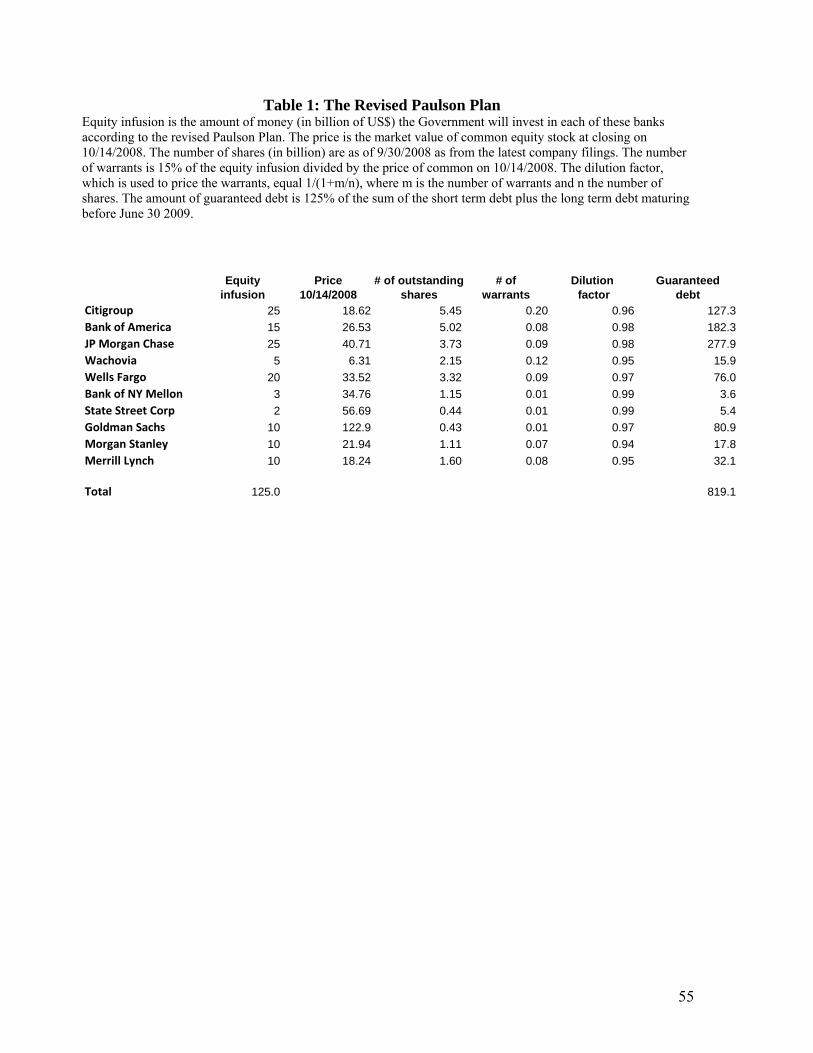
55

Table 1: The Revised Paulson Plan Equity infusion is the amount of money (in billion of US$) the Government will invest in each of these banks according to the revised Paulson Plan. The price is the market value of common equity stock at closing on 10/14/2008. The number of shares (in billion) are as of 9/30/2008 as from the latest company filings. The number of warrants is 15% of the equity infusion divided by the price of common on 10/14/2008. The dilution factor, which is used to price the warrants, equal 1/(1+m/n), where m is the number of warrants and n the number of shares. The amount of guaranteed debt is 125% of the sum of the short term debt plus the long term debt maturing before June 30 2009.

Equity Price # of outstanding # of Dilution Guaranteed

infusion 10/14/2008 shares warrants factor debtCitigroup 25 18.62 5.45 0.20 0.96 127.3Bank of America 15 26.53 5.02 0.08 0.98 182.3JP Morgan Chase 25 40.71 3.73 0.09 0.98 277.9Wachovia  5 6.31 2.15 0.12 0.95 15.9Wells Fargo 20 33.52 3.32 0.09 0.97 76.0Bank of NY Mellon 3 34.76 1.15 0.01 0.99 3.6State Street Corp 2 56.69 0.44 0.01 0.99 5.4Goldman Sachs  10 122.9 0.43 0.01 0.97 80.9Morgan Stanley  10 21.94 1.11 0.07 0.94 17.8Merrill Lynch 10 18.24 1.60 0.08 0.95 32.1

Total 125.0 819.1

                   

56

Table 2: Main Data on Banks Targeted by the Plan Panel A reports balance sheet information for the banks targeted by the first phase of the plan. The information comes from the banks’ 10Q filing as of 09/30/2008 (except Goldman Sachs and Morgan Stanley, whose data are as of 08/31/2008), which were the latest available on 10/10/2008. The data for the end of the third quarter are very similar. All figures in billions of US$. Panel B report some additional market information used in the analysis. Market capitalization is in billions of US$. The implied volatility is extracted from at-the-money call options on 10/10/2008 with the longest maturity available. Actual volatility is the annualized daily standard deviation of daily returns estimated during the period July-September 2008. The preferred yield is computed using the most recent preferred issue by each company that is trading. Dividend per share is obtained multiplying the last quarterly dividend times four.

Panel A: Balance Sheet data

Panel B: Other Market Information

Deposits Short Term Debt Long Non Interest Percent Term Other Total Total

Total Bearing Insured Total Unsecured Debt Liabilities Liabilities Equity AssetsCitigroup 780.3 108.0 47.4 352.3 101.9 396.1 395.7 1,924.4 126.1 2,050.5Bank of America 874.1 204.5 62.9 371.5 145.8 257.7 166.8 1,670.1 161.0 1,831.2JP Morgan Chase 969.8 203.0 37.4 446.4 222.3 255.4 434.0 2,105.6 145.8 2,251.0Wachovia  389.5 57.5 66.9 58.2 12.7 183.8 90.2 721.7 70.2 791.9Wells Fargo 339.1 89.4 64.2 86.1 60.8 103.9 31.9 561.1 48.0 609.1Bank of NY Mellon 174.2 81.7 3.1 20.3 2.9 15.5 30.0 240.0 27.5 267.5State Street Corp 150.9 70.0 0.6 100.2 4.3 4.1 17.3 272.5 13.1 285.6Goldman Sachs 29.1 0.0 14.3 443.5 64.7 176.4 387.2 1,036.2 45.6 1,081.8Morgan Stanley 36.8 0.0 81.6 193.7 14.2 202.3 518.8 951.6 34.5 986.1Merrill Lynch 90.0 0.0 85.3 242.9 25.7 232.5 272.0 837.4 38.4 875.8

Total 3,834 2,315 1,828 2,344 10,321 710 11,030

Mkt. Cap Implied Actual Preferred Dividends10/14/08 Volatility Volatility yields per share

Citigroup 101.5 77.59% 170.76% 12.46% 1.28Bank of America 133.1 77.75% 193.52% 8.83% 2.56JP Morgan Chase 151.7 57.37% 152.34% 8.84% 1.52

Wachovia  13.6 79.08% 696.48% 11.33% 0.20

Wells Fargo 111.3 56.48% 125.54% 8.73% 1.36Bank of NY Mellon 40.0 85.79% 177.78% 8.16% 0.96

State Street Corp 24.7 67.00% 166.84% 7.25% 0.96

Goldman Sachs (a) 52.6 67.73% 90.50% 7.79% 1.40

Morgan Stanley (a) 24.3 88.57% 151.25% 11.16% 1.08Merrill Lynch 29.2 82.23% 177.94% 11.55% 1.40

Average 68.2 73.96% 210.29% 9.61% 1.27Total 681.9

57

Table 3: Change in the Value of Long Term Debt around the Announcement of the Revised Paulson Plan CDS rates refer to a five year debt instrument and are expressed in basis points per year. The source is Bloomberg. The probability of default is calculated as (1- CDS rate/100)/(1- Recovery rate), where we assume the recovery rate to be 20%. The adjusted gain is the present value of the reduction in insurance costs paid on all the debt outstanding, with the actual structure of maturity, as a result of a drop in the CDS rates, adjusted for the percentage reduction in GE cost. As a discount rate we use 3.5%. The debt and the adjusted gain data are in billion of US$.

5 year 5 yearCDS spread CDS spread Raw Adjusted LT GE Adj. CDX Adj. Amount GE Adj. CDX Adj.

10/10/08 10/14/08 Decline Decline Debt Gain Gain Net Deriv. Gain Gain

Citigroup 341.7 144.6 197.1 72.9 396.1 21.4 23.9 103.4 3.6 3.9Bank of America 186.2 99.2 87.0 0.0 257.7 4.2 5.1 26.5 0.3 0.3JP Morgan 162.5 88.0 74.5 0.0 255.4 3.6 4.2 85.8 0.8 0.9Wachovia 267.5 109.2 158.3 34.1 183.8 7.5 8.4 13.4 0.4 0.4Wells Fargo 186.7 89.8 96.9 0.0 103.9 1.6 1.8 10.8 0.1 0.1Bank of NY Mellon 15.5 StateStreet 4.1 Goldman 540.0 201.7 338.3 214.1 176.4 17.6 19.0 103.9 6.7 7.1Morgan Stanley 1300.9 427.1 873.8 749.6 202.3 51.6 54.4 68.4 11.8 12.5Merrill Lynch 398.3 182.5 215.8 91.6 232.5 13.0 14.3 55.6 2.6 2.8

General Electric Capital 590.0 465.8 124.2 CDX Index 213.0 176.8 36.2

Total 1,828 120.5 131.3 467.8 26.3 28.0

Long Term Debt Net Derivative Payables

58

Table 4: Change in the Value of Equity around the Announcement of the Revised Paulson Plan Panel A refers to common equity, while Panel B to preferred equity. The market capitalization is price per share on 10/10/2008 times the number of shares outstanding. The betas are estimated from daily stock prices during the period 1/1/07-10/9/08. The daily prices are from Bloomberg. As a price for the preferred equity we use the most recently issued preferred of each company, assuming that all preferred of each bank have the same characteristics. The abnormal return equals raw return – beta * market return, where the market return (measures as S&P 500) increased by 11% over those two trading days. Value increase is the product of the initial market capitalization time the abnormal return. Market capitalizations and value increases are in billion of US$. Panel A: Common Equity

Panel B: Preferred Equity

Market cap Estimated Raw 10/10/2008 Beta return Beta =1 Est. beta Beta =1 Est. beta

Citigroup 76.89 1.97 0.32 0.21 0.10 16.1 7.9Bank of America 104.71 2.08 0.27 0.16 0.04 16.9 4.4JP Morgan Chase 155.19 1.77 -0.02 -0.13 -0.22 -20.5 -33.6Wachovia 11.07 4.28 0.23 0.12 -0.24 1.3 -2.7Wells Fargo 93.99 1.73 0.18 0.07 -0.01 7.0 -0.5Bank of NY Mellon 30.48 1.85 0.31 0.20 0.11 6.2 3.3State Street Corp 18.79 1.70 0.31 0.20 0.13 3.8 2.4Goldman Sachs 38.01 1.60 0.38 0.27 0.21 10.4 7.9Morgan Stanley 10.74 2.19 1.27 1.16 1.03 12.4 11.0Merrill Lynch 25.20 2.47 0.16 0.05 -0.11 1.2 -2.8

Total 565.1 54.8 -2.8Average 2.16 0.34 0.23 0.10

Abnormal return Value increase

Market cap Estimated Raw 10/10/2008 Beta return Beta =1 Est. beta Beta =1 Est. beta

Citigroup 9.48 1.35 0.37 0.26 0.22 2.4 2.1Bank of America 11.28 0.19 0.22 0.11 0.20 1.2 2.2JP Morgan Chase 5.32 0.45 0.12 0.01 0.07 0.0 0.4Wachovia 5.90 1.27 0.20 0.09 0.06 0.5 0.3Wells Fargo 0.34 0.36 0.22 0.11 0.18 0.0 0.1Bank of NY Mellon State Street Corp Goldman Sachs 0.74 0.50 0.21 0.10 0.15 0.1 0.1Morgan Stanley 0.30 1.14 1.13 1.02 1.01 0.3 0.3Merrill Lynch 4.50 1.03 0.39 0.28 0.28 1.3 1.2

Total 37.9 5.9 6.7Average 0.79 0.36 0.25 0.27

Abnormal return Value increase

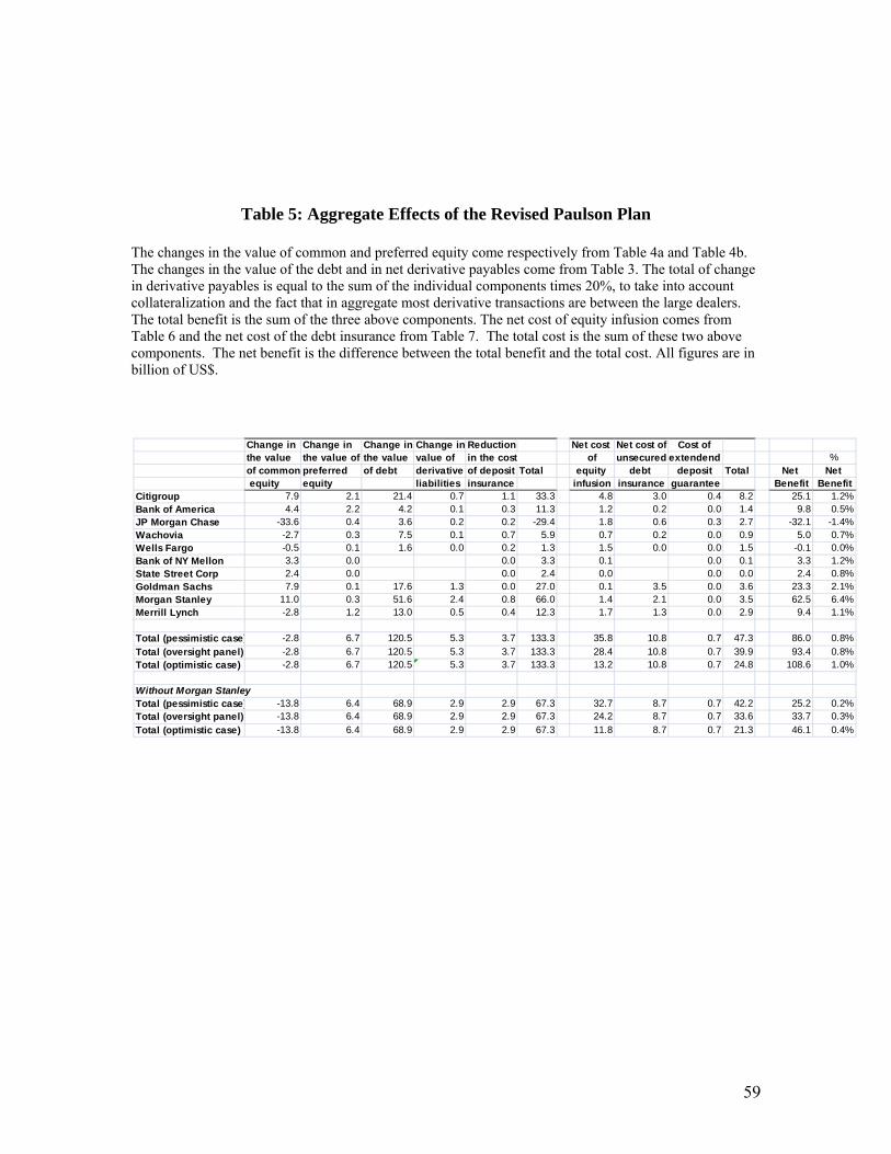
59

Table 5: Aggregate Effects of the Revised Paulson Plan

The changes in the value of common and preferred equity come respectively from Table 4a and Table 4b. The changes in the value of the debt and in net derivative payables come from Table 3. The total of change in derivative payables is equal to the sum of the individual components times 20%, to take into account collateralization and the fact that in aggregate most derivative transactions are between the large dealers. The total benefit is the sum of the three above components. The net cost of equity infusion comes from Table 6 and the net cost of the debt insurance from Table 7. The total cost is the sum of these two above components. The net benefit is the difference between the total benefit and the total cost. All figures are in billion of US$.

Change in Change in Change in Change in Reduction Net cost Net cost of Cost of the value the value of the value value of in the cost of unsecured extendend %of common preferred of debt derivative of deposit Total equity debt deposit Total Net Net equity equity liabilities insurance infusion insurance guarantee Benefit Benefit

Citigroup 7.9 2.1 21.4 0.7 1.1 33.3 4.8 3.0 0.4 8.2 25.1 1.2%Bank of America 4.4 2.2 4.2 0.1 0.3 11.3 1.2 0.2 0.0 1.4 9.8 0.5%JP Morgan Chase -33.6 0.4 3.6 0.2 0.2 -29.4 1.8 0.6 0.3 2.7 -32.1 -1.4%Wachovia -2.7 0.3 7.5 0.1 0.7 5.9 0.7 0.2 0.0 0.9 5.0 0.7%Wells Fargo -0.5 0.1 1.6 0.0 0.2 1.3 1.5 0.0 0.0 1.5 -0.1 0.0%Bank of NY Mellon 3.3 0.0 0.0 3.3 0.1 0.0 0.1 3.3 1.2%State Street Corp 2.4 0.0 0.0 2.4 0.0 0.0 0.0 2.4 0.8%Goldman Sachs 7.9 0.1 17.6 1.3 0.0 27.0 0.1 3.5 0.0 3.6 23.3 2.1%Morgan Stanley 11.0 0.3 51.6 2.4 0.8 66.0 1.4 2.1 0.0 3.5 62.5 6.4%Merrill Lynch -2.8 1.2 13.0 0.5 0.4 12.3 1.7 1.3 0.0 2.9 9.4 1.1%

Total (pessimistic case) -2.8 6.7 120.5 5.3 3.7 133.3 35.8 10.8 0.7 47.3 86.0 0.8%Total (oversight panel) -2.8 6.7 120.5 5.3 3.7 133.3 28.4 10.8 0.7 39.9 93.4 0.8%Total (optimistic case) -2.8 6.7 120.5 5.3 3.7 133.3 13.2 10.8 0.7 24.8 108.6 1.0%

Without Morgan Stanley Total (pessimistic case) -13.8 6.4 68.9 2.9 2.9 67.3 32.7 8.7 0.7 42.2 25.2 0.2%Total (oversight panel) -13.8 6.4 68.9 2.9 2.9 67.3 24.2 8.7 0.7 33.6 33.7 0.3%Total (optimistic case) -13.8 6.4 68.9 2.9 2.9 67.3 11.8 8.7 0.7 21.3 46.1 0.4%

60

Table 6: Shareholders’ Net Gain from the Government’s Equity Infusion This table provides two estimates of the present value of the claims the government is receiving in exchange for the equity infusion. In Panel A the present value of the preferred is computed using the yield to maturity of the bonds and the warrant is assumed to have a maturity of ten years. In Panel B the present value of the preferred is computed using the CAPM beta, while the warrant is assumed to have an effective maturity of 3 years since it is not protected against the payment of dividend after that date. Finally, the Congressional Oversight Report provided valuation of the same claims for all of our banks, except Merrill Lynch, Bank of NY Mellon and State Street. We impute their values using the average difference between our valuation the Report valuation for the common set of banks. In addition, Wachovia and Wells Fargo are reported jointly in the Report, and we split their values according to the equity infusion percentage in the second column. Panel A: Optimistic

Panel B: Pessimistic

Congr. Oversight Report Theoretical Theoretical Total TotalEquity Value of Value of Theoretical Difference Theoretical Infusion Preferred Warrant Value Claim Value Claim Difference

Citigroup 25 18.1 13.6 20.2 4.8 15.5 9.5Bank of America 15 12.7 7.4 13.8 1.2 12.5 2.5JP Morgan Chase 25 21.2 13.3 23.2 1.8 20.6 4.4Wachovia 5 3.8 3.3 4.3 0.7 4.6 0.4Wells Fargo 20 17.0 10.2 18.5 1.5 18.6 1.4Bank of NY Mellon 3 2.6 2.2 2.9 0.1 2.6 0.4State Street Corp 2 1.8 1.4 2.0 0.0 1.8 0.2Goldman Sachs 10 8.9 7.0 9.9 0.1 7.5 2.5Morgan Stanley 10 7.7 6.4 8.6 1.4 5.8 4.2Merrill Lynch 10 7.5 5.4 8.3 1.7 7.2 2.8

Total 125.0 101.3 70.0 111.8 13.2 96.6 28.4

Our calculations

Minimum between pessimistic Theoretical Theoretical Total and Congr. Oversight ReportEquity Value of Value of Theoretical DifferenceInfusion Preferred Warrant Value Claim Value Claim Difference

Citigroup 25 16.5 10.1 18.0 7.0 15.5 9.5Bank of America 15 9.6 5.8 10.5 4.5 10.5 4.5JP Morgan Chase 25 17.3 8.4 18.6 6.4 18.6 6.4Wachovia 5 1.9 2.2 2.2 2.8 2.2 2.8Wells Fargo 20 14.0 6.5 15.0 5.0 15.0 5.0Bank of NY Mellon 3 2.0 1.5 2.3 0.7 2.3 0.7State Street Corp 2 1.4 0.8 1.5 0.5 1.5 0.5Goldman Sachs 10 7.2 4.3 7.9 2.1 7.5 2.5Morgan Stanley 10 6.2 4.7 6.9 3.1 5.8 4.2Merrill Lynch 10 5.8 4.1 6.4 3.6 6.4 3.6

Total 125.0 81.9 48.4 89.2 35.8 85.3 39.7

Our calculations

61

Table 7: Cost of the Bank Debt Guarantee Provided by the FDIC

The CDS rates, in basis points, are for a three year contract and are obtained from Datastream. All the balance sheet information is as of 09/30/08, apart from Goldman Sachs and Merrill Lynch whose values are as of 08/31/08. The total debt guaranteed is 125% of the short term unsecured debt. The total cost of the Government guarantee is discounted value of the difference between the value of this guarantee (CDS rate times the value of the debt guaranteed) minus the cost to the banks (75 basis points times the value of the debt guarantee) over the period of the guarantee (the next three years). All values in billions of US$, exception made for the CDS rates.

Debt Insurance Deposit InsuranceUnsecured 3-year CDS Total Total Uninsured Total SavingsShort term spread Guaranteed Cost of Non-Int. bearing Cost of from Deposit

Debt 10/14/2008 debt Insurance Deposits Insurance GuaranteeCitigroup 101.9 155.9 127.3 3.0 56.8 0.39 1.1

Bank of America 145.8 79.1 182.3 0.2 75.9 0.03 0.3

JP Morgan Chase 222.3 82.3 277.9 0.6 127.1 0.28 0.2

Wachovia  12.7 117.3 15.9 0.2 19.1 0.00 0.7

Wells Fargo 60.8 74.1 76.0 0.0 32.1 0.00 0.2

Bank of NY Mellon 2.9 3.6

State Street Corp 4.3 5.4

Goldman Sachs 64.7 227.7 80.9 3.5 0.0 0.00 0.0

Morgan Stanley 14.2 490.3 17.8 2.1 0.0 0.00 0.8

Merrill Lynch 25.7 213.5 32.1 1.3 0.0 0.00 0.4

Total 655.3 819.1 10.8 310.8 0.7 3.7

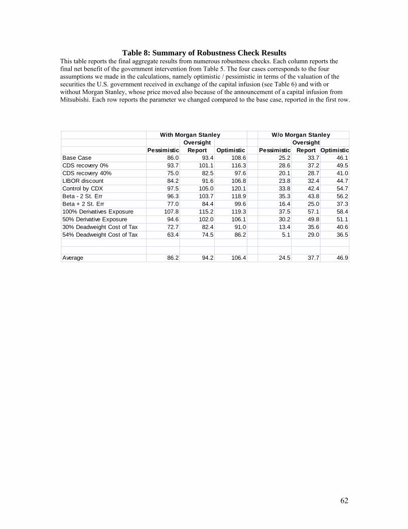
62

Table 8: Summary of Robustness Check Results This table reports the final aggregate results from numerous robustness checks. Each column reports the final net benefit of the government intervention from Table 5. The four cases corresponds to the four assumptions we made in the calculations, namely optimistic / pessimistic in terms of the valuation of the securities the U.S. government received in exchange of the capital infusion (see Table 6) and with or without Morgan Stanley, whose price moved also because of the announcement of a capital infusion from Mitsubishi. Each row reports the parameter we changed compared to the base case, reported in the first row.

With Morgan Stanley W/o Morgan StanleyOversight Oversight

Pessimistic Report Optimistic Pessimistic Report OptimisticBase Case 86.0 93.4 108.6 25.2 33.7 46.1CDS recovery 0% 93.7 101.1 116.3 28.6 37.2 49.5CDS recovery 40% 75.0 82.5 97.6 20.1 28.7 41.0LIBOR discount 84.2 91.6 106.8 23.8 32.4 44.7Control by CDX 97.5 105.0 120.1 33.8 42.4 54.7Beta - 2 St. Err 96.3 103.7 118.9 35.3 43.8 56.2Beta + 2 St. Err 77.0 84.4 99.6 16.4 25.0 37.3100% Derivatives Exposure 107.8 115.2 119.3 37.5 57.1 58.450% Derivative Exposure 94.6 102.0 106.1 30.2 49.8 51.130% Deadweight Cost of Tax 72.7 82.4 91.0 13.4 35.6 40.654% Deadweight Cost of Tax 63.4 74.5 86.2 5.1 29.0 36.5

Average 86.2 94.2 106.4 24.5 37.7 46.9

63

Table 9: Implied Estimates of the Cost of Bankruptcy This table estimates the value of bankruptcy costs implicit in the market response to the Paulson Plan. The first two columns report the total enterprise value (book value of debt and preferred plus market value of common equity) and the change in the market value of each of the banks involved in the Paulson Plan (all values are in billions of US$). The third and fourth columns report the risk neutral probability of bankruptcy embedded in the CDS rates before and after the announcement. Columns five and six report the implicit estimate of the bankruptcy costs calculated according to formula (8) in the text.

Enterprise Change in Prob of Prob of Estimated EstimatedValue Enterprise default default Bankrupcty Bankrupcty

Value 10‐Oct 14‐Oct Costs bn $ Costs %Citigroup 2,026 25 5.08 2.16 147 7.3%Bank of America 1,803 10 1.43 0.76 100 5.5%JP Morgan 2,257 -32 1.42 0.77Wachovia 735 5 4.05 1.66 34 4.6%Wells Fargo 672 0 1.45 0.69Bank of NY Mellon 280 3 StateStreet 297 2 Goldman 1,089 23 9.74 3.72 93 8.5%Morgan Stanley 976 62 30.33 8.26 162 16.6%Merrill Lynch 867 9 7.69 3.26 65 7.5%

Total 11,002 recovery rate 0.2discount rate 0.1

64

Table 10: Value Transferred to Long Term Debt by Equity Infusion This table estimates the changes in the value of equity due only to the infusion of equity. The first two columns report the value in the model of long term debt and equity before the equity infusion, columns 3 and 4 report the value of long term debt and equity after the equity infusion reported in column 5. Columns 6 and 7 report the difference in the value of debt and equity as a result of the equity infusion. The last column reports what fraction of the equity infusion goes to increase the value of the long term debt. All values in billions of US$, exception made for the fraction of equity infusion to debt.

Enterprise Change in Prob of Prob of Estimated EstimatedValue Enterprise default default Bankrupcty Bankrupcty

Value 10‐Oct 14‐Oct Costs bn $ Costs %Citigroup 2,026 25 5.08 2.16 147 7.3%Bank of America 1,803 10 1.43 0.76 100 5.5%JP Morgan 2,257 -32 1.42 0.77Wachovia 735 5 4.05 1.66 34 4.6%Wells Fargo 672 0 1.45 0.69Bank of NY Mellon 280 3 StateStreet 297 2 Goldman 1,089 23 9.74 3.72 93 8.5%Morgan Stanley 976 62 30.33 8.26 162 16.6%Merrill Lynch 867 9 7.69 3.26 65 7.5%

Total 11,002 recovery rate 0.2discount rate 0.1

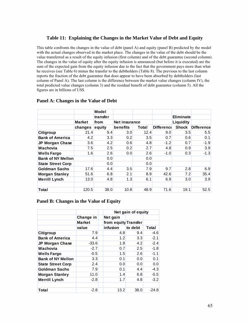
65

Table 11: Explaining the Changes in the Market Value of Debt and Equity

This table confronts the changes in the value of debt (panel A) and equity (panel B) predicted by the model with the actual changes observed in the market place. The changes in the value of the debt should be the value transferred as a result of the equity infusion (first column) and of the debt guarantee (second column). The changes in the value of equity after the equity infusion is announced (but before it is executed) are the sum of the expected gain from the equity infusion due to the fact that the government pays more than what he receives (see Table 6) minus the transfer to the debtholders (Table 8). The previous to the last column reports the fraction of the debt guarantee that does appear to have been absorbed by debtholders (last column of Panel A). The last column is the difference between the market value changes (column IV), the total predicted value changes (column 3) and the residual benefit of debt guarantee (column 5). All the figures are in billions of US$.

Panel A: Changes in the Value of Debt

Panel B: Changes in the Value of Equity

Modeltransfer Eliminate

Market from Net insurance Liquidity changes equity benefits Total Difference Shock Difference

Citigroup 21.4 9.4 3.0 12.4 9.0 3.5 5.5Bank of America 4.2 3.3 0.2 3.5 0.7 0.6 0.1JP Morgan Chase 3.6 4.2 0.6 4.8 -1.2 0.7 -1.9Wachovia 7.5 2.5 0.2 2.7 4.8 0.9 3.9Wells Fargo 1.6 2.6 0.0 2.6 -1.0 0.3 -1.3Bank of NY Mellon 0.0 0.0 State Street Corp 0.0 0.0 Goldman Sachs 17.6 4.4 3.5 7.9 9.7 2.8 6.9Morgan Stanley 51.6 6.8 2.1 8.9 42.6 7.2 35.4Merrill Lynch 13.0 4.8 1.3 6.1 6.9 3.0 3.9

Total 120.5 38.0 10.8 48.9 71.6 19.1 52.5

Change in Net gain Market from equity Transfervalue infusion to debt Total

Citigroup 7.9 4.8 9.4 -4.6Bank of America 4.4 1.2 3.3 -2.1JP Morgan Chase -33.6 1.8 4.2 -2.4Wachovia -2.7 0.7 2.5 -1.8Wells Fargo -0.5 1.5 2.6 -1.1Bank of NY Mellon 3.3 0.1 0.0 0.1State Street Corp 2.4 0.0 0.0 0.0Goldman Sachs 7.9 0.1 4.4 -4.3Morgan Stanley 11.0 1.4 6.8 -5.5Merrill Lynch -2.8 1.7 4.8 -3.2

Total -2.8 13.2 38.0 -24.8

Net gain of equity

66

Table 12: Change in the value of assets implied by the model In the extended Merton (1974) model described in Appendix B, we choose the four unobservable variables (value of assets today A(0), volatility of assets σA, probability of a liquidity shock p, and loss in case of a shock x) to match the four observables: the market capitalization of each bank, the volatility of equity, the estimated of market value of ST debt, and the estimated market value of LT debt. The estimated market value of debt is computed from CDS rates. The first four columns report the value estimated by using the October 10, 2008 data, while the second four columns the value estimated by using the October 14, 2008 data. The previous to the last column report the difference between the value of assets estimated the two days and the last column reports the change in the value of assets as derived in Table 5 (common equity, preferred equity, debt). All the $ figures are in billions of US $. The volatilities and the probabilities are in percentage terms. The recovery rate is the fraction of value recovered.

Estimated Actual Asset Asset Prob of Recovery Asset Asset Prob of Recovery changes in changes in Volatility Value run Rate Volatility Value run Rate asset value asset value

Citigroup 9.5 1,915 1.00 0.25 8.8 1,945 0.69 0.29 29.8 31.4Bank of America 11.4 1,748 0.27 0.31 11.3 1,758 0.21 0.31 10.5 10.9JP Morgan Chase 9.3 2,202 0.28 0.30 7.7 2,172 0.22 0.31 -30.0 -29.7Wachovia 7.3 708 0.54 0.27 5.8 713 0.31 0.33 4.6 5.1Wells Fargo 20.1 651 0.28 0.27 19.2 652 0.21 0.27 0.9 1.1Bank of NY Mellon State Street Corp Goldman Sachs 8.0 999 1.91 0.23 7.2 1,024 1.25 0.26 24.6 25.6Morgan Stanley 7.0 825 5.71 0.15 5.3 887 3.17 0.16 62.3 62.9Merrill Lynch 7.8 803 1.50 0.24 6.2 813 1.04 0.28 10.3 11.4

Average 10.1 1.4 0.3 8.9 0.9 0.3Total 9,851 9,964 113 119

Values estimated on 10/10/2008 Values estimated on 10/14/2008

67

Table 13: Cost of Alternative Plans This table measures the Revised Paulson Plan along four dimensions and compares it along these dimensions with four alternatives. The four dimensions are: the amount of funds required by the plan, the ex ante cost of the plan for taxpayers, the value at risk for taxpayers (5% probability of a loss in three years), and the percentage of ownership the Government would have acquired if it invested in straight equity. All the plans in Panel A are constrained to deliver a reduction in CDS rates at least as big as the adjusted decline reported in Table 3. All the plans in Panel B are constrained to deliver a reduction in CDS rates at least as big as the raw decline reported in Table 3. All the figures are in billions of US$. Panel A: Target = adjusted reduction in CDS rates

Panel B: Target = raw reduction in CDS rates

Revised Pure Long-termPaulson Equity Debt

Plan no over 20% over Infusion for Equitypayment payment Swap

Investment required 125 3,084 953 261 0

Net cost to taxpayers 49 0 191 65 0

5% 3 year Value at Risk 98 127 49 211 0

% of banks owned by Government 20% 0 0 40% 0

Original Paulson Plan:Asset Purchase

Revised Pure Long-termPaulson Equity Debt

Plan no over 20% over Infusion for Equitypayment payment Swap

Investment required 125 4,585 1,654 495 0

Net cost to taxpayers 49 0 331 139 0

5% 3 year Value at Risk 93 203 88 363 0

% of banks owned by Government 20% 0 0 52% 0

Original Paulson Plan:Asset Purchase