Paul Woodward Sept. 30, 2001...Running the 2-D Wind Tunnel Program Paul Woodward Sept. 30, 2001 The...

Running the 2-D Wind Tunnel Program Paul Woodward Sept. 30, 2001

The 2-D wind tunnel simulator program builds on the experience you gained playing with the shock tube experiment simulator program Gas1D. That earlier program simulated the behavior of gas confined to a thin tube, describing only the variations in the gas density, pressure, and velocity that result in the direction along the tube. The wind tunnel program also considers the behavior of gas flowing in a duct, but now the variations in the gas state across the width of the duct are described along with the variations along the duct’s length. However, these wind tunnel flows are still simplified from their real life counterparts. We simplify them by assuming that there are no variations in the state of the gas in the third dimension. This third dimension is the direction that points out of the paper when we draw pictures of the flow with the duct length as the horizontal axis and the duct width as the vertical one.

2-D flows in nature: Believe it or not, fluid flows that are well approximated by 2-D models like this do exist in

nature. Perhaps the most familiar example is the large-scale weather. No one complains that weather maps in the newspaper are 2-D drawings, showing only variations in air temperature, for example, in the north-south and east-west directions. There is of course strong local variation in the vertical direction, as is obvious if you simply step outside and have a look at the weather. However, these vertical variations tend to be roughly the same at each horizontal location. They are caused mainly by the changes in air pressure, temperature, and density that come from the atmosphere’s confinement to the earth by the earth’s gravity. Anyone who has climbed a high mountain knows that the air gets cooler at higher altitudes. If you climb really high, you also know that the air gets thinner. But these vertical variations are about the same everywhere. It doesn’t matter where you put a mountain, the air at its top will always be cooler and thinner. The

LCSE PPM Wind Tunnel Simulator User’s Guide 9/30/2001

2

variations in the atmosphere that most obviously drive weather, at least here in the upper Midwest, come from the horizontal winds, which bring regions of different temperature air to us from some other location. This is of course a largely two-dimensional effect. Thus 2-D weather maps contain most of the information we need.

Experimental set-up: The experimental situation simulated in the wind tunnel program is the flow of air from left

to right down the length of a duct, or wind tunnel, which contains a step. The walls of the duct, including the step, are impenetrable and unmovable, by assumption. We can think of them as constructed of very thick steel. But perhaps steel is not the right material for us to imagine, because we will also assume that the walls of our wind tunnel do not conduct heat at all. In the simulation, the temperature of the air will be entirely unaffected if it is located next to one of these walls. You can imagine that the wind tunnel is made of some thermally insulating material, like wood or plastic, so that it does not affect the air temperature near it. Alternatively, if you prefer, you can imagine that the wind tunnel is very large. Then the large size of the wind tunnel would limit any effects of thermal conduction to a thin layer of gas right next to the walls. If the wind tunnel were large enough, that layer would be so small that we could simply ignore its existence in our simulator program. This second way of looking at the experiment is the better one, since real wind tunnels are usually made of steel, a good thermal conductor, but they are usually large enough that only very thin layers of gas near the walls are affected by heat transfer to or from these walls.

The idea of the experiment we will simulate is that air flows in from the left end of our wind tunnel at a velocity that we will prescribe. The air strikes the step in the wind tunnel and flows around it. This creates a bow wave, and the bow wave will reflect off of the opposite wall of the tunnel. You can get a better idea of this set-up by looking at the form painted on your computer screen by the program. This form is shown at the top of the next page. You can see the wind tunnel’s experiment section in the picture box on the center of the form. In this snap shot of the


3

form, which appears when you start up the program, the density of the air in the wind tunnel is displayed in shades of gray. White is the highest density, and black is the lowest. The step in the wind tunnel here appears black. Just as in the Gas1D program, you can select any of a number of different variables to display which characterize different aspects of the air flow in the wind tunnel. As in that program, the minimum and maximum values in the display window, which are mapped to the black and white levels, respectively, are displayed in the two text boxes below the picture box. To the left of the minimum value’s text box is another which gives the time at which the snap shot shown in the picture box was taken. (It is 0 here, since the flow has not yet started.)

Just for fun, the flow is initialized with a smooth density variation in the air inside the wind tunnel. This will give you something interesting to look at as the flow develops. Another aspect


4

of the initial flow that makes its subsequent development more interesting is a shear layer that is introduced part of the way up from the bottom wall. You can see this if you select the x-velocity for display. Then you see the picture at the top of this page. Since white represents the largest x-velocity (2.123, according to the text box below the picture), we know that the air in the upper part of the wind tunnel is moving more rapidly to the right than that below it. The minimum air velocity shown in 0, which is the velocity that the program sets in the grid cells inside the immovable step in the wind tunnel.

The velocity in the lower section of air in the tunnel is given in the text box above the picture that is located to the left of the label “Mach Number.” This text box indicates that the air in the lower portion of the wind tunnel is moving to the right at Mach 2, that is, at twice its speed of sound. The flow is initialized in such a way that the sound speed in this air is exactly 1. Thus


5

its x-velocity is 2. As the experiment proceeds, air will be injected at the left-hand boundary at Mach 2 in the lower portion of the wind tunnel, and it will be injected at the velocity 2.123 in the upper portion of the tunnel. If you select for display the y-velocity, you will see that this is zero everywhere in the wind tunnel. As the air must flow around the step in the tunnel, however, this vertical velocity component will become non-zero in that region.

How to specify the names and locations of disk files generated by the program: In discussing the experimental set-up in the

section above, we have jumped ahead of ourselves slightly. When you start up the program, you are first forced to let the program know where it should write disk files that it needs for its work. A message box, shown at the right, pops up on your screen to explain this process to you. You must press the “OK” button in order to proceed. Immediately thereafter, as advertised, the program will prompt you for the directory to use for these files and the “stem name” to which it will append suffixes for individual working files. It will prompt you for this information by bringing up a standard file system browser window, whose use should be familiar to you from various Microsoft Windows products, like WORD or PowerPoint.

This file system browser window is shown here at the right. By default, it places you initially in the directory from which you launched the wind tunnel simulator program. Also by default, it supplies you with a suggested stem name for the disk files that the program will automatically generate and write into this directory (or into the directory that you specify by manipulating the browser window to point elsewhere than its default location). This


6

default stem name is “WindTunnel.” This stem name can be modified, so that you can keep on your hard disk files from one successful experiment without overwriting them with the files from a subsequent experiment. While you are playing around with this program, however, you will probably find it convenient to simply use the default directory and file name stem. This way each experiment will overwrite the results of the previous one, so that your disk does not become clogged. It is also very easy to specify these defaults, because all you have to do is simply press the “Enter” key on your keyboard each time one of these little windows pops up.

How to alter the location and strength of the shear layer in the wind tunnel: Of course it is simplest to accept the default values

for the shear layer in the wind tunnel, but if you would like to change them, the program allows you to do so. To do this, you must click on the button labeled “Advanced Setup,” which is located on the form just to the left of the big, red “Pause” button above the picture box. An input box will pop up, which is shown here at the right. It prompts you for the vertical location of this shear layer, measured in grid cells. The present value is given as the default, so that if you just press your “Enter” key, this vertical location will not be altered. In the example shown, the number of grid cells with the lower flow-in parameters is 38. This measure of vertical location is to be interpreted in terms of the total number of grid cells in the vertical direction across the entire wind tunnel width. That number is given in the text box just to the left of the label “N Y-Grid Cells” at the top of the form. In the case shown here, that number is 64. Therefore the shear layer is located 38/64 of the way up from the bottom wall.

To change the jump in density across the shear layer, you can type in a new value in the input box that pops up after you have made your decision on the shear layer vertical position. This new input box is shown at the right here. The present value of the air density in the upper region of the flow is given as a default. Once again, to leave this value unchanged, you can simply press


7

your “Enter” key. In the case shown, this default density is 1.5. This value is to be compared to 1, the built-in value of the density of the air that will be injected below the shear layer location. To have no change in the density across the shear layer, you can type in 1 at this prompt. Note that the label of this input box talks about a “contact discontinuity” rather than a shear layer. Don’t worry about this. Technically, a contact discontinuity is just a surface at which the density of a gas changes suddenly, but the pressure does not change. There can be shear at such a contact discontinuity, or there might not be shear there. By saying that this density jump is a contact discontinuity, the wind tunnel program is telling you that the pressure on each side, in the injected air, will be the same. This feature is built into the program. You cannot set the pressure of the injected air. It is determined from the joint requirements that the density in the region below the shear layer (or contact discontinuity) must be 1 and the sound speed in this region must also be 1.

You can change the jump in velocity across the shear layer by entering a new value in the input box that pops up after you have prescribed the density above the shear layer. This new input box is shown at the right. If you want to eliminate the shear at this contact discontinuity, you can type in the same velocity value that is shown in the text box just to the left of the label “Mach Number.” Because the sound speed in the incoming gas below the shear layer is 1, the velocity of this gas is also its Mach number. Thus in this example, typing in a value of 2 in this text box would eliminate the shear at this inflowing contact discontinuity.

How to alter the height and horizontal position of the step in the wind tunnel: The height and horizontal position of the step in the wind tunnel are easily altered by

entering new values for these parameters in the appropriate text boxes at the top of the form. These parameters of the experiment are measured in terms of grid cells. The wind tunnel section that is simulated is always twice as long as it is wide. Thus the value displayed in the text box to the left of the label “N X-Grid Cells” is always exactly twice the value displayed in the text box to the left


8

of the label “N Y-Grid Cells” near the top-left corner of the form. You can change either of these numbers in order to coarsen the grid resolution, so that the experiment will run faster on your computer, or to refine the grid resolution, so that the computed results will more closely simulate real gas behavior. Whenever you change one of these numbers, the other is automatically adjusted as well in order to keep the grid cells square and the wind tunnel length exactly twice the wind tunnel width.

The height of the step in the wind tunnel, measured in grid cells, is displayed in the text box to the left of the label “N Step Height” near the top center of the form. You can change this number to any desired value, although if you type in too large a value, an input box will pop up showing you the maximum step height that is allowed for the number of grid cells that you have specified across the wind tunnel width. The horizontal position of the wind tunnel step is displayed in the text box to the left of the label “N Before Step” on the form. In this text box you may enter any desired number of grid cells that you would like to have between the left-hand boundary and the front of the step in your wind tunnel. Once again, if you type in a value that lies outside the bounds allowed by the program, an input box will pop up which has that bound as a default value.

How to change the in-flow Mach number: As you have seen already, the speed of the inflowing air in the region below the shear layer

is displayed in the text box to the left of the label “Mach Number.” The Mach number of this gas and its speed are the same, since this gas has a sound speed of 1 by construction. You may enter any desired Mach number value in this text box. If you enter a value less than 1, the inflow will be subsonic, and sound waves will be able to propagate up the wind tunnel’s length to the inflow edge at the left. When sound signals reach this in-flow boundary, they will not be treated correctly there. Therefore, the operation of the program is correct only for supersonic in-flow speeds, or in-flow Mach numbers greater than 1.


9

You will notice that below the Mach number text box is a text box labeled “Gamma.” The value displayed in this text box is 1.4. This parameter characterizes the relationship between pressure, density, and temperature in the gas in the wind tunnel. It is only of interest to experts. You are best advised not to change this parameter.

How to set the duration and output snap-shot frequency for your experiment: Before you run a wind tunnel experiment, you need to set the parameters that will determine

what and how much output will be generated. As in the Gas1D program, time is measured in special units specific to your wind tunnel. The sound speed in the inflowing gas below the shear layer is always set to 1. The width of the wind tunnel is also assumed to be 1. These facts determine an appropriate measure of time, in units of the time that it takes sound, traveling at the sound speed in the gas below the shear layer, to cross the wind tunnel’s width. Because the wind tunnel is always twice as long as it is wide, gas traveling at Mach 2 will traverse the length of the wind tunnel in one of these time units.

The units that the program uses for your experiment are as follows. Lengths are measured in wind tunnel widths, speeds are measured in multiples of the sound speed of the gas entering the tunnel at the lower left, densities are measured in units of the density of this entering gas, and times are measured in multiples of the time interval required for sound in this gas to travel a distance equal to the wind tunnel width. Thus, alternatively stated, the width of our wind tunnel is 1, the density and sound speed in the gas entering it at the lower left is 1, and the time for sound to travel one length unit in this entering gas is also 1.

Just as in the Gas1D experiments, we can use this very convenient system of units because the behavior of the gas does not depend upon the units that we use to describe it, nor does it depend upon the actual size of our wind tunnel, so long as this is sufficiently large to justify our assumption that any special layers of gas along the wind tunnel walls can be ignored. If we say that the


10

wind tunnel is one mile across rather than one foot across, then the time that it will take for the flow to develop will be 5280 times longer, but the flow will develop in precisely the same fashion.

Now that you understand the units we use for the wind tunnel experiment, you can choose how long you want the experiment to run. If you run it for only one time unit, sound signals will only have time to traverse the wind tunnel width once. This is time enough for these sound signals to push the gas in the upper portion toward the upper wall, so that the gas in the lower portion can flow around the step, but it is not enough time for that upper gas to push back and help, by means of sending reflected sound signals, to establish a more steady flow in the wind tunnel.

As a general rule of thumb, something significant will happen to your flow in one time unit, but it will take about 4 time units for the flow to adjust after you start it up in the artificial state that the program sets up. At the outset of your experiment, the gas will be flowing everywhere directly to the right, and there will be no disturbances present. Immediately upon starting the flow simulation, the gas will crash into the step in the wind tunnel and begin to force its way around it. This process is fun to watch, and it will take about one time unit. But it is usually a good idea to run your simulation for at least 4 time units in order to see how things ultimately shape up.

Depending upon how long you choose to run your experiment, you may select a number of snap shots of the flow per time unit that you want to save on your hard disk in order to review the flow development after your experiment is completed (or during any time when you choose to pause the flow simulation’s execution by clicking on the “Pause” button). Be aware that each flow snap shot is a bitmap file consisting of 3 bytes per pixel of your screen in the region of the picture box on the program’s form. Depending upon the resolution of your screen, this might vary from 1/3 MB to 2/3 MB. Saving a thousand such bitmap files could run into significant space on your hard drive.

The flow snap shots that you save can be reviewed from the program form by manipulating the vertical scroll bar just to the left of the picture box on the form. You can also move forward or


11

back one snap shot by using your arrow keys once this vertical scroll bar is activated. To save any display that you particularly like, together with the form that shows the experiment’s parameter values, you can simply press Alt-PrntScrn on your keyboard while the program window is active. A bitmap image of the form is then place on the clipboard, from which you can paste it into a WORD document, a PowerPoint presentation, or a Paint file for sharing with another student or with your instructor.

If you are just playing around with the wind tunnel simulator and do not wish to review stored snap shots of your flows, then you can specify that only, say, 1 snap shot per time unit be saved. You will still see the entire flow development as a movie as it is computed on your PC, but after the run is finished, you will not be able to review the flow development without running the experiment over again.

How to run a wind tunnel experiment: Why don’t you run an experiment now? Since it is so easy, why not just accept all the

defaults and just run whatever has been set up for you with no effort on your part. Just fire up the wind tunnel simulator by double clicking on the executable file “PPM2Dgui.exe” or “PPM2DguiSmallForm.exe” and press enter each time a text input box pops up on your screen. Be careful to have disk space available in the directory where you have placed the program executable file. If you do not have disk space, then you should reset the “Plots Per Period” to a small number, like 1. After pressing “Enter” when the first two input boxes pop up, you are ready to begin, unless you need to reset the amount of output, run duration, or whatever you choose. To start the simulation, just click on the big green “Begin” button near the right top of the form, or simply press “Enter.” You will have to press “Enter” 4 more times, as input boxes pop up, but that’s easy. Then you should be off and running. You should see a real-time movie of the density distribution in your wind tunnel as your flow develops.


12

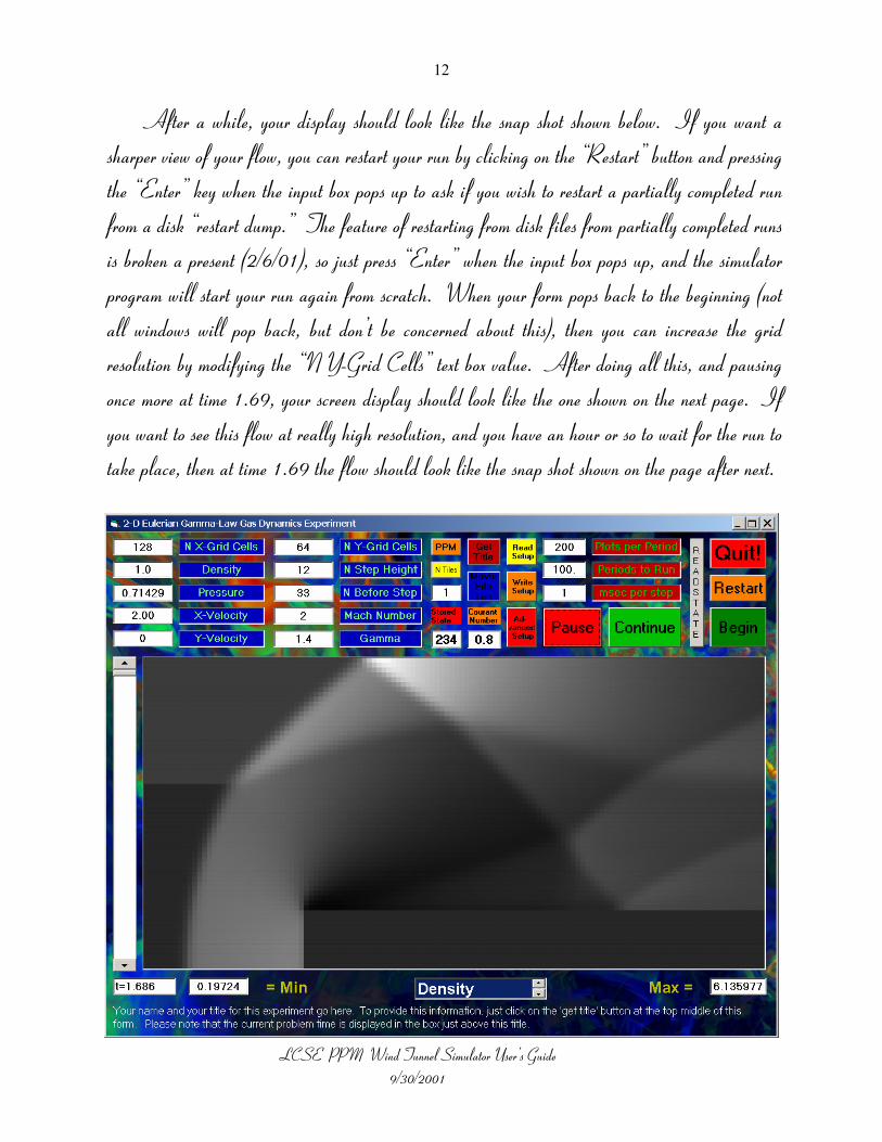
After a while, your display should look like the snap shot shown below. If you want a sharper view of your flow, you can restart your run by clicking on the “Restart” button and pressing the “Enter” key when the input box pops up to ask if you wish to restart a partially completed run from a disk “restart dump.” The feature of restarting from disk files from partially completed runs is broken a present (2/6/01), so just press “Enter” when the input box pops up, and the simulator program will start your run again from scratch. When your form pops back to the beginning (not all windows will pop back, but don’t be concerned about this), then you can increase the grid resolution by modifying the “N Y-Grid Cells” text box value. After doing all this, and pausing once more at time 1.69, your screen display should look like the one shown on the next page. If you want to see this flow at really high resolution, and you have an hour or so to wait for the run to take place, then at time 1.69 the flow should look like the snap shot shown on the page after next.


13

In this sequence of results computed at different grid resolutions, you can see the picture of the flow appear to come into focus. The more grid cells you use in the simulation, the more closely your results will approximate the flow of air you would see in a real 2-D wind tunnel (but you should be aware that there are no real 2-D wind tunnels, only real 3-D ones). We will use the most accurate of the flows shown here to illustrate the graphical displays that you can get from this wind tunnel program. However, you can see that you can get quite reasonable representations of the flow with only 64 cells across the wind tunnel width. With 128 cells, the run takes only a few minutes, and it gives better pictures.

Now we will discuss all the different representations of this flow in the wind tunnel that you can select by choosing from the items listed in the list box placed just below the main display on the form. These different displays show different aspects of the fluid flow, and allow a scientist to sort out the variety of different wave signals and flow phenomena in this rather complicated flow.


14

Don’t worry if you do not completely follow the discussion of these things below. The main point of doing these wind tunnel experiments is to get an intuition from seeing a number of flow examples. You should come away from playing with this program with some feeling for the structures that you can highlight in a fluid flow by visualizing the different variables that you can select from the items in the list box.

The first item is of course the density, the default display variable that we have been looking at. This turns out to be one of the most informative, and hence one of the most difficult displays to interpret. For now it is enough to notice that the density picture shows a sudden density increase (a compression) of the air along a front that is located upstream (to the left) from the step. This is a bow shock. It exists because the air is moving supersonically down the wind tunnel. Therefore the air just streams straight down through the tunnel until it gets quite close to the step. There, at the


15

location of the bow shock, the air slams into the compressed air that has piled up in front of this obstacle. The shape of this bow shock, swept back as we get further away from the step in the vertical direction, is not unfamiliar. It is, after all, not that different from the shape of the bow wave set up by a boat moving through the water of a lake.

Of course, there is one difference from a boat’s bow wave that is immediately visible in the picture. That is the way this bow shock kinks as it strikes the shear layer in this channel. Above the shear layer the air is denser, and it is also moving faster down the channel. To see this, you can simply position the cursor at any point in the display and click the left mouse button. Then the values of the density, pressure, and x- and y-velocities will appear in the text boxes at the top left of the form. This procedure reveals that in this experiment the inflowing density is 1 below the shear layer and it is 1.5 above it. The x-velocity is 2 below the shear layer and is 2.123


16

above it. This means that when the shock encounters this upper region of air, it feels more force in the right-ward direction from this denser, faster air. Hence it is not surprising that the bow shock is swept further back downstream after it enters this region.

The shear layer is itself deflected by the shock, which compresses the incoming air and forces it to flow toward the upper wall of the wind tunnel. This is a natural enough behavior, since it makes room for the compressed gas piling up in front of the step to flow up and over the step and to proceed on down the wind tunnel. In this density display the shear layer stands out not because of the shear but instead because of the sudden change in density across this layer. The shear layer traces a streamline in the flow down the channel. You can visualize the flow streamlines best by selecting “Smoke” from the choices offered in the list box below the main plotting window on the form. If you do this, the form looks as shown on the previous page.

To generate this display, the wind tunnel simulator injects 8 equally spaced streams of smoke into the flow at the left-hand boundary. Each smoke stream has a width, measured in grid cells, that is 32 times smaller than the width of the wind tunnel. In the display on the previous page, therefore, each smoke stream is initially 8 cells wide. The smoke is injected in each stream with a smoke density of 1. As the smoke is carried along with the flow, it becomes compressed and/or expanded along with the gas. The changes in the gray level of the smoke therefore reveal changes in the gas density. From this display you can clearly see that the air flow is suddenly deflected as it passes through the bow shock. The bow shock therefore serves to turn the flow toward the upper wall, so that space is created in which the gas piling up in front of the step can flow around it. This deflected air flow strikes the upper wall of the wind tunnel at supersonic speed, and a reflection of the bow shock from that wall suddenly turns this flow back into the channel. The change in the brightness of the smoke streams reveals that the air is compressed once more in passing through this reflected shock front. Finally, the flow is deflected away from the lower wall once again by still another shock front, which has formed just a bit downstream from the corner of the step, where the air flowing around the corner strikes the upper surface of the step.


17

Notice that in the smoke stream plot there is no indication of the shear layer in this problem. That is because the shear is along the direction of the smoke streams, and therefore these streams cannot reveal its presence. However, the shear is directly apparent if you select as the plotting variable either the item “X-Velocity” or “Y-Velocity” from the list of offerings. These plots are shown on this and the next page. In the x-velocity plot we can see the shear layer from the point of its injection at the left-hand boundary. Because the y-velocity vanishes in the flow as it enters the wind tunnel, the shear layer is invisible on the y-velocity plot until it is deflected by the bow shock. The largest y-velocities are right at the corner of the step, where the air rushes up and around this obstacle. Similarly, the largest x-velocities are right behind this corner, where the gas suddenly rushes down the channel, sucked by the low pressure in the region right behind the corner of the step. This region has become nearly evacuated as the air flows upward around the step, unable to


18

turn the corner sharply enough to fill in this region. The low pressure in the region right above and behind the corner of the step is visible on the

pressure plot, which is shown on the next page. In this pressure plot you can see the bow shock and its reflection from the upper wall both kink mysteriously. These kinks occur where the shocks pass through the shear layer. Because the pressure is constant across the shear layer, it does not appear as a feature on the pressure plot. Thus without examining the plots of the other flow variables, such as the density and the velocity components, we could not understand why these shock fronts kink where they do.

You might be surprised to notice that the minimum value of the x-velocity in the plot on the earlier page is negative. This lowest value occurs in the darkest region of the plot, which is a small region of air recirculation along the top of the step. This is caused by the interaction of


19

shocks that reflect off the top surface of the step with a thin layer of hotter and more slowly moving air there. This “boundary layer” is not correctly described by the wind tunnel simulator program, and therefore you may regard this little recirculation region as a kind of experimental error in this numerical experiment. Nevertheless, this sort of phenomenon is familiar in real flows of this type, so it is not entirely clear that it is all wrong.

The best indication as to the formation of the boundary layer of hotter, more slowly moving air along the top of the step in the wind tunnel is given when you select “Entropy” from the available choices of plotting variable. The entropy is related to the ratio of the pressure and the density (in fact, to the pressure divided by the density raised to the gamma power, with gamma equal to 1.4 for air, as shown on the form). Consequently, the entropy is a little like the temperature, which is just a constant factor times the ratio of pressure to density. The entropy plot,


20

shown on the next page, clearly indicates that the gas flowing along the top surface of the step is very hot. This hot gas appears directly after the flow turns around the corner of the step, and it is then transported downstream along the top of the step. Shocks which strike the top of the step must interact with this thin layer of hot gas, and one of these interactions led to the formation of the small recirculation region revealed in the x-velocity plot.

How to interpret the more unusual plotting variable displays: Entropy may seem a pretty weird variable to you, but if you think of it roughly as

temperature, it’s not so unusual. After all, in Minnesota people are heavily concerned with air temperature. However, it is rather rare to find anyone who has a concern in everyday life for the vorticity of air. But the vorticity is one of the most illuminating displays that we can make, particularly for the 3-D flows we will be visualizing later in the course. So, what is the


21

vorticity? The word vorticity is derived from vortex, which refers to a swirling flow like a whirlpool or an eddy in a stream. The most familiar situation in which you observe vortices is probably when you let the water out of a sink or a bathtub. What you get is called a bathtub vortex. It is the swirling flow that develops (as a result of the rotation of the earth) as the water goes down into the drain. Vortices develop also in rivers or streams as water flows around protruding objects like boulders. Water flowing around a boat hull will form a pair of vortices, one on each side of the stern of the boat. These vortices of the boat’s wake spin in opposite senses. Thus their vorticities have opposite signs. Vorticity measures the intensity of vortical, or swirling motion. The faster the swirling motion, the greater the magnitude of the vorticity. The sign of the vorticity depends upon the direction of spin. If we were to look down on the water flowing around a boat, for example, we would see pairs of eddies behind it. If we were to make a picture of the vorticity of the water, it would highlight these eddies, but the vorticity in the two eddies of each pair would be opposite in sign.

The vorticity of a fluid or gas is also large in magnitude within a front, called a shear layer, that separates two regions that move in the same direction but at different velocities. To visualize this, you can think about wind blowing over the surface of a lake. Right at the surface there is a large change in the velocity, with the water in the lake essentially not moving and with the air at the surface moving parallel to the surface. Right at the surface there is a very thin layer, a shear layer, in which the velocity parallel to the surface changes from nearly 0 to the value it has some reasonable distance, say 1 inch, above the surface. The vorticity is large in this shear layer. How can this be, since nowhere is the air exhibiting a swirling or vortical motion? The way to see the situation is to think about one of those contraptions where they X-ray your carry-on baggage at the airport. This contraption uses a conveyor belt to pull your bag in under the X-ray machine. Your bag moves along horizontally, but the belt executes a vortical motion in order to achieve this. The swirling motion of the belt represents a very elongated vortex, but a vortex none the less. However, as your bag emerges from the machine, the conveyor belt sends it moving onto a whole


22

line of metal bars which are free to rotate. Your bag comes horizontally toward you, but it is carried by many rotating metal bars. Each of these bars executes a circular motion, so each has vorticity. Each bar rotates in the same direction, so the vorticity of each bar has the same sign. Perhaps now you can visualize how a series of “line vortices,” the metal bars in this example, arrayed one right next to the other in a plane can produce shear. On top of the array of vortices, things (gas molecules) move in straight lines in one direction, while on the bottom of the array of vortices things move in straight lines in the opposite direction. This is the reason that a shear layer in a gas or liquid is a region of large vorticity. Its behavior is the same as we would get by placing a whole series of line vortices side by side.

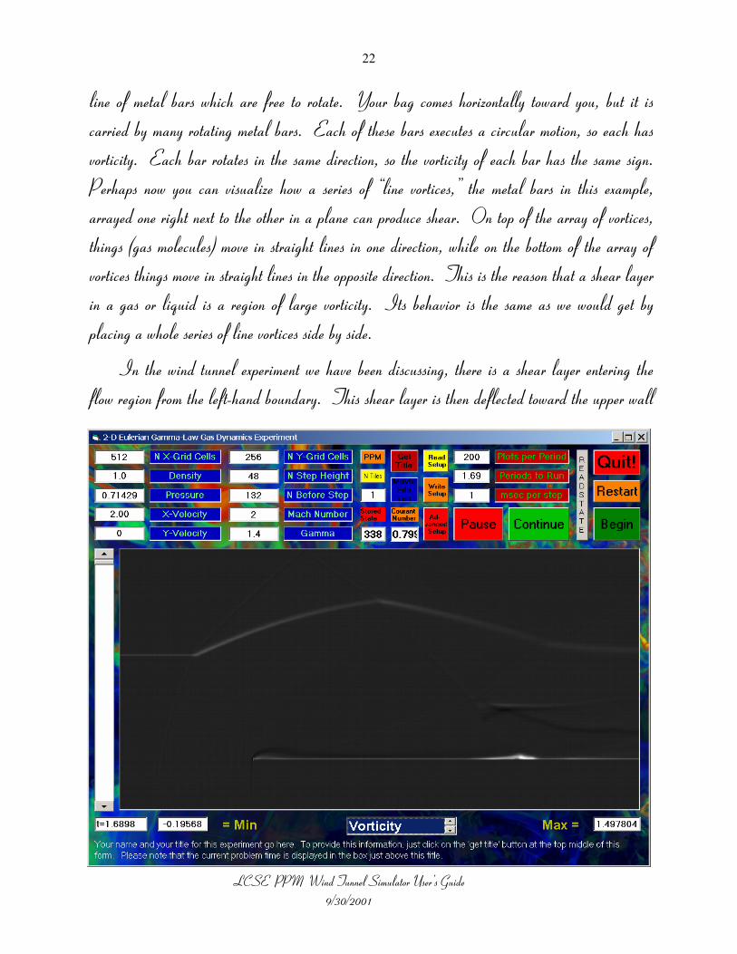
In the wind tunnel experiment we have been discussing, there is a shear layer entering the flow region from the left-hand boundary. This shear layer is then deflected toward the upper wall


23

by the bow shock, and it is deflected once more back away from the upper wall by the reflection of the bow shock. The shear layer is a region of strong vorticity. Thus it should stand out if we were to make a plot of the vorticity in our wind tunnel flow. Such a plot is shown on the previous page. As expected, the shear layer stands out. However, you will note that the strongest vorticity is located in a shear layer right along the top of the step in the wind tunnel. This is not surprising. Even if the friction of the step’s upper surface is assumed to be negligible, as it is in the wind tunnel simulator program, this air would have to have come from the region of nearly stagnant air right in front of the step. It would have turned sharply around the corner of the step, and it is not surprising that it ends up traveling more slowly downstream than the air just a little bit above it, whose progress was far less obstructed by the presence of the step. A couple of other shear layers show up in the vorticity picture. These are formed from the intersection of 3 shock fronts by a mechanism that is too complex to discuss here.

The wind tunnel simulator provides us with multiple ways to visualize the velocity field of this rather complex flow. You can make up your own mind about it, but to me it is not so useful to make plots of the separate x and y velocity components. The reason for this in general is that there is nothing special about either the x or the y directions. Actually, in our wind tunnel, these directions are indeed special ones. Nevertheless, features in the flow, like the various shock fronts and shear layers, do not align themselves with these two special directions. We might well wish to know the change across a shear layer of the velocity in the direction along its length, but we can only get this from examining the x and y velocity components by going through some algebra, with sine and cosine functions thrown in. So, often in practice, and particularly for 3-D flows, we choose to visualize a velocity field in some way other than making pictures of the individual distributions of its x and y components.

The smoke streams that we inject into our wind tunnel flow represent one very effective way to visualize a velocity field. The smoke particles are tracers that are passively carried along with the flow, showing us where and how fast it is going in the process. The eye is not so good at following


24

individual tracer particles, so we have injected continuous streams of smoke instead. In 3-D, following lots of individual particles becomes especially difficult, because depth perception is hard to achieve. But streams of smoke work very well. In this example of the wind tunnel we have already encountered a drawback of using streams of smoke. They cannot reveal to us shear in the flow field unless the shear layers cross the streams of smoke. This problem can be addressed by injecting smoke into the wind tunnel in a checkerboard pattern. If each square of the checkerboard is several cells on a side when it is injected, we should be able to follow the distortions introduced by the flow field without having the pattern all blend together. Shear in any direction is easily detected in such a pattern.

Another way to view the velocity field is to make a movie of the changing distribution of some variable, like the entropy, that tends to be simply carried along with the flow. This technique serves two goals simultaneously – it visualizes both the entropy distribution and the velocity field. Such a display takes some care to interpret, but it is very powerful. Actually, the vorticity distribution, which is derived directly from the velocity field, tends to be carried along with the flow. Therefore making movies of the vorticity distribution can be a powerful means for under-standing the velocity field. One must build up a skill for interpreting such visualizations, but one is rewarded for doing so by their ability to communicate so much information at one viewing.

We have already mentioned the vorticity. It represents the intensity of swirling (or shear) flow. It is therefore derived from the velocity field, and it tells us something very specific about it. The vorticity is one of a number of quantities that we can visualize that show us where something changes and that ignore regions in which that something has no change. The velocity in our wind tunnel flow changes suddenly across the shear layer, and the shear layer is highlighted in the vorticity plot. Along the top of the step, the velocity also changes sharply, and this shear layer is also highlighted in the vorticity plot. However, not all velocity changes are highlighted by the vorticity. At the shock fronts in the flow the velocity changes suddenly, but there is very little vorticity associated with these sudden velocity changes. That is because shock fronts compress the


25

gas in the direction perpendicular to the front. This simple, one-dimensional compression generally does not produce much shear, and hence little vorticity. To highlight the changes in the velocity at the shock fronts, we need to look at the distribution of something called the divergence of the velocity field.

The divergence of the velocity field, as its name implies, measures the extent to which the velocity field corresponds to a diverging flow that causes the gas to expand and the gas density to decrease. The velocity divergence can be positive or negative. Negative values correspond to converging flow and compression of the gas. One of the selections you can make for a visualization of your wind tunnel experiment is the negative divergence of the velocity. In such a display, shown below, the shock fronts are highlighted, since they correspond to regions of strong compression. The strongly diverging flow right near the corner of the step also shows up prominently in this plot. It


26

is interesting to compare this plot of the negative velocity divergence with the plot of the vorticity. Notice that each display brings out a different and complementary set of flow features.

There is another display of this type that we can make which will bring out both these sets of flow features at once. It is therefore a more difficult display to interpret, because it is not immediately clear from the display which kind of sudden change is being shown. This new sort of display is called a shadowgraph. It is a classical flow visualization technique, and you can find many examples of it in the Album of Fluid Motion. In the laboratory, shadowgraphs are made by taking photographs of fluid flows. The photos show sudden changes in gas density and make regions in which the density changes slowly and smoothly invisible. This effect results from the dependence on density of the index of refraction of the gas, which causes sharp changes in gas density to be traced by side-by-side pairs of bright and dark lines. This kind of photo shows a


27

quantity known as the Laplacian of the density. The Laplacian is large in magnitude wherever the density is very different from the average of the densities at all points along a circle of small radius centered on that point. Thus a sharp density spike will stand out in a shadowgraph, but also the Laplacian of the density will be large all along a front at which the density changes suddenly. In our wind tunnel flow we therefore expect to see all the shocks, all the shear layers (because they all have sharp density changes across them in this flow), and the nearly evacuated spot right near the corner of the step to stand out prominently in a shadowgraph display. Such a display, which you can select using the wind tunnel simulator, is shown on the previous page.

In the above discussion, we have seen how we can use the wide variety of flow visualizations available with the wind tunnel simulator to analyze what is happening in a developing flow. In this document, we have included snap shots at one time only in order to illustrate this process. But of course the simulator program can produce animations of all these types of displays. With enough room on our screen, we could animate all these types of visualizations simultaneously to give a complete picture of the flow. Another technique would be to exploit the symmetry of this sort of flow to make a composite view of several different variables at once, as in the image on the next page, which shows the density in the top half and the smoke streams in the bottom. This image was pieced together using Photoshop, but it is easy to revise the wind tunnel simulator to produce images of this type and to animate them upon demand.


28


29

Appendix: Time Development of the Wind Tunnel Flow On the following pages, as a sort of appendix, the time development of the density distribution

is shown from the run that was discussed above. Several snap shots capture the flow at interesting stages, which are annotated below the images.


30

Here we see the flow during its initial development. The gas entering at the left piles up against the step, forming the bow shock. This shock is moving rapidly forward, because the amount of gas escaping by flowing up and around the step is not enough to balance the gas that continues to slam into the step, striking the bow shock. The gas density and pressure at the left-hand boundary was not originally in balance with the new gas just entering through that boundary. This has caused the gas originally in the wind tunnel to expand into the incoming gas, driving a weak shock into this incoming stream. The jump in the gas density which marks the boundary between the denser gas originally in the wind tunnel and the less dense gas entering it since the run began is easily seen, even as it passes through the bow shock and into the region of highly compressed gas right in front of the step.

Rarefaction wave working its way into the gas originally in the wind tunnel.

Boundary between gas originally in the wind tunnel and newly entering gas.

Weak shock moving into & decelerating inflowing gas.

Bow shock.


31

Here we see that the bow shock has moved up the channel and that it is interacting with the boundary between the air originally in the wind tunnel and the air that is now entering it. A shock also forms where air rushing around the corner of the step strikes the top surface of the step and is compressed and its velocity redirected straight down the wind tunnel. A vortex is beginning to form right where the shear layer crosses the boundary between the original gas in the wind tunnel and the gas that has entered since the run began.

Shear layer with faster flow and denser air above than below.

Shock compressing air flowing around corner & striking step top


32

Bow shock travels more slowly into denser gas above the shear layer.

Weak reflected shock waves formed when the bow shock struck the denser air above the shear layer.

Shock travels more slowly in denser air above shear layer, so it forms this complicated bend to meet faster shock below.


33

Bow shock reflects from shear layer.

Bow shock works its way up toward upper wall.


34

Here we see the bow shock just beginning to reflect off of the upper wall of the wind tunnel.


35

Here the reflected shock wave from the upper wall is beginning to work its way back down across the channel. The structures within the flow caused by the density and pressure mismatches between the air originally inside the wind tunnel and that which has been entering since the run began are finally beginning to be swept downstream and out of this section of the wind tunnel. You can follow their progress on and out over the next few images in this sequence.


36


37


38

This is about the last image in which you can trace the shock that is reflected from the bow shock where it strikes the shear layer. That very weak shock strikes the top of the step at the location of a small region of lower density in which the flow recirculates (that is, it moves upstream along the surface of the step within this little “recirculation bubble”).


39

The reflection of the bow shock at the shear layer is now essentially invisible. A weak shock can be seen extending nearly vertically into the flow above the little recirculation bubble where this reflected shock once struck the upper surface of the step.


40

Here we see the reflection of the bow shock from the upper wall is just beginning to reflect again from the top of the step. If we could see more of the length of this wind tunnel, eventually we would see this shock bounce back and forth across the channel, getting weaker with each reverberation. Note how the shear layer kinks each time it passes through another shock wave.


41

Here we see that the reflected bow shock is beginning to strike the little recirculation bubble located on the top surface of the step.


42

Here we see, at the time when we stopped the simulation, that the reflected bow shock has passed through the little recirculation bubble, creating a complex and interesting, but transient structure.


43

Appendix 2: How to Play Back a Movie of Your Experiment After you exit from the wind tunnel experiment program by clicking on the big, red “Quit!”

button at the upper right corner of the form, the images that were displayed in the form’s picture box when you navigated with the vertical scroll bar at the left-hand edge of the form remain stored on your hard disk. These images are each Microsoft Windows bitmap files, a standard display format that you can view in most image editing programs, or which you can import into WORD or PowerPoint documents. However, you might wish to be able to animate them as you did while your experiment was running. This can be done by starting up the “PPM2Dgui.exe” or the “PPM2DguiSmallForm.exe” application once more on your computer. When, as described on page 5 of this manual, you are prompted to provide through the use of the file system browser window a stem name for files that this program will write on your disk, use this browser window to navigate to the directory on your disk where you wrote your sequence of bitmap files from your earlier run. Then click on the “Open” button or press the “Enter” key. Now the program will wait for you to specify the parameters of your run and then to click on the “Begin” button. Do not do that. Instead, at this point you should click on the blue button labeled “Movie File List” that is located near the upper center portion of the form. This will cause another file system browser window to pop up. In this window, navigate to the directory in which you wrote the bitmap files you want to review and locate and double click on the file in that directory that contains the list of these files. That file should end in “MovieFileList.txt” and thus be easy to recognize. Double clicking on this file in the browser window will cause it to be read in, and your form will change the values of its settings. In particular, the vertical scroll bar at the left-hand edge of the form will be redrawn to reflect the entire series of your stored bitmap images. Now you can animate these images with the program just as you were able to do when you originally ran the program and created these images with it. The correct values of the times associated with these snap shot images and of the minimum and maximum values of the variable displayed will be placed in the appropriate text-box labels on the form.


44

Acknowledgements: The Wind Tunnel Simulator utility described above is used in the development and testing

of new numerical methods for computational fluid dynamics. That development in the LCSE has been supported by the Department of Energy through the Office of Science and through the ASCI program. It has also been supported in part, especially in its application to large parallel computing systems, by the NSF through its PACI program. Support to the LCSE through the University of Minnesota’s Minnesota Supercomputing Institute is also gratefully acknowledged.

Paul Woodward Sept. 30, 2001...Running the 2-D Wind Tunnel Program Paul Woodward Sept. 30, 2001 The...

Documents

Transcript of Paul Woodward Sept. 30, 2001...Running the 2-D Wind Tunnel Program Paul Woodward Sept. 30, 2001 The...