Patterns of language variation and underlying linguistic...
14
Patterns of language variation and underlying linguistic features: a new dialectometric approach SIMONETTA MONTEMAGNI / MARTIJN WIELING / BOB DE JONGE / JOHN NERBONNE 1. INTRODUCTION For almost forty years quantitative methods have been applied to the analysis of dialect variation: these methods focused mostly on identifying the most important dialectal groups using an aggregate analysis of the linguistic data (Séguy 1973; Goebl 1984; Nerbonne et al. 1999). While viewing dialect differences at an aggregate level certainly gives a more comprehensive view than the analysis of subjectively selected features, the aggregate approach has never fully convinced linguists of its use as it fails to identify the linguistic distinctions among the identified groups. Michele Loporcaro (2009) criticizes that dialectometry measures the structural distances among dialectal varieties without passing through a rationalization of the linguistic structure. Recently, Wieling and Nerbonne (2010, 2011) proposed a promising graph-theoretic method, the spectral partitioning of bipartite graphs, to cluster varieties and simultaneously determine the underlying linguistic basis. Their results for Dutch are promising, and this method can be taken as an answer to Loporcaro‟s criticism, since it permits one to reconstruct which features underlie the aggregate patterns of dialectal variation and the role played by each of them. In this way, the gap between models of linguistic variation based on quantitative analyses and more traditional analyses based on specific linguistic features is significantly reduced. This paper illustrates the application of this technique on the dialectal corpus of the Atlante Lessicale Toscano (ALT) 1 and discusses the results. The atlas material contains phonetic transcriptions even though the published atlas documents lexical variation. Our analysis focuses on the level of phonetic variation. As documented 1 ALT (Giacomelli et al. 2000) is available as an on-line resource, ALT-Web, http://serverdbt.ilc.cnr.it/ALTWEB/.
-
Upload
duongduong -
Category
Documents
-
view
216 -
download
0
Transcript of Patterns of language variation and underlying linguistic...
Patterns of language variation and underlying linguistic
features: a new dialectometric approach
SIMONETTA MONTEMAGNI / MARTIJN WIELING / BOB DE JONGE / JOHN NERBONNE
1. INTRODUCTION
For almost forty years quantitative methods have been applied to the analysis of dialect variation:
these methods focused mostly on identifying the most important dialectal groups using an aggregate
analysis of the linguistic data (Séguy 1973; Goebl 1984; Nerbonne et al. 1999). While viewing
dialect differences at an aggregate level certainly gives a more comprehensive view than the
analysis of subjectively selected features, the aggregate approach has never fully convinced
linguists of its use as it fails to identify the linguistic distinctions among the identified groups.
Michele Loporcaro (2009) criticizes that dialectometry measures the structural distances among
dialectal varieties without passing through a rationalization of the linguistic structure.
Recently, Wieling and Nerbonne (2010, 2011) proposed a promising graph-theoretic method,
the spectral partitioning of bipartite graphs, to cluster varieties and simultaneously determine the
underlying linguistic basis. Their results for Dutch are promising, and this method can be taken as
an answer to Loporcaro‟s criticism, since it permits one to reconstruct which features underlie the
aggregate patterns of dialectal variation and the role played by each of them. In this way, the gap
between models of linguistic variation based on quantitative analyses and more traditional analyses
based on specific linguistic features is significantly reduced. This paper illustrates the application of
this technique on the dialectal corpus of the Atlante Lessicale Toscano (ALT)1 and discusses the
results. The atlas material contains phonetic transcriptions even though the published atlas
documents lexical variation. Our analysis focuses on the level of phonetic variation. As documented
1 ALT (Giacomelli et al. 2000) is available as an on-line resource, ALT-Web, http://serverdbt.ilc.cnr.it/ALTWEB/.
in Montemagni (2008), this is the level for which an aggregate analysis of the ALT dialectal corpus
differs from the analyses by Giannelli (2000) and Pellegrini (1977). Phonetic variation in Tuscany
thus provides a challenging case study to test this new technique.
Two additional contributions of this paper are technical: first, we weight sound
correspondences by their frequency in order to emphasize more common correspondences, and
second, we introduce a means of tracking correspondences in their phonetic context. As sound
changes are recognized to be conditioned by phonetic context, this modification should result in
detection that is not only more sensitive, but also linguistically better founded.
2. THE DATA SOURCE
2.1. The Atlante Lessicale Toscano
The ALT is a regional linguistic atlas focusing on dialectal variation throughout Tuscany, a region
where both Tuscan and non-Tuscan2 dialects are spoken. ALT interviews were carried out in 224
localities of Tuscany, with 2193 informants selected with respect to socio-demographic parameters,
on the basis of a questionnaire of 745 items designed to elicit mainly lexico-semantic variation.
In ALT, each dialectal item is assigned a multi-level representation: for this study, we focused
on the phonetic transcription and normalized representation levels where the latter is meant to
abstract away from phonetic variation within Tuscany. At this level, neutralization is only
concerned with phonetic variants resulting from productive phonetic processes (e.g. variants
involving spirantization or voicing of plosives like //, as in [skjaa] and [skjada]), while it
does not deal with morphological variation nor unproductive phonetic processes. The alignment of
the different representation levels was exploited to automatically extract all attested phonetic
variants (PV) sharing the same normalized form (NF). Due to the features of the normalized
2 This is the case for dialects in the north, namely Lunigiana and small areas of the Apennines, which belong to the
group of Gallo-Italian dialects.
representation level, we can be sure that patterns of variation emerging from the analysis of PVs of
the same NF document only genuine phonetic processes.
2.2. Building the experimental dataset
In this study, ALT dialectal data were used in a quite peculiar way, namely as a corpus: i.e. we did
not start from a predefined set of questionnaire items specifically designed to investigate the
geographic distribution of phonetic features, but rather from the set of the attested ALT lexical
items, which were elicited from informants for quite different (mainly, lexico-semantic) purposes.
By using atlas data as a corpus, the problem of inherently subjective feature selection is
significantly reduced, thus providing a more “realistic” linguistic signal (Szmrecsanyi, to appear).
On the other hand, by using atlas data as a corpus one of the main advantages usually ascribed to
atlas-based studies, namely the areal coverage of dialectal items, can no longer be taken for granted.
To overcome this potential problem, we enforced a minimal areal coverage threshold when
selecting NFs (see below).
In particular, we focused on the phonetic variants of NFs selected from the ALT dialectal
corpus based on both linguistic and geographical criteria. With respect to syntax only nouns and
adjectives were selected,3 both as single words and multi-word expressions.4 Phonetic variability
represented the other linguistic criterion: NFs were selected where the number of PVs ranged from
5 to 34 (the maximum number of PVs attested for one NF). Geographical criteria included: i) the
areal coverage of selected NFs, which we required to be ≥ 100 (out of 224) locations; ii) the
locations investigated which included 213 (out of the 224) locations where Tuscan dialects are
spoken. The resulting dataset included 444 NFs (4.64% of all diatopically varying NFs), for a total
of 502,799 phonetically variant tokens.
3 As in ALT verbal answers are represented by different inflected forms not always explicitly marked, verbs were
excluded from the experimental dataset to prevent potential noise deriving from verbal morphology.
4 Note that selected multi-word expressions were represented by “frozen” word combinations.
In order to test the representativeness of the selected sample of 444 NFs with respect to the
whole set of NFs having at least two PVs attested in at least two locations (used in Montemagni
2008), we measured the correlation between overall phonetic distances and phonetic distances
focusing on the selected sample which turned out to be very high (r = 0.994). We can thus conclude
that the selected sample can be usefully exploited to reliably study the patterns of phonetic variation
in Tuscany.
Since in the proposed analysis method PVs recorded in each location are compared with those
attested in a reference variety, the experimental dataset also included the phonetic realization of the
selected NFs in standard Italian.
3. METHODS
3.1. Extracting sound correspondences
Every variety attested in a given location is described in terms of the realizations of a given
phonetic segment with respect to a reference variety (i.e. standard Italian). Attested phonetic
realizations are encoded in terms of sound correspondences (SCs) linking the dialectal allophone
with its realization in the reference variety.
SCs are obtained by aligning the PVs of a NF in a variety with its reference realization
(standard Italian) on the basis of an adapted Levenshtein algorithm (Levenshtein 1965). The regular
Levenshtein algorithm aligns two strings by minimizing the number of insertions, deletions and
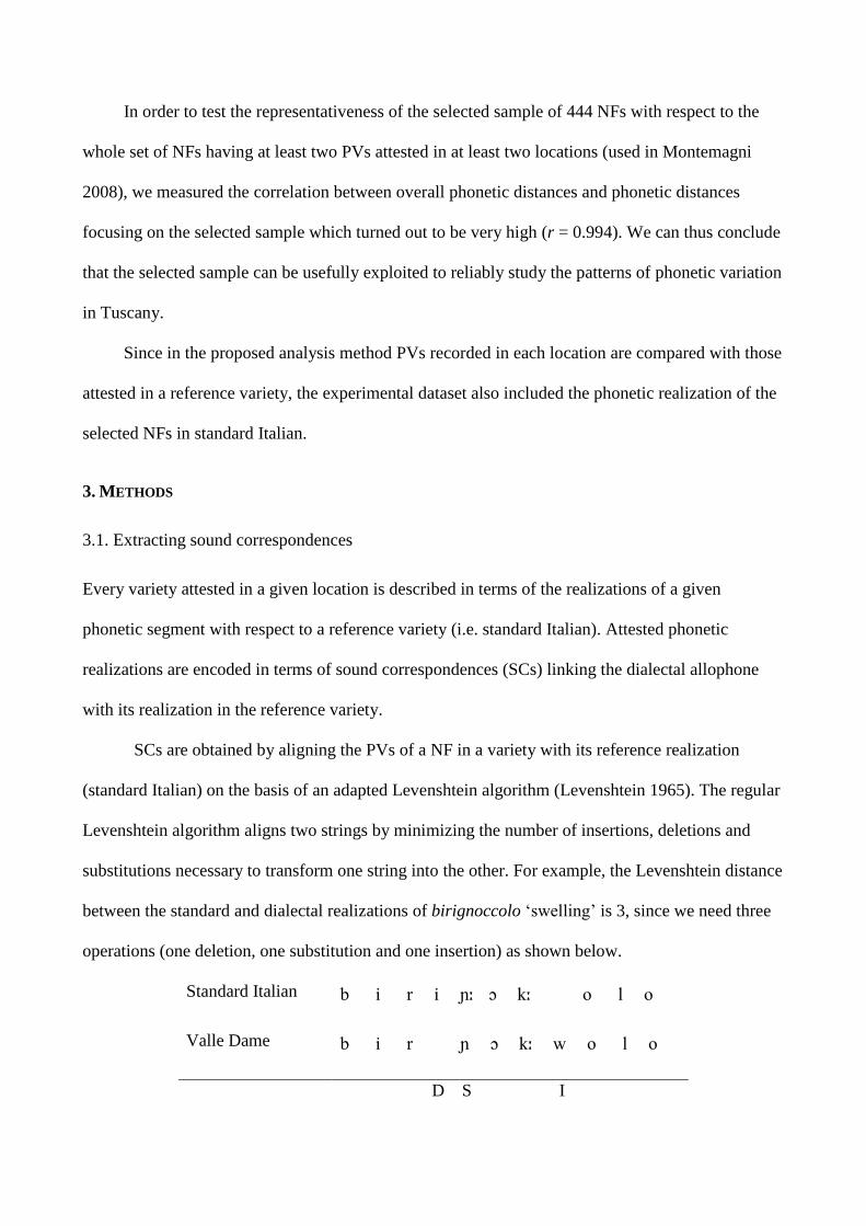
substitutions necessary to transform one string into the other. For example, the Levenshtein distance
between the standard and dialectal realizations of birignoccolo „swelling‟ is 3, since we need three
operations (one deletion, one substitution and one insertion) as shown below.
Standard Italian
Valle Dame
D S I
Instead of the simple Levenshtein algorithm, we used a more sensitive version which uses
automatically determined phonetic distances to increase the quality of the alignments (for more
details see Wieling et al. 2009; Wieling and Nerbonne, accepted).
Since for each location investigated there was a socio-demographically differentiated group
of informants potentially giving rise to multiple responses, we represented the variety with the most
frequent phonetic variant of each selected normalized form.
The PV alignments exemplified above are used to identify SCs. We focus on phonetic
correspondences involving non-identical segments and insertions and deletions, as these are most
interesting. We also ignore SCs occurring infrequently (in fewer than 25 varieties) in a single word
only.5 Due to the fact that in the ALT dataset the same SC could originate from different phonetic
processes, we decided to enrich their representation with contextual information, i.e. for each SC we
also identify the left and right (single segment) context. As context, we only distinguish consonants,
vowels, semi-vowels, a gap (in the case of an insertion or a deletion) and the word boundary (for the
initial and final segment of a word). For instance, the SC []#[] in the example above is recorded
as V[]V#G[]V indicating that there are vowels to the left and right of [] and that there is a
vowel to the right and a gap to the left of [].
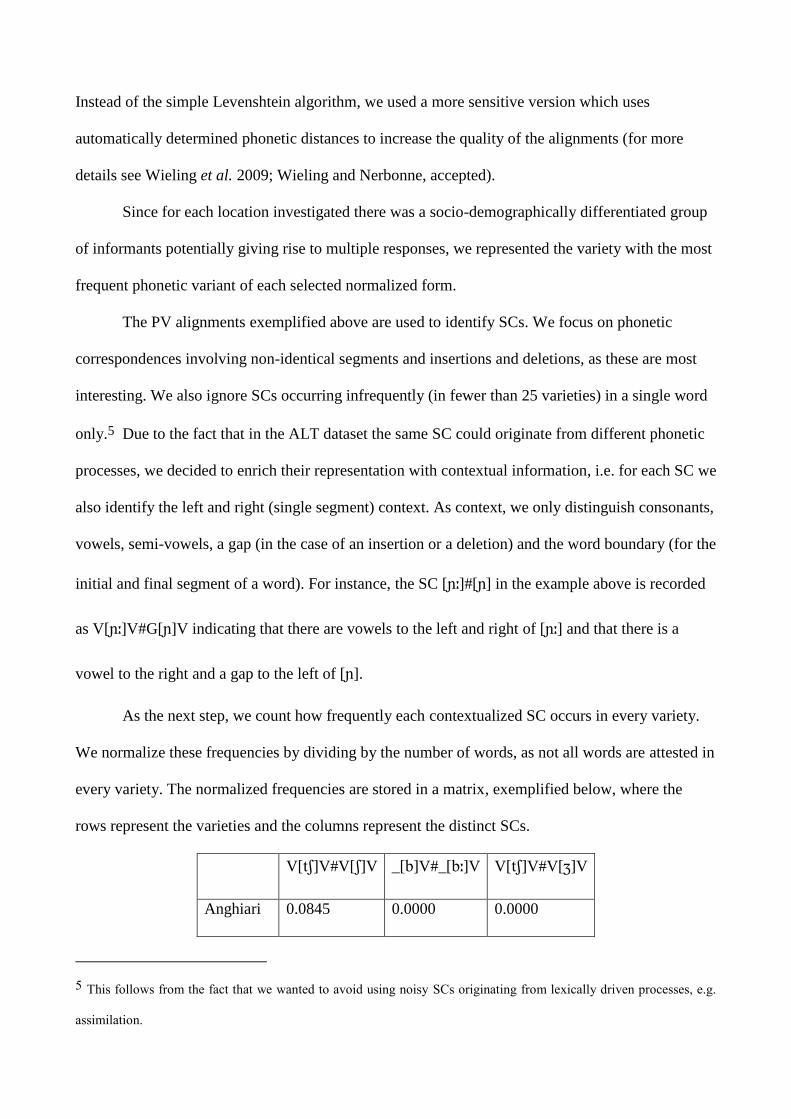
As the next step, we count how frequently each contextualized SC occurs in every variety.
We normalize these frequencies by dividing by the number of words, as not all words are attested in
every variety. The normalized frequencies are stored in a matrix, exemplified below, where the
rows represent the varieties and the columns represent the distinct SCs.
V[]V#V[]V _[]V#_[]V V[]V#V[]V
Anghiari 0.0845 0.0000 0.0000
5 This follows from the fact that we wanted to avoid using noisy SCs originating from lexically driven processes, e.g.
assimilation.
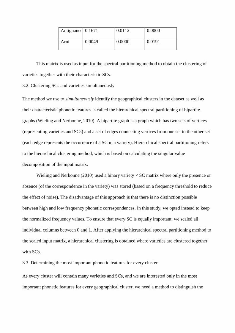
Antignano 0.1671 0.0112 0.0000
Arni 0.0049 0.0000 0.0191
This matrix is used as input for the spectral partitioning method to obtain the clustering of
varieties together with their characteristic SCs.
3.2. Clustering SCs and varieties simultaneously
The method we use to simultaneously identify the geographical clusters in the dataset as well as
their characteristic phonetic features is called the hierarchical spectral partitioning of bipartite
graphs (Wieling and Nerbonne, 2010). A bipartite graph is a graph which has two sets of vertices
(representing varieties and SCs) and a set of edges connecting vertices from one set to the other set
(each edge represents the occurrence of a SC in a variety). Hierarchical spectral partitioning refers
to the hierarchical clustering method, which is based on calculating the singular value
decomposition of the input matrix.
Wieling and Nerbonne (2010) used a binary variety × SC matrix where only the presence or
absence (of the correspondence in the variety) was stored (based on a frequency threshold to reduce
the effect of noise). The disadvantage of this approach is that there is no distinction possible
between high and low frequency phonetic correspondences. In this study, we opted instead to keep
the normalized frequency values. To ensure that every SC is equally important, we scaled all
individual columns between 0 and 1. After applying the hierarchical spectral partitioning method to
the scaled input matrix, a hierarchical clustering is obtained where varieties are clustered together
with SCs.
3.3. Determining the most important phonetic features for every cluster
As every cluster will contain many varieties and SCs, and we are interested only in the most
important phonetic features for every geographical cluster, we need a method to distinguish the
most important SCs. Following Wieling and Nerbonne (2011), we define the importance of a SC in
a cluster as a linear combination of two measures, distinctiveness and representativeness.
The representativeness of a SC measures how frequently the SC occurs within the cluster.
E.g., if there are ten varieties in the cluster and the sum of the normalized frequencies equals 4, the
representativeness equals 0.4 (4/10).
The distinctiveness of a SC measures how frequently the SC occurs within a cluster as
opposed to outside of the cluster, taking the relative size of the cluster into account. E.g., if the SC
does not occur outside of the cluster, the distinctiveness is 1 (the phonetic correspondence perfectly
distinguishes the cluster from the rest), no matter how large the cluster. Alternatively, if a cluster
contains 50% of the varieties and 50% (or less) of the total sum of the normalized frequencies, the
distinctiveness is 0 (the phonetic correspondence does not distinguish the cluster at all).
The values of distinctiveness and representativeness range between 0 and 1. Normally
representativeness and distinctiveness are averaged to obtain the importance score for every SC
(higher is better). In this study we decided to weight representativeness twice as heavily as
distinctiveness since our matrix contained many infrequent (non-informative) SCs, whose
distinctiveness was very high.
4. RESULTS
The results obtained are based on 208 SCs extracted from the analysis of the PVs of 444 NFs. By
classifying the SCs extracted according to the type of phonetic segments involved, it turns out that
Tuscan phonetic variation is mainly concerned with consonants: i.e. 70% are consonantal SCs
against 25% which are vocalic and 5% which involve semi-vowels.
4.1. Geographical results
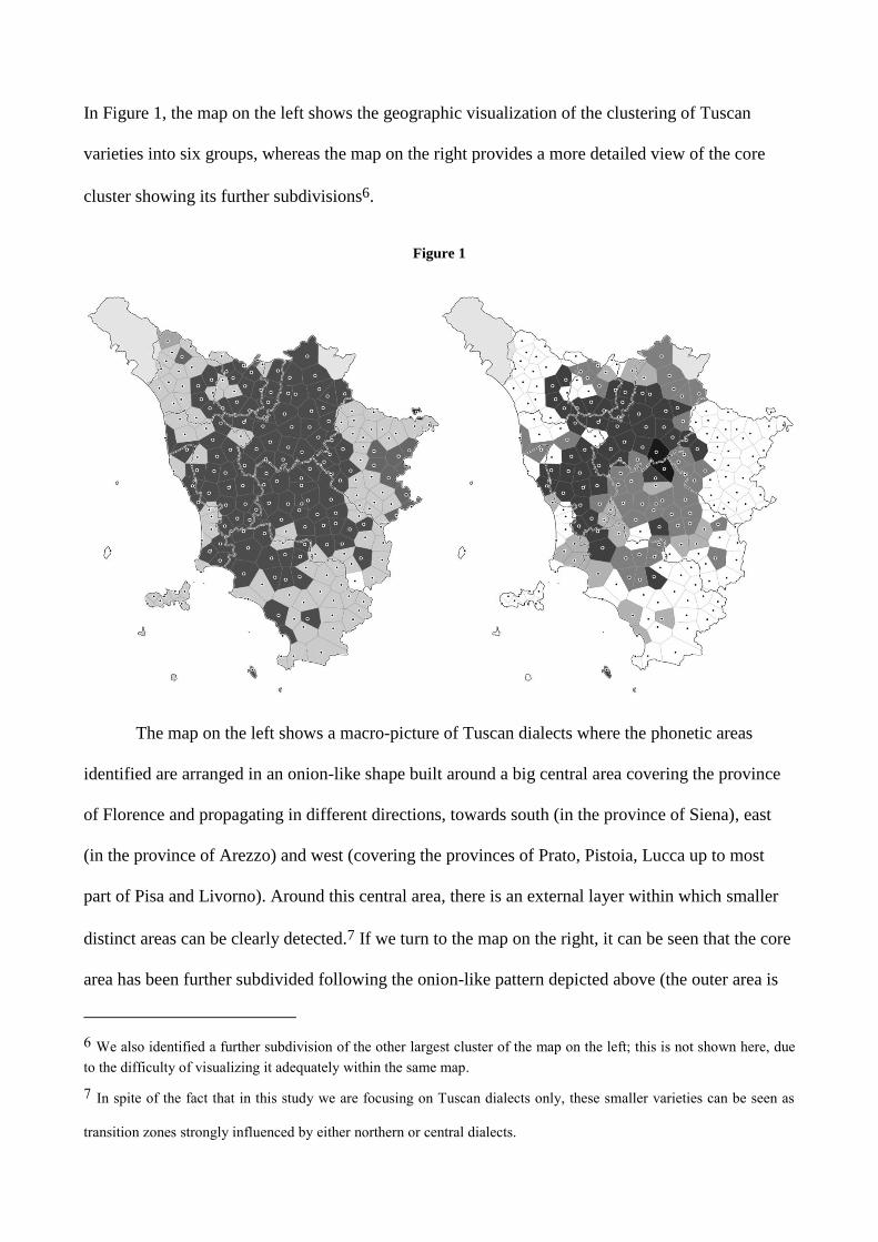
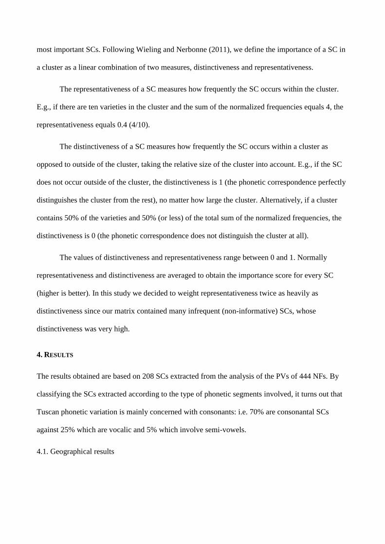
In Figure 1, the map on the left shows the geographic visualization of the clustering of Tuscan
varieties into six groups, whereas the map on the right provides a more detailed view of the core
cluster showing its further subdivisions6.
Figure 1
The map on the left shows a macro-picture of Tuscan dialects where the phonetic areas
identified are arranged in an onion-like shape built around a big central area covering the province
of Florence and propagating in different directions, towards south (in the province of Siena), east
(in the province of Arezzo) and west (covering the provinces of Prato, Pistoia, Lucca up to most
part of Pisa and Livorno). Around this central area, there is an external layer within which smaller
distinct areas can be clearly detected.7 If we turn to the map on the right, it can be seen that the core
area has been further subdivided following the onion-like pattern depicted above (the outer area is
6 We also identified a further subdivision of the other largest cluster of the map on the left; this is not shown here, due
to the difficulty of visualizing it adequately within the same map.
7 In spite of the fact that in this study we are focusing on Tuscan dialects only, these smaller varieties can be seen as
transition zones strongly influenced by either northern or central dialects.
ignored, and colored white), i.e. a new intermediate layer has appeared between the external layer
and the core: a new core covers a more restricted area revolving around Florence and expanding in
all directions, in particular west and south.
The phonetic areas identified follow the pattern reported in Montemagni (2007, 2008), but
they differ from the analyses by Pellegrini (1977) and Giannelli (2000), where the former is based
on the distribution of phonetic phenomena and the latter results from the simultaneous consideration
of phonetic, phonemic, morpho-syntactic and lexical features. In both cases, it is interesting to note
that the proposed dialects from a) the Florentine area, b) the Siena area and c) the western areas
(Pisano-Livornese) cannot be clearly identified in Figure 1.
4.2. Linguistic results
For what concerns the underlying linguistic features, let us first focus on the dialectal clusters in the
left map. The SCs underlying the core area in the left map cover different phonetic phenomena:
more than half of the segment pairs correspond to spirantization phenomena involving both
voiceless and voiced stops // as well as // in different contexts and with different
outcomes, e.g.: the SC []#[] occurring in the contexts V[_]V#V[_]V, V[_]C#V[_]C and
_[_]V#_[_]V as in [] vs [], [] vs [], [] vs []
respectively; or the SCs V[]V#V[]V, V[]V#V[]V and V[]V#V[-]V as in [] vs
[] or [] or []. Other highly ranked features are represented by the
rhoticism of preconsonantal // (as in [] vs []) and phonotactic lengthening in
word initial position (as in [] vs []). In the external layer, the list of underlying
phonetic features is much longer and more heterogeneous. Among the top features we note SCs
corresponding to: spirantization phenomena involving the voiceless velar stop // (characterized by
a stronger but still spirant realization, as in [] vs []) and the affricates // and
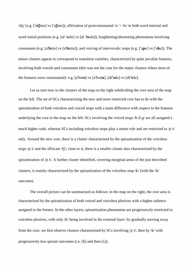
// (e.g. [] vs []); affrication of postconsonantal // > // in both word internal and
word initial positions (e.g. [] vs []); lengthening/shortening phenomena involving
consonants (e.g. [] vs []); and voicing of intervocalic stops (e.g. [] vs []). The
minor clusters appear to correspond to transition varieties, characterized by quite peculiar features,
involving both vowels and consonants (this was not the case for the major clusters where most of
the features were consonantal): e.g. [] vs [], [] vs [].
Let us turn now to the clusters of the map on the right subdividing the core area of the map
on the left. The set of SCs characterizing the new and more restricted core has to do with the
spirantization of both voiceless and voiced stops with a main difference with respect to the features
underlying the core in the map on the left: SCs involving the voiced stops // are all assigned a
much higher rank, whereas SCs including voiceless stops play a minor role and are restricted to //
only. Around the new core, there is a cluster characterized by the spirantization of the voiceless
stops // and the affricate //; close to it, there is a smaller cluster also characterized by the
spirantization of //. A further cluster identified, covering marginal areas of the just described
clusters, is mainly characterized by the spirantization of the voiceless stop // (with the //
outcome).
The overall picture can be summarized as follows: in the map on the right, the core area is
characterized by the spirantization of both voiced and voiceless plosives with a higher salience
assigned to the former. In the other layers, spirantization phenomena are progressively restricted to
voiceless plosives, with only // being involved in the external layer: by gradually moving away
from the core, we first observe clusters characterised by SCs involving //, then by // with
progressively less spirant outcomes (i.e. [] and then []).
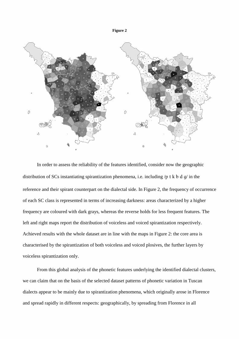
Figure 2
In order to assess the reliability of the features identified, consider now the geographic
distribution of SCs instantiating spirantization phenomena, i.e. including / / in the
reference and their spirant counterpart on the dialectal side. In Figure 2, the frequency of occurrence
of each SC class is represented in terms of increasing darkness: areas characterized by a higher
frequency are coloured with dark grays, whereas the reverse holds for less frequent features. The
left and right maps report the distribution of voiceless and voiced spirantization respectively.
Achieved results with the whole dataset are in line with the maps in Figure 2: the core area is
characterised by the spirantization of both voiceless and voiced plosives, the further layers by
voiceless spirantization only.
From this global analysis of the phonetic features underlying the identified dialectal clusters,
we can claim that on the basis of the selected dataset patterns of phonetic variation in Tuscan
dialects appear to be mainly due to spirantization phenomena, which originally arose in Florence
and spread rapidly in different respects: geographically, by spreading from Florence in all
directions, especially southward and westward; and phonologically, by originally involving the
velar stop //, then // up to the voiced stops //.
5. CONCLUSION
In this paper we illustrated the application of the hierarchical spectral partitioning of bipartite
graphs technique on the ALT dialectal corpus and discussed the results. The contribution of this
study is twofold. From the point of view of Tuscan dialectology, it helps gain insight into the nature
of phonetic variation in Tuscany, by simultaneously providing a classification of dialectal varieties
and their underlying linguistic basis. Obviously, these results need further investigation in different
directions. First, it would be interesting to enlarge the dataset to check whether identified variation
patterns and underlying features change and to what extent; achieved results for what concerns
spirantization phenomena should be analyzed in the light of the primary texts on the topic of Gorgia
Toscana (Giannelli and Savoia, 1978, 1980). Second, due to the simultaneous diatopic and diastratic
characterisation of the ALT data, it would be interesting to extend this study by considering socio-
economical factors playing a role in the phonetic variation process as well. Experiments are
currently being carried out by using Latin as a reference language, instead of standard Italian. On
the technical side, this study gave us the opportunity to design a contextualised representation of
SCs resulting in a better founded analysis of underlying phonetic features and to explore the role of
frequency of phonetic features in the study of dialectal variation.
Acknowledgements
The research reported in this paper was carried out in the framework of the Short Term Mobility
program of international exchanges funded by CNR (Italy).
Bibliography
LEVENSHTEIN 1965 = VLADIMIR LEVENSHTEIN, Binary codes capable of correcting deletions,
insertions and reversals, in «Doklady Akademii Nauk SSSR», 163, 1965, pp. 845-848.
GIACOMELLI et al. 2000 = GABRIELLA GIACOMELLI ‒ LUCIANO AGOSTINIANI ‒ PATRIZIA BELLUCCI ‒
LUCIANO GIANNELLI ‒ SIMONETTA MONTEMAGNI ‒ ANNALISA NESI ‒ MATILDE PAOLI ‒
EUGENIO PICCHI ‒ TERESA POGGI SALANI (eds.), Atlante Lessicale Toscano, Lexis Progetti
Editoriali, Roma, 2000.
GIANNELLI 2000 = LUCIANO GIANNELLI, Toscana, Pacini Editore, Pisa, 2000 (1976, first edition).
GIANNELLI ‒ SAVOIA 1978 = LUCIANO GIANNELLI ‒ LEONARDO M. SAVOIA, L’indebolimento
consonantico in Toscana (I.), in «Rivista Italiana di Dialettologia», Vol. 2, 1978, pp. 23-58.
GIANNELLI ‒ SAVOIA 1980 = LUCIANO GIANNELLI ‒ LEONARDO M. SAVOIA, L’indebolimento
consonantico in Toscana (II.), in «Rivista Italiana di Dialettologia», Vol. 4, 1979-80, pp. 38-
101.
GOEBL 1984 = HANS GOEBL, Dialektometrische Studien: Anhand italoromanischer,
rätoromanischer und galloromanischer Sprachmaterialien aus AIS und ALF, Tübingen,
Niemeyer, 1984.
LOPORCARO 2009 = MICHELE LOPORCARO, Profilo linguistico dei dialetti italiani, Roma-Bari,
Laterza 2009.
MONTEMAGNI 2007 = SIMONETTA MONTEMAGNI, Patterns of phonetic variation in Tuscany: using
dialectometric techniques on multi-level representations of dialectal data, in Proceedings of
the Workshop on Computational Phonology at RANLP-2007, 26 September 2007, Borovetz,
Bulgaria, pp. 49-60.
MONTEMAGNI 2008 = SIMONETTA MONTEMAGNI, The space of Tuscan dialectal variation. A
correlation study, in «International Journal of Humanities and Arts Computing», Edinburgh
University Press, Oct 2008, Vol. 2, No. 1-2, pp. 135-152.
NERBONNE et al. 1999 = JOHN NERBONNE ‒ WILBERT HEERINGA ‒ PETER KLEIWEG, Edit Distance
and Dialect Proximity, in D. Sankoff, J. Kruskal (eds.), Time Warps, String Edits and
Macromolecules: The Theory and Practice of Sequence Comparison, Stanford, CSLI Press.,
pp. v-xv.
PELLEGRINI 1977 = GIOVAN BATTISTA PELLEGRINI, Carta dei Dialetti d'Italia, Pisa, Pacini Editore,
1977.
SEGUY 1973 = JEAN SEGUY, La dialectométrie dans l’atlas linguistique de gascogne, in «Revue de
Linguistique Romane», 37(145), 1973, pp. 1–24.
SZMRECSANYI (to appear) = BENEDIKT SZMRECSANYI, Corpus-based dialectometry – a
methodological sketch, in «Corpora», 6(1), Edinburgh University Press.
WIELING et al. 2009 = MARTIJN WIELING ‒ JELENA PROKIC ‒ JOHN NERBONNE, Evaluating the
pairwise string alignment of pronunciations, in L. BORIN, P. LENDVAI (eds.), Language
Technology and Resources for Cultural Heritage, Social Sciences, Humanities, and
Education (LaTeCH - SHELT&R 2009), EACL-2009 Workshop, Athens, 30 March 2009, pp.
26-34.
WIELING ‒ NERBONNE 2010 = MARTIJN WIELING ‒ JOHN NERBONNE, Hierarchical spectral
partitioning of bipartite graphs to cluster dialects and identify distinguishing features, in
Proceedings of the 2010 Workshop on Graph-based Methods for Natural Language
Processing, ACL, Uppsala, Sweden, July 16, 2010, pp. 33-41.
WIELING ‒ NERBONNE 2011 = MARTIJN WIELING ‒ JOHN NERBONNE, Bipartite spectral graph
partitioning for clustering dialect varieties and detecting their linguistic features, in
«Computer Speech and Language», 25(3), 2011, pp. 700-715.
WIELING ‒ NERBONNE (accepted) = MARTIJN WIELING ‒ JOHN NERBONNE, Measuring Linguistic
Variation Commensurably, in «Dialectologia».