PATTERN DISCOVERY - A SAX-GA Based Investment Strategy

PATTERN DISCOVERY - A SAX-GA Based Investment Strategy

António Canelas

[email protected]

ABSTRACT

This paper presents a new computational finance approach,

combining a Symbolic Aggregate approXimation (SAX)

technique together with an optimization kernel based on genetic

algorithms (GA). The SAX representation is used to describe the

financial time series, so that, relevant patterns can be efficiently

identified. The evolutionary optimization kernel is here used to

identify the most relevant patterns and generate investment rules.

The proposed approach was tested using real data from S&P500.

The achieved results show that the proposed approach

outperforms both B&H and other state-of-the-art solutions.

Categories and Subject Descriptors

I.2.M [Artificial Intelligence]: Miscellaneous

General Terms

Algorithms, Performance, Economics, Experimentation.

Keywords

Pattern discovery, frequent patterns, pattern recognition, financial

market, time series, genetic algorithm, SAX representation.

1. INTRODUCTION The domain of computational finance has received an increasing

attention by people from both finance and intelligent computation

domains. The main driving force in the field of computational

finance, with application to financial markets, is to define highly

profitable and less risky trading strategies. In order to accomplish

this main objective, the defined strategies must process large

amounts of data which include financial markets time series,

fundamental analysis data, technical analysis data, etc. and

produce appropriate buy and sell signals for the selected financial

market securities. What may appear, at a first glance, as an easy

problem is, in fact, a huge and highly complex optimization

problem, which cannot be solved analytically. Therefore, this

makes the soft computing and in general the intelligent

computation domains specially appropriate for addressing the

problem.

Recently, several works [8][14][15][16] have been published in

the field of computational finance where soft computing methods

are used for stock market forecasting, however, due to the

complexity of the problem and the lack of generalized solutions

this is undoubtedly an open research domain.

The use of chart patterns is widely spread among traders as an

additional tool for decision making, however, the problem in this

case is to say how close enough should the market match a

specified chart pattern to make a buy or sell decision. In this paper

a new approach combining a Symbolic Aggregate approXimation

(SAX) technique together with an optimization kernel based on

genetic algorithms (GA) is presented. The SAX representation is

used to describe the financial time series, so that, relevant patterns

can be efficiently identified. The evolutionary optimization kernel

is here used to identify the most relevant patterns and generate

investment rules. The proposed approach was tested using real

data from S&P500. Finally, the achieved results outperform the

existing state-of-the-art solutions.

This paper is organized as follows; In Section 2 the related work

is discussed. Section 3 describes the method of dimensional

reduction of the time series used in the paper, SAX. Section 4 the

proposed approach that puts together the GA and SAX is

explained. Section 5 describes the experiments and results.

Section 6 draws the conclusions.

2. RELATED WORK First of all a distinction between pattern recognition and pattern

discovery should be made. Recognition is identifying some

patterns that we know on the time series, this case is a supervised

approach, where a library of patterns [3], is created and is made a

search on the data market, trying to identify them [15]. In pattern

discovery the quest is to find new patterns that occur in the time

series, in this case, typically some data segments or windows are

compared with others. This case is an unsupervised approach,

which is also the case presented on this paper.

Prediction of financial markets has been subject of many studies.

In this last few years a combination of algorithms and methods

have been used, Table 1. Many of the applications use GA,

proving the good results of this type of optimization tool in the

financial market world.

In order to create an efficient method of search, the time series

should suffer some dimensionality reduction, the method used in

this transformation must preserve the key essence of the data.

Some of the methods to achieve this goal are the more commonly

Discrete Fourier Transform (DFT) [1], Perceptually Important

Points (PIP) [4], Piecewise Aggregate Approximation (PAA) [7].

Instituto de Telecomunicações Instituto Supertior Técnico – Torre Norte – Piso 10

Av. Rovisco Pais, 1 1049-001 Lisboa – Portugal Phone : +351 21 841 84 54

More recently, methods of symbolic representation of data and

dimensional reduction began to appear, one of this methods is

Symbolic Aggregate approXimation (SAX) [10], which is based

on PAA. This algorithm begins to divide the time series in

windows, then each window in segments and reduces a set of

points in each segment to their arithmetic mean and then converts

this value to a symbol. To search patterns the sequences of

symbols must be compared with each other to find similarities in

the data, in the next section this method will be described in

detail.

3. SAX METHOD In order to find patterns, large time series of dimension will be

break into smaller time series windows of size . These

windows must be compared with each other, so the characteristics

of these time series must be similar, same magnitudes and base

line. Therefore to apply this transformation to the windows, data

has to be normalized (Eq.1), this normalization does not affect the

original shape [5] and scales the data to the same relative

magnitude Figure 1.

Where are the points in window , is the mean of of the

points in and is the standard deviation of all the .

0

10

20

30

40

50

60

70

1

10

19

28

37

46

55

64

73

82

91 1…

Stock Quote

-3

-2

-1

0

1

2

3

1

10

19

28

37

46

55

64

73

82

91

100

Normalized Stock Quote

Normalization

Figure 1 - Normalization process of the stock quote time series

After normalization the data windows are ready to be compared,

but the dimension of this data is high. At this point no data has

been removed from the original time series, turning this process

very expensive in time and computational resources. So some

method of dimensionality reduction is needed, as said before SAX

is based on PAA to achieve this objective.

In PAA the time series windows are divided in equal size

segments and each segment is represented by the arithmetic mean

of the points in it, according to Eq.2

This equation (Eq.2) is valid if has an integer result, in this

case each point contribute entirely to the frame where is inserted,

Figure 2.

Figure 2 - Size 12 window divided in 3 segments, each point

contributes to one segment only

In the case of a non integer relation, the point in the frontier

between segments must contribute with some part to each of the

segments, this method was developed by Li Wey1, as shown in

Figure 3.

Figure 3 - Size 12 window divided in 5 segments, the points

between segments contribute to the neighbours segments

1 http://alumni.cs.ucr.edu/~wli/

Ref. Year Method Used

Data

Financial

Market Period Algorithm Performance

[12] 2010 GA Several Nikkei 225 Jan. 1999 – Dec. 2009 57,4%

(Profit rate)

[6] 2010 GA-ANN Stock

Price Shenzhen N/A

0,7176

(Correlation between prediction and

actual value)

[13] 2011 MCS RBFNN Stock

Price

Hang Seng

Index 10 years

167

(Average earning)

[17] 2011 NN Price FOREX September 20, 2010 to January 21,

2011

0.666186e-3 - 0.101144e-2

(Mean Square Error)

[9] 2011 HLP-ANN Stock

Price Shanghai Index 11-18-1991 to 2-10-2009

7,16% - 9.65%

(Prediction error)

[18] 2010

Wavelet

Modulus

Maxima+Kal

man Filter

Daily

trading

volume

Bowin

Technology & Denghai Seed

industry

February 13, 2008 to February 13, 2009

0.13 – 0.1879

(SNR – Prediction)

Table 1 - Investment Algorithms

Based on this method, the time series can now be represented by a

smaller dimension set of numbers, Figure 4, where a set of points

is now represented by their mean.

-3

-2

-1

0

1

2

3

Normalized Stock Quote

-3

-2

-1

0

1

2

3

Normalized Stock Quote and PAA

Normalized Quote PAA

PAA

Figure 4 - PAA representation

After getting the PAA transformation, the amplitude of the time

series must be divided into intervals, and to each of them is

assigned a symbol. In order to produce equiprobable intervals and

since the data has been normalized, a normal distribution curve

will be applied to the vertical axis and breakpoints are calculated

to produce equal areas under the curve, Figure 5.

-3

-2

-1

0

1

2

3

Normalized quote and PAA

Normalized Quote PAA

AB

CD

E

F E B A B

F

Figure 5 - SAX representation

Then, each segment is evaluated to determinate to which interval

belongs. For each PAA level a symbol is assigned to represent

that segment. Applying this method to all the segments, and all

the windows will generate sequences of symbols, which now

represents the time series.

The β breakpoints can be obtained from statistical books or like in

Table 2 by the Matlab© code available in the SAX official web

site2.

Table 2 - Breakpoints vs. a divisions

a=3 a=4 a=5 a=6

β1 -0.43 -0.67 -0.84 -0.97

β2 0.43 0 -0.25 -0.43

β3 0.67 0.25 0

β4 0.84 0.43

β5 0.97

2 http://www.cs.ucr.edu/~eamonn/SAX.htm

Now, to discover new patterns the SAX sequences of symbols

must be compared with each other or compared to a known

sequence to find some wanted pattern. For the match between

sequences it will be used Eq. 3 [10], to evaluate the distance

between sequences P and Q, and reveal the degree of similitude

between them, Figure 6.

Where dist(.) is a function defined as :

The β’s are the breakpoints defined in Table 2.

-4,5

-3,5

-2,5

-1,5

-0,5

0,5

1,5

2,5

3,5

4,5

1 2 3 4 5 6 7 8 9 10 11 12 13 14 15 16 17 18 19 20

E

C

F

D

F

D

C

E

B

APQ

Figure 6 - Distance between sequence P and Q

In summary, the parameters that affect the SAX discretization of a

time series, are the number of intervals that divides the normal

curve and corresponds to the alphabet size of symbols, the

window size and the word size that represents the time series in

the window and generates the sequences.

4. APPROACH The discovery of meaningful patterns was the objective of this

work, our aim was not only to identify patterns or sequences that

repeat over time, but also to create application rules of those

patterns.

Trying to identify patterns in SAX, could be compared to make a

search on a space of solutions, considering that this space can be

rather large, the use of genetic algorithm was an obvious choice.

4.1 Estimation of SAX Parameters In the final of section 3 the parameters that affect SAX were

identified as the windows size n, word size w and the alphabet

size a. To get the best values for these parameters it was selected a

financial time series from an S&P500 stock with almost 3,100

points in the period of 1998 to 2010, and made an exhaustive

search of patterns with several combinations of values. In our tests

the parameters take integer values in the following intervals :

For the test it was developed a new application on C++ that

converts the time series into SAX sequences using the

combinations of values defined previously. For each combination,

the number of different patterns detected and the number of

occurrences of those patterns in the time series was evaluated. In

this stage, the patterns are sequences of symbols exactly equal, by

the definition of distance given in the SAX section, the distance

between sequences could be zero even if they are not exactly the

same, but here we consider only patterns with the same sequence

of symbols. This will simplify and optimize the application, since

the patterns are save as the key on a map associative container,

this makes it easy to identify patterns without having to calculate

distances between them.

After running the several combinations, the data was analyzed in

Matlab©.

In Figure 7 is a representation of the number of different patterns

found, it is possible to identify (inside the ellipse/red color) areas

where the parameters tested reveal a larger number of patterns.

The ellipse/red color indicates a higher number of patterns

present. It is possible to verify, by the scatter points in dark blue,

that patterns with bigger window size and word size only exists

with small alphabet size, this makes sense since complex and

longer patterns should be more difficult to find.

P1

High Number of Patterns

Figure 7 - Different patterns map

The maximum number of different patterns identified in Figure 7

was 597, the point where the value is obtained:

This point will be tested at the search for patterns with the GA, it

is reasonable to think that in an area with a large number of

different patterns some of them will be important solutions to our

problem.

Another analysis made to the data is the total number of

occurrences of the patterns found for each combination of

parameters, in Figure 8 a surface representing this fact is shown,

for this analysis the maximum values was 2898, at the point :

The point needs to be explored, since areas where a large

number of patterns occur is probable that relevant solutions

appear.

High Number of Ocurrences

P2

Figure 8 - Pattern ocurrences map

A third analysis was made, this one combines the first two, here is

studied the “importance” of the patterns for some combination of

parameters, if a low number of patterns appear for a large number

of occurrences is probably more significant than having many

patterns with a small number of occurrences, the surface for this

analysis is on Figure 9.

High Number of Ocurrences/Different

Patterns

P3

Figure 9 - Relation between patterns found and occurrences

In this last figure was identified the value 239.4, for the next

parameters:

This last point does not appear to be very relevant as patterns

parameters, because patterns with a two letter word probably will

not be very important.

Several more time series were subject to the same exhaustive

search, and the results were quite similar, the same areas were

identified. From the values of this three points is possible to

conclude that areas with small words and large alphabets, are

probably important for pattern discovery. This does not exclude

the test and exploration of other areas in the solution space,

because this test only identifies areas of high intensity and it may

exists important patterns in areas of fewer density patterns.

4.2 Pattern Discovery This work objective is trying to identify patterns and application

rules for those patterns. As the algorithm analyzes the financial

time series, with the use of a sliding window of size defined by

the SAX parameter, it will generate buying orders when the

pattern is present and sell orders when it is not or if the number of

days in the buying position exceeds some threshold. So based on

this description, the genetic algorithm should produce patterns and

detect if they are present on the time series. Since the SAX

representation is used, the patterns are sequences of symbols and

the distance from the pattern to the time series must be calculated

to identify their presence. This fact brings the need to find how

close the time series should be to the pattern, in order to justify the

buying decision, as well the algorithm must identify how far

should be to issues a sell order. Our GA uses two distance

measures, the first is the one presented in section 3, the second

takes advantage of the discrete symbolic representation and how

far the symbols are from each other, and is expected that avoids

the trivial matches indentified in [11], as can be seen in Eq.4

An example of this measure is in Figure 10, and takes advantage

of the possibility that C++ can subtract char data type. This

method is faster than the standard MINDIST (Eq.3), since the

operation does not need to check the breakpoints table to do the

calculations and the GA will adapt to this type of measure.

Time SeriesPattern

Distance = 6.855655

AACBBEEABBBAEEDCDE

-

SQRT((B-A)2+(B-A)2+(A-C)2+(E-B)2+(E-B)2+(D-E)2+(C-E)2+(D-A)2+(E-B)2)

Figure 10 - Example of a distance calculation, based on the

discrete symbolic representation

Based on the previous definition, of how the GA should behave,

the chromosome presented in Figure 11 will be used in our

population.

Distance to Buy

Distance to Sell

Days to Sell

Measure type

P1 P2 …. Pw

Parameters for rule decision

Pattern Symbols

Figure 11 - Chromossome used in the GA

The chromosome is divided in two major parts, the first one are

the parameters that support the decisions of buy and sell, here are

the two distances from the time series to the pattern, that permits

to evaluate if the pattern is present in order to buy (dist. buy) or if

its effect is no longer present and it is time to sell (dist. sell),

another gene defines after how many days should the algorithm

sell if it is in buying position (days sell), the final gene of this part

is a bit that identifies which of the measures should be used to

evaluate the distances (measure type). The last part of the

chromosome, are the symbols that constitute the pattern sequence

(P1…w).

The selection process used is a random selection applied to the

best half of the population and then uses a two point crossover to

generate the offspring’s. The option for two points instead of a

single point was made because of the structure of the

chromosome, where the first point cuts the chromosome in the

section of the rule parameters and the second in the pattern

symbols area. A multi-point crossover, with more than 2 points,

was also studied but the chromosome length is small, the term that

could increase this measure is the word size, but as has been seen

in section 4.1 this parameter has values around 3, so the

chromosome has a total length of 8 genes. The generation of new

population will be elitist, the best chromosomes will be preserved,

and these elements will be randomly chosen to generate the new

population. The mutation rate is of 10%, in tests made in another

study on pattern match in financial markets [15] proved good

results with this value.

The fitness function that the GA will optimize is the total earnings

produced by the investment strategy defined by the pattern and

application rule associated with it.

The program will slide a window along the time series and

converts it to a SAX sequence. The patterns in the chromosomes

will them be compared with each window sequence to calculate

the distance and apply the rules defined in the chromosome, the

distance to buy or sell, Figure 12.

23

24

25

26

27

28

29

1 9 17 25 33 41 49 57

CADDCFFBB

DAECDFFBB

DAECDFFBA FEDBAADDC………………….

Population

Chromosome 1

Chromosome 2

Chromosome N

BDBCEFBDCBuy/Sell

BCCCEFDDABuy/Sell

ECABFFBDABuy/Sell

...

Calculates distance from each window to every chromosome

Figure 12 - Application process

If the distance is less than the ‘Distance to buy’ defined in the

chromosome the application will buy the stock. In case the stock

has already been bought, the application sells the stock if the

distance is bigger than the ‘Distance to Sell’ gene or if the stock

was bought more days ago than the specified by the ‘Days to Sell’

gene. At the end of the time series a new epoch begins and the

process restarts with a new population that includes the best

individuals and the new offspring’s. The stop criteria used is the

end of improvement in the fitness function for several generations.

After some tests the simple SAX approach was extended, so that

instead of just finding a pattern that chooses the moment to invest,

this new strategy will find a pattern to enter long in the market, a

pattern to leave the long position, a pattern to enter short and a

pattern to exit the short position. So basically the previous

strategy was extended and now the individuals are more evolved

entities that are composed by four chromosomes, Figure 13. The

evolution to a multi-chromosome entity brings new problems and

the possibility of simultaneous contradictory signals of buy and

sell that must be handled, since the algorithm now has two

different strategies to invest.

Multi-Chromosome structure

Distance to Enter Long

Days to Sell

Measure type

P1 P2 Pk

Distance to Exit Long

Measure type

P1 P2 P3 P4 Pm

Distance to Enter Short

Days to Buy

Measure type

P1 P2 Pn

P4 PtDistance to Exit Short

Measure type

P1 P2 P3

….

….

….

….

Word Size k

Window Size j

Word Size m

Window Size l

Word Size n

Window Size o

Word Size t

Window Size x

Figure 13 - New approach multi-chromosome structure

The major change made to the previous application was the

crossover process, now the individuals have to exchange genetic

material between homologous chromosomes. In this process each

chromosome has different cross points since they have different

number of genes, but the strategy of double point crossover is kept

identical to the previous one. In the numeric parameters the cross

points are identical in the homologous chromosomes, in the

symbolic patterns the cross points are all different, Figure 14.

Parent 1 Parent 2

Offspring 1 Offspring 2


Days to Sell

Measure type

P1 P2


Measure type

P1 P2 P3 P4


Days to Buy

Measure type

P1 P2

P4Distance to Exit Short

Measure type

P1 P2 P3

Word Size

Window Size

Word Size

Window Size

Word Size

Window Size

Word Size

Window Size

P5 P6

P4P3

P5 P6 P7 P8

P3Distance to Enter Long

Days to Sell

Measure type

P1 P2


Measure type

P1 P2 P3 P4


Days to Buy

Measure type

P1 P2


Measure type

P1 P2 P3

Word Size

Window Size

Word Size

Window Size

Word Size

Window Size

Word Size

Window Size

P5 P6

P4P3

P5 P6

P7 P8

P3 P4 P5

P5


Days to Sell

Measure type

P1 P5


Measure type

P1 P2 P3 P4


Days to Buy

Measure type

P1 P2


Measure type

P1 P2 P3

Word Size

Window Size

Word Size

Window Size

Word Size

Window Size

Word Size

Window Size

P5 P6

P4P3

P5


Days to Sell

Measure type

P1 P2


Measure type

P1 P2P3 P4


Days to Buy

Measure type

P1 P2


Measure type

P1 P2 P3

Word Size

Window Size

Word Size

Window Size

Word Size

Window Size

Word Size

Window Size

P5 P6

P4P3

P5 P6

P7 P8

P3 P4 P2

P5

P3

P6 P7 P8

Figure 14 - Multi-Chromosome crossover example

From the example of Figure 14 is expected that after each

crossover the parameter “word size” must be evaluated since it

depends of the new pattern produced, the number of symbols in

the pattern is the word size, in fact this gene could be considered

redundant but it will be used in the next step of the crossover.

After this first evaluation the “window size” is equally examined

because the “word size” cannot be higher than the window size, at

least each point in the window corresponds to symbol of the word,

so if the “word size”>“window size” the window parameter must

also be processed. The new “window size” is calculated using the

previous relation between the window size and word size applied

to the new word size, equation 5

(Eq. 5)

This constrains are only applied if the values obtain in the

crossover are inconsistent.

The mutation process also suffer some changes, the process used

begins by randomly selects an individual then for each

chromosome randomly selects a gene from the parameter section

and other from the pattern section to mutate its value. The

mutation process in Figure 15 shows that in case the selected gene

is the “word length” parameter this mutation is discard, since is a

parameter that depends on the number of symbols in the pattern

section. As in the crossover method after a change in the “window

size” gene an evaluation must be made since it could produce

inconsistent values, so this gene keeps mutating until its value is

now valid according to the constrain “window size” “word

size”.

….

Population

Random Selection

Random Gene Selection



Days to Sell

Measure type

P1 P2 Pk


Measure type

P1 P2 P3 P4 Pm


Days to Buy

Measure type

P1 P2 Pn


Measure type

P1 P2 P3

….

….

….

….

Word Size k

Window Size j

Word Size m

Window Size l

Word Size n

Window Size o

Word Size t

Window Size x



Days to Sell

Measure type

P1 P2 Pk


Measure type

P1 P2 P3 P4 Pm


Days to Buy

Measure type

P1 P2 Pn


Measure type

P1 P2 P3

….

….

….

….

Word Size k

Window Size j

Word Size m

Window Size l

Word Size n

Window Size o

Word Size t

Word Size t

Window Size x

Mutation

Mutated Individual

Figure 15 - Mutation process in the multi-chromosome

population

Another problem in this multi-chromosome methodology is

related to the fact that now the algorithm can take two different

decisions to invest, it could decide to enter long, buying the stock,

or enter short selling it. To handle the case when the method

generates the two signals for the same instant, the algorithm will

decide which signal to apply based on the distance value from the

time series to each pattern chromosome, where are defined the

patterns to enter long or short, and naturally the lower distance

wins the tie.

After the initial buying or selling decision it is necessary to define

when to leave the current position, to take this decision the

algorithm will search for the pattern defined in the exit

chromosomes, when it finds the new pattern sells or buys

according to the previous state condition. In Figure 16 a finite-

state machine (FSM) that rules the different stages in the

algorithm is presented. In this image the parameters Day and

Distance are calculated at each slide of the window, the other

parameters are the values from the genes of the chromosome

being examined.

Out of the marketLong Short

Distance>DistanceEnterLong and Distance>DistanceEnterShort

Distance<=DistanceEnterShort<DistanceEnterLongDistance<=DistanceEnterLong<DistanceEnterShort

Distance<=DistanceEnterLong

Days>DaysSell or Distance<=DistanceExitLong

Days>DaysBuy or Distance<=DistanceExitShort

Distance<=DistanceEnterShort

Figure 16 - Finite-State Machine of the investment algorithm

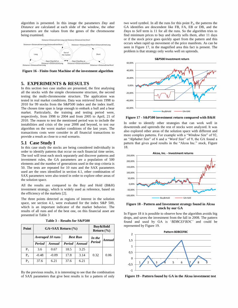
5. EXPERIMENTS & RESULTS In this section two case studies are presented, the first analysing

all the stocks with the simple chromosome structure, the second

testing the multi-chromosome structure. The application was

tested in real market conditions. Data was retrieved from 1998 to

2010 for 99 stocks from the S&P500 index and the index itself.

The chosen time span is large enough to embark a bull and a bear

market. Particularly, the training and testing period were,

respectively, from 1998 to 2004 and from 2005 to April, 21 of

2010. The reason to test the mentioned period was to include the

instabilities and crisis of the year 2008 and beyond, to test our

algorithm on the worst market conditions of the last years. The

transactions costs were consider in all financial transactions to

provide a result as close to a real scenario.

5.1 Case Study I In this case study the stocks are being considered individually in

order to identify patterns that occur on each financial time series.

The tool will treat each stock separately and discover patterns and

investment rules, the GA parameters are a population of 500

elements and the number of generations used in the stop criteria is

50. The tests are repeated for 10 runs and the SAX parameters

used are the ones identified in section 4.1, other combination of

SAX parameters were also tested in order to explore other areas of

the solution space.

All the results are compared to the Buy and Hold (B&H)

investment strategy, which is widely used as reference, based on

the efficiency of the markets [2].

The three points detected as regions of interest in the solution

space, see section 4.1, were evaluated for the index S&P 500,

which is an important indicator of the market behavior. The

results of all runs and of the best one, on this financial asset are

presented in Table 3

Table 3 – Results for S&P500

Point GA+SAX Return (%) Buy&Hold

Return (%)

Averaged 10 runs Best Run In the

Period Annual

Period Annual Period Annual

P1 3.6 0.67 18.5 3.25

0.32 0.06 P2 -0.48 -0.09 17.8 3.14

P3 37.6 6.21 37.6 6.21

By the previous results, it is interesting to see that the combination

of SAX parameters that give best results is for a pattern of only

two word symbol. In all the runs for this point P3, the patterns the

GA identifies are descendent like FB, FA, EB or DB, and the

Days to Sell term is 11 for all the runs. So the algorithm tries to

find minimum prices to buy and shortly sells them, after 11 days

or if the stock price goes quickly apart from the pattern and this

occurs when rapid up movement of the price manifests. As can be

seen in Figure 17, in the magnified area this fact is present. The

problem is that strategy only works well on uptrends.

Figure 17 - S&P500 investment return compared with B&H

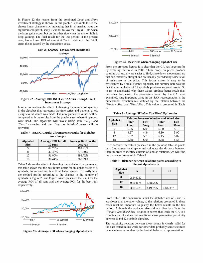
In order to identify other strategies that can work well in

downtrends and uptrends the rest of stocks were analyzed. It was

also explored other areas of the solution space with different and

more complex patterns. For example with a “Window Size” of 92,

an “Alphabet Size” of 6 and a “Word Size” of 9, the GA found a

pattern that gives good results in the “Alcoa Inc.” stock, Figure

18.

Figure 18 - Pattern and Investment strategy found in Alcoa

stock by our GA

In Figure 18 it is possible to observe how the algorithm avoids big

drops, and saves the investment from the fall in 2008. The pattern

found and used by GA is ‘BDBCEFBDC’ and could be

represented by Figure 19.

Figure 19 - Pattern found by GA in the Alcoa investment test

-60,00%

-40,00%

-20,00%

0,00%

20,00%

40,00%

60,00%

S&P500 Investment return

Buy&Hold GA+SAX

-100,00%

-50,00%

0,00%

50,00%

100,00%

150,00%

200,00%

250,00% Alcoa, Inc. - Investment returns

Buy&Hold GA+SAX

-1

-0,5

0

0,5

1

1,5

2

1 2 3 4 5 6 7 8 9

Pattern BDBCEFBC

The results presented in Table 4 are the average earnings of the

investment strategies for the best chromosomes of all the stocks,

compared to the B&H.

Table 4 - Average return of all stocks investment strategies.

SAX Parameters GA+SAX Return

(%)

Buy&Hold

Return (%)

n a w Period Annual Period Annual

10 7 2 69.30 10.44

48.80 7.79

10 18 3 117.82 15.82

17 13 4 115.18 15.56

60 13 4 113.28 15.36

92 6 9 120.49 16.09

104 6 8 115.24 15.56

128 7 8 111.43 15.17

136 5 12 122.39 16.28

From Table 4 it is possible to verify that areas of SAX parameters,

others than the detected in section 4.1, are valid and prove to get

better results. As expected the pattern search for a two symbol

word gave the worst results on average.

Another study, concerning the measure types used to determine

the degree of similitude between the time series and the pattern,

was made. To find which distance measure is used with better

result in the investment strategies were analyzed only the best

runs of the GA, the results are presented in Table 5.

Table 5 - Measure type analysis

Measure Type Occurrences

MINDIST (Eq.3) 97 69.8%

ALPHAB. DIST. (Eq.4) 42 30.2%

From Table 5 is possible to verify that the method chosen by the

GA to find the best investment strategy was the distance measure

defined by the SAX method, which is a lower bounding of the

Euclidian distance of the time series and the pattern. The sum of

occurrences in the result table is bigger than 100, the number of

stocks, because more than one run has the same result.

5.2 Case Study II Since this multi-chromosome approach allows two investment

strategies, Long and Short, several combinations have been tried

with these parameters, in some cases it was allowed both in others

just one of them was allowed. Another parameter that was subject

to changes was the activation or not of the ‘Days to Sell/Days to

Buy’ gene. For all the major tests the alphabet size was 8 symbols,

but some tests were made using other values, to evaluate how this

parameter affects the performance. Like in previous tests 10 runs

were made.

For the GA parameters a population of 200 individuals and 50

generations were used.

As was previously referred, several combinations with strategies

Long and Short were tested, as well the activation of ‘Sell/Buy

Day’ gene the results of this test are presented in Table 6. Where

it is clear that the best results are obtained when the ‘Days to

Sell/Buy’ gene is activated. The best investment strategy is when

the two trading methods are enabled, Long and Short, this is

because in this case the algorithm could invest and profit in bear

and bull market. The poor results are obtained when applying only

Short, and are caused by the fact that the algorithm was trained on

period that was indicated to Long investment strategy, so only

when the algorithm gets to the 2008 crash it can make some

profit, this can be seen in Figure 20.

Table 6 - Multi-Chromosome Structure Results - Changing

Investment Strategies and ‘Days to Sell/Buy’ Gene activation

‘Days to

Buy/Sell’

Gene

Long

Strategy

Short

Strategy

Average

ROI for

all 10

runs

Average

ROI for

the best

run

Enable Enable Enable 42.35% 276.80%

Enable Enable Disable 30.43% 113.52%

Enable Disable Enable 0.84% 83.86%

Disable Enable Enable 23.00% 179.61%

Disable Enable Disable 21.34% 108.46%

Disable Disable Enable -9.69% 52.74%

Figure 20 - Average ROI B&H vs. SAX/GA - Short

Investment Strategy

In Figure 21 the return of the Long investment strategy is shown.

In this figure is possible to observe that in the left side of the

graphic the algorithm follows the B&H but with not so much

profit, this is caused by the transaction cost that exists when the

algorithm exits or enters the market. In the 2008 crash the

algorithm does not drop as much as the B&H, in fact it recovers,

but after again it goes apart from the B&H caused by the

transaction costs. So the gains in this algorithm come from

avoiding big drops.

Figure 21 - Average ROI B&H vs. SAX/GA - Long Investment

Strategy

-20,00%

0,00%

20,00%

40,00%

60,00%

B&H vs. SAX/GA - Short Investment strategy

B&H SAX/GA - Short

-20,00%

0,00%

20,00%

40,00%

60,00%

B&H vs. SAX/GA - Long Investment strategy

B&H SAX/GA - Long

In Figure 22 the results from the combined Long and Short

investment strategy is shown. In this graphic is possible to see the

almost linear characteristic indicating that in all market types the

algorithm can profit, sadly it cannot follow the Buy & Hold when

the large gains occur, but on the other side when the market falls it

keep gaining. The final result for the test period, in the present

case, has a lower ROI of almost 6.5% in relation to the B&H,

again this is caused by the transaction costs.

Figure 22 - Average ROI B&H vs. SAX/GA - Long&Short

Investment Strategy

In order to evaluate the effect of changing the number of symbols

in the alphabet that represents the time series and patterns, a test

using several values was made. The new parameter values will be

compared with the results from the previous test where 8 symbols

were used. The algorithm will invest using both ‘Long’ and

‘Short’ strategies and the ‘Days to Sell/Buy’ genes will be

activated.

Table 7 - SAX/GA Multi-Chromosome results for alphabet

size changes

Alphabet

Size

Average ROI for all

10 runs

Average ROI for the

best run

5 62.76% 482.41%

8 42.35% 276.80%

12 51.00% 393.72%

18 36.44% 262.89% Table 7 shows the effect of changing the alphabet size parameter,

this table shows that the best return occur for an alphabet size of 5

symbols, the second best is a 12 alphabet symbol. To verify how

the method profits according to the changes in the number of

symbols in Figure 23 and Figure 24 are presented the result for the

average ROI of all runs and the average ROI for the best runs

respectively.

Figure 23 - Average ROI when changing alphabet size

Figure 24 - Best runs when changing alphabet size

From the previous figures it is clear that the GA has large profits

by avoiding the crash in 2008. These drops on prices produce

patterns that usually are easier to find, since down movements are

fast and relatively straight and are usually preceded by some level

of resistance in the price. This factor makes it easy to be

represented by a small symbol alphabet. The surprise here was the

fact that an alphabet of 12 symbols produces so good results. So

to try to understand why these values produce better result than

the other two cases, the parameters found by the GA were

examined. One important value in the SAX representation is the

dimensional reduction rate defined by the relation between the

‘Window Size’ and ’Word Size’. This value is presented in Table

8.

Table 8 - Average ‘Window Size/Word Size’ results

Alphabet

Size

Relation between Window and Word size

Enter

Long

Exit

Long

Enter

Short

Exit

Short

5 5.55 6.03 5.80 5.10

8 4.57 4.24 6.30 5.90

12 5.32 5.75 6.15 5.07

18 5.38 6.05 8.78 5.53 If we consider the values presented in the previous table as points

in a four dimensional space and calculate the distance between

them in order to identify clusters of similar relations, we will find

the distances presented in Table 9

Table 9 - Distance between relations points according to

diferent alphabet size

Alphabet

Size 5 8 12

8 2.248222

12 0.504678 1.885206

18 3.015725 3.196795 2.687397

From Table 9 the conclusion is that the alphabet size of 5 and 12

are closer than the other values, so the relations presented in these

cases must be important to justify the better results in the test

period. Although the alphabet size did not directly affects the

‘Window Size/Word Size’ relation it seems that leads the GA to a

combination of values that results on close parameters proximity

between 5 and 12 symbols alphabet.

The proximity relation between those points is clearly valid for

the data tested in this work, for other data probably some test must

be made in order to identify the best alphabet size representation.

-20,00%

0,00%

20,00%

40,00%

60,00%

B&H vs. SAX/GA - Long&Short Investment strategy

B&H SAX/GA - Long&Short

-20,00%

30,00%

80,00%

130,00%

B&H 18 Symbol 12 Symbol

8 Symbol 5 Symbol

-20,00%

480,00%

980,00%

B&H 18 Symbol 12 Symbol

8 Symbol 5 Symbol

6. CONCLUSIONS The methodology that was presented here has great potential on

investment markets. The GA proves its adaptability to find good

solutions to the problem at hand. The flexible chromosome

structure adopted allows finding several different patterns with

different dimensions. This was possible thanks to the use of the

SAX representation that is capable of dimensional reduction of

the time series and still maintains the principal characteristics of

the financial data.

From the two case studies it was identified that the investment

method to apply is the one with the multi-chromosome structure,

this was in part expected since this approach allows applying

several investment strategies and profiting from bear and bull

market conditions.

A future evolution of this study is to include all the SAX

parameters in the GA, to identify the best ones to represent

financial data. In order to improve the results and also reduce the

overfitting effect a change on the training/testing process will be

made, the present approach uses a large fixed training period

followed by the testing period. To improve the method a sliding

window strategy will be implemented. This will allow the testing

period to be closer to the training reality.

7. REFERENCES [1] Agrawal, R., Faloutsos, C., and Swami, A. 1993. Efficient

Similarity Search in Sequence Databases. In Proceedings of

the 4th International Conference on Foundations of Data

Organization and Algorithms (FODO '93). 69-84.

[2] Bernstein , P.L. 1999. A new look at the efficient market

hypothesis. The Journal of Portfolio Management 25, 2, 1-2,

(Winter 1999).

[3] Bulkowski, T. N. 2005. Encyclopedia of Chart Patterns, 2nd

Edition. John Wiley and Sons.

[4] Fu, T., Chung, K.F., Kwok, K., and Ng, C. 2008. Stock time

series visualization based on data point importance. Eng.

Appl. Artif. Intell. 21, 8 (Dec. 2008), 1217-1232. DOI=

http://dx.doi.org/10.1016/j.engappai.2008.01.005.

[5] Goldin, D. and Kanellakis, P. 1995. On Similarity Queries

for Time-Series Data: Constraint Specification and

Implementation. In Proceedings of the First International

Conference on Principles and Practice of Constraint

Programming (CP '95), 137-153.

[6] Hua-Ning, H. 2010. Short-term forecasting of stock price

based on genetic-neural network. In Natural Computation

(ICNC), 2010 Sixth International Conference on (10-12 Aug.

2010), 4, 1838-1841.

[7] Keogh, E., Chakrabarti, K., Pazzani, M. and Mehrotra, S.

2001. Dimensionality reduction for fast similarity search in

large time series databases. Journal of Knowledge and

Information Systems, 3, 3, 263–286. (Aug. 2001). DOI=

http://dx.doi.org/10.1007/PL00011669.

[8] Krause, A. 2011. Performance of evolving trading strategies

with different discount factors. In Congress on Evolutionary

Computation (CEC), 2011 IEEE, (5-8 Jun. 2011), 186-191.

DOI= http://dx.doi.org/10.1109/CEC.2011.5949617.

[9] Lei Wang and Qiang Wang. 2011. Stock Market Prediction

Using Artificial Neural Networks Based on HLP. In

Proceedings of the 2011 Third International Conference on

Intelligent Human-Machine Systems and Cybernetics -

Volume 01 (IHMSC '11), 1, 116-119.

DOI=http://dx.doi.org/10.1109/IHMSC.2011.34.

[10] Lin, J., Keogh, E., Lonardi, S. and Chiu, B. 2003. A

symbolic representation of time series, with implications for

streaming algorithms. In Proceedings of the 8th ACM

SIGMOD workshop on Research issues in data mining and

knowledge discovery (DMKD '03). ACM, New York, NY,

USA, 2-11. DOI=http://doi.acm.org/10.1145/882082.882086.

[11] Lin, J., Keogh, E., Lonardi, S. and Patel, P. 2002. Finding

Motifs in Time Series, Proceedings of the 2nd Workshop n

Temporal Data Mining (2002), 53-68.

[12] Matsui, K. and Sato, H. 2010. Neighborhood evaluation in

acquiring stock trading strategy using genetic algorithms. In

Soft Computing and Pattern Recognition (SoCPaR), 2010

International Conference. (7-10 Dec. 2010), 369-372, DOI=

10.1109/SOCPAR.2010.5686733.

[13] Ng, W.W.Y., Xue-Ling Liang, Chan, P.P.K. and Yeung, D.S.

2011. Stock investment decision support for Hong Kong

market using RBFNN based candlestick models. In Machine

Learning and Cybernetics (ICMLC), 2011 International

Conference. 2, (10-13 Jul. 2011), 538-543, DOI=

10.1109/ICMLC.2011.6016839.

[14] Parque, V., Mabu, S. and Hirasawa, K. 2010. Enhancing

global portfolio optimization using genetic network

programming. In SICE Proceedings of Annual Conference

2010. (18-21 Aug. 2010), 3078-3083.

[15] Parracho, P., Neves, R. and Horta, N. 2011. Trading with

optimized uptrend and downtrend pattern templates using a

genetic algorithm kernel, In Congress on Evolutionary

Computation (CEC), 2011 IEEE, (5-8 Jun. 2011), 1895-

1901. DOI=10.1109/CEC.2011.5949846.

[16] Pinto, J., Neves, R. F. and Horta, N. 2011. Fitness function

evaluation for MA trading strategies based on genetic

algorithms. In Proceedings of the 13th annual conference

companion on Genetic and evolutionary computation

(GECCO '11). ACM, New York, NY, USA, 819-820. DOI=

http://doi.acm.org/10.1145/2001858.2002105.

[17] Tahersima, H., Tahersima, M., Fesharaki, M. and Hamedi, N.

2011. Forecasting Stock Exchange Movements Using Neural

Networks: A Case Study. In Proceedings of the 2011

International Conference on Future Computer Sciences and

Application (ICFCSA '11). IEEE Computer Society,

Washington, DC, USA, 123-126. DOI=

http://dx.doi.org/10.1109/ICFCSA.2011.35.

[18] Zhijun, F., Guihua, L., Fengchang, F. and Shuai Li 2010.

Stock Forecast Method Based on Wavelet Modulus Maxima

and Kalman Filter. In Proceedings of the 2010 International

Conference on Management of e-Commerce and e-

Government (ICMECG '10). IEEE Computer Society,

Washington, DC, USA, 50-53. DOI=

http://dx.doi.org/10.1109/ICMeCG.2010.19.

PATTERN DISCOVERY - A SAX-GA Based Investment Strategy

Documents

Transcript of PATTERN DISCOVERY - A SAX-GA Based Investment Strategy