https://doi.org/10.1007/s10584-021-03071-7

WEATHER ATTRIBUTION

Pathways and pitfalls in extreme event attribution

Geert Jan van Oldenborgh1 ·Karin van der Wiel1 · Sarah Kew1 ·Sjoukje Philip1 · Friederike Otto2 ·Robert Vautard3 ·Andrew King4 ·Fraser Lott5 · Julie Arrighi6 ·Roop Singh6 ·Maarten van Aalst6,7

Received: 6 April 2020 / Accepted: 16 March 2021© The Author(s) 2021

AbstractThe last few years have seen an explosion of interest in extreme event attribution, the sci-ence of estimating the influence of human activities or other factors on the probability andother characteristics of an observed extreme weather or climate event. This is driven bypublic interest, but also has practical applications in decision-making after the event and forraising awareness of current and future climate change impacts. The World Weather Attri-bution (WWA) collaboration has over the last 5 years developed a methodology to answerthese questions in a scientifically rigorous way in the immediate wake of the event whenthe information is most in demand. This methodology has been developed in the practiceof investigating the role of climate change in two dozen extreme events world-wide. In thispaper, we highlight the lessons learned through this experience. The methodology itself isdocumented in a more extensive companion paper. It covers all steps in the attribution pro-cess: the event choice and definition, collecting and assessing observations and estimatingprobability and trends from these, climate model evaluation, estimating modelled hazardtrends and their significance, synthesis of the attribution of the hazard, assessment of trendsin vulnerability and exposure, and communication. Here, we discuss how each of these stepsentails choices that may affect the results, the common problems that can occur and howrobust conclusions can (or cannot) be derived from the analysis. Some of these develop-ments also apply to other attribution methodologies and indeed to other problems in climatescience.

Geert Jan van Oldenborgholdenborgh@knmi.nl

1 KNMI, De Bilt, Netherlands2 Environmental Change Institute, University of Oxford, Oxford, UK3 LSCE/IPSL, laboratoire CEA/CNRS/UVSQ, 91191 Gif sur Yvette Cedex, France4 School of Earth Sciences, University of Melbourne, Melbourne 3010, Australia5 Met Office Hadley Centre, Exeter, UK6 Red Cross Red Crescent Climate Centre, The Hague, Netherlands7 ITC, University of Twente, Enschede, Netherlands

Climatic Change (2021) 166: 13

/ Published online: 10 May 2021

Keywords Extreme event attribution · Extreme weather · Climate change · Detection andattribution

1 Introduction

Nowadays, whenever an extreme weather or climate event occurs, the question inevitablyarises whether it was caused by climate change or, more precisely, by the influence ofhuman activities on climate. The interpretation of this question hinges on the meaning ofthe word ‘caused’: just as in the connection between smoking and lung cancer, the influ-ence of anthropogenic climate change on extreme events is inherently probabilistic. Allen(2003) proposed that a related question could be answered: how has climate change affectedthe probability of this extreme event occurring? The process to answer these questions isreferred to as ‘extreme event attribution’ and also includes attributing the change due toanthropogenic climate change in other characteristics, such as the intensity of the event.

Since its initiation in 2015, the World Weather Attribution (WWA), an international col-laboration of climate scientists, has sought to provide a rapid response to this question in ascientifically rigorous way for many extreme events with large impacts around the world.The motivation is that, by providing scientifically sound answers when the informationis most in demand, within a few weeks after the event. It has three uses: answering thequestions from the public, informing the adaptation after the extreme event (e.g. Sippelet al. 2015; Singh et al. 2019) and increasing the ‘immediacy’ of climate change, therebyincreasing support for mitigation (e.g. Wallace, 2012 ). Because rapid studies are necessarilyrestricted to types of events for which we have experience, WWA has also conducted slowattribution studies to build up experience for other extremes. The methodology developedby WWA for both types is documented in a companion paper (Philip et al. 2020a), whilsthere we highlight the lessons learned along the way. These are more general and also applyto other extreme event attribution methodologies and other fields in climate projections thatseek to predict or project properties of extreme weather and climate events.

Despite the extreme event attribution branch of climate science only originating in thetwenty-first century, there is already a wealth of literature on it. An early overview, reportingexperiences similar to ours is Stott et al. (2013). The assessment of the National Academiesof Sciences (2016) gives a thorough evaluation of the methods of extreme event attribution,which we have applied and expanded in the WWA methodology. Recent reviews of emerg-ing methods and differences in framing (the scientific interpretation of the question that willbe answered) and event definition (the scientific definition of the extreme event, specifyingits spatial-temporal scales, magnitude and/or other characteristics) were given by Stott et al.(2016), Easterling et al. (2016), and Otto (2017). While the term ‘event attribution’ is alsoused in studies focussing mainly on the evolution and predictability of an event due to allexternal factors (e.g. Hoerling et al. 2013a), we here apply it to the probabilistic approachsuggested by Allen (2003) that only focuses on anthropogenic climate change, which isalso the methodology applied in recent rapid attribution studies. The basic building blockshave been refined since the first study of the 2003 European heat wave (Stott et al. 2004).Originally, event attribution was based on the frequency of the class of events in a modelof the factual world in which we live, compared to the frequency in a counterfactual worldwithout anthropogenic emissions of greenhouse gases and aerosols. Later, it was realisedthat climate change is now so strong that this attribution result from model data can oftenbe compared to the observed trend over a long time interval (van Oldenborgh 2007). Notethat the framing of the attribution question for observations is not exactly comparable to

Climatic Change (2021) 166: 13Page 2 of 2713

that for models: even when human-induced climate change is the strongest observed driverof change, it is not the only one as it often is in model experiments. This is similar to thedifference between Bindoff et al. (2013), who consider only anthropogenic climate change,and Cramer et al. (2014), who consider all changes in the climate.

We, the authors, collectively and individually have conducted many event attributionanalyses over recent years, often in the World Weather Attribution (WWA) collabora-tion that aims to do scientifically defensible attribution on short time scales after eventswith large impacts (www.worldweatherattribution.org). This paper follows the eight-stepprocedure has emerged from our experience:

1. analysis trigger,2. event definition,3. observational trend analysis,4. climate model evaluation,5. climate model analysis,6. hazard synthesis,7. analysis of trends in vulnerability and exposure, and8. communication.

The final result usually takes the form of a probability ratio (PR): ‘the event has becomeX times more/less likely due to climate change with a 95% confidence interval of Y toZ’, often combined with ‘other factors such as . . . have also influenced the impact of thisextreme event’. Similar statements can be made about other properties of the extreme event,such as the intensity: ‘the heat wave has become T (T1 to T2) degrees warmer due to climatechange.’ We discuss the pathways through the steps leading to such statements in turn,emphasising the pitfalls we have encountered.

2 Analysis trigger

First, a choice has to be made which events to analyse. The Earth is so large that extremeweather events happen somewhere almost every day. Given finite resources, a method isneeded to choose which ones to attribute. In WWA, we choose to focus on extremes thatimpact people, a threshold could for example be the number of casualties or people affected.This implies considering more events in less developed regions where extreme weatherhas large impacts, and less in developed regions with numerically smaller impacts butmore news coverage (Otto et al. 2020). Alternatively, meteorological (near-)records with-out notable impacts on humans also sometimes lead to public debate of the role of climatechange, warranting scientific evidence. Stakeholders such as funding organisations oftenprioritise local events, so that small events locally can often be considered as importantas bigger events elsewhere. This implies that at this stage, the vulnerability and exposurecontext as well as the communication plans play a large role.

Impact-based thresholds need careful consideration. An economic impact–based thresh-old will focus event analysis on higher-income countries, and a population-based thresholdwill focus event analysis on densely populated regions such as in India or China, or affect-ing major cities. In line with our goal of attributing impactful events, the WWA team hasdeveloped a series of thresholds which combine meteorological extremes with extreme eco-nomic loss or extreme loss of life, the latter two both in absolute terms as well as percent losswithin a national boundary. The current criteria are ≥ 100 deaths or ≥ 1, 000, 000 people

Climatic Change (2021) 166: 13 Page 3 of 27 13

affected or ≥ 50% of total population affected. For heat and cold waves, the true impactis very hard to estimate in real time so we use more indirect measures. In practice, theseare typically the events that the International Federation of Red Cross and Red CrescentSocieties do international appeals for.

Even if the selection criteria would be totally objective, one cannot interpret the set ofextreme event attribution statements as an indicator of climate change because events thatbecome less extreme will be underrepresented in the analyses (Stott et al. 2013). As anexample, a spring flood due to snowmelt has not happened recently in England, but did occuroccasionally in the nineteenth and early twentieth centuries (e.g. 1947). Hence, there areno attribution studies that show that these events have become much less common (Bindoffet al. 2013) and an aggregate of individual attribution studies will leave out this negativetrend. To study global changes in extremes systematically, other methods are needed.

In practice, the situation is worse, because the question on the influence of climate changeis posed most often when a positive connection is suspected. The result of this bias and theselection bias discussed above is that even while each event attribution study strives to givean unbiased estimate of the influence of climate change on the extreme event, a set of eventattribution studies does not give an unbiased estimate of the influence on extreme events ingeneral. Therefore, while cataloguing extreme event analyses is useful, synthesising resultsacross event attribution studies is problematic (Stott et al. 2013).

In addition to these issues encountered when considering events that we would like toanalyse, we acknowledge there are additional practical issues that place further restrictionson which events can currently be readily analysed. It must be possible for models to rep-resent the event and if impact (hydrological) modelling is required, the time available mustallow for it. For example, long runs from convection-permitting models need to becomeavailable before it is possible to conduct a rapid analysis on convective rainfall extremes.Further examples of event types that currently pose a challenge are listed in the nextsection.

3 Event definition

Once an extreme event has been selected for analysis, our next step is to define it quan-titatively. This step has turned out to be one of the most problematic ones in eventattribution, both on theoretical and practical grounds. The results of the attribution studycan depend strongly on this definition, so the choice needs to be communicated clearly. Itis also influenced by pragmatic factors like observational and model data availability andreliability.

There are three possible goals for an event attribution analysis that lead to differentrequirements on the event definition. The first is the traditional Detection and Attributiongoal of identifying the index that maximises the anthropogenic contribution to test for anexternal forcing signal (Bindoff et al. 2013), which calls for averages over large areas andtime scales. However, these scales are often not relevant for the impacts that really affectpeople. In those cases, this event definition does not meet our goal to be relevant for adap-tation and only addresses the need for mitigation in an abstract way. These goals usuallyrequire a more local event definition, so we do not pursue this here. The second goal is themeteorological extreme event definition, choosing an index that maximises the return timeof the event (Cattiaux and Ribes 2018). This often also increases the signal-to-noise ratio.The third is to consider how the event impacts on human society and ecosystems and iden-tify an index that is best linked to these impacts. As these systems have often developed to

Climatic Change (2021) 166: 13Page 4 of 2713

cope with relatively common events but are vulnerable to very rare events, all definitionsmay overlap. As in the trigger phase, the communication plan also gives input to the eventdefinition, noting carefully what questions are being asked and how we can map these onphysical variables that we can attempt to attribute. These can be meteorological variables,but we also include other variables such as hydrological variables and other physical impactmodels.

The answer also depends on the ‘framing’: how the attribution question to be answeredwill be posed scientifically. We choose to use a ‘class-based’ definition, considering allevents of a similar magnitude or more extreme on some linear scale. This class-based defi-nition is well-defined as the probability of these events can be determined in principle fromcounting occurrences in the present and past climates, or model representations of these.Within the class-based framing, one can choose which factors to vary and which to keepconstant. We generally choose the most general framing, keeping only non-climate factorsexcept land use constant.

Alternative framings restrict the class of events by prescribing boundary conditions thatwere present, from the phase of El Nino to the particular event in all its details (Otto et al.2015a; Hannart et al. 2016; Otto et al. 2016; Stott et al. 2017). Because each event is unique(van den Dool 1994), the latter ‘individual event’ interpretation is harder to define: it hasa probability very close to zero and the results depend on how the extreme event is sep-arated from the large-scale circulation that is prescribed. Using this definition also risksgiving a non-robust and hence unusable result due to selection bias and the chaotic natureof the atmosphere: the conditions were optimal to produce the extreme event in the cur-rent climate and any perturbation, including the shift to a colder climate that is done in theattribution exercise, can decrease the probability of such an event, sometimes dramatically(Cipullo 2013; Shepherd 2016). Such a decrease then does not describe the effect of climatechange on the event but the effect of changing boundary conditions away from the optimalconditions. We therefore use event definitions at the inclusive end of the spectrum, eitherincluding all climate variables or prescribing only SST. The event being attributed only setsthe threshold, so the procedure can also be followed for past or fictitious events.

It should also be noted that many hazards result in impacts through a variety of factors.One example is a flood, triggered by extreme rainfall in a river basin. In addition, how-ever, the impact may also be affected by prior rainfall, snowmelt, dams or storage basins. Ifhydrological data are available (observations and model output), we can include these fac-tors. In addition, the vulnerability and exposure of the population or infrastructure to thehazard also determines the total impact and thus are also taken into consideration for theevent definition. At the moment, quantitative attribution of impacts of anthropogenic cli-mate change is work in progress, although a number of such studies have been published,e.g. Schaller et al. (2016) and Mitchell et al. (2016). They are significantly more challeng-ing as the vulnerability and exposure vary with time, behaviour and policies. It is discussedfurther in Section 8.

As noted above, we use a class-based definition of extreme events attribution, i.e.we consider the change in probability of an event that is as extreme or worse than theobserved current one, p(X ≥ x0) in two climates. This is described by the probability ratioPR = p1/p0, with p1 the probability in the current climate and p0 the probability in thecounterfactual climate without climate change or the pre-industrial climate (often approxi-mated by late nineteenth century climate). The univariate measurable, physical variable X

measures the magnitude of the event. Compound events in meteorological variables can beanalysed the same way using a physical impact model to compute a one-dimensional impactvariable. As an example, moderate rainfall and moderate wind causing extreme water levels

Climatic Change (2021) 166: 13 Page 5 of 27 13

in the North of the Netherlands (van den Hurk et al. 2015) can be analysed using a modelof water level. Similarly, drought and heat can be combined onto a forest fire risk index,which lends itself to the class-based event event definition (Kirchmeier-Young et al. 2017;Krikken et al. 2019; van Oldenborgh et al. 2020)

The definition next includes the spatial and temporal properties of the variable: the aver-age or maximum over a region and timescale, possibly restricted to a season. As an example,an event definition would be the April–June maximum of 3-day averaged rainfall over theSeine basin, with the threshold given by the 2016 flooding event (Philip et al. 2018a).The temporal/spatial averaging has a large influence on the outcomes, as large scales oftenreduce the natural variability without affecting the trend much, thus increasing the Proba-bility Ratio (Fischer et al. 2013; Angelil et al. 2014; Uhe et al. 2016; Angelil et al. 2018;Leach et al. 2020). Describing the 2003 European heat wave by the temperature averagedover Europe and June–August (Stott et al. 2004) gives higher probability ratios than con-centrating on the hottest 10 days in a few specific locations, which gave the largest impacts(Mitchell et al. 2016). We reduce the range of possible outcomes by demanding that theevent definition should be as close as possible to the question asked by or on behalf of peopleaffected by the extreme, while being representable by the models. Additional informationfrom local experts is essential. For instance, for the event definition used in the study of theEthiopian drought in 2015 (Philip et al. 2018b), the northern boundary of the spatial eventdefinition, a rectangular box, was originally taken to be at 14 N, but after discussions withlocal experts, who informed us about the influence of the Red Sea in the North, we changedthe northern boundary to 13 N.

Choosing an average over the area impacted by the event has one unfortunate side effect:it automatically makes the event very rare, as other similar events will in general be offsetin space and only partially reflected in the average. A more realistic estimate of the rarityof the event can be obtained by considering a field analysis: the probability of a similarevent anywhere in a homogeneous area. For instance, we found that 3-day averaged stationprecipitation as high as observed in Houston during Hurricane Harvey had a return time ofmore than 9000 years, but the probability of such an event occurring anywhere on the USGulf Coast is roughly one in 800 years (van Oldenborgh et al. 2017).

For heat, a common index is the highest maximum temperature of the year (TXx) rec-ommended by the Expert Team on Climate Change Detection and Indices (ETCCDI). Amajor impact of heat is on health, mortality increases strongly during heat waves (Fieldet al. 2012). According to the impact literature, TXx is a useful measure when the vulnera-ble population is outdoors, e.g. in India (e.g. Nag et al., 2009 ) and accordingly, this is themeasure we used in our Indian heat wave study (van Oldenborgh et al. 2018). In Europe,there is evidence that longer heat waves are more dangerous (D’Ippoliti et al. 2010), so thatthe maximum of 3-day average maximum temperatures, TX3x, may be a better indicator.We have also used the 3-day average daily mean temperature, TG3x, which correlates aswell with impacts as the daily maximum and is less sensitive to small-scale factors affectingthe observations.

There are many ways to define a heat index that is better correlated to health impacts thantemperature. The Universal Thermal Comfort Index (UTCI) consists of a physical model ofhow humans dissipate heat (McGregor 2012). However, this necessitates the specificationof the clothing style and skin colour, which makes the results less than universally applica-ble. From a practical point of view, it requires wind speed and radiation observations, whichare often lacking or unreliable. A useful compromise is the wet bulb temperature (van Old-enborgh et al. 2018; Li et al. 2020), which is a physical variable based on temperature andhumidity that is closely related to the possibility of cooling through perspiration..

Climatic Change (2021) 166: 13Page 6 of 2713

Cold extremes can be described similarly to heat extremes. The annual minima of thedaily minimum, maximum and mean temperature are often useful ETCCDI measures. Formultiple-day events, such as the Eleven City Tour in the Netherlands, an averaging periodor, in this case an ice model, can represent the event best (Visser and Petersen 2009; de Vrieset al. 2012). Windchill factors giving a ‘feels like’ temperature have not yet been included inour attribution studies, due to the aforementioned problems of wind observations. Snowfalland snow depth also seem amenable to attribution studies, but only a handful of such studieshave been done up to now (e.g. Rupp et al. 2013; van Oldenborgh and de Vries 2018).

For high precipitation extremes, the main impact usually is flooding. This should be des-cribed by a hydrological model (e.g. Schaller et al., 2016 ), but precipitation averaged over therelevant river basin with a suitable time-averaging can often be used instead (Philip et al.2019). For in situ flooding, we can choose point observations as the main indicator, asthe time-averaging already implies larger spatial scales (e.g. van der Wiel et al. 2017; vanOldenborgh et al. 2017). A complicating factor is that human influence on flood risk isnot only through changes in atmospheric composition and land use but also via river basinmanagement, which often makes the attribution of floods rather than extreme precipitationmore difficult.

Droughts add additional degrees of complication. Meteorological drought, lack of rain,is easy to define as the low tail of a long-time scale averaged precipitation, from a season tomultiple years. Agricultural drought, lack of soil moisture, requires good soil modules in theclimate model or a separate hydrological model that includes effects of irrigation. A watershortage also requires including other human interventions in the water cycle. In practice,lack of rain is often chosen, with qualitative observations on other factors (e.g. Hoerlinget al. 2014; Otto et al. 2015b; Hauser et al. 2017; Otto et al. 2018a), although some studieshave attributed drought indices like the self-calibrating Palmer Drought Severity Index (e.g.Williams et al. 2015; Li et al. 2017) or soil moisture and potential evaporation (e.g. Kewet al. 2021 ).

There are many other types of events for which attribution studies are requested, forinstance wind storms, tornadoes, hurricanes, hail and freezing rain. Standard event defini-tions for these have as far as we know not yet been developed and long homogeneous timeseries and model output for these variables are often not readily available.

4 Observed probability and trend

The next step is to analyse the observations to establish the return time of the event andhow this has changed. This information is also needed to evaluate and bias-correct the cli-mate models later on, so in our methodology the availability of sufficient observations isa requirement to be able to do an attribution study. This causes problems in some parts ofthe world, where these are not (freely) available (Otto et al. 2020). Early attribution stud-ies relied solely on models. However, including observations is in our experience needed toinvestigate whether the climate models represent the real world well enough to be used inthis way, making the results more convincing when this is the case.

A long time series is needed that includes the event but goes back at least 50 years andpreferably more than 100 years. Observations are often less than perfect and care has to betaken to choose the most reliable dataset. As an example, Fig. 1 shows four estimates of the3-day averaged precipitation from Hurricane Harvey around Houston. The radar analysis isprobably the most reliable one, but is only available since 2005. The CPC gridded analysis

Climatic Change (2021) 166: 13 Page 7 of 27 13

ba

dc

Fig. 1 Observed maximum 3-day averaged rainfall over coastal Texas January–September 2017 (mm/dy).a GHCN-D v2 rain gauges, b CPC 25 km analysis, c NOAA calibrated radar (August 25–30 only) and dNASA GPM/IMERG satellite analysis. From van Oldenborgh et al. (2017)

only uses stations that report in real time and therefore underestimates the event. The satel-lite analysis diverges strongly from the others. Here, we chose the station data as the mostreliable dataset with a long time series, more than 100 years for many stations.

Due to the relatively small number of observed data points, some assumptions have tobe made to extract the maximum information from the time series. These assumptions canlater be checked in model data. They commonly are:

– the statistics are described by an extreme value distribution, for instance generalisedextreme value (GEV) function for block maxima or generalised Pareto distribution(GPD) for threshold exceedances; these depend on a position parameter μ or thresholdu, a scale parameter σ and a shape parameter ξ (sometimes other distributions, such asthe normal distribution, can be used),

– the distribution only shifts or scales with changes in smoothed global mean surfacetemperature (GMST) and does not change shape,

– global warming is the main factor affecting the extremes beyond year-to-year naturalvariability.

The first assumption can be checked by comparing the fitted distribution to the observed(or modelled) distribution, discrepancies are usually obvious. For temperature extremes,keeping the scale and shape parameters σ, ξ constant is often a good approximation. For

Climatic Change (2021) 166: 13Page 8 of 2713

precipitation and wind, we keep the dispersion parameter σ/μ and ξ constant, the indexflood assumption (Hanel et al. 2009). This assumption can usually also be checked in modeloutput. For many extremes, global warming is the main low-frequency cause of changes,but decadal variability, local aerosol forcing, irrigation and land surface changes may alsobe important factors. This will be checked later by comparing the results to those of cli-mate models that allow drivers to be separated. For instance, increasing irrigation stronglydepresses heat waves (Lobell et al. 2008; Puma and Cook 2010). In Europe, the strongdownward trend in observed wind storm intensity over land areas appears connected to theincrease in roughness (Vautard et al. 2019).

Often, the tail of the distribution is close to an exponential fall-off. If the change inintensity is close to independent of the magnitude, this implies that the probability ratio doesnot depend strongly on the magnitude of the event. In those common cases, the uncertaintyassociated with a preliminary estimation of the magnitude in a rapid attribution study doesnot influence the outcome much (Stott et al. 2004; Pall et al. 2011; Otto et al. 2018a; Philipet al. 2018a).

One exception is the distribution of the hottest temperature of the year, which typicallyappears to have an upper limit (ξ < 0). This limit increases with global warming. Anexample is shown in Fig. 2a, c (daily mean temperature at De Bilt, the Netherlands). Underthe assumption of constant shape of the distribution, this threshold in the climate of 1900was far below the observed value for 2018, so that formally the event would not have beenpossible then. However, this presumes the assumptions listed above are perfectly valid. Aswe cannot unequivocally show that this is the case, we prefer to state that the event wouldhave been extremely unlikely or virtually impossible.

a

18 20 22 24 26 28 30

-0.6 -0.4 -0.2 0 0.2 0.4 0.6 0.8 1

TGx

[Cel

sius

]

Smoothed global mean surface temperature [K]

Jan-Dec mean temperature De Bilt 1901:2017 b

0 50

100 150 200 250 300 350

-0.6 -0.4 -0.2 0 0.2 0.4 0.6 0.8 1

RX3

day

[mm

/day

]

Smoothed global mean surface temperature [K]

GHCN-D 13 stations

c

18

20

22

24

26

28

30

32

2 5 10 100 1000 10000

TGx

[Cel

sius

]

return period [yr]

Jan-Dec mean temperature De Bilt 1901:2017

GEV shift fit 1900GEV shift fit 2018

observed 2018

d

0

50

100

150

200

250

300

350

400

2 5 10 100 1000 10000

Rx3

day

[mm

/day

]

Return period [yr]

GHCN-D 13 stations

GEV scale fit 1900GEV scale fit 2017

Houston 2017

Fig. 2 a,c Highest daily mean temperature of the year at De Bilt, the Netherlands (homogenised), fitted to aGEV that shifts with the 4-year smoothed GMST. a As a function of GMST and c in the climates of 1900 and2018. b,d The same for the highest 3-day averaged precipitation along the US Gulf Coast fitted to a GEV thatscales with 4-year smoothed GMST. From climexp.knmi.nl, (b,d) also from van Oldenborgh et al. (2017)

Climatic Change (2021) 166: 13 Page 9 of 27 13

There are a few pitfalls to avoid in this analysis. In very incomplete time series, thevarying amount of missing data may produce spurious trends, because extremes will sim-ply not be recorded part of the time. For example, the maximum temperature series ofBikaner (India) has about 30% missing data in the 1970s but is almost complete in recentyears. This gives a spurious increase in the probability of observing an extreme of a factor100%/(100% − 30%) ≈ 1.4 that can be mistaken for an increase in the incidence of heatwaves (van Oldenborgh et al. 2018).

A related problem may be found in gridded analyses: if the distance between stationsis greater than the decorrelation scale of the extreme, the interpolation will depress theoccurrence of extremes, so that a lower station density will give fewer extremes. An extremeexample for this is given in Fig. 3, where the trend in May maximum temperature in India1975–2016 in the CRU TS 4.01 dataset is shown to be based on hardly any station data atall and therefore unreliable. In contrast, reanalyses can produce extremes between stationsand are based on many other sources of information. These are in principle therefore lesssusceptible to this problem than statistical analyses of observations. However, the quality ofreanalyses varies greatly by variable and region (Angelil et al. 2016). We found in this casethat the trends from a reanalysis in Fig. 3c are more reliable and in better agreement withstatistical analyses of the Indian Meteorological Department (van Oldenborgh et al. 2018).Similar problems in depressed extremes and spurious trends were found in an interpolatedprecipitation analysis of Australia (King et al. 2013).

There has been discussion on whether to include the event under study in the fit or not.We used not to do this to be conservative, but now realise that the event can be included ifthe event definition does not depend on the extreme event itself. If you analyse the CentralEngland Temperature every year, an extreme is drawn from the same distribution as the otheryears and can be included. However, if the event is defined to be as unlikely as possible, theextreme value is drawn from a different distribution and cannot be included.

We can sometimes increase the amount of data available by spatial pooling. Figure 2b, dshow a fit for precipitation data. In this case, the spatial extent of the events is smaller thanthe region over which they are very similar, so that we can make the additional assumptionthat the distribution of precipitation is the same for all stations. In this example, we showthe annual maximum of 3-day averaged precipitation (RX3day) at 13 GHCN-D stationswith more than 80 years of data and 1 apart along the US Gulf Coast. We verified that themean of RX3day is indeed similar throughout this region. Despite the applied 1 minimumseparation, the stations are still not independent, this is taken into account in the bootstrap

a b c

-2.5-2-1.5-1-0.50.511.522.5

1086420

-2.5-2-1.5-1-0.50.511.522.5

Fig. 3 a Trend of May maximum temperature in South Asia 1979–2016 in the CRU TS 4.01 dataset. bNumber of stations used to estimate the temperature at each grid point in CRU TS 4.01. c Trend of Maymaximum temperatures in the ERA5 reanalysis

Climatic Change (2021) 166: 13Page 10 of 2713

that is used to estimate the uncertainties by using a moving block technique (Efron andTibshirani 1998), giving about 1000 degrees of freedom. In spite of the diverse mechanismsfor extreme rainfall in this area, the observations are fitted well by one GEV. The 2018observation in Houston still requires a large extrapolation, so that we could only report alower bound of about 9000 years for the return time. The trend in this extreme, deducedfrom the fit to the less extreme events in more than a century of observations along the GulfCoast, is an increase of 18% (95% CI: 11–25%) in intensity (van Oldenborgh et al. 2017).

Whether trends can be detected in the observations depends strongly on the variable.Anthropogenic climate change is now strong enough that trends in heat extremes (e.g.Perkins et al., 2012) and short-duration precipitation extremes are usually detectable, forsmall-scale precipitation using spatial pooling (Westra et al. 2013; Vautard et al. 2015; Edenet al. 2016; Eden et al. 2018). Winter extremes are more variable but now also show signif-icant trends (Otto et al. 2018a; van Oldenborgh et al. 2019). We hardly ever find significanttrends in drought as the time scales are much longer and hence the number of independentevents in the observations lower. Drought is also usually only a problem when the anomalyis large relative to the mean, which usually implies that it is also large relative to the trend,so the signal-to-noise ratio is poor.

5 Model evaluation

In order to attribute the observed trend to different causes, notably global warming dueto anthropogenic emissions of greenhouse gases (partially counteracted by emissions ofaerosols), we have to use climate models. Observations can nowadays often give a trend,but cannot show what caused the trend. Approximations from simplified physics arguments,such as Clausius-Clapeyron scaling for extreme precipitation, have often been found to over-estimate (e.g. Hoerling et al., 2013b) or underestimate (e.g. Lenderink and van Meijgaard,2010) the modelled and observed trends, so we choose not to use these for the individualevents that we try to attribute.

However, before we can use these models, we have to evaluate whether they are fit forpurpose. We use the following three-step model evaluation.

1. Can the model in principle represent the extremes of interest?2. Are the statistics of the modeled extreme events compatible with the statistics of the

observed extremes?3. Is the meteorology driving these extremes realistic?

If a model ensemble fails, any of these tests it is not used in the event attribution analysis.Of course a ‘yes’ answer to these three questions is a necessary but not a sufficient condi-tion. These requirements do not prevent the model from being unable to represent the propersensitivity to human influence. However, in practice, this condition is hard to verify; hence,we rely on several methods and models. In our experience, the results of a single modelshould never be accepted at face value, as climate models have not been designed to rep-resent extremes well. Even when the extreme should be resolved numerically, the sub-gridscale parameterisations are often seen to fail under these extreme conditions. Trends canalso differ widely between different climate models (Hauser et al. 2017). If the variable ofinterest is a hydrological or other physical impact variable, it is also better to use multipleimpact models (Philip et al. 2020b; Kew et al. 2021).

The first step is rather trivial: it does not make sense to study extreme events in a modelthat does not have the resolution or does not include the physics to represent these. For

Climatic Change (2021) 166: 13 Page 11 of 27 13

instance, only models with a resolution of about 25 km can represent tropical cyclonessomewhat realistically (Murakami et al. 2015), so to attribute precipitation extremes onthe US Gulf Coast, we need these kinds of resolutions (van der Wiel et al. 2016; 2017).One-day summer precipitation extremes are usually from convective events, so one needsat least 12-km resolution and preferably non-hydrostatic models. Studying these events in200-km resolution, CMIP5 models do not make much sense (Kendon et al. 2014; Luu et al.2018). A work-around may be to use a two-step process in which coarser climate modelsrepresent the large-scale conditions conducive to extreme convection and a downscaling steptranslates these into actual extremes. However, this is contingent on a number of additionalassumptions and we have not yet attempted it. In contrast, midlatitude winter extremes arerepresented well by relatively coarse-resolution models (e.g. Otto et al., 2018a).

In order to compare the model output to observations, care has to be taken that theyare comparable. If the decorrelation scale of the event is larger than the model decorrela-tion scale (often grid size), point observations are comparable to grid values, because theextreme event will then cover multiple grid cells with similar values and in this area a pointobservation gives practically the same result as the nearest model grid point. In effect, thistranslates to our first model validation criterion. Another way to make observations andmodel output commensurate is to average both over a large area, such as precipitation overa river basin. We try not to interpolate data as this reduces extremes by definition.

A straightforward statistical evaluation entails fitting the tail of the distribution to anextreme value distribution and comparing the fit parameters to an equivalent fit to observeddata, preferably at the same spatial scale. Allowing for a bias correction, additive fortemperature and multiplicative for precipitation, this gives two or three checks:

– the scale parameter σ or the dispersion parameter σ/μ corresponding to the variabilityof the extremes (relative to the mean),

– the shape parameter ξ that indicates how fat or thin the tail is and– possibly the trend parameter.

The last check should only be used to invalidate a model if the discrepancy in trends isclearly due to a model deficiency, e.g. if other models reproduce the observed trends wellor if there is other evidence for a model limitation. Otherwise, it is better to keep the modeland evaluate the differences in the synthesis step (Section 7).

In our experience, for small-scale extremes, this often eliminates half the models as notrealistic enough. This is often due to problems in the sub-gridcell parameterisations of themodel. For instance, the MIROC-ESM family of models has unrealistic maximum tempera-tures in deserts well above 70 C. Another problem we found is that a large group of modelshave an apparent cut-off on precipitation of 200–300 mm/dy (van Oldenborgh et al. 2016),see Fig. 4. As climate models are developed further, there will likely be more emphasis onsimulating extremes correctly, which will potentially allow more models to be included inthe synthesis step.

There are other cases where the discrepancies are not unphysical but the climate modelresults are still not compatible with observations. Heat waves provide good examples. In theMediterranean, the scale parameter σ is about twice that in the observations in the modelsavailable to us with the required resolution, so that no model could be found that representsthe average maximum temperature over the area of the 2017 heat wave realistically (Kewet al. 2019). In France, the HadGEM3-A model does not reproduce the much less negativeshape parameter ξ that enables large heat waves (Vautard et al. 2018). The same holds formany other climate models (e.g. Vautard et al., 2020). As an example of wrong trends,

Climatic Change (2021) 166: 13Page 12 of 2713

a

0 50

100 150 200 250 300 350

2 5 10 100 1000 10000

Rx1

day

[mm

/day

]

return period [yr]

GEV scale fit 1879GEV scale fit 2006

observed 2006

b

0 50

100 150 200 250 300 350

2 5 10 100 1000 10000

Rx1

day

[mm

/day

]

return period [yr]

GEV scale fit 1879GEV scale fit 2006

observed 2006

c

0 50

100 150 200 250 300 350

2 5 10 100 1000 10000

Rx1

day

[mm

/day

]

return period [yr]

GEV scale fit 1960GEV scale fit 2006

observed 2006

Fig. 4 Return time plots of extreme rainfall in Chennai, India, in two CMIP5 climate models with ten ensem-ble members (CSIRO-Mk3.6.0 and CNRM-CM5) and an attribution model (HadGEM3-A N216) showing anunphysical cut-off in precipitation extremes. The horizontal line represents the city-wide average in Chennaion 1 December 2015 (van Oldenborgh et al. 2016)

Climatic Change (2021) 166: 13 Page 13 of 27 13

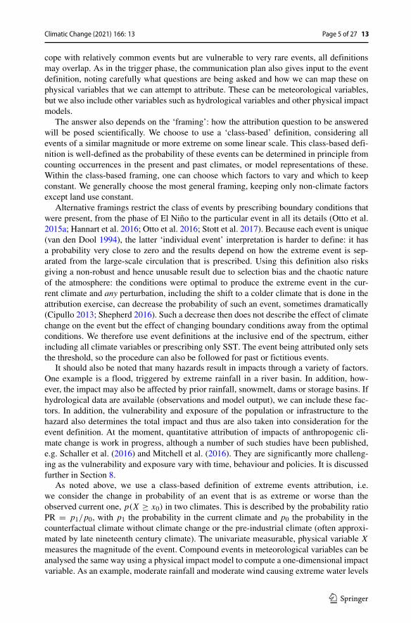
heat waves over India of CMIP5 models are incompatible with the observed trends due tomissing or misrepresented external forcings: an underestimation of aerosol cooling and theabsence of the effects of increased irrigation in these models (van Oldenborgh et al. 2018).The power of these tests depends strongly on the quality and quantity of the observations.Bad quality observations can cause a good model to be rejected and natural variability inthe observations can hide structural problems in a model.

Finally, ideally, we would like to check whether the extremes are caused by the samemeteorological mechanisms as in reality. This can involve checking a large number of pro-cesses, making it difficult in practice. However, investigations increase confidence in themodel’s ability to simulate extremes for the right reasons. King et al. (2016) demandedthat ENSO teleconnections to Indonesia were reasonable. More generally, Ciavarella et al.(2018) verify all SST influences. For the US Gulf Coast, van der Wiel et al. (2017) showedthat in both observations and models, about two-thirds of extreme precipitation events weredue to landfalling tropical storms and hurricanes and one-third due to other phenomena,such as the cut-off low that caused flooding in Louisiana in 2016. There have also beenattempts to trace back the water in extreme precipitation events (Trenberth et al. 2015; Edenet al. 2016), but these often found that the diversity of sources was too large to constrainmodels (Eden et al. 2018).

Quantitative meteorological checks are still under development (Vautard et al. 2018). Itis therefore still possible that the climate models we use generate the right extreme statisticsfor the wrong reasons.

The result of the model evaluation is a set of models that seem to represent the extremeevent under study well enough. We discard the others and proceed with this set, assumingthey all represent the real climate equally well. If there are no models that represent theextreme well enough, as in the case of the 2017 Sri Lanka floods, we either abandon theattribution study or publish only the observational results as a ‘quick-look’ analysis.

6 Modelled trends and differences with counterfactual climates

We now come to the extreme event attribution step originally proposed by Allen (2003):using climate models to compute the change in probability of the extreme event due tohuman influence on climate. There are two ways to do this. The most straightforward one,proposed by Allen (2003), is to run the climate model twice, once with the current climateand once with an estimate of what the climate would have been like without anthropogenicemissions, the counterfactual climate. With a large enough ensemble, we can just count theoccurrences above a threshold corresponding to the event of interest to obtain the probabil-ities. Alternatively, we estimate the probabilities with a fit to an extreme value function. Toaccount for model biases, we set the threshold at the same return time in the current climateas was estimated from the observed data rather than the same event magnitude. Bias cor-recting the position parameter was found to be problematic, as the event can end up abovethe upper limit that exists for some variables (notably heat).

The second way is to use transient climate experiments, such as the historical/RCP4.5experiments for CMIP5, and analyse these the same way as the observations. This assumesthat the major cause of the trends from the late nineteenth century until now in the modelsis due to anthropogenic emissions of greenhouse gases and aerosols, neglecting naturalforcings: solar variability and volcanic eruptions. Volcanic eruptions have short impacts onthe weather and therefore do not contribute much to long-term trends; the effects of changes

Climatic Change (2021) 166: 13Page 14 of 2713

in solar activity on the weather are negligible for most of the world in recent history (Pittock2009).

Simulations starting at the end of the nineteenth century are not available in the caseof regional climate simulations downscaling the CMIP simulations. Regional simulationsusually start in 1950 or 1970. As this includes most of the anthropogenic heating, we canextrapolate the trend to a starting date of 1900. The interpretation is complicated by manyregional simulations not including aerosol and land use changes.

For each of these two methods, there are different framings possible. We use two fram-ings: models in which the sea surface temperature (SST) either is prescribed or is internallygenerated by a coupled ocean model. This makes a difference when the local weatheris influenced by SSTs, for instance through an ENSO teleconnection. An example is theTexas drought and heat of 2011, where the drying due to La Nina exacerbated the temper-ature response to the anomalous circulation (Hoerling et al. 2013a). There are also regionswhere prescribing SST gives wrong teleconnection trends (e.g. Copsey et al., 2006), inother regions they have a more realistic climatology than coupled models. However, we findthat often differences between these two framings are smaller than the noise due to naturalvariability and systematic differences between different climate models. As mentioned inSection 3, other framings in which more of the boundary conditions are fixed are also in use.

This step gives for every model experiment studied an estimate for the probabilityratio (PR) and for the change in intensity I due to anthropogenic global warming, plusuncertainty estimates due to limited sampling of the natural variability. These uncertaintyestimates do not include the uncertainties due to model formulations and framing. Thespread across multiple models and framings gives an indication of these and is used in thenext step.

7 Hazard synthesis

Next, we combine all the information generated from the observations and different well-evaluated models into a single attribution statement for the physical extreme, the hazardin risk analysis terminology. This step follows from the inclusion of observational trendsand from the experience that a multi-model ensemble is much more reliable than a singlemodel (Hagedorn et al. 2005). The best way to do this is still an area of active research.Our procedure is first to plot the probability ratios and changes in intensity including uncer-tainties due to natural variability. This shows whether the model results are compatiblewith the estimates from observations and whether they are compatible with each other.As model experiments may have multiple ensemble members or long integrations, and theobservations are based on a single earth and relatively short time series, the statisticaluncertainties due to natural variability are generally smaller in the model results. The largeuncertainties in the observed trend reflect the fact that changes in many extremes are onlyjust emerging over the noise of natural variability. This explains some apparent discrepan-cies between models and observations, for instance the ‘East Africa paradox’ that modelssimulate a wetting trend whereas the observations show drying: even without taking decadalvariability into account the uncertainties around the observed trend easily encompass themodelled trends (Uhe et al. 2018; Philip et al. 2018b).

If all model results are compatible with each other and with the observations (as shownby χ2/dof ≈ 1), the spread is mainly due to natural variability and a simple (weighted)mean can be taken over all results to give the final attribution result. An example is shownin Fig. 5a. Another possibility is that the models disagree, as in Fig. 5b: one model shows

Climatic Change (2021) 166: 13 Page 15 of 27 13

an 8% increase compatible with Clausius-Clapeyron scaling, but another model has a twotimes larger increase (the third model did not pass the model evaluation step). In thiscase, model spread is important and the uncertainty on the attribution statement shouldreflect this.

These synthesis plots can also be used to illustrate that essential processes are missingor misrepresented in the models, as in Fig. 5c, showing the probability ratios for a windstorm like Friederike on 18 January 2018. It is clear that the observed strong negative trendis incompatible with the modelled weak positive trends (Vautard et al. 2019), so we cannotprovide an attribution statement.

If possible, the synthesis can also include an outlook to the future, based on extrapolationof trends to the near future or model results. This is frequently requested by users of theattribution results.

0.1 1 10

OBS

HadGEM3A

weather@home

RACMO

CORDEX

Weighted average

-20 -10 0 10 20 30

localregional

(a) Intensity change (%)

GHCN-D 30yr stationsGHCN-D 80yr stations

CPC 0.5 analysis

GHCN-D 80yr stationsCPC 0.5 analysis

EC-Earth T799GFDL HiFLOR

Average

0.00001 0.0001 0.001 0.01 0.1 1

ISD-lite

RACMO

EURO-CORDEX

b

a

c

Fig. 5 Synthesis plots of a the probability ratio of extreme 3-day averaged precipitation in April–June aver-aged over the Seine basin (Philip et al. 2018a), b the intensity of extreme 3-day precipitation on the GulfCoast (van Oldenborgh et al. 2017) and c the probability ratio for changes in wind intensity over the regionof storm Friederike on 18 January 2018 Vautard et al. (2019). Observations are shown in blue, models in redand the average in purple

Climatic Change (2021) 166: 13Page 16 of 2713

8 Vulnerability and exposure analysis

It is well documented in disasters literature that the impacts of any hazard, in this casehydrometeorological hazards, are due to a combination of three factors (United Nations2009):

1. the hydrometeorological hazard: process or phenomenon of atmospheric, hydrologicalor oceanographic nature that may cause loss of life, injury or other health impacts,property damage, loss of livelihoods and services, social and economic disruption, orenvironmental damage,

2. the exposure: people, property, systems or other elements present in hazard zones thatare thereby subject to potential losses, and

3. the vulnerability: the characteristics and circumstances of a community, system or assetthat make it susceptible to the damaging effects of a hazard.

The interplay of these three components determines whether or not a disaster results (Fieldet al. 2012). As we usually choose to base the event trigger and definition on severe societalimpacts of a natural hazard, rather than the purely physical nature of the extreme event, itis critical to also analyse trends in vulnerability and exposure in order to put the attributionresults in context. Our analyses therefore include drivers that have changed exposure as wellas vulnerability (which includes the capacity to manage the risk).

Due to the complexity of assessing changes in vulnerability and exposure as well asthe persistent lack of standardised, granular (local or aggregated) data (Field et al. 2012),usually only a qualitative approach is feasible (cf. Cramer et al., 2014). This includes (1) areview and categorisation of the people, assets and systems that affected or were affectedby the physical hazard extreme (done partly already in the event definition stage), (2) areview of existing peer-reviewed and select grey literature that describes changes to thevulnerability or exposure of the key categories of people, assets or systems over the pastfew decades and (3) key informant interviews with local experts. These results are thensynthesised into an overview of key factors which may have enhanced or diminished theimpacts of the extreme natural hazard. As the methodology associated with this analysis hasadvanced, the integration of this information into attribution studies has progressed from anintroductory framing to incorporating findings in synthesis or conclusions sections to mostrecently including a stand-alone vulnerability and exposure section (Otto et al. 2015b; vanOldenborgh et al. 2017; Otto et al. 2018a; van Oldenborgh et al. 2020).

Analysis of vulnerability and exposure can significantly impact the overall narrativeresulting from an attribution study as well as subsequent real-world actions which mayresult. For example an attribution study of the 2014–2015 drought in Sao Paulo, Brazil (Ottoet al. 2015b) found that, contrary to widespread belief, anthropogenic climate change wasnot a major driver of the water scarcity in the city. Instead, the analysis showed that theincrease of population of the city by roughly 20% in 20 years, and the even faster increasein per capita water usage, had not been addressed by commensurate updates in the storageand supply systems. Hence, in this case, the trends in vulnerability and exposure were themain driver of the significant water shortages in the city.

Similarly, a study of the 2015 drought in Ethiopia also found that while the drought wasextremely rare, occurring with a lower bound estimate of once every 60 years, there was nodetectable climate change influence. However in contrast to the Sao Paulo example, Ethiopiaoverall has seen drastic reduction in its population’s vulnerability, with the number of peopleliving in extreme poverty dropping by 22 percentage points between 2000 and 2011 (World

Climatic Change (2021) 166: 13 Page 17 of 27 13

Bank 2018). This indicates that although roughly 1.7 million people were impacted in 2015with moderate to acute malnutrition, the worst effects of the drought may have been avoided(Philip et al. 2018b). Just like trends in the hazard, trends in vulnerability and exposure cango both ways.

Vulnerability and exposure trends also play an important role in contextualising attribu-tion results when a climate change influence is detected. For example, the 2016 study offlooding in France underscores the complexity and double jeopardy faced by water systemmanagers in a changed climate, even when vulnerability and exposure trends are broadlymanaged well. In this case, a multi-reservoir system exists to reduce flood and drought risksthroughout the year and reservoir managers follow daily retention targets to manage thesystem. In anticipation of entering the dry season, where reservoirs are needed to regulateshipping and drinking water to 20 million people, the system was 90% full and unable toabsorb excess river runoff. In addition to the extreme rainfall and its increased likelihooddue to climate change, the late occurrence of the event and the reservoir regime also playedan important role in the sequence of events (Philip et al. 2018a).

The attribution study of the 2003 European heatwaves, combined with other studies onvulnerability and exposure during the same event, underscores the deadly impact of the com-bination of climate trends with an unprepared, vulnerable population, emphasising the needto establish early warning systems and adapt public health systems to prepare for increasedrisks (Stott et al. 2004; Kovats and Kristie 2006; Fouillet et al. 2008; de’ Donato et al.2015). Similarly, the 2017 study of Hurricane Harvey underscores how rising risk emergesfrom a significant trend in extreme rainfall combined with vulnerability and exposure fac-tors such as ageing infrastructure, urban growth policies and high population pressure (vanOldenborgh et al. 2017; Sebastian et al. 2019).

Despite the importance of the vulnerability and exposure analysis in ensuring a com-prehensive overview of attribution results, we have encountered a few challenges inincorporating it into attribution studies. Firstly, it is usually at least partly qualitative andthus requires extensive consultation to ensure that the final summary is comprehensive,accurate and not biased by preconceptions or political agendas. There is a lack of stan-dardised indicators that can be used to create a common, quantitative metric across studies.Finally, within attribution studies, vulnerability and exposure sections are often viewed asexcess information, making it a prime location to reduce paper lengths in order to meetjournal restrictions. This in turn limits the contributions and advancements in this area ofanalysis.

9 Communication

As mentioned in the introduction, we consider three groups of users of the results of ourstudies: people who ask the question, the adaptation community and participants in themitigation debate. Tailored communication of the results of an attribution study is an impor-tant final step in ensuring the maximum uptake of the study’s findings. WWA from thebeginning has contained communication experts and social scientists as recommended by,e.g. Fischoff (2007). We found that the key audiences that are interested in our attributionresults should be stratified according to their level of expertise: scientists, policy-makersand emergency management agencies, media outlets and the general public. Over theyears, we developed methods to present the results in tailored outputs intended for thoseaudiences.

Climatic Change (2021) 166: 13Page 18 of 2713

In presenting results to the scientific community, a focus on allowing full reproducibilityis key. We always publish a scientific report that documents the attribution study in sufficientdetail for another scientist to be able to reproduce or replicate the study’s results. If thereare novel elements to the analysis, the paper should also undergo peer review. We havefound that this documentation is also essential to ensure consistency within the team onnumbers and conclusions. We recommend that all datasets used are also made publiclyavailable (if not prohibited by the restrictive data policies of some national meteorologicalservices).

We have found it very useful to summarise the main findings and graphs of the attributionstudy into a two-page scientific summary aimed at science-literate audiences who prefer asnapshot of the results. Such audiences include communication experts associated with thestudy, science journalists and other scientists seeking a brief summary.

For policy-makers, humanitarian aid workers and other non-scientific professional audi-ences, we found that the most effective way to communicate attribution findings in writtenform are briefing notes that summarise the most salient points from the physical scienceanalysis (the event definition; past, present and possibly future return period; role of climatechange), elaborate on the vulnerability and exposure context and then provide specific rec-ommended next steps to increase resilience to this type of extreme event (Singh et al. 2019).These briefing notes can also be accompanied by a bilateral or roundtable dialogue processbetween these audiences and study experts in order to expound on any questions that mayarise. The in-person follow-up is often critical to help non-experts interpret and apply thescientific findings to their contexts. For example, return periods, which are the standard forpresenting probabilities of an extreme event to scientists and engineers, are often misun-derstood and require further explanation and visualisation. This audience often requires theinformation to be available relatively quickly after the event (Holliday 2007; de Jong et al.2019).

In order to reach the general public via the media, a press release and/or website newsitem can be prepared that communicates, in simplified language, the primary findings of thestudy. In addition to the physical science findings, these press releases typically provide avery brief, objective description of the non-physical science factors that contributed to theevent. In developing this press piece, study authors need to be as unbiased as possible, forinstance not emphasising lower bounds as conservative results (Lewandowsky et al. 2015).Consideration for how a press release will be translated into the press is also important. Welearned to avoid the phrase ‘at least’ to indicate a lower boundary of a confidence interval,as it is almost always dropped after which the lower boundary is reported as the most likelyresult, as in the press release of Kew et al. (2019). Van der Bles et al. (2018) found that anumerical confidence interval (‘X (between Y and Z)’) does not decrease confidence in thefindings, but verbal uncertainty communication (e.g. the phrase ‘with a large uncertainty’)does, both relative to not mentioning the uncertainties. Ensuring that study authors, espe-cially local authors, are available for interviews can help to ensure that additional questionson study findings are clarified as accurately as possible.

It should also be noted that despite these general lessons learned on communicationto general media in Western countries, effective communication of attribution findings iscontext-specific. This was shown by research in the context of attribution studies by theWWA consortium in East Africa and South Asia (Budimir and Brown 2017). This study alsoprovides evidence-based advice, including basic phrases that are most likely to be under-stood for specific stakeholder groups, but also cautions about the context-specific natureof this advice, and the need to work with communications advisers and representatives ofstakeholder groups for specific contexts to ensure effective communication.

Climatic Change (2021) 166: 13 Page 19 of 27 13

When communicating with various audiences, we also found it useful to considerresearch on communication strategies for analogous types of climate messages. Padghamet al. (2013) specifically looked at vulnerable communities in developing countries andunderscored the importance of using locally relevant terms and the need for knowledge co-generation and social learning between researchers and communities. WWA partner, theRed Cross Red Crescent Climate Centre relies on the global Red Cross Red Crescent net-work of national societies in over 190 countries to quickly get local input on the extremeevent in question, including their input on any press releases that will go out sharing the find-ings of the studies. For example, in Kenya, when studying the impacts of 2016/17 drought,we sought inputs from the Kenya Red Cross on how best to share the findings of the attribu-tion research. For this particular context, it was important to provide the attribution results(which did not indicate anthropogenic climate change played a role in the lack of rainfall)in the context of the seasonal forecast for the upcoming rainy season so that decision mak-ers could compare and differentiate between the short-term rainfall variability and potentialrole of climate change.

Scienseed (2016) address issues relating to jargon, complexity and impersonality, as wellas the need to be aware of mental models and biases through which information may be filte-red. Martin et al. (2008) show lessons on communication of forecast uncertainty, also pointsto the need to understand users’ interpretations and invest in communication that is bothclear and consistent from a scientific perspective, and tuned to how it will be interpreted.

In recent years attribution, experts are also exploring less traditional ways of communi-cating attribution findings. This includes the use of a ‘serious game’ to simulate the processa climate model undergoes to produce the statistics used in extreme event attribution (Parkeret al. 2016). A modified version of this game has been used by WWA with stakeholders,including scientists, disaster managers and policymakers, in India and Ethiopia to explainthe findings of studies conducted in both these countries.

10 Conclusions

In this paper, we have summarised the lessons we learned in doing rapid and slow attribu-tion studies of extreme weather and climate events following guidance from the scientificliterature. We have developed an eight-step procedure that worked well in practice, basedon the following lessons we learned along the way.

1. We need a way to decide which extremes to investigate and which not, given finiteresources. In our case, human impacts were the main driver.

2. As many others, we found that the results can depend strongly on the event definition,which should be carefully defined. An WWA event definition aims to characterise thehazard in a way that best matches the most relevant impact of the event, yet also enableseffective scientific analysis.

3. A key step in our analysis is the analysis of changes in probability of this extreme inthe observed record. This also allows the estimation of the probability in the currentclimate, which is often requested. It also provides benchmarks for quantitative modelevaluation and trend estimates.

4. We need large ensembles or long experiments of multiple climate models and onlyuse the models that represent the extreme under study in agreement with the observedrecord.

Climatic Change (2021) 166: 13Page 20 of 2713

5. We need to pay attention that the key global and local forcings are taken into account inthe different models to give realistic total trends. Local factors such as aerosol forcings,land use changes and irrigation can be just as important as greenhouse gases. SST-forced models can give different results from coupled models.

6. A careful synthesis of the observational and model results is needed, keeping theuncertainties due to natural variability and model uncertainties separate.

7. Results of the physical hazard analysis should be paired with a description of the vulner-ability and exposure and trends in these factors, so trends in impacts are not attributedsolely to trends in the hazard, even in the case of a strong attribution to climate changeof the physical hazard.

8. We need to communicate in different ways to different audiences, but always shouldwrite up a full scientific text as a basis for communication, which also enablesreplicability and hence trust.

Taking these key points into account, we found that often, we could find a consistent mes-sage from the attribution study in the imperfect observations and model simulations. Thiswe used to inform key audiences with a solid scientific result, in many cases quite quicklyafter the event when the interest is often highest. However, we also found many cases wherethe quality of the available observations or models was just not good enough to be able tomake a statement on the influence of climate change on the event under study. This alsopoints to scientific questions on the reliability of projections for these events and the needfor model improvements.

Over the last 5 years, we found that when we can give answers, these are useful forinforming risk reduction for future extremes after an event, and in the case of strong resultsalso to raise awareness about the rising risks in a changing climate and thus the relevanceof reducing greenhouse gas emissions. Most importantly, the results are relevant simplybecause the question is often asked—and if it is not answered scientifically, it will beanswered unscientifically.

Author contribution All authors participated in the extreme event attribution studies on which this articleis based. GJvO provided the first draft, and all co-authors provided text for the final version.

Funding This paper builds on results from the Copernicus COP 039 and C3S 62 contracts lead by KNMI,which focused on the development of a prototype for extreme events and attribution service within the contextof the Copernicus Climate Change Service (C3S) implemented by the European Centre for Medium-RangeWeather Forecasts (ECMWF) and funded by the European Union. The Red Cross Red Crescent Climate Cen-tre authors were partly supported by the Partners for Resilience program. AK was funded by the AustralianResearch Council (DE180100638).

Data availability Most data is available for analysis and download via the KNMI Climate Explorer(climexp.knmi.nl) under ‘Attribution runs’. The exceptions are the NOAA radar data (Fig. 1c), which canbe downloaded from their servers, and the synthesis data of Fig. 5, which are available on request from theauthors.

Code availability The code of the KNMI Climate Explorer web application, which was used to produce allfigures, is publicly available on GitLab.

Climatic Change (2021) 166: 13 Page 21 of 27 13

Declarations

Conflict of interest The authors declare no competing interests.

Open Access This article is licensed under a Creative Commons Attribution 4.0 International License, whichpermits use, sharing, adaptation, distribution and reproduction in any medium or format, as long as you giveappropriate credit to the original author(s) and the source, provide a link to the Creative Commons licence,and indicate if changes were made. The images or other third party material in this article are included in thearticle’s Creative Commons licence, unless indicated otherwise in a credit line to the material. If material isnot included in the article’s Creative Commons licence and your intended use is not permitted by statutoryregulation or exceeds the permitted use, you will need to obtain permission directly from the copyright holder.To view a copy of this licence, visit http://creativecommons.org/licenses/by/4.0/.

References

Allen MR (2003) Liability for climate change. Nature 421(6926):891–892. https://doi.org/10.1038/421891aAngelil O, Stone DA, Tadross M, Tummon F, Wehner M, Knutti R (2014) Attribution of extreme weather

to anthropogenic greenhouse gas emissions: sensitivity to spatial and temporal scales. Geophys Res Lett41(6):2150–2155. https://doi.org/10.1002/2014GL059234

Angelil O, Perkins-Kirkpatrick S, Alexander LV, Stone D, Donat MG, Wehner M, ShiogamaH, Ciavarella A, Christidis N (2016) Comparing regional precipitation and temperatureextremes in climate model and reanalysis products. Weather Clim Extremes 13:35–43.https://doi.org/https://doi.org/10.1016/j.wace.2016.07.001

Angelil O, Stone DA, Perkins SE, Alexander LV, Wehner MF, Shiogama H, Wolke R, Ciavarella A, ChristidisN (2018) On the nonlinearity of spatial scales in extreme weather attribution statements. Clim Dyn50:2739. https://doi.org/10.1007/s00382-017-3768-9

Bindoff NL, Stott PA et al (2013) Detection and attribution of climate change: from global to regional. In:Stocker TF et al (eds) Climate change 2013: the physical science basis, vol 10. Cambridge UniversityPress, Cambridge, pp 867–952

Budimir M, Brown S (2017) Communicating extreme event attribution. Tech. rep., The Schumacher Cen-tre, Bourton on Dunsmore, Rugby, Warwickshire, UK.. www.climatecentre.org/downloads/files/FULL%20REPORT%20final.pdf

Cattiaux J, Ribes A (2018) Defining single extreme weather events in a climate perspective. Bull Amer MetSoc 99(8):1557–1568. https://doi.org/10.1175/BAMS-D-17-0281.1

Ciavarella A, Christidis N, Andrews M, Groenendijk M, Rostron J, Elkington M, Burke C, Lott FC,Stott PA (2018) Upgrade of the HadGEM3-A based attribution system to high resolution anda new validation framework for probabilistic event attribution. Weather Clim Extremes 20:9–32.https://doi.org/10.1016/j.wace.2018.03.003

Cipullo ML (2013) High resolution modeling studies of the changing risks or damage from extratropicalcyclones. North Carolina State University, PhD thesis

Copsey D, Sutton R, Knight JR (2006) Recent trends in sea level pressure in the Indian Ocean region.Geophys Res Lett 33(19). https://doi.org/10.1029/2006GL027175

Cramer W, Yohe GW, Auffhammer M, Huggel C, Molau U, da Silva Dias M, Solow A, Stone DA, TibigL (2014) Detection and attribution of observed impacts. In: Field CB et al (eds) Climate change 2014:impacts, adaptation, and vulnerability. part A: global and sectoral aspects, vol 18. Cambridge UniversityPress, Cambridge and New York, pp 979–1037

D’Ippoliti D, Michelozzi P, Marino C, de’Donato F, Menne B, Katsouyanni K, Kirchmayer U, AnalitisA, Medina-Ramon M, Paldy A, Atkinson R, Kovats S, Bisanti L, Schneider A, Lefranc A, IniguezC, Perucci CA (2010) The impact of heat waves on mortality in 9 European cities: results from theEuroHEAT project. Environ Health 9(1):37. https://doi.org/10.1186/1476-069X-9-37

de’ Donato FK, Leone M, Scortichini M, De Sario M, Katsouyanni K, Lanki T, Basagana X, Ballester F,Astrom C, Paldy A, Pascal M, Gasparrini A, Menne B, Michelozzi P (2015) Changes in the effect of heaton mortality in the last 20 years in nine European cities. results from the PHASE project. Int J EnvironRes Public Health 12(12):15567–15583. https://doi.org/10.3390/ijerph121215006

de Jong J, Hansen J, Groenewegen P (2019) Why do we need for timeliness of research in decision-making?Eur J Public Health 29(Supplement 4). https://doi.org/10.1093/eurpub/ckz185.216, ckz185.216

Climatic Change (2021) 166: 13Page 22 of 2713

de Vries H, van Westrhenen R, Oldenborgh van (2012) GJ (2013) The European cold spell that didn’t bringthe Dutch another 11-city tour. In: Peterson TC, Hoerling MP, Stott PA, Herring SC (eds) ExplainingExtreme Events of 2012 from a Climate Perspective, vol 94, Bull. Amer. Met. Soc., pp S26–S28

Easterling DR, Kunkel KE, WM F, Sun L (2016) Detection and attribution of climate extremes in theobserved record. Weather Clim Extremes 11:17–27. https://doi.org/10.1016/j.wace.2016.01.001

Eden JM, Wolter K, Otto FEL, van Oldenborgh GJ (2016) Multi-method attribution anal-ysis of extreme precipitation in Boulder, Colorado. Environ Res Lett 11(12):124009.https://doi.org/10.1088/1748-9326/11/12/124009

Eden JM, Kew SF, Bellprat O, Lenderink G, Manola I, Omrani H, van Oldenborgh GJ (2018) Extremeprecipitation in the Netherlands: an event attribution case study. Weather Clim Extremes 21:90–101.https://doi.org/10.1016/j.wace.2018.07.003

Efron B, Tibshirani RJ (1998) An introduction to the bootstrap. Chapman and Hall, New YorkField CB, Barros V, Stocker TF, Qin D, Dokken DJ, Ebi KL, Mastrandrea MD, Mach KJ, Plattner GK, Allen

SK, Tignor M, Midgley PM (eds) (2012) Managing the risks of extreme events and disasters to advanceclimate change adaptation. Cambridge University Press, Cambridge

Fischer EM, Beyerle U, Knutti R (2013) Robust spatially aggregated projections of climate extremes. NatClim Change 3:1033–1038. https://doi.org/10.1038/nclimate2051

Fischoff B (2007) Nonpersuasive communication about matters of greatest urgency: climate change. EnvironSci Technol 41(21):7204–7208. https://doi.org/10.1021/es0726411

Fouillet A, Rey G, Wagner V, Laaidi K, Empereur-Bissonnet P, Le Tertre A, Frayssinet P, Bessemoulin P,Laurent F, De Crouy-Chanel P, Jougla E, Hemon D (2008) Has the impact of heat waves on mortalitychanged in France since the european heat wave of summer 2003? a study of the 2006 heat wave. Int JEpidemiology 37(2):309–317. https://doi.org/10.1093/ije/dym253

Hagedorn R, Doblas-Reyes FJ, Palmer TN (2005) The rationale behind the success of multi-model ensembles in seasonal forecasting – I. Basic concept. Tellus A 57(3):219–233.https://doi.org/10.1111/j.1600-0870.2005.00103.x

Hanel M, Buishand TA, Ferro CAT (2009) A nonstationary index flood model for precipitationextremes in transient regional climate model simulations. J Geophys Res Atmos 114(D15):D15107.https://doi.org/10.1029/2009JD011712

Hannart A, Carrassi A, Bocquet M, Ghil M, Naveau P, Pulido M, Ruiz J, Tandeo P (2016) DADA:data assimilation for the detection and attribution of weather and climate-related events. Clim Change136(2):155–174. https://doi.org/10.1007/s10584-016-1595-3

Hauser M, Gudmundsson L, Orth R, Jezequel A, Haustein K, Vautard R, van Oldenborgh GJ, Wilcox L,Seneviratne SI (2017) Methods and model dependency of extreme event attribution: The 2015 Europeandrought. Earth’s Future 5(10):1034–1043. https://doi.org/10.1002/2017EF000612

Hoerling M, Kumar A, Dole R, Nielsen-Gammon JW, Eischeid J, Perlwitz J, Quan XW, ZhangT, Pegion P, Chen M (2013a) Anatomy of an extreme event. J Clim 26(9):2811–2832.https://doi.org/10.1175/JCLI-D-12-00270.1

Hoerling M, Eischeid J, Kumar A, Leung R, Mariotti A, Mo K, Schubert S, Seager R (2014)Causes and predictability of the 2012 great plains drought. Bull Amer Met Soc 95(2):269–282.https://doi.org/10.1175/BAMS-D-13-00055.1

Hoerling MP, Wolter K, Perlwitz J, Quan X, Escheid J, Wang H, Schubert S, Diaz HF, Dole RM(2013b) Northeast Colorado extreme rains interpreted in a climate change context. Bull Amer Met Soc95(9):S15–S18

Holliday L (ed) (2007) Agricultural water management. The National Academies Press, Washington.https://doi.org/10.17226/11880, p.30

Kendon EJ, Roberts NM, Fowler HJ, Roberts MJ, Chan SC, Senior CA (2014) Heavier summer down-pours with climate change revealed by weather forecast resolution model. Nat Clim Change 4:570–576.https://doi.org/10.1038/nclimate2258

Kew SF, Philip SY, van Oldenborgh GJ, Otto FE, Vautard R, van der Schrier G (2019) Theexceptional summer heatwave in southern Europe 2017. Bull Amer Met Soc 100(1):S2–S5.https://doi.org/10.1175/BAMS-D-18-0109.1

Kew SF, Philip SY, Hauser M, Hobbins M, Wanders N, van Oldenborgh GJ, van der Wiel K, Veldkamp TIE,Kimutai J, Funk C, Otto FEL (2021) Impact of precipitation and increasing temperatures on droughttrends in eastern Africa. Earth Syst Dyn 12(1):17–35. https://doi.org/10.5194/esd-12-17-2021

King AD, Alexander LV, Donat MG (2013) The efficacy of using gridded data to examineextreme rainfall characteristics: a case study for Australia. Int J Climatol 33(10):2376–2387.https://doi.org/10.1002/joc.3588

King AD, van Oldenborgh GJ, Karoly DJ (2016) Climate change and El Nino increase likelihood of Indone-sian heat and drought. Bull Amer Met Soc 97:S113–S117. https://doi.org/10.1175/BAMS-D-16-0164.1

Climatic Change (2021) 166: 13 Page 23 of 27 13

Kirchmeier-Young MC, Zwiers FW, Gillett NP, Cannon AJ (2017) Attributing extreme fire risk in WesternCanada to human emissions. Clim Change 144(2):365–379. https://doi.org/10.1007/s10584-017-2030-0

Kovats RS, Kristie LE (2006) Heatwaves and public health in Europe. Eur J Public Health 16(6):592–599.https://doi.org/10.1093/eurpub/ckl049

Krikken F, Lehner F, Haustein K, Drobyshev I, van Oldenborgh GJ (2019) Attribution of the role ofclimate change in the forest fires in Sweden 2018. Nat Hazards Earth Syst Sci Discuss 2019:1–24.https://doi.org/10.5194/nhess-2019-206

Leach NJ, Li S, Sparrow S, van Oldenborgh GJ, Lott FC, Weisheimer A, Allen MR (2020) Anthropogenicinfluence on the 2018 summer warm spell in Europe: the impact of different spatio-temporal scales. BullAmer Met Soc 101(1):S41–S46. https://doi.org/10.1175/BAMS-D-19-0201.1

Lenderink G, van Meijgaard E (2010) Linking increases in hourly precipitation extremesto atmospheric temperature and moisture changes. Environ Res Lett 5:025208,.https://doi.org/10.1088/1748-9326/5/2/025208, http://stacks.iop.org/1748-9326/5/i=2/a=025208

Lewandowsky S, Oreskes N, Risbey JS, Newell BR, Smithson M (2015) Seepage: Climate changedenial and its effect on the scientific community. Glob Environ Chang 33(Supplement C):1–13.https://doi.org/10.1016/j.gloenvcha.2015.02.013

Li C, Sun Y, Zwiers F, Wang D, Zhang X, Chen G, Wu H (2020) Rapid warming in summer wetbulb globe temperature in China with human-induced climate change. J Climate 33(13):5697–5711.https://doi.org/10.1175/JCLI-D-19-0492.1

Li Z, Chen Y, Fang G, Li Y (2017) Multivariate assessment and attribution of droughts in Central Asia. SciRep 7(1):1316. https://doi.org/10.1038/s41598-017-01473-1

Lobell DB, Bonfils C, Faures JM (2008) The role of irrigation expansion in past and future temperaturetrends. Earth Interactions 12(3):1–11. https://doi.org/10.1175/2007EI241.1

Luu LN, Vautard R, P Y vanOldenborghGJ, Lenderink G (2018) Attribution of extreme rainfallevents in the south of France using EURO-CORDEX simulations. Geophys Res Lett 45:6242–625.https://doi.org/10.1029/2018GL077807

Martin C, Cacic I, Mylne K, Rubiera J, Dehui C, Jiafeng G, Xu T, Yamaguchi M, Foamouhoue AK, PoolmanE, Guiney J, Kootval H (2008) Guidelines on communicating forecast uncertainty. WMO/TD 1422,WMO, Geneva, Switzerland. library.wmo.int/doc num.php?explnum id=4687

McGregor GR (2012) Special issue: Universal Thermal Comfort Index (UTCI). Int J Biometeorol 56(3):419–419. https://doi.org/10.1007/s00484-012-0546-6

Mitchell D, Heaviside C, Vardoulakis S, Huntingford C, Masato G, Guillod BP, Frumhoff P, Bowery A,Wallom A, Allen MR (2016) Attributing human mortality during extreme heat waves to anthropogenicclimate change. Environ Res Lett 11(7):074006. https://doi.org/10.1088/1748-9326/11/7/074006

Murakami H, Vecchi GA, Underwood S, Delworth TL, Wittenberg AT, Anderson WG, Chen JH, GudgelRG, Harris LW, Lin SJ, Zeng F (2015) Simulation and prediction of category 4 and 5 hurri-canes in the high-resolution GFDL HiFLOR coupled climate model. J Climate 28(23):9058–9079.https://doi.org/10.1175/JCLI-D-15-0216.1

Nag PK, Nag A, Sekhar P, Pandt S (2009) Vulnerability to heat stress: scenario in Western India.WHO APW SO 08 AMS 6157206, National Institute of Occupational Health, Ahmedabad.https://www.who.int/docs/default-source/searo/india/health-topic-pdf/occupational-health-vulnerability-to-heat-stress-scenario-of-western-india.pdf?sfvrsn=9568d2b6 2

National Academies of Sciences Engineering, and Medicine (2016) Attribution of extremeweather events in the context of climate change. The National Academies Press, Washington.https://doi.org/10.17226/21852

Otto F, Boyd E, Jones RG, Cornforth RJ, James R, Parker HR, Allen MR (2015a) Attribution of extremeweather events in Africa: a preliminary exploration of the science and policy implications. Clim Change132:531–543. https://doi.org/10.1007/s10584-015-1432-0

Otto FE (2017) Attribution of weather and climate events. Annu Rev Environ Resour 42(1):627–646.https://doi.org/10.1146/annurev-environ-102016-060847

Otto FEL, Coelho CAS, King A, Coughlan de Perez E, Wada Y, van Oldenborgh GJ, HaarsmaR, Haustein K, Uhe P, van Aalst M, Aravequia JA, Almeida W, Cullen H (2015b) Factorsother than climate change, main drivers of 2014/15 water shortage in southeast Brazil, vol 96.https://doi.org/10.1175/BAMS-D-15-00120.1

Otto FEL, van Oldenborgh GJ, Eden JM, Stott PA, Karoly DJ, Allen MR (2016) The attribution question.Nature Clim Change 6(9):813–816. https://doi.org/10.1038/nclimate3089

Otto FEL, van der Wiel K, van Oldenborgh GJ, Philip SY, Kew SF, Uhe P, Cullen H (2018a) Cli-mate change increases the probability of heavy rains in northern England/southern Scotland likethose of storm Desmond—a real-time event attribution revisited. Environ Res Lett 13(2):024006.https://doi.org/10.1088/1748-9326/aa9663

Climatic Change (2021) 166: 13Page 24 of 2713

Otto FEL, Wolski P, Lehner F, Tebaldi C, van Oldenborgh GJ, Hogesteeger S, Singh R, Holden P, FuckarNS, Odoulami R, New M (2018a) Anthropogenic influence on the drivers of the Western Cape drought2015–2017. Environ Res Lett 13:124010. https://doi.org/10.1088/1748-9326/aae9f9

Otto FEL, Harrington L, Schmitt K, Philip S, Kew S, van Oldenborgh GJ, Singh R, Kimutai J, WolskiP (2020) Challenges to understanding extreme weather changes in lower income countries. Bull AmMeteorol Soc 101(10):E1851–E1860. https://doi.org/10.1175/BAMS-D-19-0317.1

Padgham J, Devisscher T, Chuluun T, Mtilatila L, Kaimila E, Mansingh I, Agyemang-Yeboah F, Oben F(2013) Building shared understanding and capacity for action: Insights on climate risk communicationfrom India, Ghana, Malawi, and Mongolia. Int J Communication 7:970–983

Pall P, Aina T, Stone DA, Stott PA, Nozawa T, Hilberts AGJ, Lohmann D, Allen MR (2011) Anthropogenicgreenhouse gas contribution to flood risk in England and Wales in autumn 2000. Nature 470(7334):382–385. https://doi.org/10.1038/nature09762

Parker HR, Cornforth RJ, Suarez P, Allen MR, Boyd E, James R, Jones RG, Otto FEL, Walton P (2016)Using a game to engage stakeholders in extreme event attribution science. Int J Disaster Risk Science7(4):353–365. https://doi.org/10.1007/s13753-016-0105-6

Perkins SE, Alexander LV, Nairn JR (2012) Increasing frequency, intensity and duration of observed globalheatwaves and warm spells. Geophys Res Lett 39(20). https://doi.org/10.1029/2012GL053361

Philip S, Sparrow S, Kew SF, van der Wiel K, Wanders N, Singh R, Hassan A, Mohammed K, Javid H,Haustein K, Otto FEL, Hirpa F, Rimi RH, Islam AS, Wallom DCH, van Oldenborgh GJ (2019) Attribut-ing the 2017 Bangladesh floods from meteorological and hydrological perspectives. Hydrol Earth SystSci 23:1409–1429. https://doi.org/10.5194/hess-23-1409-2019

Philip SY, Kew SF, van Oldenborgh GJ, Aalbers E, Otto FEL, Haustein K, Habets F, Singh R (2018a)Validation of a rapid attribution of the May/June 2016 flood-inducing precipitation in France to climatechange. J Hydrometeorol 19(11):1881–1898. https://doi.org/10.1175/JHM-D-18-0074.1

Philip SY, Kew SF, van Oldenborgh GJ, Otto FEL, O’Keefe S, Haustein K, King AD, Zegeye A, Eshetu Z,Hailemariam K, Singh RK, Jjemba E, Funk C, Cullen H (2018b) Attribution analysis of the Ethiopiandrought of 2015. J Climate 31(6):2465–2486. https://doi.org/10.1175/JCLI-D-17-0274.1

Philip SY, Kew SF, van Oldenborgh GJ, Otto FEL, Vautard R, van der Wiel K, King AD, Lott FC, ArrighiJ, Singh RP, van Aalst MK (2020a) A protocol for probabilistic extreme event attribution analyses. AdvStat Climatol Meteorol Oceanogr 6:177–203. https://doi.org/10.5194/ascmo-6-177-2020

Philip SY, Kew SF, van der Wiel K, Wanders N, van Oldenborgh GJ (2020b) Regional differentia-tion in climate change induced drought trends in the Netherlands. Environ Res Lett 15:094081.https://doi.org/10.1088/1748-9326/ab97ca

Pittock AB (2009) Can solar variations explain variations in the earth’s climate? Clim Change 96(4):483–487.https://doi.org/10.1007/s10584-009-9645-8

Puma MJ, Cook BI (2010) Effects of irrigation on global climate during the 20th century. J Geophys ResAtmos 115(D16):D16120. https://doi.org/10.1029/2010JD014122, d16120

Rupp DE, Mote PW, Bindoff NL, Stott PA, Robinson DA (2013) Detection and attribution ofobserved changes in northern hemisphere spring snow cover. J Climate 26(18):6904–6914.https://doi.org/10.1175/JCLI-D-12-00563.1

Schaller N, Kay AL, Lamb R, Massey NR, van Oldenborgh GJ, Otto FEL, Sparrow SN, Vautard R, Yiou P,Bowery A, Crooks SM, Huntingford C, Ingram WJ, Jones RG, Legg T, Miller J, Skeggs J, Wallom D,Weisheimer A, Wilson S, Allen MR (2016) The human influence on climate in the winter 2013/2014floods in southern England. Nat Clim Change 6:627–634. https://doi.org/10.1038/nclimate2927

Scienseed SL (2016) Communicating climate change and biodiversity to policy makers. Tech. rep., Coun-cil of Europe, F-67075 Strasbourg Cedex. https://rm.coe.int/CoERMPublicCommonSearchServices/DisplayDCTMContent?\discretionarydocumentId=09000016806c11bb

Sebastian A, Gori A, Blessing RB, van der Wiel K, Bass B (2019) Disentangling the impacts of human andenvironmental change on catchment response during Hurricane Harvey. Environmental Research Letters14(12):124023. https://doi.org/10.1088/1748-9326/ab5234

Shepherd TG (2016) A common framework for approaches to extreme event attribution. Curr Clim ChangeRep 2(1):28–38. https://doi.org/10.1007/s40641-016-0033-y

Singh RK, Arrighi J, Coughlan de Perez E, Warrick O, Suarez P, Koelle B, Jjemba E, van Aalst MK,Roberts DC, Portner HO, Jones RG (2019) International conference on climate risk management, inputsfor the intergovernmental panel on climate change’s sixth assessment report. Clim Dev 11(8):655–658.https://doi.org/10.1080/17565529.2018.1521331

Sippel S, Walton P, Otto FEL (2015) Stakeholder perspectives on the attribution of extreme weather events:an explorative enquiry. Weather Clim Soc 7(3):224–237. https://doi.org/10.1175/WCAS-D-14-00045.1

Stott PA, Stone DA, Allen MR (2004) Human contribution to the European heatwave of 2003. Nature432(7017):610–614. https://doi.org/10.1038/nature03089

Climatic Change (2021) 166: 13 Page 25 of 27 13

Stott PA, Allen M, Christidis N, Dole RM, Hoerling M, Huntingford C, Pall P, Perlwitz J, Stone D (2013)Attribution of weather and climate-related events. In: Asrar GR, Hurrell JW (eds) Climate sciencefor serving society: research, modeling and prediction priorities. Springer, Dordrecht, pp 307–337.https://doi.org/10.1007/978-94-007-6692-1 12

Stott PA, Christidis N, Otto FEL, Sun Y, Vanderlinden JP, van Oldenborgh GJ, Vautard R, von Storch H,Walton P, Yiou P, Zwiers FW (2016) Attribution of extreme weather and climate-related events. WIREsClim Change 7:23–41. https://doi.org/10.1002/wcc.380

Stott PA, Karoly DJ, Zwiers FW (2017) Is the choice of statistical paradigm critical in extreme eventattribution studies? Clim Change 144:143–150. https://doi.org/10.1007/s10584-017-2049-2

Trenberth KE, Fasullo JT, Shepherd TG (2015) Attribution of climate extreme events. Nature Clim Change5(8):725–730. https://doi.org/10.1038/nclimate2657

Uhe P, Otto FEL, Haustein K, van Oldenborgh GJ, King A, Wallom D, Allen MR, Cullen H (2016) Compar-ison of methods: attributing the 2014 record European temperatures to human influences. Geophys ResLett 43:8685–8693. https://doi.org/10.1002/2016GL069568

Uhe P, Philip SY, Kew SF, Shah K, Kimutai J, Mwangi E, van Oldenborgh GJ, Singh RK, Arrighi J,Jjemba E, Cullen H, Otto FEL (2018) Attributing drivers of the 2016 Kenyan drought. Int J Climatol38(S1):e554–e568. https://doi.org/10.1002/joc.5389

United Nations (2009) 2009 UNISDR terminology on disaster risk reduction published by the United Nationsinternational strategy for disaster reduction (UNISDR), Geneva, Switzerland

van den Dool HM (1994) Searching for analogues, how long must one wait? Tellus 46A:314–324.https://doi.org/10.1034/j.1600-0870.1994.t01-2-00006.x

van den Hurk BJJM, van Meijgaard E, de Valk P, van Heeringen KJ, Gooijer J (2015) Analysis ofa compounding surge and precipitation event in the netherlands. Environ Res Lett 10(3):035001.https://doi.org/10.1088/1748-9326/10/3/035001

van der Bles AM, van der Linden S, Freeman A, Spiegelhalter D (2018) The effects of communicatinguncertainty about facts and numbers. In: Evidence-based medicine, BMJ, vol 23, pp A9–A10. https://ebm.bmj.com/content/23/Suppl 1/A9.2

van der Wiel K, Kapnick SB, Vecchi GA, Cooke WF, Delworth TL, Jia L, Murakami H, Underwood S,Zeng F (2016) The resolution dependence of contiguous U.S. precipitation extremes in response to CO2forcing. J Climate 29(22):7991–8012. https://doi.org/10.1175/JCLI-D-16-0307.1

van der Wiel K, Kapnick SB, van Oldenborgh GJ, Whan K, Philip SY, Vecchi GA, SinghRK, Arrighi J, Cullen H (2017) Rapid attribution of the August 2016 flood-inducing extremeprecipitation in south Louisiana to climate change. Hydrol Earth Syst Sci 21(2):897–921.https://doi.org/10.5194/hess-21-897-2017

van Oldenborgh GJ (2007) How unusual was autumn 2006 in Europe? Clim Past 3(4):659–668.https://doi.org/10.5194/cp-3-659-2007

van Oldenborgh GJ, de Vries H (2018) Code rood voor sneeuwval op 11 december 2017. Meteorologica27(1):24–25. climexp.knmi.nl/publications/Klimaatoverzicht maart2018.pdf, (in Dutch)

van Oldenborgh GJ, Otto FEL, Haustein K, Achuta Rao K (2016) The heavy precipita-tion event of December 2015 in Chennai, India. Bull Amer Met Soc 97(12):S87–S91.https://doi.org/10.1175/BAMS-D-16-0129.1

van Oldenborgh GJ, van der Wiel K, Sebastian A, Singh RK, Arrighi J, Otto FEL, Haustein K, Li S, VecchiGA, Cullen H (2017) Attribution of extreme rainfall from Hurricane Harvey, August 2017. Environ ResLett 12(12):124009. https://doi.org/10.1088/1748-9326/aa9ef2

van Oldenborgh GJ, Philip SY, Kew SF, van Weele M, Uhe P, Otto FEL, Singh RK, Pai I, Cullen H,AchutaRao K (2018) Extreme heat in India and anthropogenic climate change. Nat Hazards Earth SystSci 18(1):365–381. https://doi.org/10.5194/nhess-18-365-2018

van Oldenborgh GJ, Mitchell-Larson E, Vecchi G, de Vries H, Vautard R, Otto FE (2019)Cold waves are getting milder in the northern midlatitudes. Environ Res Lett 114004:14.https://doi.org/10.1088/1748-9326/ab4867

van Oldenborgh GJ, Krikken F, Lewis S, Leach NJ, Lehner F, Saunders KR, van Weele M, Haustein K, LiS, Wallom D, Sparrow S, Arrighi J, Singh RP, van Aalst MK, Philip SY, Vautard R, Otto FEL (2020)Attribution of the Australian bushfire risk to anthropogenic climate change. Natural. Nat Hazards andEarth Syst Sci. 941–960. https://doi.org/10.5194/nhess-21-941-2021

Vautard R, van Oldenborgh GJ, Thao S, Dubuisson B, Lenderink G, Ribes A, Soubeyroux JM, Yiou P,Planton S (2015) Extreme fall 2014 precipitations in the Cevennes mountain range. Bull Amer MeteorSoc 96(12):S56–S60. https://doi.org/10.1175/BAMS-D-15-00088.1

Vautard R, Christidis N, Ciavarella A, Alvarex-Castro C, Bellprat O, Christensen OB, Colfescu I, Cowan T,Doblas Reyes FJ, Eden JM, Hauser M, Hegerl GC, Hempelmann N, Klehmet K, Lott FC, Nangini C,Orth R, Radanovics S, Seneviratne SI, van Oldenborgh GJ, Stott PA, Tett S, Wilcox L, Yiou P (2018)

Climatic Change (2021) 166: 13Page 26 of 2713

Evaluation of the HadGEM3-A simulations in view of climate and weather event human influenceattribution in Europe. Clim Dyn 52:1187–1210. https://doi.org/10.1007/s00382-018-4183-6

Vautard R, van Oldenborgh GJ, Otto FEL, Yiou P, de Vries H, van Meijgaard E, Stepek A, Soubey-roux JM, Philip S, Kew SF, Costella C, Singh R, Tebaldi C (2019) Human influence on Euro-pean winter wind storms such as those of January 2018. Earth System Dynamics 10:271–286.https://doi.org/10.5194/esd-10-271-2019

Vautard R, van Aalst MK, Boucher O, Drouin A, Haustein K, Kreienkamp F, van Oldenborgh GJ, Otto FEL,Ribes A, Robin Y, Schneider M, Soubeyroux JM, Stott PA, Seneviratne SI, Vogel MM, Wehner MF(2020) Human contribution to the record-breaking June and July 2019 heat waves in Western Europe.Environ Res Lett 094077:15. https://doi.org/10.1088/1748-9326/aba3d4

Visser H, Petersen A (2009) The likelihood of holding outdoor skating marathons in theNetherlands as a policy-relevant indicator of climate change. Clim Change 93:39–54.https://doi.org/10.1007/s10584-008-9498-6

Wallace JM (2012) Weather- and climate-related extreme events: teachable moments. Eos Trans Am GeophysUnion 93(11):120–120. https://doi.org/10.1029/2012EO110004

Westra S, Alexander LV, Zwiers FW (2013) Global increasing trends in annual maximum daily precipitation.J Climate 26(11):3904–3918. https://doi.org/10.1175/JCLI-D-12-00502.1

Williams AP, Seager R, Abatzoglou JT, Cook BI, Smerdon JE, Cook ER (2015) Contribution of anthro-pogenic warming to California drought during 2012–2014. Geophys Res Lett 42(16):6819–6828.https://doi.org/10.1002/2015GL064924

World Bank (2018) The world bank in Ethiopia. http://www.worldbank.org/en/country/ethiopia/overview

Publisher’s note Springer Nature remains neutral with regard to jurisdictional claims in published mapsand institutional affiliations.

Climatic Change (2021) 166: 13 Page 27 of 27 13