Path relinking for high dimensional continuous optimization

Francisco Gortázar, Abraham Duarte

Dpto. de Ciencias de la ComputaciónDpto. de Ciencias de la Computación

Rafael Martí

Dpto. de Estadística e Investigación Operativa

� IntroductionIntroductionIntroductionIntroduction

� Path Relinking

Experimental results� Experimental results

� Conclusions

2

� Global optimization problems◦ Non linear function f(x)

◦ x={x1,…, xn}, l≤xi≤u◦ x={x1,…, xn}, l≤xi≤u

3

ℜ∈≤≤

x

uxl

xfMinimize )(

� Measuring success…◦ Scalability of Evolutionary Algorithms and other

Metaheuristics for Large Scale Continuous Optimization Problems, M. Lozano and F. Herrera Optimization Problems, M. Lozano and F. Herrera (Eds.), http://sci2s.ugr.es/eamhco/CFP.php

◦ 19 continuous functions

◦ Number of variables D={50,100,200,500,1000}

◦ Maximum number of evaluations: 5000D

� The search space is continuous…◦ Key issue: for which points will f(x) be evaluated?

4

� Introduction

� PathPathPathPath RelinkingRelinkingRelinkingRelinking


� Conclusions

5

Generate solutions

Selectsolutions bothby quality and

diversity (EliteSet)

Perform a path relinkingbetween each

pair of solutions

1 2 3

GRASP with PR for the MMDP 6

Return the best solution found so far4

� Path Relinking for Global Optimization (PR)◦ EliteSet construction (x1,...,xb)

◦ Improve x1, and replace it with the improved solutionsolution

◦ NewSubsets = (x,y), pair set of EliteSet solutions

◦ While NewSubsets ≠ ∅

� Select next pair (x,y) from NewSubsets

� Remove (x,y) from NewSubsets

� Perform a path relinking with (x,y) →w

� Improve w

� If f(w) < f(x1) then x1 = w

7

� EliteSet construction◦ Generate diverse solutions

� Sampling the solution space

◦ Based on ideas from factorial design of ◦ Based on ideas from factorial design of experiments

� Factorial design kn

� n, #variables

� k, #values

� Genichi Taguchi

8

� EliteSet construction◦ Factorial design example for

n=4, k=3

� 81 experiments

ExpExpExpExp.... FactoresFactoresFactoresFactores

1111 2222 3333 4444

1 1 1 1 1

2 1 2 2 2� 81 experiments

◦ Fractional design

� Taguchi Table L9(34)

� 9 experiments

9

2 1 2 2 2

3 1 3 3 3

4 2 1 2 3

5 2 2 3 1

6 2 3 1 2

7 3 1 2 3

8 3 2 1 3

9 3 3 2 1

� EliteSet construction◦ Taguchi method is applied to obtain diverse

solutions

◦ #values k = 3◦ #values k = 3

� midvalue = l + ½(u-l)

� lowervalue = l + ¼(u-l)

� uppervalue = l + ¾(u-l)

◦ #variables n∈{50,100,200,500,1000}

10

� EliteSet construction◦ Problem: biggest Taguchi table found: n=40

11

� EliteSet construction

x1x1x1x1 x2x2x2x2 x3x3x3x3 x4x4x4x4 x5x5x5x5 x6x6x6x6 x7x7x7x7 x8x8x8x8 X9X9X9X9

1 1 1 1 1 1 1 1 1

1 2 2 2 1 1 1 1 1

12

1 2 2 2 1 1 1 1 1

1 3 3 3 1 1 1 1 1

2 1 2 3 1 1 1 1 1

2 2 3 1 1 1 1 1 1

2 3 1 2 1 1 1 1 1

3 1 2 3 1 1 1 1 1

3 2 1 3 1 1 1 1 1

3 3 2 1 1 1 1 1 1



1 1 1 1 2 2 2 2 2

1 2 2 2 2 2 2 2 2

13

1 2 2 2 2 2 2 2 2

1 3 3 3 2 2 2 2 2

2 1 2 3 2 2 2 2 2

2 2 3 1 2 2 2 2 2

2 3 1 2 2 2 2 2 2

3 1 2 3 2 2 2 2 2

3 2 1 3 2 2 2 2 2

3 3 2 1 2 2 2 2 2



1 1 1 1 3 3 3 3 3

1 2 2 2 3 3 3 3 3

14

1 2 2 2 3 3 3 3 3

1 3 3 3 3 3 3 3 3

2 1 2 3 3 3 3 3 3

2 2 3 1 3 3 3 3 3

2 3 1 2 3 3 3 3 3

3 1 2 3 3 3 3 3 3

3 2 1 3 3 3 3 3 3

3 3 2 1 3 3 3 3 3



1 1 1 1 1 1 1 1 1

1 1 1 2 2 2 1 1 1

15

1 1 1 2 2 2 1 1 1

1 1 1 3 3 3 1 1 1

1 1 2 1 2 3 1 1 1

1 1 2 2 3 1 1 1 1

1 1 2 3 1 2 1 1 1

1 1 3 1 2 3 1 1 1

1 1 3 2 1 3 1 1 1

1 1 3 3 2 1 1 1 1


x1x1x1x1 x2x2x2x2 x3x3x3x3 X4X4X4X4 x5x5x5x5 x6x6x6x6 x7x7x7x7 x8x8x8x8 X9X9X9X9

2 2 1 1 1 1 2 2 2

2 2 1 2 2 2 2 2 2

16

2 2 1 2 2 2 2 2 2

2 2 1 3 3 3 2 2 2

2 2 2 1 2 3 2 2 2

2 2 2 2 3 1 2 2 2

2 2 2 3 1 2 2 2 2

2 2 3 1 2 3 2 2 2

2 2 3 2 1 3 2 2 2

2 2 3 3 2 1 2 2 2



3 3 1 1 1 1 3 3 3

3 3 1 2 2 2 3 3 3

17

3 3 1 2 2 2 3 3 3

3 3 1 3 3 3 3 3 3

3 3 2 1 2 3 3 3 3

3 3 2 2 3 1 3 3 3

3 3 2 3 1 2 3 3 3

3 3 3 1 2 3 3 3 3

3 3 3 2 1 3 3 3 3

3 3 3 3 2 1 3 3 3

� EliteSet construction◦ Taguchi table with 40 variables and 3 values � 81

experiments

� We generate 81 solutions by applying this table to the first 40 variables (x ,..,x ) and setting 1 to all other variables40 variables (x1,..,x40) and setting 1 to all other variables

� We generate 81 solutions by applying this table to the first 40 variables (x1,..,x40) and setting 2 to all other variables

� We generate 81 solutions by applying this table to the first 40 variables (x1,..,x40) and setting 3 to all other variables

◦ Totalizing 243 solutions

18

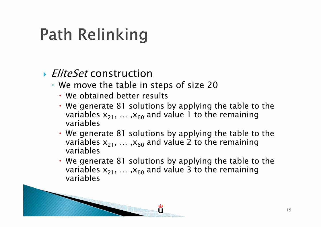
� EliteSet construction◦ We move the table in steps of size 20� We obtained better results

� We generate 81 solutions by applying the table to the variables x , … ,x and value 1 to the remaining variables x21, … ,x60 and value 1 to the remaining variables

� We generate 81 solutions by applying the table to the variables x21, … ,x60 and value 2 to the remaining variables

� We generate 81 solutions by applying the table to the variables x21, … ,x60 and value 3 to the remaining variables

19

� EliteSet construction◦ # solutions generated with this process:

� DSize=243⌈n/20⌉

◦ EliteSet is built choosing the best b solutions◦ EliteSet is built choosing the best b solutions

20

� Improvement is performed in two stagestwo stagestwo stagestwo stages1. Line search based on a single variable

� Grid size h=(u-l)/100

2. Simplex method2. Simplex method

� Not limited to the grid

21

� Improvement method: Line searches◦ For each variable i� We evaluate x+hei and x-hei, discarding the worst

valuevalue

◦ We order the variables i={1, … ,n} according to these values

22

xx-hei x+hei

� Improvement method: Line searches

1. ExploreExploreExploreExplore the first n/2 variables in the order that was previously calculated:

For each variable i, evaluateevaluateevaluateevaluate solutions with the form

� x+khei

� k=[-20,20]� k=[-20,20]

� l ≤ x+khei ≤ u

HOW?HOW?HOW?HOW? Randomly & using a first-improvement approach

23

xx-hei x+hei x+4heix-4hei

� Improvement method: Line searches

1. ExploreExploreExploreExplore the first n/2 variables in the order that was previously calculated:

For each variable i, evaluateevaluateevaluateevaluate solutions with the form

� x+khei

� k=[-20,20]� k=[-20,20]

� l ≤ x+khei ≤ u

HOW?HOW?HOW?HOW? Randomly & using a first-improvement approach

2. ReReReRe----evaluateevaluateevaluateevaluate the contribution of each variable, and re-order

� We explore again the first n/2 variables

3. RepeatRepeatRepeatRepeat it for 10 iterations, or until no further improvement is possible

24

� Improvement method: Simplex� Let x be the best solution found after the first stage

(line searches)

� We perturb the value of each variable:

� x=(x1, ... ,xi + α, ... ,xn)

� α is generated by a uniform probability in [-1,1]� α is generated by a uniform probability in [-1,1]

� The simplex method is applied to these solutions

25

� Relinking method◦ Straight linking

◦ We perform the linking between three solutions

� An initial solution, a� An initial solution, a

� Two guiding solutions, x and y

26

� Relinking method◦ Straight linking

y2 y

27

a

a1

a2

x1

x2

y1

x a(2k-1)

a(1)

a(k-1)

a(j)

a(k+1)

� Relinking method◦ We start at a=(a1,...,an)

◦ Firstly we evaluate solutions in the direction given by the vector from a to xby the vector from a to x

28

)(2

1)1(

...

)(1

1)2(

)(1

)1(

axaka

axk

aa

axk

aa

−+=−

−−

+=

−+=

� Relinking method:◦ The best solution is chosen from previous step, a(j)

◦ Then we evaluate solutions in the direction given by the vector from a(j) to ythe vector from a(j) to y

29

))((2

1)()22(

...

))((1

1)()1(

))((1

)()(

jayjaka

jayk

jaka

jayk

jaka

−+=−

−−

+=+

−+=

� Evolutionary Path Relinking (EvoPR)◦ [Resende y Werneck, 2004]

◦ EliteSet evolution

30

� EvoPR1. EliteSet construction

2. Do

3. Apply relinking method to solutions in EliteSet3. Apply relinking method to solutions in EliteSet

4. If no new solution can enter EliteSet → rebuild EliteSet

5. Until max number evaluations is reached

31

1. Obtain an EliteSet of b elite solutions.2. Evaluate the solutions in EliteSet and order them. Make NewSolutions = TRUE and GlobalIter=0.while ( NumEvaluations < MaxEvaluations ) do

3. Generate NewSubsets, which consists of the sets (a, x, y) of solutions in EliteSet that include at least one new solution. Make NewSolutions = FALSE and Pool = ∅.while ( NewSubsets ≠ ∅∅∅∅ ) do

4. Select the next set (a, x, y) in NewSubSets.5. Apply the Relinking Method to produce the sequence from a to x and y.6. Apply the Improvement Method to the best solution in the sequence. Let w be the improved solution. Add w to Pool.7. Delete (a, x, y) from NewSubsets

∈∈∈∈

32

7. Delete (a, x, y) from NewSubsetsend whilefor (each solution w ∈∈∈∈ Pool)

8. Let xw be the closest solution to w in EliteSetif ( f(w) < f(x1) or ( f(w) < f(xb) & d(w, xw)>dthresh) then

9. Make xw = w and reorder EliteSet10. Make NewSolutions = TRUE

end ifend for11. GlobalIter = GlobalIter +1If ( GlobalIter = MaxlIter or NewSolutions= FALSE)

12. Rebuild the RefSet. GlobalIter =0end if

end while

� Introduction

� Path Relinking

Experimental Experimental Experimental Experimental resultsresultsresultsresults� Experimental Experimental Experimental Experimental resultsresultsresultsresults

� Conclusions

33

� Benchmark◦ 19 functions with known optimum

� 6 from CEC’2008

� 5 shifted functions� 5 shifted functions

� 8 hybrid functions

◦ Requirements

� 5 dimensions: D={50,100,200,500,1000}

� 25 executions per algorithm and function

� Maximum number of evaluations: 5000D

34

� Requirements◦ Experiments report the error:

� f (x)-f (op)

� x is the best solution found� x is the best solution found

� op is the optimum of the function

35

� Results◦ Constructive methods

� We compare our constructive method with the method described in [Duarte et al., 2010]method described in [Duarte et al., 2010]

� 1000 constructions

� F3, F8, F13

36

50505050 100100100100 200200200200 500500500500 1000100010001000

Frequency 5.3E10 1.1E11 2.7E11 7.3E11 1.5E12

Taguchi 3.7E103.7E103.7E103.7E10 6.0E106.0E106.0E106.0E10 1.3E111.3E111.3E111.3E11 3.7E113.7E113.7E113.7E11 7.6E117.6E117.6E117.6E11

� Results◦ Improvement methods

� We test several methods that were reported as the best ones for global optimization (Hvattum et al., 2010)ones for global optimization (Hvattum et al., 2010)

� 100 constructions (Taguchi) + Improvement + Simplex

� F3, F13, F17

37

50505050 100100100100 200200200200 500500500500 1000100010001000

CS [Kolda et al., 2003] 8.2E13 2.8E14 8.0E14 1.7E15 2.1E16

SW [Solis y Wets, 1981] 3.2E10 6.2E10 1.4E11 1.9E11 8.4E11

TLS [Duarte et al., 2010] 1.7E9 5.2E9 1.3E10 2.3E11 9.7E10

TSLS 1.8E31.8E31.8E31.8E3 4.1E34.1E34.1E34.1E3 1.2E41.2E41.2E41.2E4 2.2E102.2E102.2E102.2E10 4.6E44.6E44.6E44.6E4

� Results◦ Path relinking methods

� Static PR and Evolutionary PR

� F3, F13, F17� F3, F13, F17

38

PRPRPRPR EvoPREvoPREvoPREvoPR

|ES| 10101010 4444 8888 12121212

50 6.2E1 7.6E1 5.2E1 7.9E1

100 1.3E2 1.8E2 2.5E2 6.1E2

200 5.2E2 4.8E2 9.8E2 1.7E3

500 2.3E3 1.6E3 2.7E3 4.3E3

1000 5.8E3 3.9E3 6.7E3 8.9E3

Average 1.7E3 1.3E31.3E31.3E31.3E3 2.1E3 3.1E3

� Final experiment◦ 19 functions, 5 dimensions, 25 runs per method

and function, 5000D evaluations

◦ Average error is reported◦ Average error is reported

39

DEDEDEDE CHCCHCCHCCHC GGGG----CMACMACMACMA----ESESESES

STSSTSSTSSTS EvoPREvoPREvoPREvoPR

50 3.1E0 2.4E5 1.0E2 1.3E2 1.4E1

100 3.0E1 5.8E6 2.3E2 6.2E2 6.3E1

200 3.5E2 1.4E8 5.4E2 2.8E3 1.9E2

500 3.7E3 3.4E9 2.2E255 1.9E4 3.7E2

1000 1.5E4 2.0E10 - 1.4E4 1.2E3

Average 3.7E3 4.8E9 5.6E254 7.2E3 3.7E2

� Introduction

� Path Relinking


� ConclusionsConclusionsConclusionsConclusions

40

� Path Relinking for Global Optimization◦ Constructive method based on

� Fractional experiment design

� Diverse solutions� Diverse solutions

◦ Linking strategy with more than two solutions

◦ Improvement method

� Line search with grid

� First-improvement approach

� Random evaluation of points

41

� A balance between...◦ Solution space exploration

◦ Limited number of evaluations

� Competitive method compared with state of � Competitive method compared with state of the art◦ EvoPR performs better in high dimensions

42

ThankThankThankThank youyouyouyou!!!!

Path relinking for high dimensional continuous optimization

Education

Transcript of Path relinking for high dimensional continuous optimization