Scholars' Mine Scholars' Mine

Masters Theses Student Theses and Dissertations

Fall 2012

Path planning for general mazes Path planning for general mazes

Grant Gilbert Arthur Rivera

Follow this and additional works at: https://scholarsmine.mst.edu/masters_theses

Part of the Electrical and Computer Engineering Commons

Department: Department:

Recommended Citation Recommended Citation Rivera, Grant Gilbert Arthur, "Path planning for general mazes" (2012). Masters Theses. 6944. https://scholarsmine.mst.edu/masters_theses/6944

This thesis is brought to you by Scholars' Mine, a service of the Missouri S&T Library and Learning Resources. This work is protected by U. S. Copyright Law. Unauthorized use including reproduction for redistribution requires the permission of the copyright holder. For more information, please contact scholarsmine@mst.edu.

PATH PLANNING FOR

GENERAL MAZES

by

GRANT GILBERT ARTHUR RIVERA

A THESIS

Presented to the Faculty of the Graduate School of the

MISSOURI UNIVERSITY OF SCIENCE AND TECHNOLOGY

In Partial Fulfillment of the Requirements for the Degree

MASTER OF SCIENCE IN ELECTRICAL ENGINEERING

2012

Approved by

Kurt Kosbar, Advisor

Donald Wunsch II

Maciej Zawodniok

iii

ABSTRACT

Path planning is used in, but not limited to robotics, telemetry, aerospace, and

medical applications. The goal of the path planning is to identify a route from an

origination point to a destination point while avoiding obstacles. This path might not

always be the shortest in distance as time, terrain, speed limits, and many other factors

can affect the optimality of the path. However, in this thesis, the length, computational

time, and the smoothness of the path are the only constraints that will be considered with

the length of the path being the most important. There are a variety of algorithms that

can be used for path planning but Ant Colony Optimization (ACO), Neural Network, and

A* will be the only algorithms explored in this thesis.

The problem of solving general mazes has been greatly researched, but the

contributions of this thesis extended Ant Colony Optimization to path planning for

mazes, created a new landscape for the Neural Network to use, and added a bird’s eye

view to the A* Algorithm. The Ant Colony Optimization that was used in this thesis was

able to discover a path to the goal, but it was jagged and required a larger computational

time compared to the Neural Network and A* algorithm discussed in this thesis. The

Hopfield-type neural network used in this thesis propagated energy to create a landscape

and used gradient decent to find the shortest path in terms of distance, but this thesis

modified how the landscape was created to prevent the neural network from getting

trapped in local minimas. The last contribution was applying a bird’s eye view to the A*

algorithm to learn more about the environment which helped to create shorter and

smoother paths.

iv

ACKNOWLEDGMENTS

I’d like to thank my advisor, Dr. Kurt Kosbar, for providing me the opportunity to

do research. I’m extremely grateful for his guidance through my graduate courses,

helping me prepare, sending me to conferences, and all of his advice with my thesis. I

would also like to thank my committee members, Dr. Donald Wunsch II and Dr. Maciej

Zawodniok, my family and friends who have always believed in me and encouraged me,

and my girlfriend, Amber, who wouldn’t let me procrastinate, come over, or play video

games until I made substantial progress on my school work and thesis.

v

TABLE OF CONTENTS

Page

ABSTRACT ...................................................................................................................... iii

ACKNOWLEDGMENTS ................................................................................................ iv

LIST OF ILLUSTRATIONS ........................................................................................... vii

LIST OF TABLES ............................................................................................................ ix

SECTION

1. INTRODUCTION ..............................................................................................1

2. ACO LITERATURE REVIEW ..........................................................................5

3. ACO IMPLEMENTATION ...............................................................................6

3.1. PARAMETERS ...................................................................................6

3.1.1. Population Size .....................................................................6

3.1.2. Pheromone Decay .................................................................6

3.1.3. Heuristic Weight ...................................................................6

3.1.4. Pheromone Weight ................................................................7

3.1.5. Pheromone Intensity .............................................................7

3.2. TOUR CONSTRUCTION ...................................................................8

3.3. RESULTS ............................................................................................9

3.4. CONCLUSION ..................................................................................10

4. NEURAL NETWORK LITERATURE REVIEW ...........................................12

5. NEURAL NETWORK IMPLEMENATION ...................................................13

5.1. PROPAGATION ...............................................................................13

5.2. RESULTS ..........................................................................................16

vi

5.3. CONCLUSION ..................................................................................21

6. A* LITERATURE REVIEW ...........................................................................22

7 A* IMPLEMENTATION ..................................................................................23

7.1. BIRD’S EYE VIEW ..........................................................................23

7.2. RESULTS ..........................................................................................25

7.3. CONCLUSION ..................................................................................29

8. CONCLUSION .................................................................................................31

BIBLIOGRAPHY .............................................................................................................32

VITA .................................................................................................................................35

vii

LIST OF ILLUSTRATIONS

Page

Figure 3.1. Ant System .......................................................................................................9

Figure 3.2. Elitist Ant System .............................................................................................9

Figure 3.3. Rank Based Ant System .................................................................................10

Figure 3.4. AS Simulated 5 Times ....................................................................................10

Figure 5.1. Initial Energy with Target at (3,3) ..................................................................13

Figure 5.2. Elevation of Figure 5.1. at (3,3) .....................................................................13

Figure 5.3. Energy After First Propagation ......................................................................14

Figure 5.4. Elevation of Figure 5.3. ..................................................................................15

Figure 5.5. Final Energy ...................................................................................................16

Figure 5.6. Final Elevation ................................................................................................16

Figure 5.7. First Maze .......................................................................................................18

Figure 5.8. Second Maze ..................................................................................................18

Figure 5.9. Third Maze .....................................................................................................19

Figure 5.10. First Maze 2D Elevation ...............................................................................19

Figure 5.11. First Maze 3D Elevation ...............................................................................19

Figure 5.12. Second Maze 2D Elevation ..........................................................................19

Figure 5.13. Second Maze 3D Elevation ..........................................................................20

Figure 5.14. Third Maze 2D Elevation .............................................................................20

Figure 5.15. Third Maze 3D Elevation .............................................................................20

Figure 7.1. Dijkstra’s Test Maze .......................................................................................26

Figure 7.2. A* Test Maze .................................................................................................26

viii

Figure 7.3. A* W/Bird’s Eye Test Maze ..........................................................................26

Figure 7.4. Dijkstra’s First Maze ......................................................................................26

Figure 7.5. A* First Maze .................................................................................................27

Figure 7.6. A* W/Bird’s Eye First Maze ..........................................................................27

Figure 7.7. Dijkstra’s Second Maze ..................................................................................27

Figure 7.8. A* Second Maze .............................................................................................27

Figure 7.9. A* W/Bird’s Eye Second Maze .....................................................................28

Figure 7.10. Dijkstra’s Third Maze ...................................................................................28

Figure 7.11. A* Third Maze .............................................................................................28

Figure 7.12. A* W/Bird’s Eye Third Maze ......................................................................28

ix

LIST OF TABLES

Page

Table 3.1. ACO Simulated Five Times Result .................................................................10

Table 5.1. Neural Network Simulated Five Times Result ................................................20

Table 7.1. A* Simulated Five Times Result .....................................................................29

1. INTRODUCTION

There are various searching techniques, algorithms, and path planning problems

such as Hybrid Binary Particle Swarm Optimization (HBPSO) algorithm for a Multi-

vehicle Search Area coverage problem [1], Differential Evolution Particle Swarm

Optimization (DEPSO) algorithm for clustering [2], and Adaptive Critic Design for the

generalized maze problem [3-4]. This thesis will focus only on the generalized maze

problem using Ant Colony Optimization (ACO), Neural Networks (NN), and A*

(pronounced A-Star) algorithms.

Ant Colony Optimization (ACO) [5-13] was the first algorithm considered for this

thesis. There are many different versions of ACO which have been used for problems

such as routing, assignment, scheduling, subset, and others [5, 9]. Most of the problems

ACO is used for are NP-hard problems [5, 9] and most notably the traveling salesman

problem (TSP) [5, 9-11]. This thesis expanded ACO to path planning for mazes. Since

the goal of the TSP is to be able to find the shortest path by traveling to each city once

and returning to the starting city, finding the shortest path through a maze should be

similar.

It is important to note that typically ACO is applied to small scale TSP not

necessarily to make strides in solving the TSP problem but more so to be used as a

benchmark to show how that version of ACO can be used as an optimization tool and

possibly how it compares to other algorithms [5, 9-11]. Using TSP as a benchmark is not

limited to ACO or even to small scale TSP problems, Mulder and Wunsch [14] not only

compare multiple algorithms but compare how they scale by using large scale TSP

2

problems (1000+ cities). It is also important to note that TSP problems, especially large

scale TSP problems, are approached by heuristic methods [14-17]. The heuristic uses

special knowledge about the problem and incorporates it to help simplify the problem or

allows certain assumptions to be made which in turn helps to solve the problem quicker.

Since this is usually an estimate, the result might not always be optimal but should return

a close to optimal solution as long as the heuristic was chosen appropriately. This can

most be seen by the algorithms discussed in this paper especially in Section 7.2 where

Dijkstra’s algorithm, which doesn’t have a heuristic [18-20], is compared to A*, which is

the same algorithm but with a heuristic [18-22].

The ability of the algorithm to learn over time by using the collective swarm

knowledge of how the ants have explored previously and its ability to be used for real-

time environments, as opposed to needing a simulated model of the environment, made

this algorithm desirable. Using a simulated model of the environment to plan a path

might not be possible for unknown environments or environments that are constantly

changing. Since the path created depended on a stochastic process of the algorithm, the

randomization caused the path to be very jagged. The quality of the path and the

computational time in creating the path were also affected by what the parameters for

ACO were set to. This is covered in more detail in Section 3.1. One method that might

have improved the performance would have been to make the ants stubborn [12, 13].

A new neural network method for path planning created by Zhong et al. [23] was

the next algorithm to be employed. Unlike ACO, this algorithm could be used in

environments that change with the respect to time, had a much smaller computational

time, and did not rely on parameters or randomization. For the environments studied in

3

this thesis, the algorithm tended to become stuck in local minima. Section 5.1 describes a

way to improve the algorithm to avoid this problem. While the algorithm was superior to

ACO for the problems investigated, it generated paths that had zero radius or sharp turns.

It was not immediately obvious how one would modify the neural network algorithm to

favor smoother paths, which motivated us to explore other algorithms. Instead of looking

at other algorithms, further research into biasing neural networks to avoid obstacles might

have yielded better results [24].

A* [18-22] was studied in Section 6 and 7 of this thesis because of its known

performance and popularity as a path planning algorithm. A* finds an optimal path in

terms of distance but is generally not used for real-time environments since the

environment needs to be static, or unchanging. The A* algorithm was improved by using

a “bird’s eye view”. This allowed the algorithm to generate smoother paths, which could

possibly allow the robot to traverse the paths faster, and avoids the need to have as many

sharp turns. For environments that are constantly changing, a modified version of A*

called LRTA* can be used [25].

The environments for each algorithm were all modeled using discrete space by

creating an evenly spaced binary matrix where nodes that contained a value of one were

considered travelable and nodes with a zero represented an obstacle. This method was

chosen for simplicity. Since the nodes were discretely spaced instead of being

continuous, the paths were not as good as they could have been. Some of the issues with

these paths include traveling too close to obstacles, creating 90 degree angles with small

turning radius, and producing a jagged path.

4

Traveling too close to obstacles could cause the mobile robot to hit an obstacle or

could lead to having to make sharper turns. Having sharp turns or 90 degree angles with

small turning radius could cause longer traveling time or could generate turns that are not

feasibly possible for the mobile robot. Jagged paths might slow down the robot and

could be difficult to follow. Many of these algorithms are also based on the length of the

path instead of the time required to travel the path. Therefore, creating or modifying an

algorithm that could produce a path without these issues was desired. Having more

nodes to represent the environment could have also helped with some of these problems

and would have made the paths seem more continuous but increasing the number of

nodes also increases the computational time since there will be more nodes that would

have to be traveled through and more searching done by the algorithms.

All three algorithms (ACO, NN, and A*) will be covered respectively in sections

2-7. Each algorithm will be broken into two different sections, a literature review part

and an implementation part. The literature review section will give a brief explanation of

each algorithm. The implementation section will focus on modifications made by this

thesis, issues discovered with the algorithm, and the results for the algorithm.

5

2. ACO LITERATURE REVIEW

Ant Colony Optimization simulates the behavior of biological ants. For path

planning, this behavior is that of the foraging ants. Dorigo [5] developed this foraging

behavior which he called the Ant System (AS). Foraging ants randomly explore in

search for food. Once a food source is found, the ants deposit pheromone from the food

back to the colony. This pheromone trail attracts other ants. Since only one pheromone

deposit has been made, the pheromone level will be weak and will have limited attraction

to other ants. This means that most ants will still randomly explore for food instead of

following the initial ant’s path.

Over time as ants lay pheromone across the paths, the pheromone levels will

increase. Even though each ant’s path is different, there is generally some overlapping

for certain areas especially where the path is the best. Since multiple ants cross this

section, pheromone is deposited at a much quicker rate. The areas with the largest amount

of pheromone attract the most ants. This reduces the amount of exploration and causes

the ants to exploit the pheromone paths. As time passes, pheromone slowly decays which

weakens the attraction and if pheromone is not replenished, the path will disappear. This

allows the longer, rarely traveled paths to be forgotten. Eventually the ants will converge

on the shortest path.

6

3. ACO IMPLEMENTATION

3.1. PARAMETERS

In order to replicate the foraging behavior artificially, all of the parameters

(population size, pheromone decay rate, pheromone weight, heuristic weight, and

pheromone intensity) need to be optimized. However, since optimizing these parameters

is a nonlinear multivariable problem, finding an optimized value is difficult. The

methods typically used to optimize these parameters are with trial-and-error where the

length and computational time is checked with each parameter modification or to use

another optimizing algorithm. Both of these methods add to the computational time, and

the values found for each parameter will have to constantly change as the environment

changes. Trial-and-error was used in this thesis.

3.1.1. Population Size. Having a large population size gives a more thorough

search but also increases computational time due to more searches being done. The

larger the environment, the larger the population size will have to be to explore it.

3.1.2. Pheromone Decay. The pheromone decay rate determines the rate at

which paths are forgotten. Having poor paths remain in the environment to be explored

over and over again is a waste of computational time, however, if the decay rate is too

fast, it might be possible to forget an optimal path due to the path not remaining long

enough for ants to deposit enough pheromone to be biased to it.

3.1.3. Heuristic Weight. The heuristic weight is the bias to the goal based on the

heuristic information. The heuristic information is the distant to the goal and is

calculated using the Euclidean Distance Formula. If the value for the heuristic weight is

7

too low then there will be no feedback to the goal and the ants’ paths will depend only on

the pheromone quantity. If the heuristic weight is too high then there will be no

exploration and will only be a greedy search. The ants might also get trapped.

3.1.4. Pheromone Weight. The pheromone weight represents how strongly the

pheromone influences the ant’s behavior. If it’s too low then the searching will be based

only on the heuristic information but if the heuristic weight is low too when the

pheromone weight is low then the ants will randomly explore. When the pheromone

weight is too high, there will be very little exploration. Instead, previous discovered

paths will be exploited.

3.1.5. Pheromone Intensity. The amount of pheromone applied to each node is

the pheromone intensity. The pheromone quantity of each node is stored in matrix. The

pheromone intensity is the only parameter that has an equation to set it. All nodes need

to start with an equal amount of pheromone. It should be equal so there is no initial bias.

If the pheromone level is initialized too low the ants will converge too quickly and an

optimal path will not be found. When the pheromone intensity is too high, there will be

many wasted iterations waiting for the pheromone to evaporate enough for the ants’ paths

to be biased by the pheromone levels since the ants deposit only a small amount of

pheromone. Pheromone intensity can be determined by the following equation which is

still estimated:

*0f

m=τ

Where:

− 0τ is the pheromone intensity

− m is the number of ants

8

− *f is an estimation of the optimal value, or distance, of the shortest path for the

function.

3.2. TOUR CONSTRUCTION

Ants use a probabilistic selection based on the quantity of the pheromone and the

heuristic information to decide which node to travel to. The ACO literature [5-9] does

not describe how these probabilities were applied so the probability mass function was

used. In order to prevent the ants from traveling through a single node multiple times

during a single trip, a revisiting prevention method was created.

Since obstacles have a pheromone value of zero to prevent being traveled to, a

temporary pheromone matrix was created to set the pheromone level to zero for

previously traveled to nodes. A temporary matrix is initialized as an exact copy of the

actual pheromone values at the start of each ant’s tour. A temporary matrix is used

because the actual pheromone values still need to be used for future explorations. Each

time an ant travels to a new node, the temporary pheromone value will be set to zero to

prevent the ant from staying at that node or returning to it but this could cause the ant to

be able to trap itself by being surrounded by nodes with a pheromone level of zero.

Therefore, any time the current node and surrounding nodes are zero, the temporary

pheromone matrix is re-initialized with the same values as the actual pheromone matrix.

Since it is still possible to visit a node more than once in a tour, a check is done to see

when the first and last time a repeated node is visited. All nodes in-between the first and

last time are removed from the tour.

9

3.3. RESULTS

There are many different versions of ACO but only three of them were tested: Ant

System (AS) [5, 9] Figure 3.1., Elitist Ant System (EAS) [5, 9] Figure 3.2., and Rank

Based Ant System (ASrank) [5, 9] Figure 3.3. The computational time and paths change

each time the algorithms are used. This can be seen from Figure 3.4. where Ant System

is simulated five times. Do to these changes, the average and standard deviation for

computational time and path lengths of each algorithm for five trials are recorded in

Table 3.1. The parameters were optimized through trial-and-error for AS, and then, those

same parameters were used for ASrank and EAS.

Figure 3.1. Ant System Figure 3.2. Elitist Ant System

10

Figure 3.3. Rank Based Ant System Figure 3.4. AS Simulated 5 Times

Table 3.1. ACO Simulated Five Times Result

Name Average

Computational

Time

Standard

Deviation of

Time

Average

Path Length

Standard

Deviation of

Path Length

Ant System 48 minutes

27.2134 seconds

7 minutes

40.5503 seconds

309.4074 5.2346

Elitist Ant

System

48 minutes 26.4

seconds

3 minutes

53.0489 seconds

309.4476 10.8615

Rank Based Ant

System

54 minutes

11.0868 seconds

5 minutes

28.6259 seconds

305.1532 6.1198

3.4. CONCLUSION

Upon implementation of the algorithm, it was discovered that, due to the

randomization and needing to optimize the parameters, paths were jagged and were not

optimal in terms of distance. The over-all path as far as which areas were best to travel

through was optimal, but how it traveled through those areas was far from optimal. Most

of the paths contained “zig-zags” instead of being a straight line. The ants use a

11

probabilistic selection based on the quantity of pheromone and the heuristic information

when deciding which node to travel to which causes the randomization. This

randomization is good for finding different paths but bad for being able to create an

optimal path and causes the paths to not be smooth.

Even though the algorithm learned over time to improve its path, it would not

work in a real-time environment where the environment constantly changes because of

parameter changes and needing time to learn. It would work best in an environment

where it could first be trained offline and then when a change in the environment

occurred it would need to have time to learn the new environment. For each change, the

parameters would need to be re-optimized, but I am unaware of a formula to optimize

these parameters. Trial-and-error or another optimizing algorithm would have to be used

instead which both methods would add to computational time. It took ACO on average

over 48 minutes computationally to create the path not counting time spent for trial-and-

error. It took the neural network and A* only seconds to solve the same maze and they

were both able to find shorter paths than ACO. The time and paths might have been

improved by making the ants stubborn. Stubborn ants can differentiate their own

pheromone compared to other ants’ pheromone and will be biased more to their own

pheromone which helps to create diversity in the paths [12, 13].

12

4. NEURAL NETWORK LITERATURE REVIEW

Neural networks have successfully been applied to path planning by using neural

networks to recognize patterns for a wall following algorithm [26], using spiking neural

networks with dynamic memory for autonomous mobile robots [27], and using Hopfield

neural networks for direction in a direction map [28]. A different collision-free path

planning algorithm that uses a Hopfield-type neural network that does not need any

previous knowledge of the search space or learning procedures was purposed by Zhong et

al. [23]. This was accomplished by treating the target as an energy source. The energy

was propagated in a square formation from the target to all of the connecting neurons

which represent free spaces in the search space. The neurons not connected to other

neurons represented obstacles and thus, were never given any energy. This energy was

then used as a landscape in which the highest energy, the target, represented the peak of

the landscape while the obstacles represented the lowest elevation of the landscape. By

traveling up the steepest gradient from the starting point, an optimal or close to optimal

path was found in terms of shortest distance. The main ways this paper differs from the

paper purposed by Zhong et al. [23] was by creating a separate landscape instead of using

the actual energy and by propagating in a cross fashion instead of a square formation.

13

5. NEURAL NETWORK IMPLEMENTATION

5.1. PROPAGATION

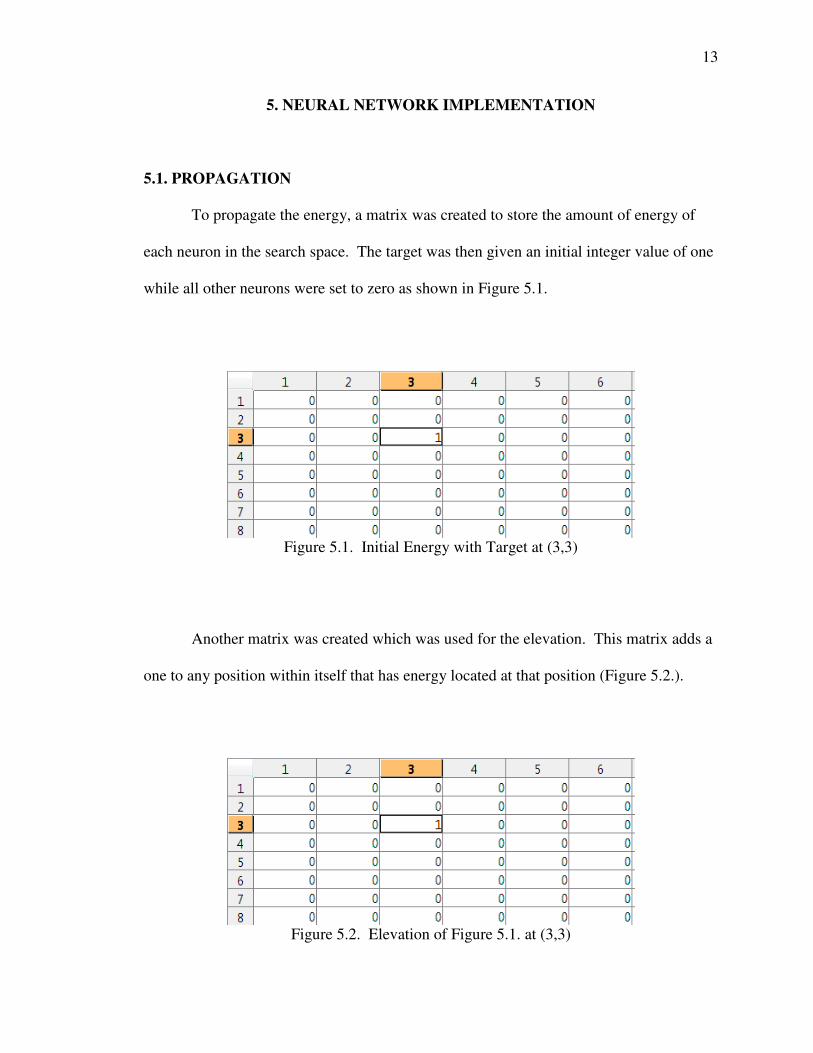
To propagate the energy, a matrix was created to store the amount of energy of

each neuron in the search space. The target was then given an initial integer value of one

while all other neurons were set to zero as shown in Figure 5.1.

Figure 5.1. Initial Energy with Target at (3,3)

Another matrix was created which was used for the elevation. This matrix adds a

one to any position within itself that has energy located at that position (Figure 5.2.).

Figure 5.2. Elevation of Figure 5.1. at (3,3)

14

The energy matrix values were propagated by shifting the energy up one node,

down one node, left one node, and to the right one node. These shifts were then added

back into the original energy matrix after being multiplied by a weight. The weights for

diagonal movements should have been given a value of 0.5 and all horizontal and vertical

movements should have a weights of 1 [23], but since the energy was not used as the

landscape, all weights were set to 1. A check was then done to see if any of these nodes

with energy were unconnected neurons. If they were unconnected, the energy was reset

to zero for that particular neuron (Figure 5.3.).

Figure 5.3. Energy After First Propagation

The main difference from this method and the method purposed in the neural

network paper [23] was that only the neighbors above, below, to the left, and to the right

were allowed to propagate, not diagonal, and since energy wasn’t used for the landscape,

there was no additional energy deposited to the target after each iteration. This can be

seen from the following equations:

15

shiftrightshiftleftshiftdownshiftupM

MMshiftright

MMshiftleft

MMshiftdown

MMshiftup

ji

jijiji

jijiji

jijiji

jijiji

____

_

_

_

_

,

,1,,

,1,,

1,,,

1,,,

+++=

+=

+=

+=

+=

−

+

+

−

Where:

M = The matrix

R = The number of rows in the matrix

C = The number of columns in the matrix

Ri <<1

Cj <<1

After the energy propagation, the elevation matrix added a one to itself for any

node that contained energy (Figure 5.4.).

Figure 5.4. Elevation of Figure 5.3

This process continued until a certain number of iterations had passed or until

the energy had propagated from the target to the starting point (Figures 5.5.-5.6.).

16

Figure 5.5. Final Energy

Figure 5.6. Final Elevation

The target, which should have the largest value for gradient decent to work, is

located at (3,3). Figure 5.6. has the largest value at the target at (3,3) but in Figure 5.5.

the largest value is at (4,4) which is not the correct target which is why the landscape in

Figure 5.6. had to be used instead of the energy. Iterations were used to prevent an

infinite loop just in case there was no solution to the search space such as obstacles

completely surrounding the target space preventing any movement to it.

5.2. RESULTS

The results of the simulations are illustrated in Figures 5.7.-5.15. These paths

almost identically match those from the neural network paper [23] even though the

weights, landscape, and propagation were different from the purposed method. Another

17

main difference was instead of plotting the path on the vertices of the grid they were

plotted on the center of the free space squares. Each simulation took less than a second.

Propagating energy from the target to the starting point as purposed from Zhong

et al. [23] did not always create a peak at the target in which case the path never traveled

to the target. They added an additional amount to the target, but since the propagation

expands exponentially, adding an additional amount did not solve the problem. Instead,

the target had to be manually set once the propagation was done to have the most energy.

Because energy is propagated from each neighbor, any neuron next to an obstacle (an

unconnected neuron) did not receive as much energy from its neighbors. This was

desired to keep the robot away from the obstacles but this also caused multiple peaks to

form which the path would get stuck on and was also the reason why the target was not

always the maximum point. No where in the paper did it state how their algorithm

prevented these problems.

Using a separate landscape based on if any energy was present at each specific

location was used instead. This method ensured the target was always at the maximum

and that all the obstacles were minimums. Propagating in a square formation as in the

replicated paper caused certain areas to not change in elevation for a few steps. When

looking at the surrounding neighbors, it appeared that the neuron was a peak even though

at least one neighbor had the same value. So instead of making a sloping elevation, it

made a stair-like elevation. This could be fixed in the code where the robot always has to

choose a new neuron to travel to, but in certain dynamic situations, it might be better for

the robot to wait where it is instead of moving. Propagating in a cross fashion solved this

problem by evenly disperse the elevation of the landscape which made it sloped. The

18

weights recommended were then used in the computing of the path instead of in

propagating the energy even though some weights were also used in the propagation.

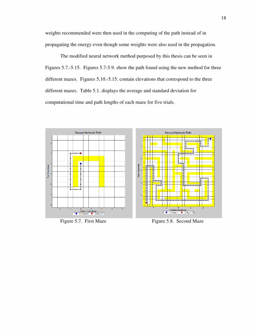
The modified neural network method purposed by this thesis can be seen in

Figures 5.7.-5.15. Figures 5.7-5.9. show the path found using the new method for three

different mazes. Figures 5.10.-5.15. contain elevations that correspond to the three

different mazes. Table 5.1. displays the average and standard deviation for

computational time and path lengths of each maze for five trials.

Figure 5.7. First Maze Figure 5.8. Second Maze

19

Figure 5.9. Third Maze Figure 5.10. First Maze 2D Elevation

Figure 5.11. First Maze 3D Elevation Figure 5.12. Second Maze 2D Elevation

20

Figure 5.13. Second Maze 3D Elevation Figure 5.14. Third Maze 2D Elevation

Figure 5.15. Third Maze 3D Elevation

Table 5.1. Neural Network Simulated Five Times Result

Name Average

Computational

Time

Standard

Deviation of

Time

Average

Path Length

Standard

Deviation of

Path Length

First Maze 0.8061 seconds 0.0134 seconds 16 0.0

Second Maze 0.9442 seconds 0.0790 seconds 124 0.0

Third Maze 1.2730 seconds 0.0558 seconds 252.51 0.0

21

5.3. CONCLUSION

By propagating energy through the connected neurons, a landscape was created in

which the target was at the peak while the obstacles were at the bottom. Even though a

different method was used in creating the landscape, propagating the energy, and using

the weights, the results were very similar to what Zhong et al. [23] found. This is most

likely because the overall idea of how the neural network is suppose to work by traveling

up the gradient to the target since the target is the largest while the starting point is the

smallest besides for obstacles was exactly the same. In their paper, they did not fully

describe their process well enough for it to be replicated using the exact same method as

them.

The neural network was able to solve each maze substantially faster than ACO.

Even the path discovered was smoother and had a better result in terms of distance.

Every path could be exactly replicated since there was no randomization or probabilities

used. There were no parameters that needed to be optimized so the exact algorithm could

be used on any path planning problem. Since the gradient decent method was used, the

only way to modify the paths to become smoother would be to improve the elevation.

The original method [23] was supposed to work on dynamic problems and keep a slight

distance from all obstacles but the method actually employed will work only on static

environments and has no distant requirement from obstacles as long as it does not collide

with them. Since the elevation depends on the environment, modifying the elevation to

get smoother paths would be difficult. As stated in the introduction, adding an extra

biasing to the neural network could possibly solve this problem [24].

22

6. A* LITERATURE REVIEW

The A* algorithm was chosen for its popularity, its ability to find an optimal

solution, and its use in navigation systems and video games [18-22]. A*’s ability for its

paths to be replicated by constantly finding the optimal solution and for the search

algorithm to be easily modified made this algorithm desirable for path planning. A*,

however, will only work for static environments, environments that do not change, since

all obstacles and costs need to be known.

A* is a combination of both an exhaustive search, guaranteed to find the optimal

path but will typically require a large amount of computational time, and a greedy search,

directs the search towards the goal and is generally faster but will not usually find the

optimal solution [18-22]. The movement cost, a known cost from the starting point to get

to its current location, is the exhaustive part. The heuristic, an estimation of the distance

from its current location to the desired ending location, is the greedy part [18-22]. Since

A* is a combination of each, the algorithm is guaranteed that an optimal path will be

found and usually in a faster time than an exhaustive search.

There are numerous ways to calculate these costs. Which way works the best

depends on the method of travel and the desired speed and accuracy of the algorithm. If

only horizontal and vertical movements are allowed, the Manhattan Distance Formula

should work the best for accuracy, but if movement in all directions is allowed, then the

Euclidean Distance Formula would most likely be a better option [19-21]. Other methods

and situations for choosing the correct heuristic are thoroughly covered by Amit [18]. A*

without the heuristic part is known as Dijkstra’s algorithm [18-20].

23

7. A* IMPLEMENTATION

7.1. BIRD’S EYE VIEW

A* consists of two lists, an open-list and a closed-list. The open-list contains a

list of nodes that can currently be traveled to and the closed-list contains all the nodes

already traveled to [18-22]. The typical version of A* checks all adjacent nodes from its

current location and adds them to the open-list as long as they are not obstacles or already

on the open or closed list. The movement cost is then calculated from its current location

for all adjacent nodes that are free of obstacles. If this new movement cost is lower than

the previous calculated one, then that becomes the new value for the movement cost and

current node is remembered as the best way to get to that node. The following equation

uses the Euclidean Distance Formula for calculating the movement cost.

22 )()( cncncn ccrrGG −+−+=

Where:

− nG movement cost of the adjacent node.

− cG movement cost of the current node.

− nr row coordinate of the adjacent node.

− cr row coordinate of the current node.

− nc column coordinate of the adjacent node.

− cc column coordinate of the current node.

24

The heuristic cost will also be calculated but only for the adjacent nodes that are free

of obstacles and where the heuristic has yet to be calculated since the heuristic cost will

never change. The Euclidean Distance Formula was used in the following heuristic cost

equation.

22 )()( nfnfn ccrrH −+−=

Where:

− nH heuristic cost of the adjacent node.

− fr row coordinate of the desired ending location.

− nr row coordinate of the adjacent node.

− fc column coordinate of the desired ending location.

− nc column coordinate of the adjacent node.

The movement and heuristic costs are added together for each node on the open list,

and the node with the lowest overall cost will become the new current node.

nnn HGF +=

Where:

− nF fitness cost of the adjacent node.

− nG movement cost of the adjacent node.

− nH heuristic cost of the adjacent node.

This process is repeated until the desired ending location is reached.

25

Instead of using the adjacent nodes, a bird’s eye view was implemented. The

bird’s eye view was created by first checking the adjacent nodes for obstacles. If an

obstacle was found in any of the adjacent nodes, then the original A* algorithm was used.

However, if there are not any obstacles, then the unchecked adjacent nodes from the

original adjacent nodes are checked. This square-formation expansion is continued until

at least one obstacle is found and all nodes are checked from that square formation. The

outer parameter nodes of this square are the only nodes added to the open-list. The rest

of the A* algorithm works the same.

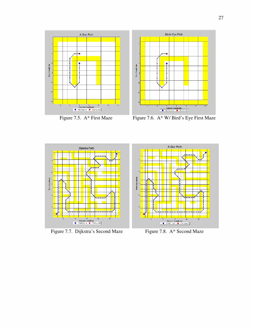
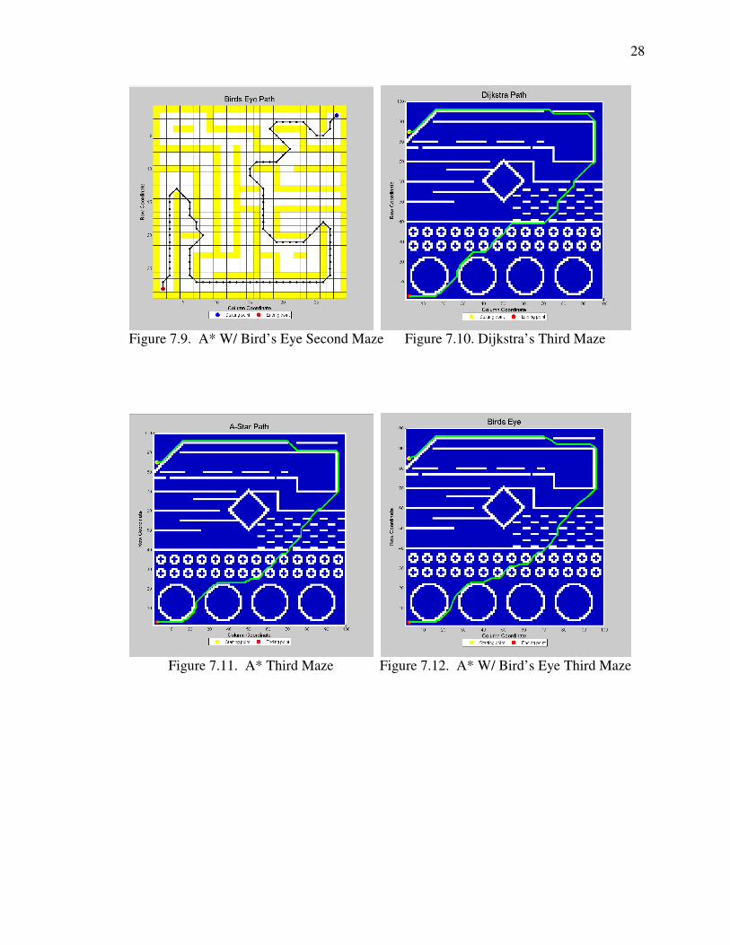
7.2. RESULTS

Using the bird’s eye view method sometimes lowered the computational time

required to find the shortest path but some mazes it also increased the time. It was also

able to find a better path for certain mazes. These results can be seen from Figures 7.1-

7.12 and Table 7.1. By having a larger viewing area for creating a path, allowed the

paths to be more direct and even though not used in this thesis, provided knowledge if

there was enough room for arc style turns to be used. The rest of the algorithm’s

searching procedure was the same as the original A*.

26

Figure 7.1. Dijkstra’s Test Maze Figure 7.2. A* Test Maze

Figure 7.3. A* W/ Bird’s Eye Test Maze Figure 7.4. Dijkstra’s First Maze

27

Figure 7.5. A* First Maze Figure 7.6. A* W/ Bird’s Eye First Maze

Figure 7.7. Dijkstra’s Second Maze Figure 7.8. A* Second Maze

28

Figure 7.9. A* W/ Bird’s Eye Second Maze Figure 7.10. Dijkstra’s Third Maze

Figure 7.11. A* Third Maze Figure 7.12. A* W/ Bird’s Eye Third Maze

29

Table 7.1. A* Simulated Five Times Result

Name Average

Computational

Time

Standard

Deviation of

Time

Average

Path Length

Standard

Deviation of

Path Length

Dijkstra

Test Maze

0.0348 seconds 0.0063 seconds 9.65685 0.0

A*

Test Maze

0.0164 seconds 0.0087 seconds 9.65685 0.0

A* W/ Bird-Eye

Test Maze

0.0136 seconds 0.0158 seconds 9.18204 0.0

Dijkstra

First Maze

0.0230 seconds 0.0045 seconds 14.2426 0.0

A*

First Maze

0.0142 seconds 0.0072 seconds 14.2426 0.0

A* W/ Bird-Eye

First Maze

0.0224 seconds 0.0222 seconds 14.2426 0.0

Dijkstra

Second Maze

0.2570 seconds 0.0208 seconds 107.012 0.0

A*

Second Maze

0.2172 seconds 0.0119 seconds 107.012 0.0

A* W/ Bird-Eye

Second Maze

0.2052 seconds 0.0171 seconds 107.012 0.0

Dijkstra

Third Maze

25.4634 seconds 0.4297 seconds 247.823 0.0

A*

Third Maze

10.4932 seconds 0.0206 seconds 247.823 0.0

A* W/ Bird-Eye

Third Maze

15.9394 seconds 0.0845 seconds 245.191 0.0

7.3. CONCLUSION

Using a bird’s eye view of the search space, attempted to improve the

computational time of the A* algorithm, tried to create smoother paths, and made an

effort to develop the ability of making arc turns. However, as the results showed, the

computational time to discover the shortest path actually got worse for some mazes but

did better for other ones. This was because the bird’s eye view method requires more

computational time to process all of the additional knowledge about the search space.

30

This computational time lost is usually made up by the fact that certain nodes can be

skipped over which decreases the number of steps. Having less steps, can make the bird’s

eye view faster than the normal A* method. The bird’s eye view had more computational

time than A* for the mazes where steps were rarely skipped. The length of the path and

creating a smoother path had similar results by improving for some mazes and other

mazes there were no improvements. Once again, this performance improves if steps can

be skipped. One change, that should help to improve the bird’s eye method by allowing

more steps to be skipped, is to change the view from a uniform square view to a more

realistic view. Instead of expanding out until an obstacle is reached, it would work better

if the expansion in that one particular direction stops while the other directions still

expand until they reach an obstacle.

31

8. CONCLUSION

Even though Ant Colony Optimization can improve itself over time, the algorithm

had too long of a computational time and found sub-optimal solutions. Not every ACO

algorithm was tested but the ones that were tested (Ant System, Elitist Ant System, and

Rank Based Ant System) typically had similar results. The algorithm could be modified

but because of the parameters and randomization looking into neural networks seemed

like a better solution.

The neural network did not have parameters or randomization and had a small

computational time, but it still had problems of its own. The neural network could work

in environments that changed over time, but when replicating the results from the

literature [23], the algorithm got trapped in local minimas so a slight variant of the

algorithm was used instead. This variation no longer got trapped but changed the

algorithm where it could only be used for static environments. Due to the propagation

and using gradient decent, the neural network could not easily be modified and this meant

creating a method for smooth turning arcs would be difficult.

A* was the final algorithm tested. It had a similar performance to that of the

neural network but was much easier to modify since its path was based on formulas

instead of propagation. By adding a bird’s eye view, a larger portion of the environment

was known which helped to create a smoother, more direct path. With a few more

tweaks to the algorithm, smoother paths with arc turns appear to be feasible.

32

BIBLIOGRAPHY

[1] R. J. Meuth, E. W. Saad, D. C. Wunsch, J. Vian, “Adaptive Task Allocation for

Search Area Coverage,” IEEE Internation Conference on Technologies for

Practical Robot Applications, Nov., 2009.

[2] R. Xu, J. Xu, D.C. Wunsch, “Clustering with Differential Evolution Particle

Swarm Optimization,” IEEE Congress on Evolutionary Computation (CEC), July

2010.

[3] P. Werbos, X. Z. Pang, “Generalized Maze Navigation: SRN Critics Solve What

Feedforward or Hebbian Nets Cannot,” Proc. Conf. Systems, Man and

Cybernetics (SMC), Beijing, IEEE, 1996.

[4] D. C. Wunsch, “The Cellular Simultaneous Recurrent Network Adaptive Critic

Design for the Generalized Maze Problem Has a Simple Closed-Form Solution,”

IEEE INNS-ENNS International Joint Conference on Neural Networks, 2000.

[5] A. P. Engelbrecht, “Ant Algorithms,” In Computational Intelligence: An

Introduction. 2nd

ed., 359-411. West Sussex, England: John Wiley & Sons Ltd,

2007.

[6] B. A. Garro, H. Sossa, R. A. Vazquez, “Evolving Ant Colony System for

Optimizing Path Planning in Mobile Robots,” IEEE Electronics, Robotics and

Automotive Mechanics, Sept., 2007.

[7] Joon-Woo Lee, Jeong-Jung Kim, Ju-Jang Lee, “Improved Ant Colony

Optimization Algorithm by Path Crossover for Optimal Path Planning,” IEEE

Industrial Electronics, July, 2009.

[8] Joon-Woo Lee, Jeong-Jung Kim, Byoung-suk Choi, Ju-Jang Lee, “Improved Ant

Colony Optimization Algorithm by Potential Field Concept for Optimal Path

Planning,” IEEE Humanoid Robots, Dec., 2008.

[9] M. Dorigo, M. Birattari, T. Stutzle, “Ant Colony Optimization,” IEEE

Computational Intelligence Magazine, Nov., 2006.

[10] M. M. Manjurul Islam, M. Waselul Hague Sadid, S. M. Mamun Ar Rashid, M. M.

Jahangir Kabir, “An Implementation of ACO System For Solving NP-Complete

Problem; TSP,” International Conference on Electrical and Computer

Engineering ICECE, Dec., 2006.

33

[11] M. Dorigo, “Ant Colony System: A Cooperative Learning Approach to the

Traveling Salesman Problem,” IEEE Transactions on Evolutionary Computation,

April, 1997.

[12] A. M. Abdelbar, “Stubborn Ants,” IEEE Swarm Intelligence Symposium, Sept,

2008.

[13] A. M Abdelbar, D. C. Wunsch, “Improving the Performance of MAX-MIN Ant

System on the TSP Using Stubborn Ants,” GECCO Companion ’12 Proceedings

of the Fourteenth Internationa Conference on Genetic and Evolutionary

Computation Conference Companion, New York, NY, USA, 2012.

[14] S. A. Mulder, D. C. Wunsch, “Million City Traveling Salesman Problem Solution

by Divide and Conquer Clustering with Adaptive Resonance Neural Networks,”

Neural Networks, Volume 16, Issues 5-6, June-July, 2003.

[15] S. Lin, B. W. Kernighan, “An Effective Heuristic Algorithm for the Traveling

Salesman Problem,” Operations Research, 21, 1973.

[16] D. Applegate, W. Cook, A. Rohe, “Chained Lin-Kernighan for Large Traveling

Salesman Problems,” INFORMS Journal on Computing, 2003.

[17] D. S. Johnson, “Experimental Analysis of Heuristics for the STSP,” The

Traveling Salesman Problem and its Variations, Gutin and Punnen (eds), Kluwer

Academic Publishers, Boston, 2002, 369-487.

[18] A. Patel, “Amit’s A* Pages,”

http://theory.stanford.edu/~amitp/GameProgramming/.

[19] P. Lester; “A* Pathfinding for Beginners,”

http://www.policyalmanac.org/games/aStarTutorial.htm, July 18, 2005.

[20] K. Khantanapoka, K. Chinnasarn, “Pathfinding of 2D & 3D Game Real-Time

Strategy with Depth Direction A* Algorithm for Multi-Layer,” IEEE

International Symposium on Natural Language Processing, Oct, 2009.

[21] P. E. Hart, N. J. Nilsson, B. Raphael, “A Formal Basis for the Heuristic

Determination of Minimum Cost Paths,” IEEE Transaction of System Science and

Cybernetics, SCC 4(2):100–107, July, 1968.

[22] C. W. Warren, “Fast Path Planning Using Modified A* Method,” IEEE

International Conference on Robotics and Automation, May, 1993.

[23] Y. Zhong, B. Shirinzadeh, Y. Tian, “A New Neural Network for Robot Path

Planning,” IEEE/ASME International Conference on Advanced Intelligent

Mechatronics, Xi’an, China, July, 2008.

34

[24] P. Ritthipravat, K. Nakayama, “Obstacle Avoidance by Using Modified Hopfield

Neural Network,” International Conference on Artificial Intelligence, Las Vegas,

Nevada, USA, June 24-27, 2002.

[25] V. Bulitko, Y. Bjornsson, M. Lustrek, J. Schaeffer, S. Sigmundarson, “Dynamic

Control in Path-Planning with Real-Time Heuristic Search,” International

Conference on Automated Planning and Scheduling (ICAPS), pp. 49–56,

Providence, RI, 2007.

[26] I. Jung, K. Hong, S. Hong, S. Hong, “Path Planning of Mobile Robot Using

Neural Network,” IEEE International Symposium on Industrial Electronics, 1999.

[27] F. Alnajjar, I. Zin, K. Murase, “A Spiking Neural Network with Dynamic

Memory for a Real Autonomous Mobile Robot in Dynamic Environment,” IEEE

World Congress on Computational Intelligence and IEEE International Joint

Conference on Neural Networks, June, 2008.

[28] R. H. T. Chan, P. K. S. Tam, D. N. K. Leung, “A Neural Network Approach for

Solving the Path Planning Problem,” IEEE International Symposium on Circuits

and Systems, May, 1993.

35

VITA

Grant Rivera graduated from Arkansas Tech University as Cum Laude in

December 2008 with a Bachelor of Science (B.S.) in Electrical Engineering. He has been

a graduate student in Electrical Engineering at Missouri S&T and a GTA for Electronics I

Lab since Jan 2010.