Passive Viscoelastic Constrained Layer Damping … · Passive Viscoelastic Constrained Layer...
117
Passive Viscoelastic Constrained Layer Damping Application for a Small Aircraft Landing Gear System Craig Allen Gallimore Thesis submitted to the faculty of the Virginia Polytechnic Institute and State University in partial fulfillment of the requirements for the degree of Master of Science In Mechanical Engineering Dr. Kevin B. Kochersberger, Committee Chair Dr. Alfred L. Wicks Dr. Raffaella De Vita Dr. John B. Ferris 9/30/2008 Blacksburg, VA Keywords: Viscoelastic, Damping, Loss Factor, Landing Gear, Aircraft
Transcript of Passive Viscoelastic Constrained Layer Damping … · Passive Viscoelastic Constrained Layer...

Passive Viscoelastic Constrained Layer Damping Application
for a Small Aircraft Landing Gear System
Craig Allen Gallimore
Thesis submitted to the faculty of the Virginia Polytechnic Institute and State
University in partial fulfillment of the requirements for the degree of
Master of Science
In
Mechanical Engineering
Dr. Kevin B. Kochersberger, Committee Chair
Dr. Alfred L. Wicks
Dr. Raffaella De Vita
Dr. John B. Ferris
9/30/2008
Blacksburg, VA
Keywords:
Viscoelastic, Damping, Loss Factor, Landing Gear, Aircraft

Passive Viscoelastic Constrained Layer Damping Application
for a Small Aircraft Landing Gear System
By
Craig A. Gallimore
Committee Chairman: Dr. Kevin B. Kochersberger
Mechanical Engineering Department
(ABSTRACT)
The main purpose of this report was to test several common viscoelastic polymers
and identify key attributes of their applicability to a small aircraft landing gear system for
improved damping performance. The applied viscoelastic damping treatment to the gear
was of a constrained layer type, promoting increased shear deformation over free surface
treatments, and therefore enhanced energy dissipation within the viscoelastic layer. A
total of eight materials were tested and analyzed using cyclic loading equipment to
establish approximate storage modulus and loss factor data at varying loading
frequencies. The three viscoelastic polymers having the highest loss factor to shear
modulus ratio were chosen and tested using a cantilever beam system. A Ross, Kerwin,
and Ungar analysis was used to predict the loss factor of the cantilever beam system with
applied treatment and the predictions were compared to experimental data.
Customer requirements often govern the scope and intensity of design in many
engineering applications. Limitations and constraints, such as cost, weight,
serviceability, landing gear geometry, environmental factors, and manufacturability in
regards to the addition of a viscoelastic damping treatment to a landing gear system are
discussed.
Based on results found from theoretical and experimental testing, application of a
damping treatment to a small aircraft landing gear system is very promising. Relatively
high loss factors were seen in a cantilever beam for simple single layer constrained
treatments for very low strain amplitudes relative to strains seen during loading of the
landing gear. With future design iterations, damping levels several times those seen in
this document will be seen with a constrained treatment applied to a landing gear system.
iii
ACKNOWLEDGEMENTS
First and foremost I would like to thank God for blessing me with the opportunity
and ability to compete and succeed at such a challenging university. Please give me the
strength to continue to conquer life and continue to walk in your will. You have pulled
so many strings and put the right people in the right place at the right time to help me
overcome some pretty impossible hurdles.
I want to extend special gratitude to my family and friends for their seemingly
endless supply of encouragement and support. Mom and Dad, the success of our family
is a result of your excellent parenting, rock solid foundation, creativity, and love for your
children. Without you I would be lost. Jeff, Scott, and Laura, we are truly blessed to be
so close. Thank you for all of your support and for always extending an emotional outlet
when I feel like I am going to explode. My close friends, Dan, Carlyn, Shawn, James,
Ginny, Adam, and Abbey, you are some of the most important people in my life, and I
owe much of my development, both as an engineer and as a person, to you all.
To the occupants of the Unmanned Systems Lab, namely Jimmy, Praither, Chris,
Johnathan, John (even though you left us you traitor), and Unmanned Systems guru’s of
old Adam Sharkasi, Andrew Culhane, and Shane Barnett, I want to thank you for forming
such a great atmosphere at the Lab. I could always rely on you to create fun ways to
procrastinate for a short while and take my mind off of the long list of uncompleted work.
Well, the list is done now.
I want to thank my advisor, Dr. Kevin Kochersberger, and my committee
members Dr. Al Wicks (you coached us to the championship), Dr. John Ferris, and Dr.
Raffaella De Vita for agreeing to be on my committee. Dr. K, your attention to detail and
ability to be so many places at once inspire success and hard work. With your help, I feel
I have bettered myself as an engineer and look forward to future opportunities working
with you. I want to thank you for bringing me on as a grad student. My education,
something I am very proud of, would not have been the same without you. My
committee, as well as the other faculty here at Tech, form a wealth of technical
knowledge in all walks of science. You create passion and the desire to succeed in a
world with too little of both. I only hope I have lived up to your expectations.
Additionally, I would like to thank Cathy Hill for being an awesome program
coordinator. You have helped so many graduate students achieve their degrees by
guiding us through the endless amounts of logistics and forms and also give us the
information on exactly who we need to talk to get what we need to graduate. You do
your job very well, and I want to thank you for that.
Lastly, but certainly not least, I want to thank AAI for fitting the bill for this
research. You helped make my life easier as a graduate student.
“Out of overflow of the heart, the mouth speaks”
Craig A. Gallimore Table of Contents iv
Table of Contents
LIST OF FIGURES ______________________________________________ vii
LIST OF TABLES________________________________________________ x
CHAPTER 1: INTRODUCTION_____________________________________ 1
1.1 Research Goals _______________________________________________________________ 1
CHAPTER 2: HISTORY, DEVELOPMENT, MODELING, AND APPLICATIONS OF VISCOELASTIC TREATMENTS AND MATERIALS __________________ 3
2.1 Typical Applications and Viscoelastic Material Characteristics________________________ 5
2.2 Modeling of Viscoelastic Materials _______________________________________________ 8 2.2.1 Properties of Viscoelastic Materials ____________________________________________ 9
2.2.1.1 Temperature Effects on the Complex Modulus __________________________________ 10 2.2.1.2 Frequency Effects on the Complex Modulus ____________________________________ 12 2.2.1.3 Cyclic Strain Amplitude Effects on Complex Modulus ____________________________ 14 2.2.1.4 Environmental Effects on Complex Modulus____________________________________ 14
CHAPTER 3: ANALYTICAL MATHEMATICAL MODELS AND VISCOELASTIC THEORY______________________________________________________ 15
3.1 Ross, Kerwin, and Ungar Damping Model ________________________________________ 15
3.2 Beam Theory Methods of Analysis ______________________________________________ 18
3.3 Rayleigh Quotient Analysis ____________________________________________________ 19
3.4 Fractional Calculus Analysis ___________________________________________________ 20
3.5 Partial Viscoelastic Treatments _________________________________________________ 21
CHAPTER 4: DAMPING CONSIDERATIONS FOR LANDING GEAR APPLICATIONS ________________________________________________ 23
4.1 Impact of Aerodynamics and Weight on Damping Treatment ________________________ 23
4.2 Landing Environment on Damping Considerations ________________________________ 24
CHAPTER 5: INSTRUMETNATION AND DATA ACQUISITION __________ 26
CHAPTER 6: EXPERIMENTAL DETERMINATION OF VISCOELASTIC MATERIAL PROPERTIES ________________________________________ 31
6.1 Viscoelastic Materials Testing __________________________________________________ 33

Craig A. Gallimore Table of Contents v
6.1.1 Modal Analysis of Undamped Cantilever Beam _________________________________ 34
CHAPTER 7: TESTING OF MATERIALS USING ELECTROPULS E1000 CYCLICL LOADING MACHINE ____________________________________ 38
7.1 Analysis Methodology and Testing Assumptions ___________________________________ 39 7.1.1 Extracting Data using Microsoft Excel_________________________________________ 41
7.2 Butyl 60A Rubber Testing _____________________________________________________ 43
7.3 SBR 70A Rubber Testing ______________________________________________________ 47
7.4 Buna-N/Nitrile 40A Rubber Testing _____________________________________________ 50
7.5 Buna-N/Nitrile 60A Rubber Testing _____________________________________________ 53
7.6 Silicone 30A Rubber Testing ___________________________________________________ 56
7.7 Silicone 50A Rubber Testing ___________________________________________________ 60
7.8 Vinyl 70A Rubber Testing _____________________________________________________ 63
7.9 Soundcoat Dyad Material Data _________________________________________________ 65
7.10 Damping Material Conclusions _________________________________________________ 68
CHAPTER 8: MATLAB PREDICTIONS AND TRENDS _________________ 69
8.1 Using the RKU Equations to Predict Damping ____________________________________ 70
8.2 Dyad 601 Damping Prediction __________________________________________________ 72
8.3 Silicone 30A Damping Prediction _______________________________________________ 73
8.4 Buna-N/Nitrile 40A Damping Prediction _________________________________________ 75
8.5 Constraining Layer Effects on Beam Loss Factors _________________________________ 76
CHAPTER 9: CANTILEVER BEAM TESTING ________________________ 79
9.1 Loss Factor Measurement of Undamped Cantilever Beam___________________________ 80
9.2 Dyad 601 Cantilever Beam Test Results __________________________________________ 83 9.2.1 Dyad 601 Experimental and Theoretical Correlation_____________________________ 85
9.3 Silicone 30A Cantilever Beam Test Results _______________________________________ 86
9.4 Buna-N/Nitrile 40A Cantilever Beam Test Results _________________________________ 89
9.5 Cantilever Beam Test Conclusions ______________________________________________ 91
CHAPTER 10: LANDING GEAR GEOMETRY CONSIDERATIONS _______ 93

Craig A. Gallimore Table of Contents vi
10.1 Round versus Square Material Geometry ________________________________________ 95
10.2 Landing Gear Design Conclusions_______________________________________________ 97
CHAPTER 11: SUMMARY, CONCLUSIONS, AND RECOMMENDATIONS _ 97
11.1 Future Work ________________________________________________________________ 98
REFERENCES ________________________________________________ 100
APPENDIX A: MATLAB PROGRAMS _____________________________ 102

Craig A. Gallimore List of Figures
vii
List of Figures
2.1 Elastic, Viscous, and Viscoelastic Stress-Strain Behavior_________________ 6
2.2 Temperature Effects on Complex Modulus____________________________ 11
2.3 Frequency Effects on Complex Modulus______________________________ 13
3.1 Constrained Layer Beam Layout____________________________________ 16
5.1a Data Acquisition System Flow Chart_________________________________ 26
5.1b Data Acquisition Photograph_______________________________________ 27
5.2 PCB Test Accelerometer__________________________________________ 27
5.3 Accelerometer Power Supply_______________________________________ 28
5.4 NI Analog Input and USB Carrier___________________________________ 29
5.5a ElectroPuls E1000 Cyclic Loading Machine___________________________ 30
5.5b Viscoelastic Material Sample in Cyclic Loading Machine________________ 30
6.1 Hysteresis Loop for Viscoelastic Material Loading______________________ 31
6.2 Undamped Cantilever Beam System_________________________________ 35
7.1 ElectroPuls Stress-Strain Hysteresis Loop____________________________ 42
7.2a Low Frequency Load vs. Time Plot__________________________________ 43
7.2b High Frequency Load vs. Time Plot_________________________________ 43
7.3a Low Frequency Stress vs. Strain Hysteresis Plot________________________ 43
7.3b High Frequency Stress vs. Strain Hysteresis Plot_______________________ 43
7.4 Butyl 60A Storage Modulus and Loss Factor versus Frequency____________ 44
7.5 Butyl 60A Hysteresis Loop________________________________________ 46
7.6 SBR 70A Storage Modulus and Loss Factor versus Frequency_____________ 48
7.7 SBR 70A Hysteresis Loop_________________________________________ 49

Craig A. Gallimore List of Figures
viii
7.8 Buna-N/Nitrile 40A Storage Modulus and Loss Factor versus Frequency____ 51
7.9 Buna-N/Nitrile 40A Hysteresis Loop_________________________________ 53
7.10 Buna-N/Nitrile 60A Storage Modulus and Loss Factor versus Frequency____ 54
7.11 Buna-N/Nitrile 60A Hysteresis Loop_________________________________ 55
7.12 Silicone 30A Storage Modulus and Loss Factor versus Frequency__________ 57
7.13 Silicone 30A Hysteresis Loop______________________________________ 58
7.14 Nonlinear Behavior of Silicone 30A__________________________________59
7.15 Silicone 50A Storage Modulus and Loss Factor versus Frequency__________ 61
7.16 Silicone 50A Hysteresis Loop______________________________________ 62
7.17 Vinyl 70A Storage Modulus and Loss Factor versus Frequency____________ 64
7.18 Effect of Material Lamination on Effective Operating Temperature Range___ 66
7.19 Dyad Loss Factor and Shear Modulus Curves__________________________ 67
8.1 Cantilever Loss Factors vs. Damping Layer Thickness___________________ 69
8.2 Dyad 601 Loss Factor Prediction____________________________________ 73
8.3 Silicone 30A Loss Factor Prediction_________________________________ 74
8.4 Buna-N/Nitrile 40A Loss Factor Prediction____________________________ 75
8.5 Constrained Layer Variability on Loss Factor Results____________________ 77
9.1 Cantilever Beam Test System_______________________________________ 79
9.2 Acceleration vs. Time Plot for Logarithmic Decrement Determination______ 81
9.3 Dyad 601 Acceleration vs. Time Plot________________________________ 83
9.4 Silicone 30A Acceleration vs. Time Plot______________________________ 87
9.5 Bonding Layer Effects on Composite Loss Factor______________________ 89
9.6 Buna-N/Nitrile 40A Acceleration vs. Time Plot________________________ 90

Craig A. Gallimore List of Figures
ix
10.1 Landing Gear Geometry and Strain Energy Distribution__________________ 93
Author’s Note: Unless otherwise noted, all photographs, images, and tables are property
of the author.

Craig A. Gallimore List of Tables
x
List of Tables
2.1 Common Viscoelastic Polymers____________________________________ 7
2.2 Common Viscoelastic Material Applications__________________________ 8
3.1 Rao Correction Factors___________________________________________ 18
6.1 Tested Materials________________________________________________ 34
6.2 Modal Frequencies of Undamped Cantilever Beam_____________________ 37
7.1 Butyl 60A Modulus and Loss Factor Data____________________________ 44
7.2 SBR 70A Modulus and Loss Factor Data_____________________________ 47
7.3 Buna-N/Nitrile 40A Modulus and Loss Factor Data_____________________ 51
7.4 Buna-N/Nitrile 60A Modulus and Loss Factor Data_____________________ 54
7.5 Silicone 30A Modulus and Loss Factor Data__________________________ 56
7.6 Silicone 50A Modulus and Loss Factor Data__________________________ 60
7.7 Vinyl 70A Modulus and Loss Factor Data____________________________ 63
7.8 Soundcoat Dyad Material Parameters________________________________ 66
9.1 Frequency and Loss Factor Data – Undamped Cantilever Beam___________ 82
9.2 Frequency and Loss Factor Data – Dyad 601__________________________ 84
9.3 Frequency and Loss Factor Data – Silicone 30A_______________________ 87
9.4 Frequency and Loss Factor Data – Buna-N/Nitrile 40A__________________ 90
Craig A. Gallimore Chapter 1: Introduction
1
Chapter 1
Introduction This report provides a final summary of the progress made over the past year on
the study of passive viscoelastic constrained layer damping, specifically applied to high
stiffness structural members. Viscoelastic materials are materials which dissipate system
energy when deformed in shear. This research has a wide variety of engineering
applications, including bridges, engine mounts, machine components such as rotating
shafts, component vibration isolation, novel spring designs which incorporate damping
without the use of traditional dashpots or shock absorbers, and structural supports. This
research adds to significant published work in constrained layer damping treatments used
to control vibration on thin, plate-like structures where pressure is the dominant forcing
function. The main focus of this research has been to develop a successful design of
small aircraft (400 lbs.) landing gear where such design considerations as weight,
aerodynamics, and operational environment need to be taken into consideration.
1.1 Research Goals
The goals of this research program at Virginia Tech include the following:
- To develop a landing gear design for a small aircraft to which a
viscoelastic damping treatment could be applied to improve dynamic
response
- To experimentally gather data to determine damping properties of
several viscoelastic polymeric materials
- To formulate a reliable prediction of damping performance based on
accumulated data of damping materials

Craig A. Gallimore Chapter 1: Introduction
2
- To successfully extrapolate data from tested materials to formulate the
best solution for a passive constrained layer viscoelastic treatment to
the aforementioned landing gear
To successfully satisfy these goals, several common, inexpensive damping
materials were chosen and tested and viscoelastic material theory used to find the
damping properties of each material based on accumulated cyclic loading test data.
Theoretical damping predictions based on calculated damping properties are formulated
and compared against experimental results found from a cantilever beam with a
viscoelastic damping treatment. Lastly, the application of a constrained layer viscoelastic
damping treatment to an aircraft landing gear is discussed accounting for weight, cost,
serviceability, manufacturability, aerodynamic efficiency, and operational environment
design considerations.

Craig A. Gallimore Chapter 2: History, Development, Modeling
And Applications of Viscoelastic
Treatments and Materials
3
Chapter 2
History, Development, Modeling, and Applications of
Viscoelastic Treatments and Materials The damping of structural components and materials is often a significantly
overlooked criterion for good mechanical design. The lack of damping in structural
components has led to numerous mechanical failures over a seemingly infinite multitude
of structures. For instance, the problem of insufficient damping and unstable vibration
was even recognized by the Roman Empire in the early centuries A.D. Roman officers
would train their regiments to march out of cadence while going over bridges so as to not
excite a resonance mode of the bridge, which could ultimately lead to catastrophic failure
and the loss of hundreds of soldiers. However, some scientific work in the area of
damping is known to have taken place as early as the 1930’s. Few scientists, such as
Foppl, Zener, and Davidenkoff, investigated the damping of metals (Jones, 2001). As
World War II approached, there was undoubtedly development in the area of damping
materials, but publications were sparse because of the mass mobilization and rapidity of
the scientific community. The first major advancements in the application and use of
materials which could applied as a treatment, surface or embedded, which enhance the
damping characteristics of structures and components did not occur until the 1950’s.
During this time, many scientists were investigating the properties and mechanical
behavior of polymeric materials (Jones, 2001). Ross and Kerwin were among the first to
formulate an analytical method of layered damping treatments (Ross, 1959). Also during
this period Mycklestad had the first publication investigating the complex modulus
modeling of damping materials in 1952 (Jones, 2001). A significant spur in this direction
Craig A. Gallimore Chapter 2: History, Development, Modeling
And Applications of Viscoelastic
Treatments and Materials
4
of research was from the aerospace industry. Aircraft manufacturers and designers were
seeking a way to reduce vibration and noise transmission through aircraft fuselage panels,
without a significant increase in weight. Additionally, as time neared the mid 1960’s,
NASA funded research for thin, lightweight films which could be used for the same
purpose of damping in rocket housings.
From the early 1970’s to present day, there has been a large, almost
overwhelming, ongoing investigation into damping technology. Though there were few
new developments into modeling of damping materials, much advancement in enhancing
the damping properties of materials and extended applications have been found.
Furthermore, a plethora of technical papers and textbooks have been published alongside
the development of damping technology, making it fairly easy for an up-and-coming
scientist or engineer to access technical data and theoretical information.
Since it was discovered that damping materials could be used as treatments to
structures to improve damping performance, there has been a flurry of ongoing research
over the last few decades to either alter existing materials, or develop entirely new
materials to improve the structural dynamics of components to which a damping material
could be applied. The most common damping materials available on the current market
are viscoelastic materials. Viscoelastic materials are generally polymers, which allow a
wide range of different compositions resulting in different material properties and
behavior. Thus, viscoelastic damping materials can be developed and tailored fairly
efficiently for a specific application.

Craig A. Gallimore Chapter 2: History, Development, Modeling
And Applications of Viscoelastic
Treatments and Materials
5
2.1 Typical Applications and Viscoelastic Material Characteristics
Many polymers exhibit viscoelastic behavior. Viscoelasticity is a material
behavior characteristic possessing a mixture of perfectly elastic and perfectly viscous
behavior. An elastic material is one in which there is perfect energy conversion, that is,
all the energy stored in a material during loading is recovered when the load is removed.
Thus, elastic materials have an in phase stress-strain relationship. Figure 2.1a illustrates
this concept. Contrary to an elastic material, there exists purely viscous behavior,
illustrated in Figure 2.1b. A viscous material does not recover any of the energy stored
during loading after the load is removed (the phase angle between stress and strain is
exactly 2
π radians). All energy is lost as ‘pure damping.’ For a viscous material, the
stress is related to the strain as well as the strain rate of the material. Viscoelastic
materials have behavior which falls between elastic and viscous extremes. The rate at
which the material dissipates energy in the form of heat through shear, the primary
driving mechanism of damping materials, defines the effectiveness of the viscoelastic
material. Because a viscoelastic material falls between elastic and viscous behavior,
some of the energy is recovered upon removal of the load, and some is lost or dissipated
in the form of thermal energy. The phase shift between the stress and strain maximums,
which does not to exceed 90 degrees, is a measure of the materials damping performance.
The larger the phase angle between the stress and strain during the same cycle (see Figure
2.1c), the more effective a material is at damping out unwanted vibration or acoustical
waves.

Craig A. Gallimore Chapter 2: History, Development, Modeling
And Applications of Viscoelastic
Treatments and Materials
6
Figure 2.1. a) Elastic stress-strain behavior. b) Viscous stress-strain behavior. c) Viscoelastic stress-
strain behavior.
Because viscoelastic materials are generally polymers, there is enormous
variability in the composition of viscoelastic materials. This will be discussed in more
detail in relation to properties of viscoelastic materials, namely complex moduli, in
section 2.1.1, but some typical materials which are used for damping are presented in
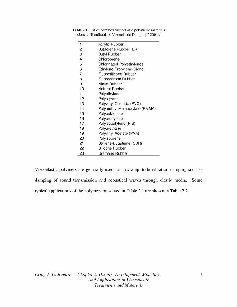
Table 2.1.
Craig A. Gallimore Chapter 2: History, Development, Modeling
And Applications of Viscoelastic
Treatments and Materials
7
Table 2.1 List of common viscoelastic polymeric materials
(Jones, “Handbook of Viscoelastic Damping,” 2001).
1 Acrylic Rubber
2 Butadiene Rubber (BR)
3 Butyl Rubber
4 Chloroprene
5 Chlorinated Polyethylenes
6 Ethylene-Propylene-Diene
7 Fluorosilicone Rubber
8 Fluorocarbon Rubber
9 Nitrile Rubber
10 Natural Rubber
11 Polyethylene
12 Polystyrene
13 Polyvinyl Chloride (PVC)
14 Polymethyl Methacrylate (PMMA)
15 Polybutadiene
16 Polypropylene
17 Polyisobutylene (PIB)
18 Polyurethane
19 Polyvinyl Acetate (PVA)
20 Polyisoprene
21 Styrene-Butadiene (SBR)
22 Silicone Rubber
23 Urethane Rubber
Viscoelastic polymers are generally used for low amplitude vibration damping such as
damping of sound transmission and acoustical waves through elastic media. Some
typical applications of the polymers presented in Table 2.1 are shown in Table 2.2.

Craig A. Gallimore Chapter 2: History, Development, Modeling
And Applications of Viscoelastic
Treatments and Materials
8
Table 2.2. Some common applications for viscoelastic materials
Common Viscoelastic Material Applications
Grommets or Bushings
Component Vibration Isolation
Acoustical Damping of Planar Surfaces
Aircraft Fuselage Panels
Submarine Hull Separators
Mass Storage (Disk Drive) Components
Automobile Tires
Stereo Speakers
Bridge Supports
Caulks and Sealants
Lubricants
Fiber Optic Compounds
Electrical and Plumbing
2.2 Modeling of Viscoelastic Materials
Unlike structural components which exhibit fairly strait-forward dynamic
response, viscoelastic materials are somewhat more difficult to model mathematically.
Because most high load bearing structures tend to implement high strength metal alloys,
which usually have fairly straight-forward stress-strain and strain-displacement
relationships, the dynamics of such structures are simple to formulate and visualize. An
engineer or analyst need only take into account the varying geometries of these structures
and the loads which are applied to them to accurately model the dynamics because the
material properties of the structure and its components are generally well known.
However, difficulty arises when viscoelastic materials are applied to such structures.
This difficulty is mainly due to the strain rate (frequency), temperature, cyclic strain
amplitude, and environmental dependencies between the viscoelastic material properties
and their associated effect on a structure’s dynamics (Jones, 2001, Sun, 1995).

Craig A. Gallimore Chapter 2: History, Development, Modeling
And Applications of Viscoelastic
Treatments and Materials
9
Additionally, many viscoelastic materials and the systems to which they are applied
exhibit nonlinear dynamics over some ranges of the aforementioned dependencies,
further complicating the modeling process (Jones, 2001).
2.2.1 Properties of Viscoelastic Materials
Mycklestad was one of the pioneering scientists into the investigation of complex
modulus behavior of viscoelastic materials (Jones, 2001, Sun, 1995). Viscoelastic
material properties are generally modeled in the complex domain because of the nature of
viscoelasticity. As previously discussed, viscoelastic materials possess both elastic and
viscous properties. The moduli of a typical viscoelastic material are given in equation set
(2.1)
)1('"'
)1('"'
*
*
η
η
iGiGGG
iEiEEE
+=+=
+=+= (2.1)
where the ‘*’ denotes a complex quantity. In equation set (2.1), as in the rest of this
report, E and G are equivalent to the elastic modulus and shear modulus, respectively.
Thus, the moduli of a viscoelastic material have an imaginary part, called the loss
modulus, associated with the material’s viscous behavior, and a real part, called the
storage modulus, associated with the elastic behavior of the material. This imaginary part
of the modulus is also sometimes called the loss factor of the material, and is equal to the
ratio of the loss modulus to the storage modulus. The real part of the modulus also helps
define the stiffness of the material. Furthermore, both the real and imaginary parts of the
modulus are temperature, frequency (strain rate), cyclic strain amplitude, and
environmentally dependent.

Craig A. Gallimore Chapter 2: History, Development, Modeling
And Applications of Viscoelastic
Treatments and Materials
10
2.2.1.1 Temperature Effects on the Complex Modulus
The properties of polymeric materials which are used as damping treatments are
generally much more sensitive to temperature than metals or composites. Thus, their
properties, namely the complex moduli represented by E, G, and the loss factor η , can
change fairly significantly over a relatively small temperature range. There are three
main temperature regions in which a viscoelastic material can effectively operate, namely
the glassy region, transition region, and rubbery region (Jones, 2001, Sun, 1995). Figure
2.2 shows how the loss factor can vary with temperature.
The glassy region is representative of low temperatures where the storage moduli
are generally much higher than for the transition or rubbery regions. This region is
typical for polymers operating below their brittle transition temperature. However, the
range of temperatures which define the glassy region of a polymeric material is highly
dependent on the composition and type of viscoelastic material. Thus, different materials
can have much different temperature values defining their glassy region. Because the
values of the storage moduli are high, this inherently correlates to very low loss factors.
The low loss factors in this region are mainly due to the viscoelastic material being
unable to deform (having high stiffness) to the same magnitude per load as if it were
operating in the transition or rubbery regions where the material would be softer.
On the other material temperature extreme, the rubbery region is representative of
high material temperatures and lower storage moduli. However, though typical values of
storage moduli are smaller, like the glassy region the material loss factors are also
typically very small. This is due to the increasing breakdown of material structure as the
temperature is increased. In this region, the viscoelastic material is easily deformable,
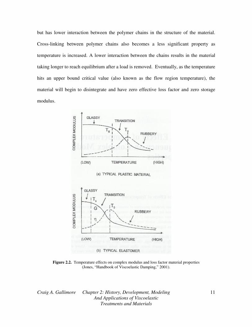
Craig A. Gallimore Chapter 2: History, Development, Modeling
And Applications of Viscoelastic
Treatments and Materials
11
but has lower interaction between the polymer chains in the structure of the material.
Cross-linking between polymer chains also becomes a less significant property as
temperature is increased. A lower interaction between the chains results in the material
taking longer to reach equilibrium after a load is removed. Eventually, as the temperature
hits an upper bound critical value (also known as the flow region temperature), the
material will begin to disintegrate and have zero effective loss factor and zero storage
modulus.
Figure 2.2. Temperature effects on complex modulus and loss factor material properties
(Jones, “Handbook of Viscoelastic Damping,” 2001).

Craig A. Gallimore Chapter 2: History, Development, Modeling
And Applications of Viscoelastic
Treatments and Materials
12
The region falling between the glassy and rubbery regions is known as the
transition region. Materials which are used for practical damping purposes generally
should be used within this region because loss factors rise to a maximum. In more detail,
if a material is within the glassy region and the temperature of the material is increased,
the loss factor will rise to a maximum and the storage modulus will fall to an intermediate
value within the transition region. As the material temperature is further increased into
the rubbery region, the loss factor will begin to fall with the storage modulus. This
behavior is illustrated in Figure 2.2. Therefore, it is extremely important to know the
operating temperature range during the design phase of a host structure to which a
viscoelastic damping treatment will be applied so that the viscoelastic treatment will be
maximally effective.
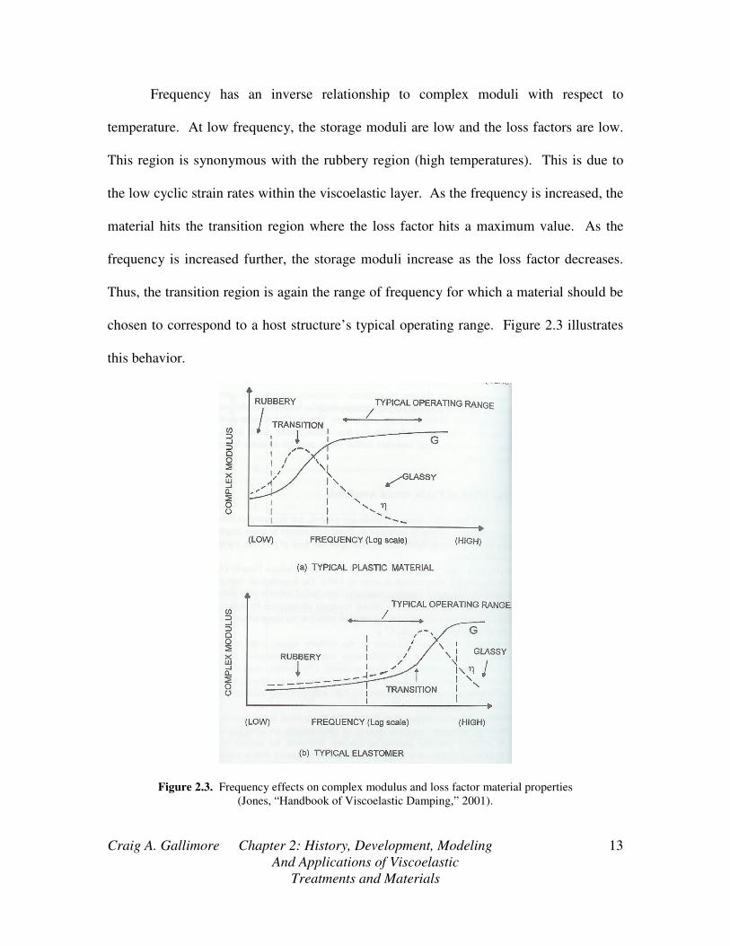
2.2.1.2 Frequency Effects on the Complex Modulus
Like temperature, frequency also has a profound effect on the complex modulus
properties of a viscoelastic polymer, though to a much higher degree with an inverse
relationship. The three regions of temperature dependence (glassy, transition, rubbery)
can sometimes be a few hundred degrees, more than covering a typical operational
temperature range of an engineered structure. But the range of frequency within a
structure can often be several orders of magnitude. The frequency dependence on
complex moduli can be significant from as low as 810− Hz to 810 Hz, a range much too
wide to be measured by any single method (Jones, 2001). Furthermore, relaxation times
after deformation of a viscoelastic material can be anywhere from nanoseconds to years
and will greatly effect one’s measurement methods, especially at low temperatures
(Jones, 2001, Sun, 1995).
Craig A. Gallimore Chapter 2: History, Development, Modeling
And Applications of Viscoelastic
Treatments and Materials
13
Frequency has an inverse relationship to complex moduli with respect to
temperature. At low frequency, the storage moduli are low and the loss factors are low.
This region is synonymous with the rubbery region (high temperatures). This is due to
the low cyclic strain rates within the viscoelastic layer. As the frequency is increased, the
material hits the transition region where the loss factor hits a maximum value. As the
frequency is increased further, the storage moduli increase as the loss factor decreases.
Thus, the transition region is again the range of frequency for which a material should be
chosen to correspond to a host structure’s typical operating range. Figure 2.3 illustrates
this behavior.
Figure 2.3. Frequency effects on complex modulus and loss factor material properties
(Jones, “Handbook of Viscoelastic Damping,” 2001).

Craig A. Gallimore Chapter 2: History, Development, Modeling
And Applications of Viscoelastic
Treatments and Materials
14
2.2.1.3 Cyclic Strain Amplitude Effects on Complex Modulus
The effect of cyclic strain amplitude on polymeric complex moduli is highly
dependent on the composition and type of the polymer, particularly the molecular
structure (Jones, 2001, Sun, 1995). Experiments have shown that the complex moduli of
polymers generally behave linearly only at low cyclic strain amplitudes (Jones, 2001).
There are, however, polymers such as pressure sensitive adhesives, which exhibit
linearity even at high cyclic strain amplitudes. These polymers usually have very few
cross links between long, entangled polymer chains. Therefore, the low interaction
between these chains seems to have an effect on the linear behavior over wide strain
amplitude ranges (Jones, 2001). However, most viscoelastic polymers used in typical
damping applications behave nonlinearly at high strain amplitudes. This nonlinearity is
very difficult to model accurately and involves very complicated theories and a
significant number of tests, many more than for linear complex modulus behavior, to
gather data sufficient to establish trends for a specific material (Jones, 2001, Sun, 1995).
2.2.1.4 Environmental Effects on Complex Modulus
The environment plays a significant role in all outdoor engineering applications.
Temperature ranges, climate, amount of rainfall or direct exposure to sunlight, as well as
foreign substance exposure (such as petroleum products, alkalis, harmful chemicals, etc.)
are necessary design factors to take into consideration for any outdoor engineering
project. The same holds true when considering applying a viscoelastic treatment to an
engineered structure. Temperature dependence on the behavior of viscoelastic complex
moduli has already been discussed. But depending on the application, polymer type, and
composition of the material, exposure to foreign substances must also be addressed. Oils

Craig A. Gallimore Chapter 2: History, Development, Modeling
And Applications of Viscoelastic
Treatments and Materials
15
and other petrols can penetrate into some materials and alter the behavior as well as
jeopardize the bond between a material and the host structure, something which will be
shown to be very important. Therefore, it is important to study the effects of these
foreign elements on the behavior of the material which will be used in a particular
application. Some elements may be more important than others depending on the
operating environment, so these elements should hold the highest interest of the designer.

Craig A. Gallimore Chapter 3: Analytical Mathematical
Models and Viscoelastic Theory
15
Chapter 3
Analytical Mathematical Models and Viscoelastic Theory
There have been several analytical methods developed since the late 1950’s to
predict response of damped systems. Some of the more popular methods include those
developed by Ross, Kerwin, and Ungar (Ross, 1959), Mead and Markus (Mead, 1969),
DiTaranto (DiTaranto, 1965), Yan and Dowell (Yan, 1972), and Rao and Nakra (Rao,
1974). However, the development of finite element software has increased the accuracy
and precision of estimations of the dynamic responses of damped structures. For fairly
simple structures, analytical methods can be used as a substitution for finite element
predictions. Furthermore, finite element packages are often computationally expensive,
something that might not be needed for damping predictions of simpler systems. In this
case, a simple code or program can be written implementing an analytical method to
derive a simple, sufficiently accurate damping model. As the complexity of the system
increases, however, finite element formulations should be strongly considered as the
boundary conditions and system parameters may prove too difficult to define using a
simple analytical based formulation.
3.1 Ross, Kerwin, and Ungar Damping Model
Ross, Kerwin, and Ungar developed one of the earliest damping models for three-
layered sandwich beams based on damping of flexural waves by a constrained
viscoelastic layer. They employed several major assumptions, including (Sun, 1995):
- For the entire composite structure cross section, there is a neutral axis
whose location varies with frequency

Craig A. Gallimore Chapter 3: Analytical Mathematical
Models and Viscoelastic Theory
16
- There is no slipping between the elastic and viscoelastic layers at their
interfaces
- The major part of the damping is due to the shearing of the viscoelastic
material, whose shear modulus is represented by complex quantities in
terms of real shear moduli and loss factors
- The elastic layers displaced laterally the same amount
- The beam is simply supported and vibrating at a natural frequency, or
the beam is infinitely long so that the end effects may be neglected
These assumptions apply to any constrained layer damping treatment applied to a
rectangular beam. Figure 3.1 shows an example system which the Ross, Kerwin, and
Ungar (RKU) equations could be applied to. This laminate beam system is also the lay-
up for the cantilever beam used for materials testing later in this report.
Figure 3.1. Three layer cantilever beam with host beam, viscoelastic layer, and constraining layer clearly
defined.

Craig A. Gallimore Chapter 3: Analytical Mathematical
Models and Viscoelastic Theory
17
Comparison between experimental data and this theory have shown that results from
theory correlate well to experiment (Ross, 1959). The model is represented by a complex
flexural rigidity, (EI)*, where the ‘*’ denotes a complex quantity, given by
+
−
−+
−−
−+−+
++
−−++=
)1(
)()(
2
)(
)()(
)1(
)(12
121212)*(
*
*
22*
2
*
2
33*3
v
ccvsvv
ccvsvv
ss
v
cv
ccvvss
g
DdDdhE
DhhE
DdhEDhhE
DhEg
DdhE
hEhEhEEI
(3.1)
where D is the distance from the neutral axis of the three layer system to the neutral axis
of the host beam,
2
2
)(2
)()2
(
2
1
*
*
***
***
csv
vcc
vv
vsvs
ccsvssvvv
ss
ccvsvvvvsvv
hhhd
phhE
Gg
hhh
hEhEhEghE
hE
dhEhhEgd
hhE
D
++=
=
+=
++++
++−=
(3.2)
In these equations sE , *
vE , cE and sh , vh , ch are the elastic moduli and thicknesses of the
host structure, viscoelastic layer, and constraining layer, respectively. The term *
vg is
known as the ‘shear parameter’ which varies from very low when *
vG is small to a large
number when *
vG is large. The term ‘p’ within the shear parameter is the wave number,
namely the thn eigenvalue divided by the beam length. The shear parameter can also be
expressed in terms of modal frequencies by

Craig A. Gallimore Chapter 3: Analytical Mathematical
Models and Viscoelastic Theory
18
ss
nssn
nncvc
vv
IE
Lbh
ChhE
LGg
424
2
2**
ωρξ
ξ
=
=
(3.3)
where nω is the thn modal frequency and nC are correction factors determined by Rao
(Rao, 1974) and are given in Table 3.1.
Table 3.1. Rao correction factors for shear parameter in RKU equations
(Jones, “Handbook of Viscoelastic Damping,” 2001).
Boundary Conditions Correction Factor
Mode 1 Mode 2+
Pinned-Pinned 1 1
Clamped-Clamped 1.4 1
Clamped-Pinned 1 1
Clamped-Free 0.9 1
Free-Free 1 1
Additionally, a more detailed analysis using the Ross, Kerwin, Ungar (RKU)
equations will be presented in the analysis portion of this document allowing for
correction factors. This system of equations will be the main method of analysis used in
the remainder of this report.
3.2 Beam Theory Methods of Analysis
Several other methods of analysis have been developed by authors like Mead and
Markus, DiTaranto, Yan and Dowell, and Rao and Nakra, all of which rely on either
Euler-Bernoulli beam theory or principles such as virtual work, often resulting in sixth-
order linear homogenous differential equations. Though these analyses are useful in
many applications, they are often specific or most easily applied to a special type of
boundary condition or loading function. Kalyanasundaram (Kalyanasundaram, 1987)

Craig A. Gallimore Chapter 3: Analytical Mathematical
Models and Viscoelastic Theory
19
and Buhariwala (Buhariwala, 1988) also developed and used beam theory models of
viscoelastic structures. Kalyanasundaram analyzed and predicted dynamics of
viscoelastic structures using the Timoshenko beam method. Buhariwala used
d’Alembert’s principle and the principle of virtual work to predict dynamics of
viscoelastically damped structures. It will be shown that the RKU equations, when used
with other vibration analysis tools, are easier to manipulate and provide very simple,
sufficiently accurate predictions of structural damping.
3.3 Rayleigh Quotient Analysis
In undamped vibration theory, the Rayleigh Quotient is a useful method for
estimation of modal frequencies of a system. The Rayleigh Quotient for an undamped
system is given by
REF
MAX
L
r
L
r
rrT
V
dxxYxm
dxdx
xYdEI
dx
dxY
xYR =
==
∫
∫
0
2
0
2
2
2
2
2
)()(
)()(
)]([ ω (3.4)
where )(xYr is an approximated mode shape, ω is a modal frequency, MAXV is the
maximum potential (strain) energy, and REFT is a reference kinetic energy. A complex
version of the Rayleigh Quotient was developed by Torvik (Torvik, 1996), where he used
complex approximations of the mode shapes. The resulting Complex Rayleigh Quotient
is derived from the equations of motion and given by
dxuu
dxuu
uu
T
L
T
L
0
_
0
_
2
2
M
L
LM
∫
∫=Ω
=Ω
(3.5)

Craig A. Gallimore Chapter 3: Analytical Mathematical
Models and Viscoelastic Theory
20
where M and L are complex matrix symmetric linear operators which include spatial
derivatives. The terms in these matrices depend on the derivation of the equations of
motion of the system. The second equation in (3.5) is the complex Raleigh Quotient.
The u terms are vectors containing complex mode shapes. If real quantities are used in
the Complex Rayleigh Quotient (CRQ), the equation reduces to modal strain energy, or
the real form of the Rayleigh Quotient.
3.4 Fractional Calculus Analysis
Fractional calculus and the fractional derivative were developed by Liouville in a
paper from 1832. Fractional calculus is a branch of mathematics which studies the
possibility of taking real number powers of differential operators. This concept can also
be applied to viscoelastic analysis as used by Bagley and Torvik (Bagley, 1985). It is
also the primary method of analysis used by Jones, and Nashif and Henderson (Nashif,
1985). The foundation of the fractional calculus model is found in accepted molecular
theories governing mechanical behavior of viscoelastic media (Bagley, 1985). The
analysis of structural responses can be calculated for any loading having a Laplace
transform. Thus, the responses are always real, continuous, and causal functions of time
(Bagley, 1985, Jones, 2001). When compared to other current methods, the fractional
calculus model has two significant advantages. First, there are not a large number of
derivative terms as with the method of trying to relate time dependent stresses and strains
through time derivatives acting on stress and strain fields. Second, a complex frequency
dependent modulus, as in the Rayleigh quotient method, often does not satisfy specific
mathematical relationships between the real and imaginary parts of the modulus.

Craig A. Gallimore Chapter 3: Analytical Mathematical
Models and Viscoelastic Theory
21
3.5 Partial Viscoelastic Treatments
Damping treatments can also be applied in a partial manner, namely, to specific
points in a structure rather than the entire structure. An analysis of partially damped
structures was developed by Moreira et al. (Moreira, 2006). Partial constrained layer
damping treatments have two significant advantages, they lower additional mass and
stiffness, and more importantly can be just as effective at damping as a complete
treatment if the correct application areas are targeted. Moreira found that if the
viscoelastic layer is located near a neutral plane of the structure (i.e. sandwich type
structures) the layer must be placed on nodal areas where shear deformation reaches a
maximum on the neutral axis. Alternatively, if the viscoelastic layer is located far from
the neutral plane (i.e surface treatments), more deformation is expected on anti-nodal
areas since flexural deformation of the host structure reaches a maximum (Moreira,
2006). Intuitively, this makes sense because the primary mechanism of viscoelastic
damping is shear. Thus, if damping material is applied to host structure areas having the
highest surface strains, the partial treatment will utilize the areas of the structure having
the majority of the strain energy within the structure, resulting in maximized damping for
a partial treatment. Moreira’s method utilizes an energy balance between the strain
energy of the entire structure and the strain energy of the treated area. This ratio is
deemed the Modal Strain Energy Ratio, given by
r
T
r
rc
T
r
K
KMSER
][
][
φφ
φφ= (3.6)
Where rφ is the thr modal shape vector, [K] is the finite element stiffness matrix for the
host structure, and ][ cK is the stiffness matrix of the structure with applied viscoelastic
Craig A. Gallimore Chapter 3: Analytical Mathematical
Models and Viscoelastic Theory
22
treatment. This ratio should, in general, be maximized so that the modal strain energy of
the covered area is as close to the modal strain energy of the entire structure. However,
this is somewhat difficult because the coverage areas depend on the mode of vibration.
Therefore, it is difficult to design an effective partial viscoelastic treatment for a
broadband application. Though this analysis seems fairly straight-forward, deriving the
stiffness matrices in the Modal Strain Energy Ratio is complex for more complicated
structures and is best solved using finite element software.
Craig A. Gallimore Chapter 4: Damping Considerations for
Landing Gear Applications
23
Chapter 4
Damping Considerations for Landing Gear Applications
The design of landing gear with respect to structural damping using viscoelastic
materials poses a unique kind of problem. Traditional landing gear often implement
shock absorbers and dashpots. However, these components can be bulky and heavy,
affecting the aerodynamic efficiency and flight time of aircraft. Additionally, there are
usually a host of customer requirements specific to the project and application which
generally govern the scope and intensity of the design phase of the landing gear. With
these factors in mind, the role of a damping treatment can be discussed in more detail.
4.1 Impact of Aerodynamics and Weight on Damping Treatment
Aerodynamics and weight are two significant concerns when designing landing
gear. The gear of any aircraft should be streamlined and optimized so that the gear is not
only as lightweight as possible, but also has a minimal frontal profile to minimize drag
during flight. Lightweight materials should be chosen when possible so that the weight
addition of the gear to the aircraft is at a minimum, effectively increasing the maximum
flight time of the aircraft.
In this particular application, the damping treatment should be as thin and
lightweight as possible, while still contributing a large amount of damping to the gear.
This significantly narrows the field of damping materials which should be used,
effectively eliminating high density polymers, though their damping may be quite
significant over the small range of effective vibration modes a landing gear will
experience during landing. Additionally, this implies that a viscoelastic polymer should

Craig A. Gallimore Chapter 4: Damping Considerations for
Landing Gear Applications
24
be chosen which has the highest loss factors and lowest shear modulus available at lower
vibration modes, further narrowing the available selection of materials. Additionally,
viscoelastic materials generally have better damping at higher modes because the strain
rates, which depend on modal frequencies, are higher. The configuration of the
viscoelastic material will be dependent on the geometry of the host structure. The host
structure needs to be properly designed so that it not only has a minimal frontal profile,
but that its profile is minimally affected by the addition of a damping treatment.
4.2 Landing Environment on Damping Considerations
The damping treatment for the landing gear discussed in this report is to be
applied to a 400 pound fixed wing unmanned aerial vehicle which operates in all forms of
weather conditions, including rain, sleet, snow, sand, foreign chemicals, direct heat or
sunlight. Additionally, because the vehicle is unmanned, there are no pilot corrections
for terrain or surface variability. The aircraft could land on grass, concrete, asphalt,
packed dirt, or even snow or ice, each having different friction and coefficients of
restitution.
Many different viscoelastic polymers have various resistances to the elements. As
previously mentioned in section 2.1, viscoelastic polymers and their properties can be
engineered and manufactured for a multitude of specific applications. Fortunately, the
same is true for environmental resistance. Many viscoelastic polymers are designed
specifically for outdoor environments and are resistant to harsh chemicals like alkalis or
mild acids, moisture, oils and solvents, and some are even flame retardant.
An unmanned aerial vehicle is often subject to vehicle dynamics on the extreme
boundaries of its design envelope. The UAV must calculate and act on flight speed,

Craig A. Gallimore Chapter 4: Damping Considerations for
Landing Gear Applications
25
approach angle, wind conditions, and flap adjustments in some of the most adverse
environmental conditions. This often results in the aircraft having a ‘heavy’ landing
causing a higher than normal impact load on the landing gear and fuselage. Thus, a
viscoelastic treatment should be designed in such a way as to account for factors of safety
and extreme landings. The treatment should be sparse enough as to not significantly
increase the weight and aerodynamic drag of the aircraft, but also robust enough to
handle the most extreme vibration a landing gear will see in the most extreme operating
conditions.

Craig A. Gallimore Chapter 5: Instrumentation and Data
Acquisition
26
Chapter 5
Instrumentation and Data Acquisition
There are two testing and data acquisition systems used in this research project.
The first is a cantilever beam system for characterization of various damping materials
used as prospective solutions for damping a cantilever type spring design for aircraft
landing gear. The second is a cyclic loading machine used to extract the viscoelastic
properties, namely the complex moduli, of various materials.
The data acquisition system for the damping characterization rig is presented in
figures 5.1a and 5.1b. Figure 5.1a shows the general flow of information through the
data acquisition system (DAQ) while Figure 5.1b shows the actual components of the
DAQ.
Figure5.1a. Shows the flow of information from the transducers the signal express software.

Craig A. Gallimore Chapter 5: Instrumentation and Data
Acquisition
27
b)
Figure 5.1b. Shows the DAQ in its entirety with all components.
The transducers used were PCB (Piezoelectronics) model 3801D1FB206/M001 single
axis accelerometers shown in Figure 5.2.
Figure 5.2. Photograph of accelerometers used in cantilever beam testing.
Craig A. Gallimore Chapter 5: Instrumentation and Data
Acquisition
28
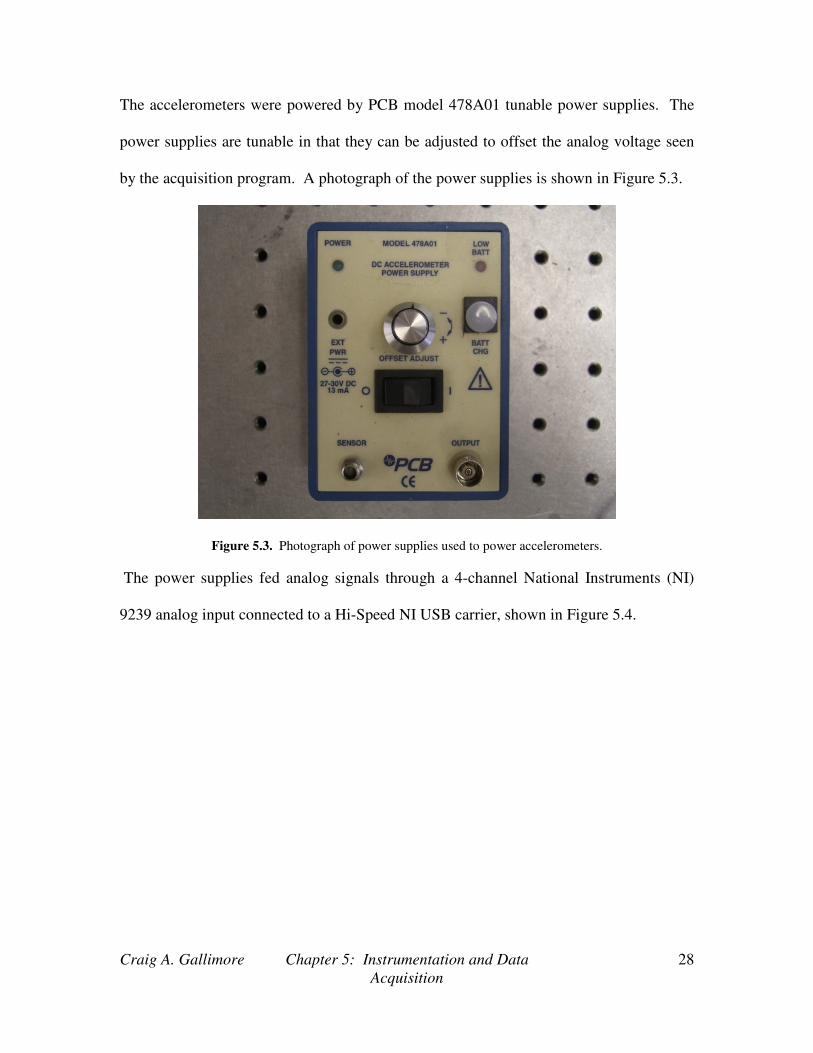
The accelerometers were powered by PCB model 478A01 tunable power supplies. The
power supplies are tunable in that they can be adjusted to offset the analog voltage seen
by the acquisition program. A photograph of the power supplies is shown in Figure 5.3.
Figure 5.3. Photograph of power supplies used to power accelerometers.
The power supplies fed analog signals through a 4-channel National Instruments (NI)
9239 analog input connected to a Hi-Speed NI USB carrier, shown in Figure 5.4.

Craig A. Gallimore Chapter 5: Instrumentation and Data
Acquisition
29
Figure 5.4. Four channel analog input and NI USB carrier.
Finally, LabVIEW’s Signal Express 8.0 was used to collect and analyze data from the
accelerometers. Signal Express was configured to collect 6000 samples at 1000 Hz for
data analysis.
Viscoelastic material samples were tested using an ElectroPuls E1000 cyclic
loading machine shown in figure 5.5a and 5.5b. Each specimen was loaded into the grips
of the machine (Figure 5.5b) and cyclically loaded in tension and/or compression to
generate stress-strain plots of the loading history of each viscoelastic material. The
ElectroPuls machine is capable of controlling the strain rate and strain amplitude of each
test, with an upper frequency limit of 300 Hz. Stress-strain behavior and the extraction of
viscoelastic material properties from tests conducted with the ElectroPuls machine are
explained in Chapter 6.

Craig A. Gallimore Chapter 5: Instrumentation and Data
Acquisition
30
a) b)
Figure 5.5. a) Photograph of ElectroPuls E1000 cyclic loading machine. b) Photograph of ElectroPuls
E1000 grips with sample viscoelastic specimen loaded for testing.
Craig A. Gallimore Chapter 6: Experimental Determination
Of Viscoelastic Material Properties
31
Chapter 6
Experimental Determination of Viscoelastic Material
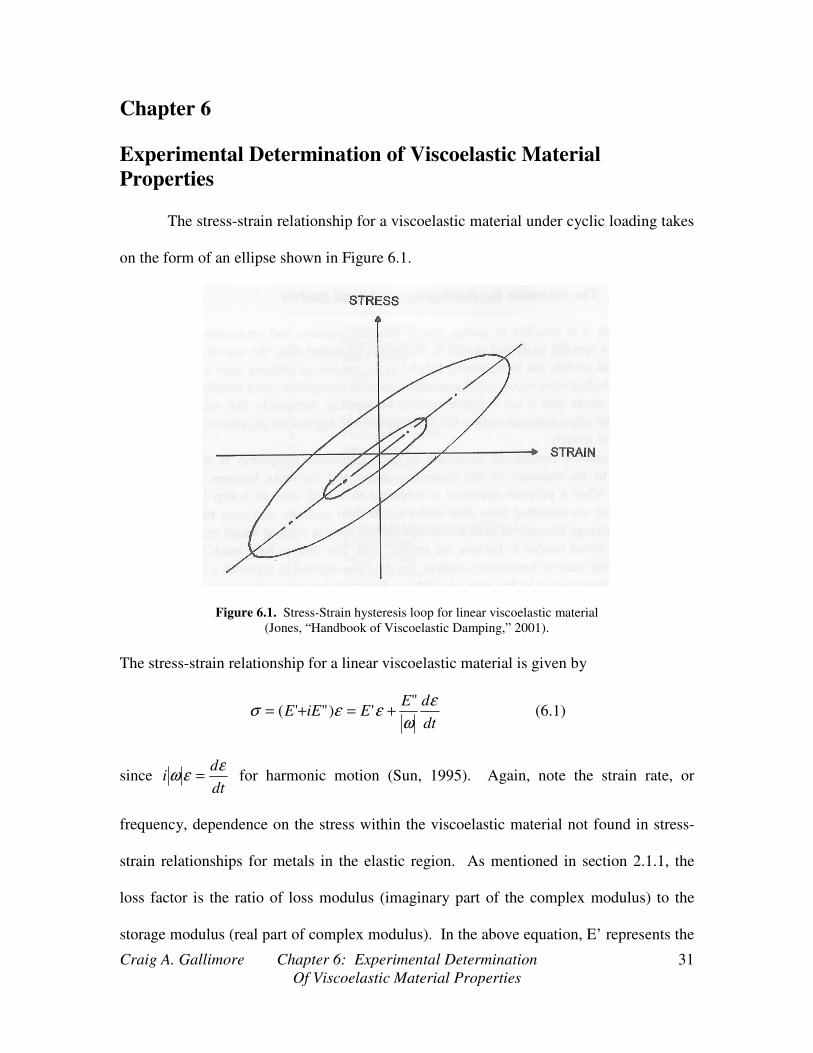
Properties The stress-strain relationship for a viscoelastic material under cyclic loading takes
on the form of an ellipse shown in Figure 6.1.
Figure 6.1. Stress-Strain hysteresis loop for linear viscoelastic material
(Jones, “Handbook of Viscoelastic Damping,” 2001).
The stress-strain relationship for a linear viscoelastic material is given by
dt
dEEiEE
ε
ωεεσ
"')"'( +=+= (6.1)
since dt
di
εεω = for harmonic motion (Sun, 1995). Again, note the strain rate, or
frequency, dependence on the stress within the viscoelastic material not found in stress-
strain relationships for metals in the elastic region. As mentioned in section 2.1.1, the
loss factor is the ratio of loss modulus (imaginary part of the complex modulus) to the
storage modulus (real part of complex modulus). In the above equation, E’ represents the

Craig A. Gallimore Chapter 6: Experimental Determination
Of Viscoelastic Material Properties
32
storage modulus, synonymous with the elastic modulus for metals. Sun and Lu explain
that the area enclosed by the ellipse in Figure 6.1 is equal to the energy dissipated by the
viscoelastic material per loading cycle. Additionally, the slope of the major axis of the
ellipse in Figure 6.1 is representative of the storage modulus of the viscoelastic material.
Thus, E’ is easily found from the hysteresis plot of stress and strain.
From Figure 6.1, it should be noted that the general shape of the ellipse does not
change for small variations of the maximum strain amplitude, 0ε . However, the shape
does change as the loss factor changes (i.e. the inner ellipse and outer ellipse in Figure
6.1 are tests at the same frequency but different strain amplitudes). Thus, the ratio of the
minor axis to major axis of the ellipse can be used as a measure of damping (Jones,
2001). However, this ratio is not the loss factor of the material. To find the loss factor of
the material, the data generated using the ElectroPuls E1000 can be used to find the
energy dissipated per cycle of loading for each viscoelastic material. The energy
dissipated is given by the path integral
2
0
/2
0
"επε
σεσωπ
Edtdt
ddWd === ∫ ∫ (6.2)
It is also important to find the peak potential energy within the material during a loading
cycle. Peak potential energy is given by
2
0'2
1εEU = (6.3)
From the energy dissipated per cycle and the peak potential energy the loss factor can be
found to be
'
"
2 E
E
U
Wd ==π
η (6.4)

Craig A. Gallimore Chapter 6: Experimental Determination
Of Viscoelastic Material Properties
33
Another method of measuring the properties of viscoelastic materials was formulated by
Lemerle (Lemerle, 2002), but the analysis used by Sun and Lu is accurate and relatively
simple by comparison.
6.1 Viscoelastic Materials Testing
The design of this landing gear system, as in many other engineering projects, is
heavily dependent on customer requirements. Weight, aerodynamics, cost, and most
significantly reliability and operability are all serious concerns which must be accounted
for during the design phase. Cost, reliability, and predictability, in particular, are the
main foci of this section. Eight different damping materials where chosen and tested,
each having different material properties and durometers. Seven of these materials were
chosen because they are common rubbers, available at almost any polymer distributer.
Additionally, because they are common, they are often the cheapest because they are
manufactured in the highest quantities. These common rubbers have little to no damping
property documentation and are generally used for simple vibration isolation
applications. After testing, all materials were found to be sufficiently predictable in their
dynamics, and all are very reliable because of their high durability.
The materials chosen for testing were various grades of butyl, nitrile, vinyl,
silicon, and SBR rubbers. Table 6.1 lists all materials tested as well as a summary of
their known preliminary properties before testing.
Craig A. Gallimore Chapter 6: Experimental Determination
Of Viscoelastic Material Properties
34
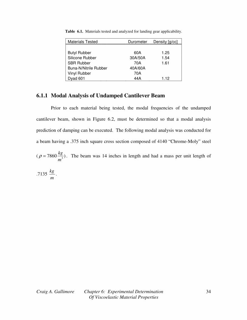
Table 6.1. Materials tested and analyzed for landing gear applicability.
Materials Tested Durometer Density [g/cc]
Butyl Rubber 60A 1.25
Silicone Rubber 30A/50A 1.54
SBR Rubber 70A 1.61
Buna-N/Nitrile Rubber 40A/60A
Vinyl Rubber 70A
Dyad 601 44A 1.12
6.1.1 Modal Analysis of Undamped Cantilever Beam
Prior to each material being tested, the modal frequencies of the undamped
cantilever beam, shown in Figure 6.2, must be determined so that a modal analysis
prediction of damping can be executed. The following modal analysis was conducted for
a beam having a .375 inch square cross section composed of 4140 “Chrome-Moly” steel
( )78603
m
kg=ρ . The beam was 14 inches in length and had a mass per unit length of
.7135 m
kg.

Craig A. Gallimore Chapter 6: Experimental Determination
Of Viscoelastic Material Properties
35
Figure 6.2. Undamped cantilever beam used for damping material characterization.
In this order, once the modal frequencies are known, the materials can be tested at these
frequencies, their properties (Moduli and loss factors) determined, and thicknesses of
damping layers found using a MATLAB program (see appendix A) to predict effective
damping at each mode. Lastly, actual tests can be carried out using the thicknesses
predicted from MATLAB to find a correlation between theoretical and experimental
results.
To find the modal frequencies of an undamped cantilever beam with a tip mass,
simple modal analysis can be used. By using a cantilever beam mode shape (Meirovitch,
2001),
xDxCxBxAxY rrrrrrrrr ββββ coshsinhcossin)( +++= (6.5)
Craig A. Gallimore Chapter 6: Experimental Determination
Of Viscoelastic Material Properties
36
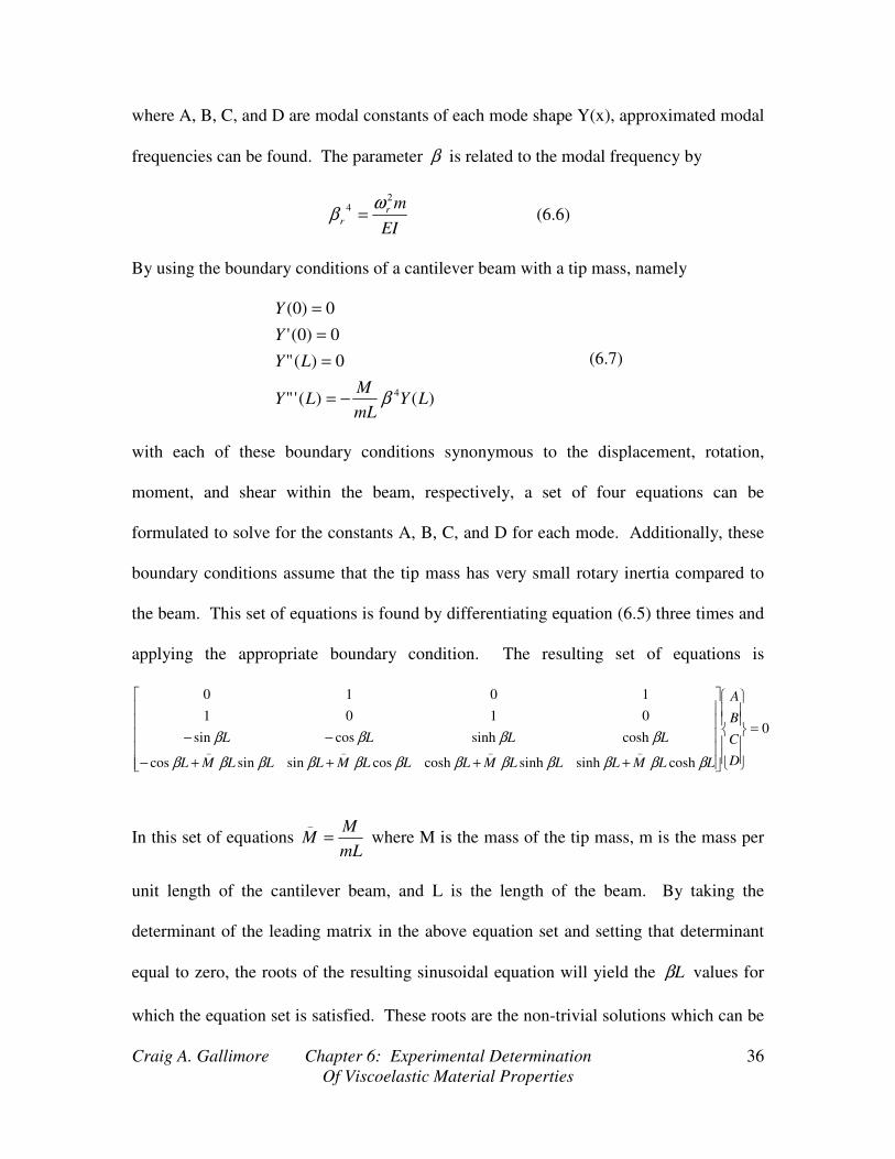
where A, B, C, and D are modal constants of each mode shape Y(x), approximated modal
frequencies can be found. The parameter β is related to the modal frequency by
EI
mr
r
24 ω
β = (6.6)
By using the boundary conditions of a cantilever beam with a tip mass, namely
)()('"
0)("
0)0('
0)0(
4LY
mL
MLY
LY
Y
Y
β−=
=
=
=
(6.7)
with each of these boundary conditions synonymous to the displacement, rotation,
moment, and shear within the beam, respectively, a set of four equations can be
formulated to solve for the constants A, B, C, and D for each mode. Additionally, these
boundary conditions assume that the tip mass has very small rotary inertia compared to
the beam. This set of equations is found by differentiating equation (6.5) three times and
applying the appropriate boundary condition. The resulting set of equations is
0
coshsinhsinhcoshcossinsincos
coshsinhcossin
0101
1010
____
=
++++−
−−
D
C
B
A
LLMLLLMLLLMLLLML
LLLL
ββββββββββββ
ββββ
In this set of equations mL
MM =
_
where M is the mass of the tip mass, m is the mass per
unit length of the cantilever beam, and L is the length of the beam. By taking the
determinant of the leading matrix in the above equation set and setting that determinant
equal to zero, the roots of the resulting sinusoidal equation will yield the Lβ values for
which the equation set is satisfied. These roots are the non-trivial solutions which can be

Craig A. Gallimore Chapter 6: Experimental Determination
Of Viscoelastic Material Properties
37
used to find the modal frequencies of the cantilever beam shown in Figure 6.2. If _
M =1,
that is the mass at the tip is equal to the mass of the beam, the resulting modal
frequencies are presented in Table 6.2 for the first five modes.
Table 6.2. Modal frequencies of first five modes for cantilever beam with tip mass M=mL.
Mode Beta_L Modal Frequency
(rad/s) Modal Frequency
(Hz)
1 1.248 177.128 28.19082057
2 4.0312 1848.111 294.1362495
3 7.1341 5783.74 920.5115881
4 10.2566 11883.378 1891.299947
5 13.3878 20383.47 3244.132748

Craig A. Gallimore Chapter 7: Testing of Materials
Using ElectroPuls E1000 Cyclic
Loading Machine
38
Chapter 7
Testing of Materials Using ElectroPuls E1000 Cyclic Loading
Machine
A total of seven materials were tested in the ElectroPuls E1000 cyclic loading
machine at frequencies of 1, 5, 10, 15 and 28.19 Hz. The first four frequencies, namely
1, 5, 10, and 15 Hz, where selected for testing to establish trends and ensure that the data
for the first modal frequency was accurate. From the modal frequencies listed in Table
6.2, 28.19 Hz corresponds to the first modal frequency of the cantilever beam analyzed in
section 6.1.1. However, the ElectroPuls has a maximum loading frequency of 100 Hz
where sufficient strains within the sample can be measured accurately. Thus, only the
data for the first modal frequency of each material sample will be analyzed in the
following sections. This is sufficient, because when applied to the aircraft landing gear,
the most obvious, and therefore more prominent, dynamics will occur at lower frequency,
much lower than 294 Hz at the second mode. It is also reasonable to say that so long as
the material is not operating within the glassy region of frequency and temperature,
damping of vibrations at the second mode and above will be much greater than damping
at the first mode. Thus, the damping values presented for the first modes of vibration in
the materials will generally be lower than the subsequent modes, making the damping of
first mode vibrations the driving factor in the design of the gear.
The storage modulus, shear modulus, and loss factor were determined for each
material at each frequency. The method of analysis was generalized in section 6.0, and
will be extended to the method of parameter determination for each material in the
following sections. One of the seven materials exhibited nonlinear viscoelastic behavior,

Craig A. Gallimore Chapter 7: Testing of Materials
Using ElectroPuls E1000 Cyclic
Loading Machine
39
so variations or approximations in the method in section 6.0 were made to approximate
material properties. Additionally, for the cyclic loading tests at 28.19 Hz, the primary
frequency of interest, the materials were assumed to behave as linearly viscoelastic
materials, so the analysis used in section 6.0 sufficiently describes the relationship
between the stress and strain of the viscoelastic material.
7.1 Analysis Methodology and Testing Assumptions
Each test sample was loaded into the ElectroPuls machine with a configuration
shown in Figure 5.6b. Upon testing the sample at different frequencies, Microsoft Excel
was used to analyze the data taken by the transducers within the ElectroPuls. The
generated data consisted of time, load, and position. The position is in reference to the
position of the grips used to secure the test article during data sampling. The load and
position measured by the ElectroPuls were then converted to engineering stress and strain
within Microsoft Excel. For this conversion, several major assumptions had to be made:
1. The stress is uniform throughout the cross section of the material and the
approximation that stress is equal to the load divided by the original cross
sectional area hold
2. The strain is uniform throughout the length of the specimen and is equal to the
change in position of the grips divided by the original length of the specimen.
Neither of these approximations is entirely accurate for reasons which will be discussed.
However, for the purposes of this report, they are sufficient to provide accurate relative
results. The purpose of this testing is not to produce and publish exact material data for
each material. This would have been possible if strain gauges or extensometers were
available to accurately measure the strain within the sample. However, it is the purpose

Craig A. Gallimore Chapter 7: Testing of Materials
Using ElectroPuls E1000 Cyclic
Loading Machine
40
of this testing to provide a relative comparison of several damping materials. Though the
material data may not be exactly accurate due to the assumptions made above, each
material was tested and analyzed using the same methods and assumptions. It inherently
follows that each material can be compared with all other materials because they all fall
under the same assumptions and experimental error. Thus, the best damping materials
within the set of those tested can be established, though the data may not be as accurate if
more precise testing methods could have been used.
The assumptions stated above are not entirely accurate for several reasons. The
first is that the material is being held in place by grips which produce a lateral stress at
locations near the grips. Thus, the material can no longer be assumed to be in a perfect
state of uniaxial stress. However, at locations far from the grips (center of the test
specimen), the assumptions are reasonably accurate. The second reason is that no
material is completely homogeneous or isotropic, particularly polymers. There are
always variations in the structure of a material sample no matter how precise the
manufacturing methods. Unlike metals, polymers do not have predictable patterns of
microstructure. Rather, they are a mixture of long entangled chains of random order and
length. For the purposes of this report, it is assumed that each material is homogeneous
and isotropic, so only two material properties are needed to describe a state of stress and
strain. These material properties are the elastic or storage modulus, and Poisson’s ratio,
which for most of the test materials is assumed to be very close to .5. Because the
materials are assumed homogeneous and isotropic, once the elastic modulus, or storage
modulus, is known from the tests, the shear modulus can be found from

Craig A. Gallimore Chapter 7: Testing of Materials
Using ElectroPuls E1000 Cyclic
Loading Machine
41
)1(2
''
υ+=
EG (7.1)
This equation should be found in any undergraduate mechanics of materials textbook.
As a further disclaimer, it should be noted that in no way does the data presented
in the following sections exactly match the material properties of each material. Rather,
the data presented in the following sections is to establish relative trends and approximate
numbers so that the best damping material to apply to an aircraft landing gear, the
ultimate goal of this report, can be identified.
7.1.1 Extracting Data using Microsoft Excel
As mentioned in section 7.1, during each test, data was recorded to Microsoft
Excel for analysis. After the conversion of load and position to stress and strain,
respectively, analyses had to be carried out to find the work done per cycle, the storage
modulus, maximum strain amplitude, and loss factor using the theory presented in section
6.0. However, direct integration to find the work done by the viscoelastic material, or
energy dissipated as heat, per cycle is impossible because of the nature of the data taken.
In order to find the energy dissipated per cycle, equation (6.2) in section 6.0 is equivalent
to
∫ ∑ ∑= =
+++ −−=∆−==N
i
N
i
iiiiiiid dW1 1
111 ))(()( εεσσεσσεσ (7.2)
where N is the number of samples taken and 1σ is a static pre-stress on the material.
The storage modulus of the material at a given frequency (independent of strain
amplitude) is found by examining an engineering stress vs. strain plot. The storage
modulus is the linear trend of the data, shown in Figure 7.1, given by a trend line. The

Craig A. Gallimore Chapter 7: Testing of Materials
Using ElectroPuls E1000 Cyclic
Loading Machine
42
storage modulus is equivalent to the slope of the major axis of the ellipse generated by
the loading of the material.
SBR 70A Stress vs. Strain - 5mm,5Hz
y = 8.1663x - 0.0283
-0.1
0
0.1
0.2
0.3
0.4
0.5
0.6
-0.01 0 0.01 0.02 0.03 0.04 0.05 0.06 0.07
Strain
Str
ess [
MP
a]
SBR 70A - 5Hz
Linear (SBR 70A - 5Hz)
Figure 7.1. Example plot of stress and strain for SBR 70A Rubber. Trend line slope gives storage
modulus.
Sample loading curves for a material at two different frequencies are shown in Figures
7.2a and 7.2b. Additionally, the corresponding stress vs. strain curves for Figures 7.2a
and 7.2b are shown in Figures 7.3a and 7.3b, respectively. This illustrates how the shape,
and inherently area, of the ellipses change with varying frequency. As the ratio of the
minor to major axes of the ellipse changes with frequency, so does the loss factor.
However, a change in strain amplitude does not have an impact on the damping factor of
a material so long as the frequency is held constant.

Craig A. Gallimore Chapter 7: Testing of Materials
Using ElectroPuls E1000 Cyclic
Loading Machine
43
Loading curve for SBR 70A Rubber
-1.00E-02
0.00E+00
1.00E-02
2.00E-02
3.00E-02
4.00E-02
5.00E-02
6.00E-02
0 0.5 1 1.5 2 2.5 3 3.5 4
Time [s]
Lo
ad
[k
N]
SBR 70A Loading - 5Hz
Loading Curve for SBR Rubber 70A - 15Hz
-1.00E-02
0.00E+00
1.00E-02
2.00E-02
3.00E-02
4.00E-02
5.00E-02
6.00E-02
0 1000 2000 3000 4000 5000 6000
Time [s]
Lo
ad
[k
N]
SBR 70A Loading - 15 Hz
a) b)
Figure 7.2. a) Load versus time plot at low frequency. b) Load versus time plot at high frequency
SBR 70A Stress vs. Strain - 5mm,5Hz
y = 8.1663x - 0.0283
-0.1
0
0.1
0.2
0.3
0.4
0.5
0.6
-0.01 0 0.01 0.02 0.03 0.04 0.05 0.06 0.07
Strain
Str
ess [
MP
a]
SBR 70A - 5Hz
Linear (SBR 70A - 5Hz)
SBR 70A Stress vs. Strain - 5mm,15Hz
y = 8.8745x - 0.02
-0.1
0
0.1
0.2
0.3
0.4
0.5
0 0.01 0.02 0.03 0.04 0.05 0.06
Strain
Str
es
s [
MP
a]
SBR 70A - 15 Hz
Linear (SBR 70A - 15 Hz)
a) b)
Figure 7.3. a) Stress versus strain plot for Figure 7.2a. b) Stress versus strain plot for Figure 7.2b.
7.2 Butyl 60A Rubber Testing
Butyl rubber is a synthetic rubber produced by polymerization of about 98%
isobutylene with about 2% of isoprene. Butyl rubber is also known as polyisobutylene or
PIB. It has excellent impermeability and its long polymer chains give it excellent flex
properties. Butyl is often used in making adhesives, agricultural chemicals, fiber optic
compounds, caulks and sealants, cling films, electrical fluids, lubricants such as 2 cycle
engine oil, as a gasoline/diesel fuel additive, and even chewing gum. The first major
application of butyl was tire inner tubes because of its excellent impermeability to air. It
was chosen for testing because it is very common and extremely cheap, while still
providing excellent flexural and damping properties.
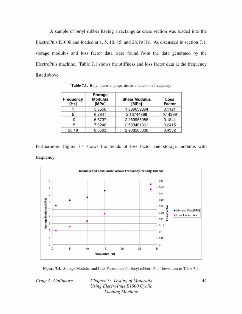
Craig A. Gallimore Chapter 7: Testing of Materials
Using ElectroPuls E1000 Cyclic
Loading Machine
44
A sample of butyl rubber having a rectangular cross section was loaded into the
ElectroPuls E1000 and loaded at 1, 5, 10, 15, and 28.19 Hz. As discussed in section 7.1,
storage modulus and loss factor data were found from the data generated by the
ElectroPuls machine. Table 7.1 shows the stiffness and loss factor data at the frequency
listed above.
Table 7.1. Butyl material properties as a function a frequency.
Frequency [Hz]
Storage Modulus
[MPa] Shear Modulus
[MPa] Loss
Factor
1 5.5556 1.889659864 0.1121
5 6.2841 2.13744898 0.14299
10 6.6737 2.269965986 0.1841
15 7.6246 2.593401361 0.2415
28.19 8.5503 2.908265306 0.4332
Furthermore, Figure 7.4 shows the trends of loss factor and storage modulus with
frequency.
Modulus and Loss factor versus Frequency for Butyl Rubber
0
1
2
3
4
5
6
7
8
9
0 5 10 15 20 25 30
Frequency [Hz]
Sto
rag
e M
od
ulu
s [
MP
a]
0
0.05
0.1
0.15
0.2
0.25
0.3
0.35
0.4
0.45
0.5
Lo
ss F
acto
r
Modulus Data [MPa]
Loss Factor Data
Figure 7.4. Storage Modulus and Loss Factor data for butyl rubber. Plot shows data in Table 7.1.

Craig A. Gallimore Chapter 7: Testing of Materials
Using ElectroPuls E1000 Cyclic
Loading Machine
45
It is seen from Figure 7.4 that both the storage modulus and loss factor increase with
increasing frequency. Over this relatively small frequency range, the loss factor almost
quadruples its value as the frequency is increased from 1 Hz to 28.19 Hz. The storage
modulus of the sample also sees fairly significant increases from 5.55 MPa to 8.55 MPa,
about 1.5 times the original value at 1 Hz. Based on the low frequency and moderate
temperature (the materials were tested at room temperature of about 70 degrees), the
material is most likely operating in its rubbery region. Butyl rubber typically has a
service temperature range of about -13 – 248 degrees Fahrenheit. At higher frequency it
should be expected that the loss factor will continue to rise along with the storage
modulus into the transition region, where the loss factor will reach a maximum value and
begin to fall towards the glassy region. The storage modulus will continue to rise through
the glassy region and taper to a maximum value within the transition region as the
frequency is increased.
At the first modal frequency of the undamped cantilever beam, butyl was found to
produce significant damping. The stress-strain data for a one second time interval with
tensile loading at 28.19 Hz is shown in Figure 7.5. The hysteresis loop is shifted upwards
along the stress axis because of a small static preload within the sample.
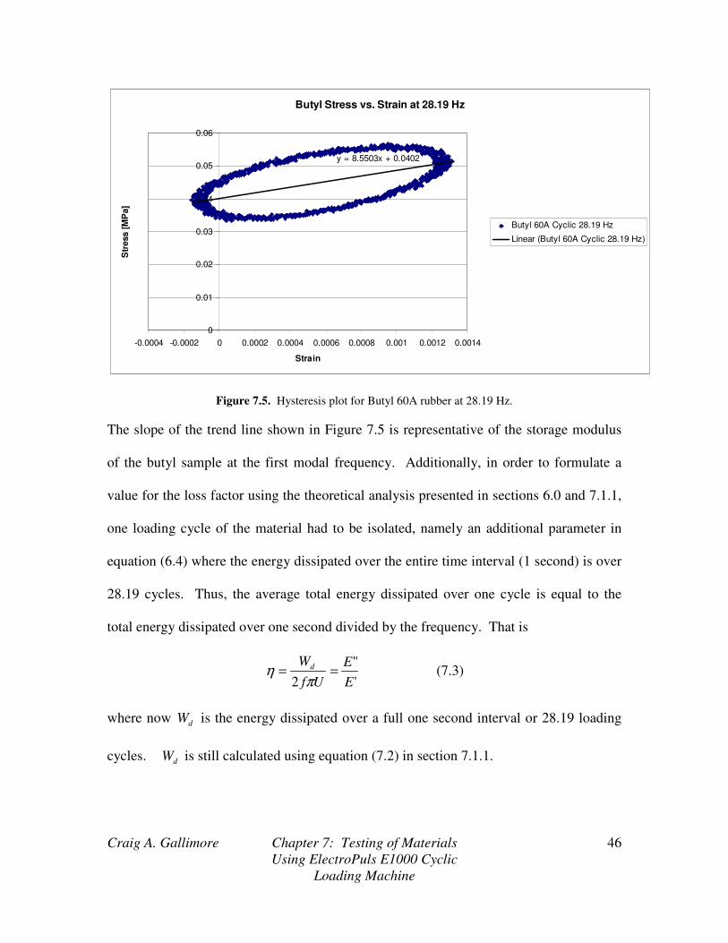
Craig A. Gallimore Chapter 7: Testing of Materials
Using ElectroPuls E1000 Cyclic
Loading Machine
46
Butyl Stress vs. Strain at 28.19 Hz
y = 8.5503x + 0.0402
0
0.01
0.02
0.03
0.04
0.05
0.06
-0.0004 -0.0002 0 0.0002 0.0004 0.0006 0.0008 0.001 0.0012 0.0014
Strain
Str
ess [
MP
a]
Butyl 60A Cyclic 28.19 Hz
Linear (Butyl 60A Cyclic 28.19 Hz)
Figure 7.5. Hysteresis plot for Butyl 60A rubber at 28.19 Hz.
The slope of the trend line shown in Figure 7.5 is representative of the storage modulus
of the butyl sample at the first modal frequency. Additionally, in order to formulate a
value for the loss factor using the theoretical analysis presented in sections 6.0 and 7.1.1,
one loading cycle of the material had to be isolated, namely an additional parameter in
equation (6.4) where the energy dissipated over the entire time interval (1 second) is over
28.19 cycles. Thus, the average total energy dissipated over one cycle is equal to the
total energy dissipated over one second divided by the frequency. That is
'
"
2 E
E
Uf
Wd ==π
η (7.3)
where now dW is the energy dissipated over a full one second interval or 28.19 loading
cycles. dW is still calculated using equation (7.2) in section 7.1.1.

Craig A. Gallimore Chapter 7: Testing of Materials
Using ElectroPuls E1000 Cyclic
Loading Machine
47
7.3 SBR 70A Rubber Testing
SBR rubber, short for styrene-butadiene rubber, is a synthetic copolymer rubber
developed in the 1930’s. It is produced in a similar polymerization process as butyl
rubbers, but of a slightly different molecular make-up. It is one of the more cost effect
rubbers to manufacture and was first produced to account for the dwindling natural
rubber resources. SBR rubber is used in automotive tires, belts and hoses, for machinery
and engines, gaskets, and break and clutch pads for vehicles. It is also often found in
some children’s toys, caulking compounds, sponges, and floor tiles. It is one of the more
widely produced rubbers in the world and, like butyl, was chosen for testing because of
its low cost and relatively high flexural and damping properties. From a manufacturing
standpoint, SBR is as easy to produce as butyl rubber, but often for a much cheaper price
because of the materials used and the fact that it is a copolymer, needing very little of the
more expensive rubber materials to make it an effective rubber.
As with the other six damping materials, a sample of SBR having rectangular
cross section was loaded into the ElectroPuls machine and loaded at 1, 5, 10, 15, and
28.19 Hz. Table 7.2 gives the storage moduli and loss factors at these frequencies.
Table 7.2. SBR stiffness and loss factor data for cyclic loading tests.
Frequency [Hz]
Storage Modulus
[MPa] Shear Modulus
[MPa] Loss
Factor
1 7.2807 2.476428571 0.0647
5 8.1663 2.777653061 0.0826
10 8.5415 2.905272109 0.09335
15 8.8745 3.018537415 0.1163
28.19 12.331 4.194217687 0.2374
Figure 7.6 gives a graphical representation of the data presented in Table 7.2.

Craig A. Gallimore Chapter 7: Testing of Materials
Using ElectroPuls E1000 Cyclic
Loading Machine
48
Modulus and Loss Factor Data for SBR 70A Rubber
0
2
4
6
8
10
12
14
0 5 10 15 20 25 30
Frequency
Sto
rag
e M
od
ulu
s [
MP
a]
0
0.05
0.1
0.15
0.2
0.25
Lo
ss
Fa
cto
r
Modulus Data [MPa]
Loss Factor
Figure 7.6. Storage Modulus and Loss Factor plot for SBR rubber as a function of frequency.
From Table 7.2 and Figure 7.6 it can be seen that, like butyl, there is a significant
increase in both the storage modulus and loss factor as the frequency is increased.
However, the maximum damping factor, the parameter of most significant interest, hits a
peak value of only .2374 within the testing frequency range. This value is about half that
of butyl, making it a relatively poor choice for a landing gear application when compared
to other materials tested. Notice, however, that the measured storage modulus values for
SBR are significantly higher than that for butyl. This is expected because the SBR has a
durometer rating of 70 shore A, while the butyl is rated at 60 on the A scale. It will also
be shown that SBR rubber has one of the largest values of storage modulus among the
other test materials at all frequencies tested. It follows that there is a trade-off between
stiffness and damping. If the stiffness of a structure is high, the natural damping of that
structure will inherently be low because the structure is prone to recover energy upon
unloading, making it more difficult to damp out unwanted vibrations. Fixed landing gear

Craig A. Gallimore Chapter 7: Testing of Materials
Using ElectroPuls E1000 Cyclic
Loading Machine
49
structures, like the one of interest, are generally very stiff. Metals are a perfect example
of high stiffness materials which have very low damping. Composites, however, are also
very stiff, often much stiffer than metals, yet they generally have higher damping because
of a multitude of different damping mechanisms such as interfacial damping and
frictional damping (Birman, 2002, Markley, 1988, Saravanos, 1991), which are outside
the scope of this report.
At the highest testing frequency of 28.19 Hz, the stress-strain plot for SBR 70A
rubber is shown in Figure 7.7.
SBR 70A Stress vs. Strain at 28.19 Hz
y = 12.331x + 0.0617
0
0.02
0.04
0.06
0.08
0.1
0.12
-0.0005 0 0.0005 0.001 0.0015 0.002 0.0025 0.003
Strain
Str
ess [
MP
a]
SBR 70A Cyclic 28.19 Hz
Linear (SBR 70A Cyclic 28.19 Hz)
Figure 7.7. Hysteresis plot of stress and strain for SBR 70A rubber at 28.19 Hz.
This figure was analyzed in the same manner as that of butyl rubber in the preceding
section, where the total energy dissipated over the one second test interval is divided by
Craig A. Gallimore Chapter 7: Testing of Materials
Using ElectroPuls E1000 Cyclic
Loading Machine
50
the number of cycles (28.19) and applied to the theory outlined in section 6.0. Again, the
elliptical shape of the plot, characteristic of viscoelastic materials, is shifted upwards due
to a small static preload of the test material prior to load cycling. Additionally, it can be
seen from Figure 7.7 that the SBR 70A rubber sample was cyclically loaded in tension
due to the positive strain values. There is a small portion of the data showing negative
strain, indicating a small portion of the loading history as compressive in nature.
7.4 Buna-N/Nitrile 40A Rubber Testing
Nitrile rubber, or Buna-N, is a synthetic copolymer rubber of acrylonitrile (ACN)
and butadiene. This type of rubber falls into the nitrile-butadiene family of rubbers
which consist of unsaturated copolymers of 2-propenenitrile and various butadiene
monomers including 1,2-butadiene and 1,3-butadiene. The varying compositions of
nitrile rubbers allow it to be very resistant to oils, fuels, and other chemicals. This makes
it an excellent material to manufacture rubber gloves. Additionally, nitrile rubbers are
used in the automotive industry to make oil handling hoses, seals, and grommets. Nitrile
rubber also has a wide temperature range (about -40 to +120 degrees Centigrade) making
it an excellent material choice for both high and low temperature applications. By
varying the composition of nitrile rubber, it can be made more resistant to oils and acids,
but will have inferior strength and flexibility. This aspect of nitrile rubbers makes it
particularly appealing for an aircraft landing gear application. During operation, the
material will undoubtedly come in contact with foreign substances such as oils, petrols
and fuels, and perhaps strong acids. Thus, a resistance to these foreign substances will
increase the longevity of such a damping material during operation, effectively
increasing the service life of the landing gear.

Craig A. Gallimore Chapter 7: Testing of Materials
Using ElectroPuls E1000 Cyclic
Loading Machine
51
Two samples of nitrile rubber, each having different durometers, were tested in
the ElectroPuls machine. This section presents storage moduli and loss factor data of a
nitrile rubber having a 40 durometer rating on the A scale. The sample was loaded at 1,
5, 10, 15, and 28.19 Hz. Table 7.3 gives the data taken from the experiments at the
frequency mentioned.
Table 7.3. Storage Modulus and Loss Factor data for Buna-N/Nitrile rubber 40A.
Frequency [Hz]
Storage Modulus
[MPa] Shear Modulus
[MPa] Loss
Factor
1 2.2917 0.779489796 0.047551
5 2.2487 0.764863946 0.06903
10 1.9368 0.65877551 0.0928
15 1.8604 0.632789116 0.15608
28.19 4.5533 1.548741497 1.0346
Figure 7.8 gives a graphical representation of the data in Table 7.3.
Modulus and Loss Factor Data for Nitrile 40A Rubber
0
0.5
1
1.5
2
2.5
3
3.5
4
4.5
5
0 5 10 15 20 25 30
Frequency
Sto
rag
e M
od
ulu
s [
MP
a]
0
0.2
0.4
0.6
0.8
1
1.2L
os
s F
ac
tor
Modulus Data [MPa]
Loss Factor
Figure 7.8. Storage Modulus and loss factor data for Buna-N/Nitrile rubber 40A.

Craig A. Gallimore Chapter 7: Testing of Materials
Using ElectroPuls E1000 Cyclic
Loading Machine
52
This plot shows some interesting trends not seen in either SBR or Butyl rubber data. At
lower frequency, the loss factor slowly rises while the storage modulus slowly falls. But
at the first modal frequency (28.19 Hz) of the undamped cantilever beam, there is a sharp
spike in both the storage modulus and loss factor of the material. This could indicate that
the material is entering its transition region where both the storage modulus and loss
factor rise until the loss factor hits a maximum value. Also, notice the large loss factor
and lower storage modulus of nitrile 40A when compared to either SBR 70A or Butyl
60A. The loss factor of nitrile 40A is over double that of butyl 60A and quadruple that of
SBR 70A at the first modal frequency. This makes the nitrile rubber the best material so
far for the damping of a landing gear system. Also, the high loss factors combined with
the environmental resistances of nitrile rubbers gives this family of rubbers excellent
applicability to a landing gear.
At the first modal frequency of the cantilever beam, the stress-strain plot for
nitrile 40A rubber is shown in Figure 7.9.

Craig A. Gallimore Chapter 7: Testing of Materials
Using ElectroPuls E1000 Cyclic
Loading Machine
53
Buna-N/Nitrile 40A Stress vs. Strain at 28.19 Hz
y = -4.5533x + 0.052
0
0.01
0.02
0.03
0.04
0.05
0.06
0.07
-0.002 -0.0015 -0.001 -0.0005 0 0.0005 0.001 0.0015
Strain
Str
ess [
MP
a]
Nitrile 40A Cyclic 28.19 Hz
Linear (Nitrile 40A Cyclic 28.19 Hz)
Figure 7.9. Hysteresis loop of stress and strain for nitrile 40A rubber.
This plot shows that the material was loaded in both tension and compression. It should
be noted that though the slope of the ellipse is negative from the trend line in Figure 7.9,
the absolute value of the trend line slope is the equivalent storage modulus of the material
at a given frequency. The data is mirrored because of a necessary change in reference
point in the ElectroPuls because of material sample dimensions. This data was analyzed
in the same fashion as the butyl rubber in section 7.2 where the data for a complete one
second time interval was used to find the total energy dissipated over that interval divided
by the number of cycles. This allows an average energy dissipation per cycle to be used
rather than isolating the data for any one cycle during the one second interval.
7.5 Buna-N/Nitrile 60A Rubber Testing
A second sample of nitrile rubber have a durometer of 60 on the A scale was also
tested. This sample of nitrile rubber offers the same environmental resistance properties
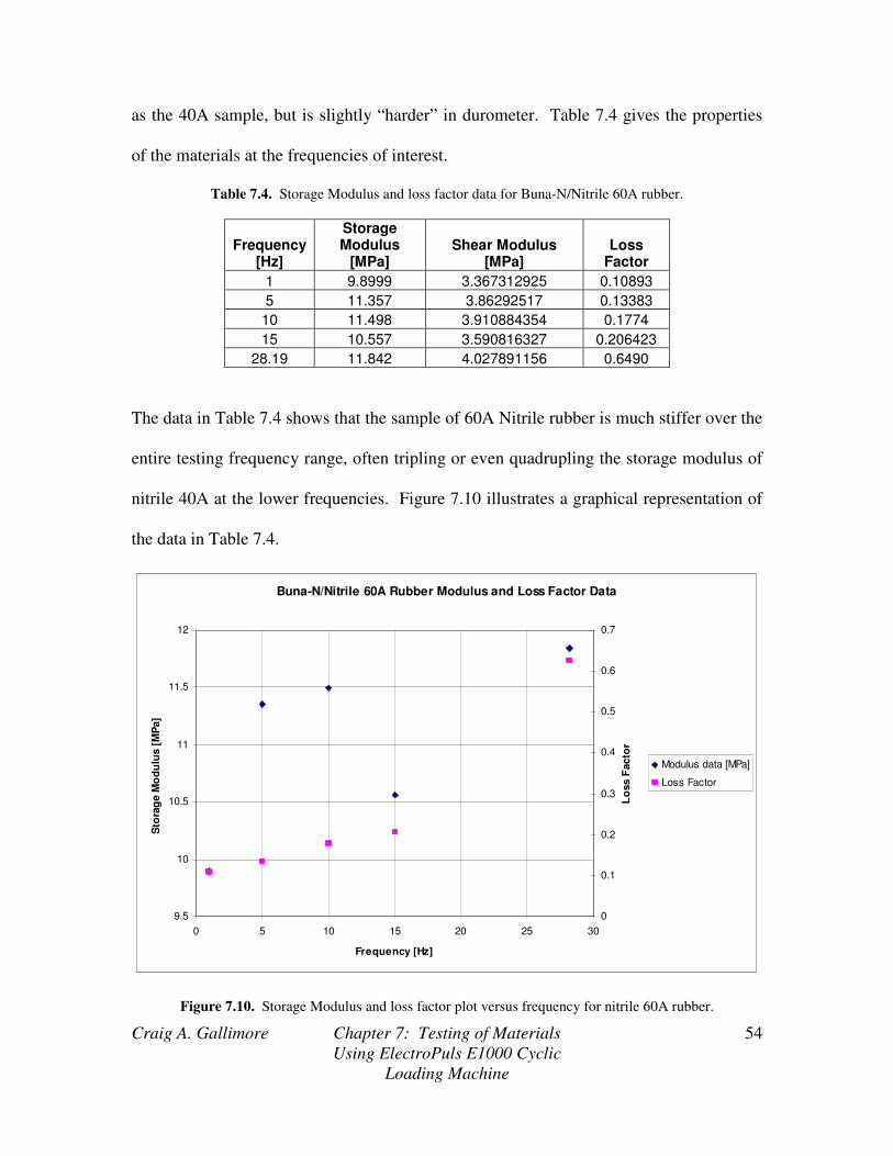
Craig A. Gallimore Chapter 7: Testing of Materials
Using ElectroPuls E1000 Cyclic
Loading Machine
54
as the 40A sample, but is slightly “harder” in durometer. Table 7.4 gives the properties
of the materials at the frequencies of interest.
Table 7.4. Storage Modulus and loss factor data for Buna-N/Nitrile 60A rubber.
Frequency [Hz]
Storage Modulus
[MPa] Shear Modulus
[MPa] Loss
Factor
1 9.8999 3.367312925 0.10893
5 11.357 3.86292517 0.13383
10 11.498 3.910884354 0.1774
15 10.557 3.590816327 0.206423
28.19 11.842 4.027891156 0.6490
The data in Table 7.4 shows that the sample of 60A Nitrile rubber is much stiffer over the
entire testing frequency range, often tripling or even quadrupling the storage modulus of
nitrile 40A at the lower frequencies. Figure 7.10 illustrates a graphical representation of
the data in Table 7.4.
Buna-N/Nitrile 60A Rubber Modulus and Loss Factor Data
9.5
10
10.5
11
11.5
12
0 5 10 15 20 25 30
Frequency [Hz]
Sto
rag
e M
od
ulu
s [
MP
a]
0
0.1
0.2
0.3
0.4
0.5
0.6
0.7L
oss F
acto
r
Modulus data [MPa]
Loss Factor
Figure 7.10. Storage Modulus and loss factor plot versus frequency for nitrile 60A rubber.
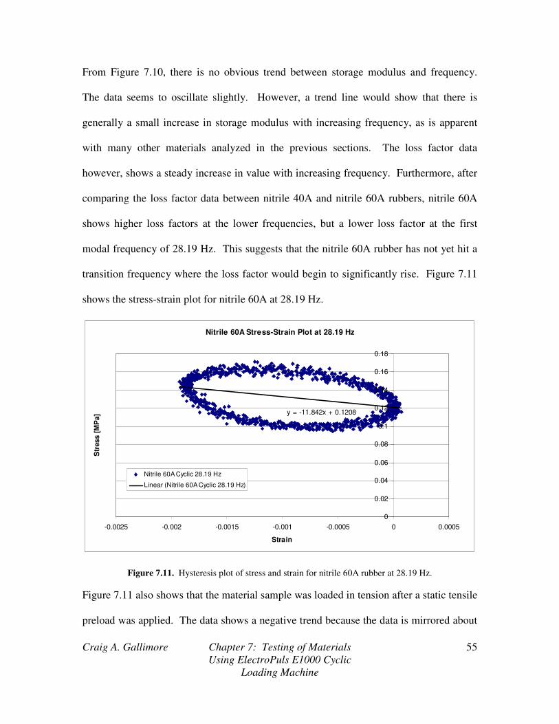
Craig A. Gallimore Chapter 7: Testing of Materials
Using ElectroPuls E1000 Cyclic
Loading Machine
55
From Figure 7.10, there is no obvious trend between storage modulus and frequency.
The data seems to oscillate slightly. However, a trend line would show that there is
generally a small increase in storage modulus with increasing frequency, as is apparent
with many other materials analyzed in the previous sections. The loss factor data
however, shows a steady increase in value with increasing frequency. Furthermore, after
comparing the loss factor data between nitrile 40A and nitrile 60A rubbers, nitrile 60A
shows higher loss factors at the lower frequencies, but a lower loss factor at the first
modal frequency of 28.19 Hz. This suggests that the nitrile 60A rubber has not yet hit a
transition frequency where the loss factor would begin to significantly rise. Figure 7.11
shows the stress-strain plot for nitrile 60A at 28.19 Hz.
Nitrile 60A Stress-Strain Plot at 28.19 Hz
y = -11.842x + 0.1208
0
0.02
0.04
0.06
0.08
0.1
0.12
0.14
0.16
0.18
-0.0025 -0.002 -0.0015 -0.001 -0.0005 0 0.0005
Strain
Str
ess [
MP
a]
Nitrile 60A Cyclic 28.19 Hz
Linear (Nitrile 60A Cyclic 28.19 Hz)
Figure 7.11. Hysteresis plot of stress and strain for nitrile 60A rubber at 28.19 Hz.
Figure 7.11 also shows that the material sample was loaded in tension after a static tensile
preload was applied. The data shows a negative trend because the data is mirrored about

Craig A. Gallimore Chapter 7: Testing of Materials
Using ElectroPuls E1000 Cyclic
Loading Machine
56
the stress axis due to a change in reference point caused by the dimensions of the sample.
From this plot, a storage modulus of 11.842 MPa and a loss factor of .6490 were found
by using the theory presented in section 6.0. Between the nitrile, butyl, and SBR rubbers
which have been analyzed, both of the nitrile rubber samples hold the highest loss factor
values at the first modal frequency.
7.6 Silicone 30A Rubber Testing
Silicone rubber is a polymer that has a backbone of silicone-oxygen bonds, the
same bond found in quartz, glass, and sand. Silicone rubbers offer good temperature
resistance, often having operational temperatures from -55 to +300 degrees centigrade.
Silicone rubber is also resistant to ozone, and ultraviolet radiation, making it an elastomer
of choice for extreme environments. However, silicone rubbers often have very low
tensile strength, making it less desirable for applications involving high loads.
A sample of silicone 30A rubber was loaded into the ElectroPuls machine and
tested at 1, 5, 10, 15, and 28.19 Hz. By physical inspection, silicone 30A rubber is very
“sponge-like” and easily manipulated by applying small hand loads. This is contrary to
many of the other rubbers, all of which have much higher durometers. Upon loading of
silicone 30A in the ElectroPuls, load and position data was gathered and was used to
generate the storage modulus and loss factor data summarized in Table 7.5.
Table 7.5. Storage Modulus and loss factor data for silicone 30A rubber.
Frequency [Hz]
Storage Modulus
[MPa] Shear Modulus
[MPa] Loss
Factor
1 4.8319 1.643503401 0.0916
5 4.1329 1.405748299 0.056277
10 4.1077 1.397176871 0.06234
15 3.9549 1.345204082 0.07847
28.19 0.9363 0.318469388 1.4316

Craig A. Gallimore Chapter 7: Testing of Materials
Using ElectroPuls E1000 Cyclic
Loading Machine
57
Additionally, Figure 7.12 shows the storage modulus and loss factor data for silicone 30A
plotted against frequency.
Silicone 30A Modulus and Loss Factor Data
0
1
2
3
4
5
6
0 5 10 15 20 25 30
Frequency [Hz]
Sto
rag
e M
od
ulu
s [
MP
a]
0
0.2
0.4
0.6
0.8
1
1.2
1.4
1.6
Lo
ss F
acto
r
Modulus Data [MPa]
Loss Factor
Figure 7.12. Storage Modulus and loss factor data for silicone 30A rubber.
This plot shows a relationship between storage modulus, loss factor, and frequency unlike
any of the materials analyzed in the previous sections. As the frequency increases, the
storage modulus shows a significant decrease, where the modulus values are the lowest of
any material tested. The loss factor slowly increases with frequency and then spikes
sharply at or around 28.19 Hz. The loss factor data for silicone 30A is among the lowest
of any material tested at lower frequency, and then spikes to a value at 28.19 Hz more
than 14 times the initial loss factor value at 1 Hz. This indicates that silicone rubber is
perhaps the best damping material analyzed, having high loss factors and very low

Craig A. Gallimore Chapter 7: Testing of Materials
Using ElectroPuls E1000 Cyclic
Loading Machine
58
moduli, giving a large ratio of imaginary to real parts of the complex modulus. Figure
7.13 shows the cyclic loading behavior of silicone 30A at 28.19 Hz.
Silicone 30A Stress-Strain Plot at 28.19 Hz
y = 0.9363x + 0.0504
0
0.01
0.02
0.03
0.04
0.05
0.06
0.07
-0.003 -0.0025 -0.002 -0.0015 -0.001 -0.0005 0 0.0005
Strain
Str
ess [
MP
a]
Silicone 30A Cyclic 28.19 Hz
Linear (Silicone 30A Cyclic 28.19 Hz)
Figure 7.13. Silicone 30A cyclic stress versus strain relationship at 28.19 Hz.
Due to the negative strain values, the silicone 30A material sample was loaded in
compression after a tensile static preload was applied. Rather, the material was preloaded
in tension and then allowed to relax slightly to generate the plot in Figure 7.13. The loss
factor at 28.19 Hz was higher than any other material tested, more than double the loss
factor of nitrile 60A rubber and about 1.4 times the loss factor of nitrile 40A rubber.
As a final note on silicone 30A, during testing for one cycle at 1, 5, 10, and 15
Hz, the material showed a fairly significant nonlinear loading behavior, shown in Figure
7.14.

Craig A. Gallimore Chapter 7: Testing of Materials
Using ElectroPuls E1000 Cyclic
Loading Machine
59
Silicone 30A Stress-Strain Plot for 10 Hz
-0.05
0
0.05
0.1
0.15
0.2
0.25
0.3
-0.01 0 0.01 0.02 0.03 0.04 0.05 0.06 0.07 0.08
Strain
Str
ess [
MP
a]
Silicone 30A 10 Hz
Figure 7.14. Example of loading nonlinearity of silicone 30A rubber.
This figure shows a loading behavior which has both loading (top curve) and unloading
(bottom curve) as concave upwards. For most viscoelastic materials tested in this report,
the loading behavior was that of Figure 7.1, where the loading curve was concave down
and the unloading curve was concave up, forming an ellipse. Because of this unusual
behavior relative to the other materials in the report, an average storage modulus was
calculated. This average storage modulus was the slope from the preload origin to the
maximum load point in the loading curve (point of maximum strain). This average
modulus value was then used in equation (6.4) to calculate the loss factor. The energy
dissipated during the cycle, however, was calculated in the same fashion as all other
materials.

Craig A. Gallimore Chapter 7: Testing of Materials
Using ElectroPuls E1000 Cyclic
Loading Machine
60
The nonlinear behavior in Figure 7.14 is most likely caused by the relatively large
strain amplitudes. Most viscoelastic materials exhibit nonlinearity at large cyclic strain
amplitudes, as discussed in section 2.2.1.3. The maximum elongations seen in the
silicone 30A test sample for loading at 1, 5, 10, and 15 Hz were on the order of 5-8%,
resulting in all plots showing varying degrees of nonlinearity. However, for 28.19 Hz,
the cyclic strain amplitudes were very low, having a maximum elongation between .2-
.3%, about 25 times lower than tests at lower frequencies. The low strains seen in the
28.19 Hz test result in linear behavior.
7.7 Silicone 50A Rubber Testing
A sample of silicone 50A rubber was also tested using the ElectroPuls machine.
This sample of silicone rubber had a slightly higher durometer of 50A and exhibited
greatly decreased damping when compared to the silicone 30A sample. Table 7.6 gives
the storage modulus and damping value for silicone 50A at 1, 5, 10, 15, and 28.19 Hz.
Table 7.6. Silicone 50A modulus and loss factor data.
Frequency [Hz]
Storage Modulus
[MPa] Shear Modulus
[MPa] Loss
Factor
1 2.8811 0.979965986 0.0263
5 2.7351 0.930306122 0.03476
10 2.468 0.839455782 0.043799
15 1.6567 0.563503401 0.10541
28.19 2.8274 0.96170068 0.37729
These results are further illustrated in Figure 7.15.

Craig A. Gallimore Chapter 7: Testing of Materials
Using ElectroPuls E1000 Cyclic
Loading Machine
61
Silicone 50A Modulus and Loss Factor Data
0
0.5
1
1.5
2
2.5
3
3.5
0 5 10 15 20 25 30
Frequency
Sto
rag
e M
od
ulu
s [
MP
a]
0
0.05
0.1
0.15
0.2
0.25
0.3
0.35
0.4
Lo
ss F
acto
r
Modulus Data [MPa]
Loss Factor
Figure 7.15. Storage Modulus and loss factor data for silicone 50A rubber.
Figure 7.15 shows a steady decrease in storage modulus with increasing frequency from 1
to 15 Hz. However, the storage modulus spikes at or around 28.19 Hz. The loss factor
shows a steady increase with increasing frequency. This suggests that the material has
not yet entered the transition region. The maximum loss factor found was .37729 at
28.19 Hz. This loss factor is lower than that of its silicone 30A counterpart, butyl, and
both nitrile rubbers. The shear modulus, however, is still much lower than butyl and both
nitrile rubbers. The predicted effectiveness of silicone 50A will be compared to the other
damping materials in Chapter 8.
Like all other materials analyzed in the preceding sections, the maximum loss
factor was found at the highest frequency corresponding to the first modal frequency of
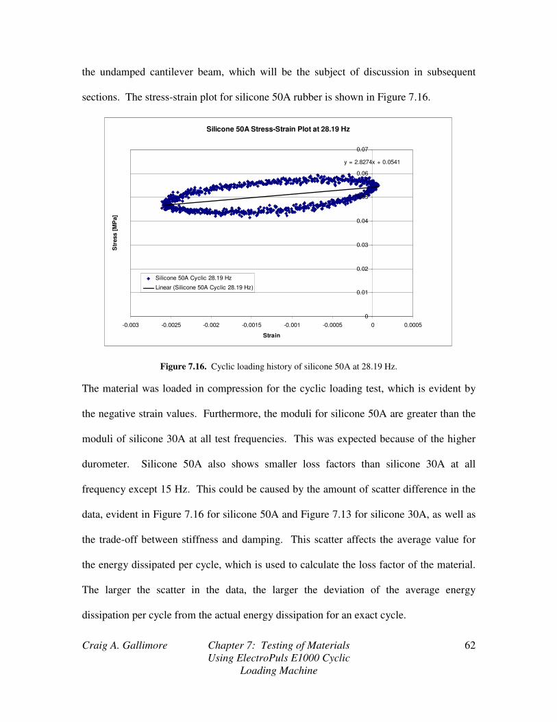
Craig A. Gallimore Chapter 7: Testing of Materials
Using ElectroPuls E1000 Cyclic
Loading Machine
62
the undamped cantilever beam, which will be the subject of discussion in subsequent
sections. The stress-strain plot for silicone 50A rubber is shown in Figure 7.16.
Silicone 50A Stress-Strain Plot at 28.19 Hz
y = 2.8274x + 0.0541
0
0.01
0.02
0.03
0.04
0.05
0.06
0.07
-0.003 -0.0025 -0.002 -0.0015 -0.001 -0.0005 0 0.0005
Strain
Str
ess [
MP
a]
Silicone 50A Cyclic 28.19 Hz
Linear (Silicone 50A Cyclic 28.19 Hz)
Figure 7.16. Cyclic loading history of silicone 50A at 28.19 Hz.
The material was loaded in compression for the cyclic loading test, which is evident by
the negative strain values. Furthermore, the moduli for silicone 50A are greater than the
moduli of silicone 30A at all test frequencies. This was expected because of the higher
durometer. Silicone 50A also shows smaller loss factors than silicone 30A at all
frequency except 15 Hz. This could be caused by the amount of scatter difference in the
data, evident in Figure 7.16 for silicone 50A and Figure 7.13 for silicone 30A, as well as
the trade-off between stiffness and damping. This scatter affects the average value for
the energy dissipated per cycle, which is used to calculate the loss factor of the material.
The larger the scatter in the data, the larger the deviation of the average energy
dissipation per cycle from the actual energy dissipation for an exact cycle.
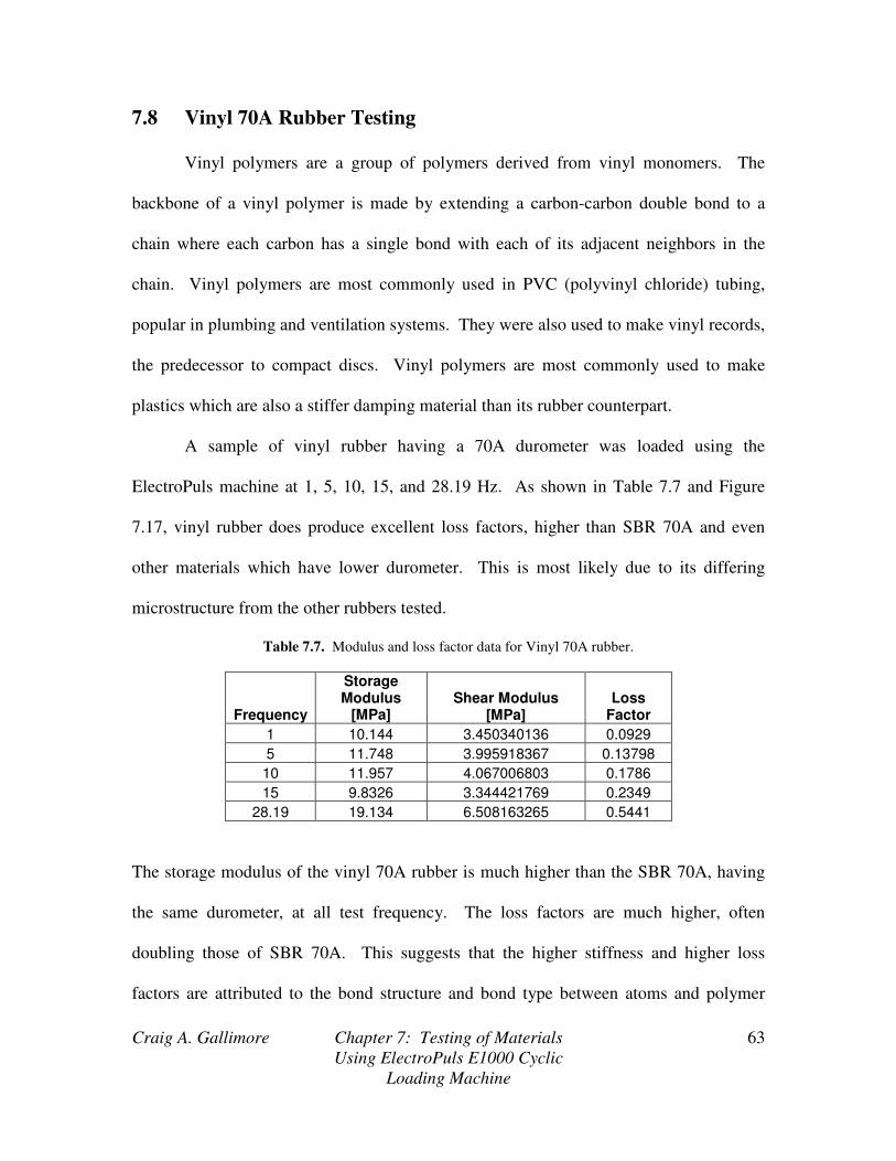
Craig A. Gallimore Chapter 7: Testing of Materials
Using ElectroPuls E1000 Cyclic
Loading Machine
63
7.8 Vinyl 70A Rubber Testing
Vinyl polymers are a group of polymers derived from vinyl monomers. The
backbone of a vinyl polymer is made by extending a carbon-carbon double bond to a
chain where each carbon has a single bond with each of its adjacent neighbors in the
chain. Vinyl polymers are most commonly used in PVC (polyvinyl chloride) tubing,
popular in plumbing and ventilation systems. They were also used to make vinyl records,
the predecessor to compact discs. Vinyl polymers are most commonly used to make
plastics which are also a stiffer damping material than its rubber counterpart.
A sample of vinyl rubber having a 70A durometer was loaded using the
ElectroPuls machine at 1, 5, 10, 15, and 28.19 Hz. As shown in Table 7.7 and Figure
7.17, vinyl rubber does produce excellent loss factors, higher than SBR 70A and even
other materials which have lower durometer. This is most likely due to its differing
microstructure from the other rubbers tested.
Table 7.7. Modulus and loss factor data for Vinyl 70A rubber.
Frequency
Storage Modulus
[MPa] Shear Modulus
[MPa] Loss
Factor
1 10.144 3.450340136 0.0929
5 11.748 3.995918367 0.13798
10 11.957 4.067006803 0.1786
15 9.8326 3.344421769 0.2349
28.19 19.134 6.508163265 0.5441
The storage modulus of the vinyl 70A rubber is much higher than the SBR 70A, having
the same durometer, at all test frequency. The loss factors are much higher, often
doubling those of SBR 70A. This suggests that the higher stiffness and higher loss
factors are attributed to the bond structure and bond type between atoms and polymer

Craig A. Gallimore Chapter 7: Testing of Materials
Using ElectroPuls E1000 Cyclic
Loading Machine
64
chains within a rubber. Thus, the ability of a material to damp out vibrations and
dissipate energy is highly dependent on the microstructure and type of the material.
Vinyl 70A Modulus and Loss Factor Data
0
5
10
15
20
25
0 5 10 15 20 25 30
Frequency
Sto
rag
e M
od
ulu
s [
MP
a]
0
0.1
0.2
0.3
0.4
0.5
0.6
Lo
ss F
acto
r
Modulus Data [MPa]
Loss Factor
Figure 7.17. Storage modulus and loss factor data for vinyl 70A rubber.
From Figure 7.17 and Table 7.7, the storage modulus increases from 9.8 to 12 MPa from
1 to 15 Hz. But at 28.19 Hz the storage modulus jumps significantly by over 7 MPa. The
loss factor, however, shows a fairly linear trend with frequency. Because the vinyl
rubber is very stiff, but has only moderately high loss factors, the ratio of loss factor to
shear modulus is still relatively low when compared to the other materials.
Vinyl 70A rubber has the fourth highest loss factor at 28.19 Hz and is bettered
only by silicone 30A, nitrile 40A, and nitrile 60A out of the seven materials tested on the
ElectroPuls cyclic loading machine. However, it is also the stiffest material tested at

Craig A. Gallimore Chapter 7: Testing of Materials
Using ElectroPuls E1000 Cyclic
Loading Machine
65
28.19 Hz, suggesting that it will not offer as much damping performance as polymers
which have about the same loss factor, but much smaller shear modulus.
7.9 Soundcoat Dyad Material Data
All seven of the materials loaded in the ElectroPuls cyclic loading machine were
common rubbers available at almost any polymer distributor. Soundcoat Company
produces specialty products for acoustical and vibration damping applications.
Soundcoat Dyad is a line of product having three different grades, namely Dyad 601,
Dyad 606, and Dyad 609. Each grade is intended for different temperature ranges, with
Dyad 601 for lower temperatures and Dyad 609 for the upper extreme temperatures.
Typical applications of Soundcoat Dyad are marine applications with steel and aluminum
vessels, electronic equipment like disk drives and mass storage systems, engines and
transmissions, machine tools, and aerospace and aircraft applications.
Soundcoat Dyad offers some unique benefits which many other specialty
materials do not. Dyad will damp any thickness of metal while achieving significantly
high loss factors. It has excellent chemical and heat resistance. The three grades can also
be combined (laminated) to broaden the effective damping temperature range. For
instance, grades 601, 606, and 609 can be bonded back to back to achieve significant
damping levels over a broader temperature range than any one material alone, effectively
combining each materials operating temperature range with the other two materials. For
instance, if all three materials were laminated and tested at a single frequency as the
temperature was slowly increased, at least one laminate layer would always be in its
transition region, offering maximum damping. The other two materials would be
operating in either a glassy region, if the testing temperature was less than the minimum
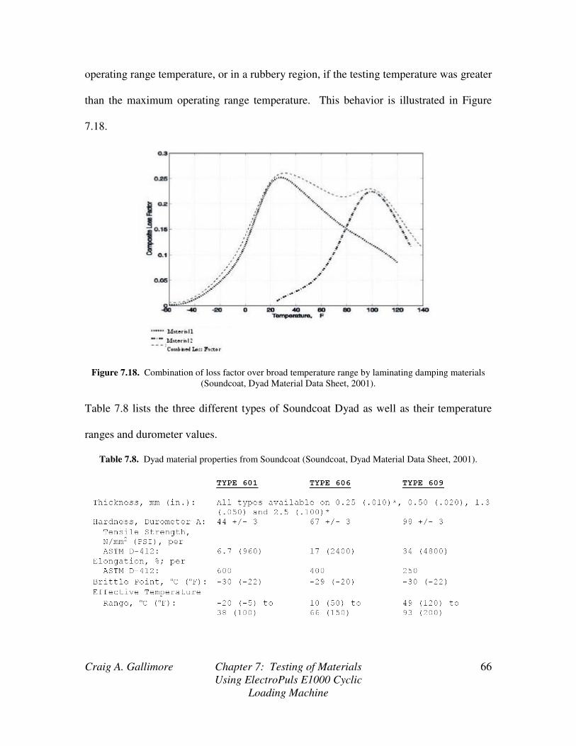
Craig A. Gallimore Chapter 7: Testing of Materials
Using ElectroPuls E1000 Cyclic
Loading Machine
66
operating range temperature, or in a rubbery region, if the testing temperature was greater
than the maximum operating range temperature. This behavior is illustrated in Figure
7.18.
Figure 7.18. Combination of loss factor over broad temperature range by laminating damping materials
(Soundcoat, Dyad Material Data Sheet, 2001).
Table 7.8 lists the three different types of Soundcoat Dyad as well as their temperature
ranges and durometer values.
Table 7.8. Dyad material properties from Soundcoat (Soundcoat, Dyad Material Data Sheet, 2001).
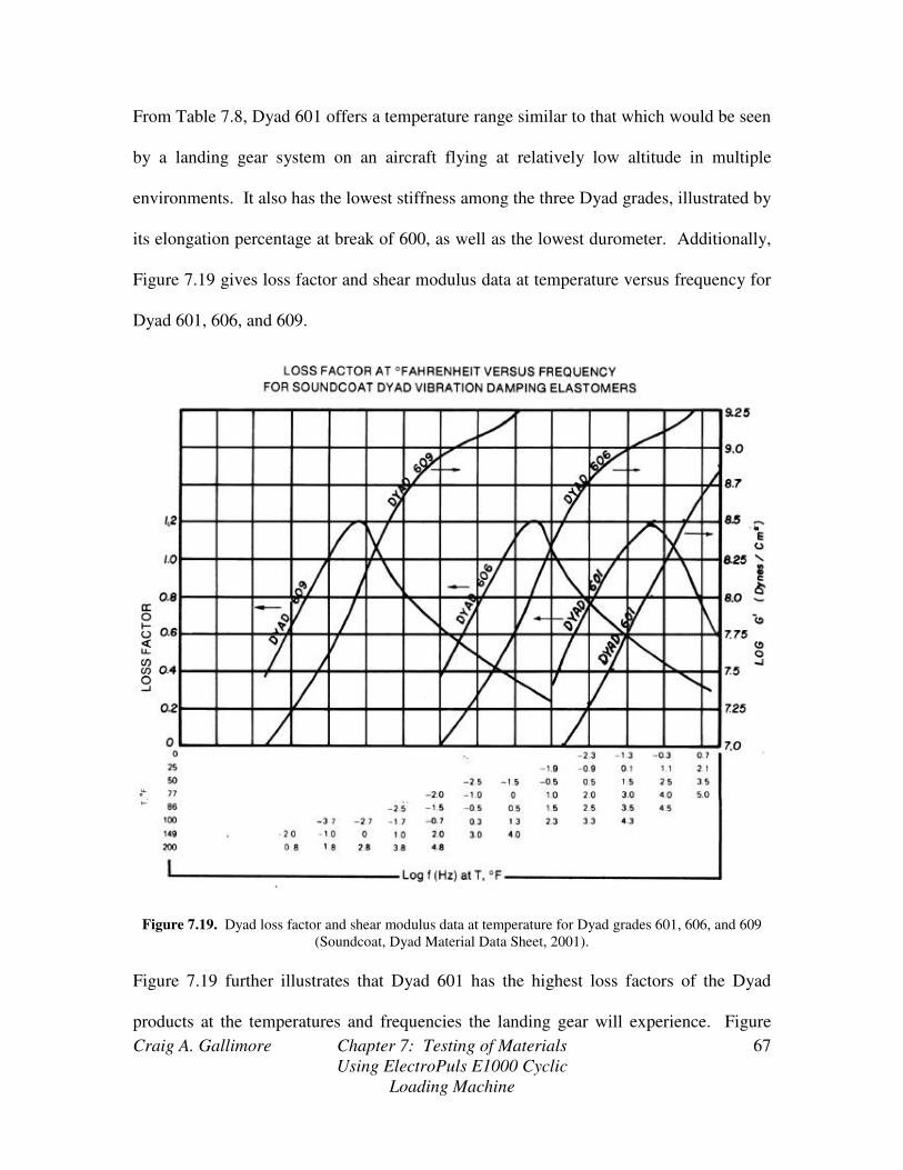
Craig A. Gallimore Chapter 7: Testing of Materials
Using ElectroPuls E1000 Cyclic
Loading Machine
67
From Table 7.8, Dyad 601 offers a temperature range similar to that which would be seen
by a landing gear system on an aircraft flying at relatively low altitude in multiple
environments. It also has the lowest stiffness among the three Dyad grades, illustrated by
its elongation percentage at break of 600, as well as the lowest durometer. Additionally,
Figure 7.19 gives loss factor and shear modulus data at temperature versus frequency for
Dyad 601, 606, and 609.
Figure 7.19. Dyad loss factor and shear modulus data at temperature for Dyad grades 601, 606, and 609
(Soundcoat, Dyad Material Data Sheet, 2001).
Figure 7.19 further illustrates that Dyad 601 has the highest loss factors of the Dyad
products at the temperatures and frequencies the landing gear will experience. Figure
Craig A. Gallimore Chapter 7: Testing of Materials
Using ElectroPuls E1000 Cyclic
Loading Machine
68
7.19 was generated by Soundcoat Company, so the testing of material samples in the
ElectroPuls machine was not necessary.
When loaded at 28.19 Hz at 77 degrees Fahrenheit, Figure 7.19 shows that Dyad
601 has a loss factor of =η .6 and LOG G’ = 7.1 2
cm
dynes (1.259 MPa). Dyad 601 has a
material loss factor closest to Buna-N/Nitrile 60A rubber, but a shear modulus closest to
Buna-N/Nitrile 40A. This makes Dyad 601 the material with the third highest damping
performance of all materials in this report. However, nitrile 40A rubber is still predicted
to produce higher composite system loss factors because of its smaller shear modulus at
28.19 Hz.
7.10 Damping Material Conclusions
Per the cyclic loading tests using the ElectroPuls machine and the Dyad loss
factor data courtesy of Soundcoat Co., the best viscoelastic damping materials were
selected for testing using the cantilever beam system discussed in section 5.0. It was
found that not only was the loss factor important in determining the damping
performance of a material, but the storage and shear moduli were equally as important, as
they help form the real part of a complex flexural rigidity formulated by the RKU
equations. Thus, materials which have high loss factors and low shear modulus are
desired for a landing gear application because the ratio of imaginary to real parts of the
complex flexural rigidity will be maximized. The following section is dedicated to
isolating the three best damping materials per the data collected via the cyclic loading
tests and to compare the predictions of the RKU equations to an experimental cantilever
beam test where actual materials are applied to a cantilever beam and tested.

Craig A. Gallimore Chapter 8: MATLAB Predictions and Trends
69
Chapter 8
MATLAB Predictions and Trends
In this section, a simple MATLAB program utilizing the Ross, Kerwin, and
Ungar equations for a damped cantilever beam is used to predict the loss factor using
Soundcoat’s Dyad 601, Buna-N/Nitrile 40A, and silicone 30A, the best damping
materials found by cyclic loading tests. These materials were found to be the best
materials to apply to a landing gear because they produce the highest composite system
loss factors of all eight materials for a viscoelastic layer thickness between 1 and 3
millimeters. This fact is shown in Figure 8.1, where the composite system (host
structure, damping material, and constraining layer) loss factor is plotted against
viscoelastic layer thickness using RKU analysis and the MATLAB program found in
Appendix A for reference.
Figure 8.1. Cantilever Beam loss factor versus viscoelastic layer thickness for all damping materials
Craig A. Gallimore Chapter 8: MATLAB Predictions and Trends
70
The MATLAB program takes inputs of shear modulus and elastic modulus in units of
Pascals, thickness of the host structure, thickness of the constraining layer, and width of
the constraining layer, in this case the same dimension as the thickness of the host beam.
In Figure 8.1, the constraining layer is 1.31 mm and is the same for all materials.
The program generates a plot of damping factor of the composite system as a
function of the thickness of the damping layer for the three best damping materials of
sections 7.1 through 7.9, namely Dyad 601, Buna-N/Nitrile 40A, and Silicone 30A
rubber. All plots and figures are for the first modal frequency of the cantilever beam.
Furthermore, a short analysis of how the thickness and stiffness of the constraining layer
affects composite loss factor will be given at the end of the MATLAB predictions for the
damping materials. For sections 8.1 through 8.3, the host structure thickness is .375
inches (.0095 m), thickness of the constraining layer varies between .8 mm (.0008 m) and
.96 mm (.00096 m), and the elastic moduli of the host structure and constraining layer are
209 GPa (4140 Steel) and 68 GPa (Aluminum T0), respectively. Furthermore, the
damping treatment was only applied to one side of the cantilever beam prior to testing. If
another constrained treatment were applied to the opposite side of the beam, resulting in a
symmetric damping treatment, the damping would effectively double.
8.1 Using the RKU Equations to Predict Damping
Being able to predict effective damping of a structure pre-fabrication is a
necessary process when dealing with structural damping. This section is dedicated to
showing how the RKU equations can be used for a cantilever beam with a tip mass equal
to the mass of the beam. By definition, the RKU equations, given in equation sets (3.1),

Craig A. Gallimore Chapter 8: MATLAB Predictions and Trends
71
(3.2), and (3.3) and below for convenience, formulate a complex flexural rigidity of a
damped constrained layer beam system
+
−
−+
−−
−+−+
++
−−++=
)1(
)()(
2
)(
)()(
)1(
)(12
121212)*(
*
*
22*
2
*
2
33*3
v
cc
vsvv
ccvsvv
ss
v
cv
ccvvss
g
DdDdhE
DhhE
DdhEDhhE
DhEg
DdhE
hEhEhEEI
ss
nss
n
nncvc
v
vcc
v
v
cs
v
vs
vs
ccsvssv
vv
ss
ccvsvvvvsvv
IE
Lbh
ChhE
LG
phhE
Gg
hhhd
hhh
hEhEhEghE
hE
dhEhhEgd
hhE
D
42
4
2
2*
2
1
*
*
**
*
***
2
2
)(2
)()2
(
ωρξ
ξ
=
==
++=
+=
++++
++−=
Additionally, rη is the modal loss factor associated with*
vG . The loss modulus is
dependent on the mode because of frequency dependence on loss modulus. To find the
loss factor of the composite system (host beam, damping layer, and constraining layer),
one only need take the ratio of the imaginary to real parts of the complex flexural rigidity
(Hao, 2005), namely
)(Re
)(Im*
*
EIal
EIagcomposite =η (8.1)
Craig A. Gallimore Chapter 8: MATLAB Predictions and Trends
72
This loss factor now incorporates the loss factor of the damping material into dynamics of
the composite system, effectively giving an approximation of the rate of energy loss per
cycle of the composite system. Thus, the complex moduli and loss factor data for the
damping materials tested in this report can be used to find the loss factor of a cantilever
beam system.
8.2 Dyad 601 Damping Prediction
The parameters taken from Figure 7.18 for Dyad 601 at 28.19 Hz and 77 degrees
Fahrenheit where used as inputs into the RKU equations in the MATLAB program.
These parameters are a loss factor of 6.=η and a shear modulus of LOG G’ = 7.1
2cm
dynes (G’=1.259 MPa). Figure 8.2 shows the trend between damping layer thickness
and composite loss factor for a steel cantilever beam with an aluminum constraining
layer. The figure presented shows the predicted loss factor for the system used in the
tests: a host beam of 3/8” (9.53 mm) square 4140 steel rod, and a .96 mm by 9.53 mm
constraining layer.

Craig A. Gallimore Chapter 8: MATLAB Predictions and Trends
73
Figure 8.2. Cantilever beam loss factor as a function of Dyad 601 thickness.
This plot shows that for relatively small initial increases from .5 mm of the viscoelastic
layer thickness, there are significant increases in damping up to about 2 mm. After the
thickness of the damping layer passes 2 mm, the increases in damping begin to taper off
slightly as the viscoelastic layer thickness is increased. This suggests that more
significant damping increases can be gained without much weight addition to the landing
gear for thin viscoelastic layers (~.5mm – 2mm).
8.3 Silicone 30A Damping Prediction
The material properties found in section 7.6 were used as inputs into the
MATLAB prediction program. The results of the MATLAB prediction are shown in
Figure 8.3. The RKU equations predict very sharp increases in loss factor for small
increases in damping layer thickness for low thickness damping layers, about .5mm to

Craig A. Gallimore Chapter 8: MATLAB Predictions and Trends
74
2mm. This rapid increase in loss factor at low viscoelastic layer thicknesses is much
more pronounced than for Dyad 601. Thus, the most significant increases in damping
will occur for low additions in weight caused by the damping layer to the cantilever
beam.
Figure 8.3. RKU Prediction of cantilever beam loss factor as a function of damping layer thickness for
silicone 30A rubber.
To generate Figure 8.3, the constraining layer thickness was measured to be .8mm rather
than .96mm as for Dyad 601. In the following chapter where cantilever beam tests are
analyzed, the constraining layer thickness of the MATLAB prediction exactly matches
that of the beam tests.

Craig A. Gallimore Chapter 8: MATLAB Predictions and Trends
75
8.4 Buna-N/Nitrile 40A Damping Prediction
The material properties for Buna-N/Nitrile 40A found in section 7.4 at the first
modal frequency of the cantilever beam were used as inputs to the RKU MATLAB
program to generate a loss factor prediction as a function of viscoelastic layer thickness.
Figure 8.4 shows the resulting trend. Unlike the silicone 30A prediction in the preceding
section, there is no significant increase in loss factor for small increases in damping layer
thickness, but instead a steady increasing trend of loss factor with increasing damping
layer thickness.
Figure 8.4. Loss factor trend for cantilever beam system as a function of viscoelastic layer thickness for
Buna-N/Nitrile 40A rubber.
Like the silicone 30A prediction, a constraining layer thickness of .8 mm was used to
generate Figure 8.4. It is evident from Figure 8.4 that nitrile 40A rubber produces the

Craig A. Gallimore Chapter 8: MATLAB Predictions and Trends
76
lowest loss factors for low damping layer thickness and the highest loss factors for
thicker damping layers. Thus, it is a better material to use for applications where a
thicker damping layer is required. For a landing gear application however, nitrile 40A
will be the least effective damping material between Dyad 601 and Silicone 30A because
the damping layer should be kept as thin as possible while still achieving maximum
damping for low increases in gear weight.
8.5 Constraining Layer Effects on Beam Loss Factors
This section analyzes how the constraining layer modulus of elasticity and
thickness affect the composite system loss factor while keeping the material properties of
the viscoelastic damping layer constant. Figure 8.5 shows the general trends of system
loss factor as a function of variable constraining layer thickness and modulus of
elasticity. For variable thickness, the plot was generated using silicone 30A complex
modulus properties, a constraining layer elastic modulus of 68 GPa, and a frequency of
28.19 Hz. For variable constraining layer elastic modulus, the plot was generated using
silicone 30A complex modulus properties, a constraining layer thickness of 1.31 mm, and
a frequency of 28.19 Hz.
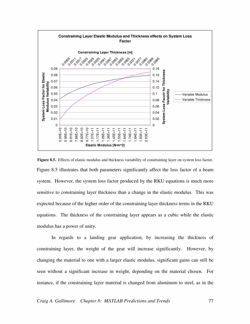
Craig A. Gallimore Chapter 8: MATLAB Predictions and Trends
77
Constraining Layer Elastic Modulus and Thickness effects on System Loss
Factor
0
0.01
0.02
0.03
0.04
0.05
0.06
0.07
0.08
0.09
5.0
0E
+1
0
5.9
5E
+1
0
6.9
1E
+1
0
7.8
6E
+1
0
8.8
2E
+1
0
9.7
7E
+1
0
1.0
7E
+1
1
1.1
7E
+1
1
1.2
6E
+1
1
1.3
6E
+1
1
1.4
5E
+1
1
1.5
5E
+1
1
1.6
4E
+1
1
1.7
4E
+1
1
1.8
4E
+1
1
1.9
3E
+1
1
2.0
3E
+1
1Elastic Modulus [N/m^2]
Sy
ste
m L
os
s F
ac
tor
for
Ela
sti
c
Mo
du
lus
Va
ria
bil
ity
0
0.02
0.04
0.06
0.08
0.1
0.12
0.14
0.16
0.180.
0005
0.00
11
0.00
17
0.00
23
0.00
29
0.00
35
0.00
41
0.00
47
0.00
53
0.00
59
0.00
65
0.00
71
0.00
77
0.00
83
0.00
89
0.00
95
Constraining Layer Thickness [m]
Sy
ste
m L
os
s F
ac
otr
fo
r T
hic
kn
es
s
Va
ria
bil
ity
Variable Modulus
Variable Thickness
Figure 8.5. Effects of elastic modulus and thickness variability of constraining layer on system loss factor.
Figure 8.5 illustrates that both parameters significantly affect the loss factor of a beam
system. However, the system loss factor produced by the RKU equations is much more
sensitive to constraining layer thickness than a change in the elastic modulus. This was
expected because of the higher order of the constraining layer thickness terms in the RKU
equations. The thickness of the constraining layer appears as a cubic while the elastic
modulus has a power of unity.
In regards to a landing gear application, by increasing the thickness of
constraining layer, the weight of the gear will increase significantly. However, by
changing the material to one with a larger elastic modulus, significant gains can still be
seen without a significant increase in weight, depending on the material chosen. For
instance, if the constraining layer material is changed from aluminum to steel, as in the

Craig A. Gallimore Chapter 8: MATLAB Predictions and Trends
78
elastic modulus range in Figure 8.5, this results in a loss factor of about 2 times that of
aluminum for constant thickness. Steel is about 3 times as dense as aluminum, meaning
if aluminum was substituted for steel at the same thickness, essentially doubling the loss
factor, the weight of the constraining layer would increase 3 fold. But if the aluminum
constraining layer is increased to double its original thickness, effectively doubling the
weight of the constraining layer, the loss factor can also be doubled. However, this is
only true for relatively thin constraining layer thickness. So in order to see the same
increases in loss factor either the constraining layer material is substituted for a much
stiffer material, or the thickness of the layer can be increased. If the constraining layer
material is changed from aluminum to a much lighter, much stiffer material like a carbon
fiber or fiberglass, then thinner and lighter constraining layers can be used to achieve
much higher loss factors than with heavier, softer metals. It is more advantageous, from
a landing gear design perspective, to increase the modulus of elasticity of the constraining
layer material so long as the density of the material is lower than the original material.
By using lighter, stiffer materials, both the thickness and stiffness of the constraining
layer will enhance the damping treatment while minimizing the addition of weight to the
gear.

Craig A. Gallimore Chapter 9: Cantilever Beam Testing
79
Chapter 9
Cantilever Beam Testing
Upon completion of the material property determination, selection of the three
best damping materials per the cyclic loading tests, and MATLAB prediction using the
RKU equations, cantilever beam tests were carried out using the cantilever beam system
shown in Figure 9.1.
Figure 9.1. Cantilever beam system used for experimental loss factor determination.
The cantilever beam was 14 inches in length and constructed of 4140 “Chrome-Moly”
steel. It had a tip mass equal to the mass of the 14 inch beam. This beam is the exact

Craig A. Gallimore Chapter 9: Cantilever Beam Testing
80
beam analyzed using modal analysis in section 6.1.1, whose approximated modal
frequencies are shown in Table 6.2. The accelerometer was glued to the cantilever beam
tip mass and then tied to insure accurate data was recorded.
9.1 Loss Factor Measurement of Undamped Cantilever Beam
Before the addition of damping layers to the cantilever beam, the loss factor of the
undamped beam was determined. The instrumentation outlined in section 5.0 was used
to gather data for analysis using Microsoft Excel. Furthermore, once the data had been
plotted for acceleration vs. time, the logarithmic decrement could be taken to determine
damping factors (Meirovitch, 2001). These damping factors could then be used to find
the loss factor. The logarithmic decrement is given by
=
2
1ln1
x
x
Nδ (9.1)
where N is the number of cycles between acceleration values 1x and 2x . The
acceleration values are shown in the sample acceleration versus time plot in Figure 9.2.

Craig A. Gallimore Chapter 9: Cantilever Beam Testing
81
Figure 9.2. Example acceleration versus time plot and values needed to compute logarithmic decrement.
Once the logarithmic decrement was determined, the damping factor and loss factor were
determined by
ζη
δπ
δζ
2
4 22
=
+=
(9.2)
This is a straight-forward and accurate method of determining the loss factor for the
cantilever beam. It should be noted that the loss factor, η , is only two times the damping
factor, ζ , at resonance frequencies. But it will be shown that the cantilever beam
vibrates very close to its first modal frequency, making this relationship relatively
accurate.
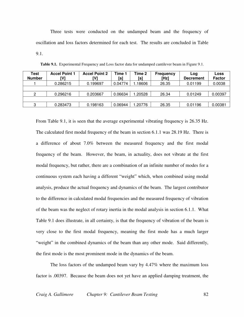
Craig A. Gallimore Chapter 9: Cantilever Beam Testing
82
Three tests were conducted on the undamped beam and the frequency of
oscillation and loss factors determined for each test. The results are concluded in Table
9.1.
Table 9.1. Experimental Frequency and Loss factor data for undamped cantilever beam in Figure 9.1.
Test Number
Accel Point 1 [V]
Accel Point 2 [V]
Time 1 [s]
Time 2 [s]
Frequency [Hz]
Log Decrement
Loss Factor
1 0.286215 0.199697 0.04774 1.18606 26.35 0.01199 0.0038
2 0.296216 0.203667 0.06634 1.20528 26.34 0.01249 0.00397
3 0.283473 0.198163 0.06944 1.20776 26.35 0.01196 0.00381
From Table 9.1, it is seen that the average experimental vibrating frequency is 26.35 Hz.
The calculated first modal frequency of the beam in section 6.1.1 was 28.19 Hz. There is
a difference of about 7.0% between the measured frequency and the first modal
frequency of the beam. However, the beam, in actuality, does not vibrate at the first
modal frequency, but rather, there are a combination of an infinite number of modes for a
continuous system each having a different “weight” which, when combined using modal
analysis, produce the actual frequency and dynamics of the beam. The largest contributor
to the difference in calculated modal frequencies and the measured frequency of vibration
of the beam was the neglect of rotary inertia in the modal analysis in section 6.1.1. What
Table 9.1 does illustrate, in all certainty, is that the frequency of vibration of the beam is
very close to the first modal frequency, meaning the first mode has a much larger
“weight” in the combined dynamics of the beam than any other mode. Said differently,
the first mode is the most prominent mode in the dynamics of the beam.
The loss factors of the undamped beam vary by 4.47% where the maximum loss
factor is .00397. Because the beam does not yet have an applied damping treatment, the

Craig A. Gallimore Chapter 9: Cantilever Beam Testing
83
loss factors are very low. Steel, as well as most other metals, have inherently low loss
factors because of their high stiffness and high modulus of elasticity. Having a high
stiffness makes them recover almost all of the loading energy after the load is removed.
Thus, once a damping treatment is applied and analyzed in the following sections, it was
expected that the damping and loss factors would greatly increase.
9.2 Dyad 601 Cantilever Beam Test Results
A strip of Dyad 601 was epoxied to the cantilever beam shown in Figure 9.1 and
constrained by a .96 mm thick aluminum layer. The cantilever beam was excited by hand
into transverse motion (pure pending) and allowed to vibrate freely for a period of 6
seconds. During this time, accelerometer data was being collected at 1600 Hz. A sample
plot for the acceleration data for Dyad 601 is shown in Figure 9.3.
Dyad 601 Cantilever Beam Acceleration Plot
-1.5
-1
-0.5
0
0.5
1
1.5
1.3
1.3
7
1.4
5
1.5
2
1.6
1.6
7
1.7
4
1.8
2
1.8
9
1.9
6
2.0
4
2.1
1
2.1
9
2.2
6
2.3
3
2.4
1
2.4
8
2.5
5
2.6
3
2.7
2.7
8
2.8
5
2.9
2 3
3.0
7
3.1
4
3.2
2
3.2
9
3.3
7
3.4
4
Time [s]
Vo
ltag
e [
V]
(99m
V/g
)
Figure 9.3. Acceleration data versus time for Dyad 610.
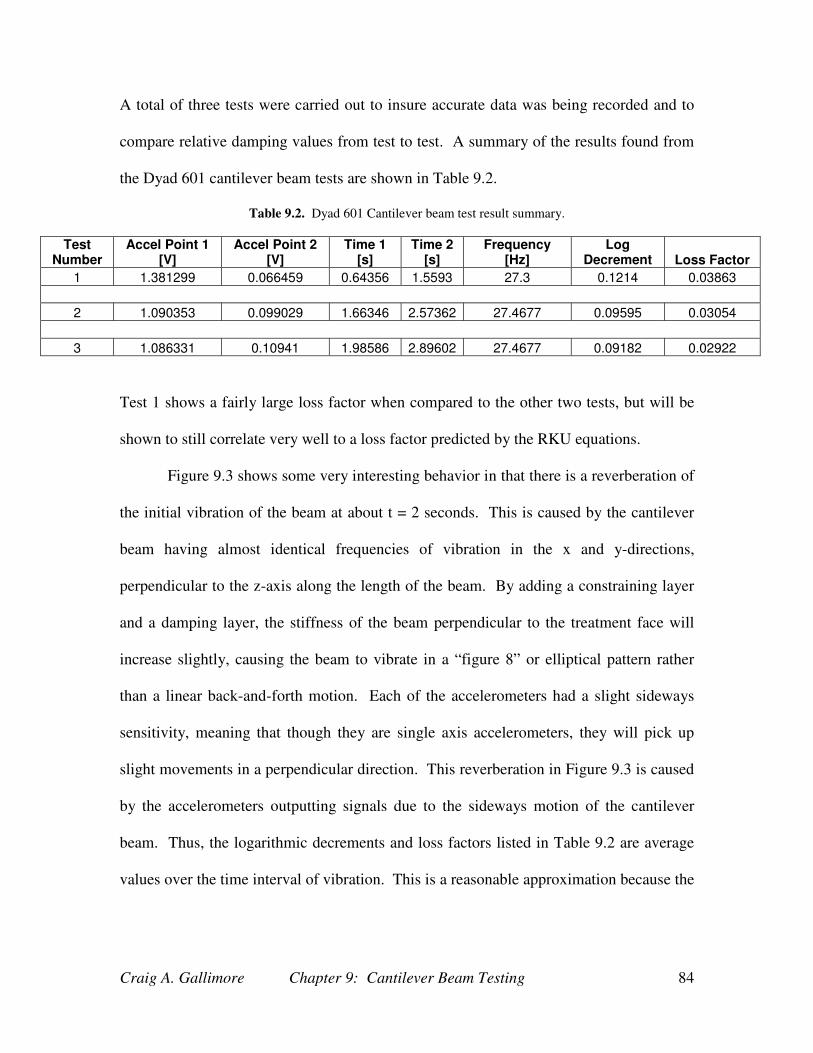
Craig A. Gallimore Chapter 9: Cantilever Beam Testing
84
A total of three tests were carried out to insure accurate data was being recorded and to
compare relative damping values from test to test. A summary of the results found from
the Dyad 601 cantilever beam tests are shown in Table 9.2.
Table 9.2. Dyad 601 Cantilever beam test result summary.
Test Number
Accel Point 1 [V]
Accel Point 2 [V]
Time 1 [s]
Time 2 [s]
Frequency [Hz]
Log Decrement Loss Factor
1 1.381299 0.066459 0.64356 1.5593 27.3 0.1214 0.03863
2 1.090353 0.099029 1.66346 2.57362 27.4677 0.09595 0.03054
3 1.086331 0.10941 1.98586 2.89602 27.4677 0.09182 0.02922
Test 1 shows a fairly large loss factor when compared to the other two tests, but will be
shown to still correlate very well to a loss factor predicted by the RKU equations.
Figure 9.3 shows some very interesting behavior in that there is a reverberation of
the initial vibration of the beam at about t = 2 seconds. This is caused by the cantilever
beam having almost identical frequencies of vibration in the x and y-directions,
perpendicular to the z-axis along the length of the beam. By adding a constraining layer
and a damping layer, the stiffness of the beam perpendicular to the treatment face will
increase slightly, causing the beam to vibrate in a “figure 8” or elliptical pattern rather
than a linear back-and-forth motion. Each of the accelerometers had a slight sideways
sensitivity, meaning that though they are single axis accelerometers, they will pick up
slight movements in a perpendicular direction. This reverberation in Figure 9.3 is caused
by the accelerometers outputting signals due to the sideways motion of the cantilever
beam. Thus, the logarithmic decrements and loss factors listed in Table 9.2 are average
values over the time interval of vibration. This is a reasonable approximation because the
Craig A. Gallimore Chapter 9: Cantilever Beam Testing
85
viscoelastic layer will damp out vibration in any direction, albeit delayed in this case by
the dynamics of the beam.
9.2.1 Dyad 601 Experimental and Theoretical Correlation
Per the composite loss factor for the cantilever beam given by the RKU prediction in
section 8.2, Table 9.2 shows very close correlation between experimental and theoretical
loss factor results. From Figure 8.2 given by the Dyad 601 RKU prediction, it was
estimated that a 1.31 mm Dyad 601 layer (as measured from the experimental cantilever
test) produced a composite loss factor of .0297 for a beam width of 9.53 mm and a
constraining layer of .96 mm by 9.53 mm. The average loss factor produced by the
cantilever tests was .0328, a value differing from the prediction by 9.47%. This average
loss factor for Dyad 601 is about 9.5 times the loss factor of the beam with no treatment.
By a treatment weight addition of about 12 grams, the loss factor of the beam was
increased almost 10 fold. Ultimately, the tested loss factor values prove that the RKU
equations produce very accurate predictions. However, the RKU equations are meant to
be an upper bound approximation, meaning they assume perfect energy conversion based
on the properties of a given viscoelastic material. Why, then, is the average
experimentally determined composite loss factor greater than the predicted value? The
material used to bond the Dyad to the beam and the constraining layer is a specially
formulated semi-flexible epoxy, which inherently carries small damping properties. In
fact, this epoxy, called B-Flex, was specifically formulated for the bonding of Dyad
materials to host structures to improve the damping of the Dyad polymer. Thus, there is
often a slight increase in damping because of the addition of several semi-flexible bond
layers which also promote damping.

Craig A. Gallimore Chapter 9: Cantilever Beam Testing
86
In general, the bonding layer should be of comparable stiffness to the host
structure, causing minimal slip between the host structure and damping material at the
bond interface. B-Flex epoxy is still very rigid compared to the Dyad material, but
because it was specifically formulated for Dyad materials, it was used in the beam tests.
Nevertheless, the experimental and theoretical results correlate extremely well for Dyad
601 with only about a 9.47% difference between theoretically determined loss factors and
those which were found experimentally.
9.3 Silicone 30A Cantilever Beam Test Results
A strip of silicone 30A rubber was sandwiched between the steel cantilever beam
and the aluminum constraining layer and excited to vibrate. During vibration,
accelerometer data was recorded and analyzed to find damping factors and loss factors of
each test. A total of three tests were conducted on the cantilever beam using silicone
30A. A sample plot of one of the tests is shown in Figure 9.4 and a summary of the
results from all three tests is provided in Table 9.3.
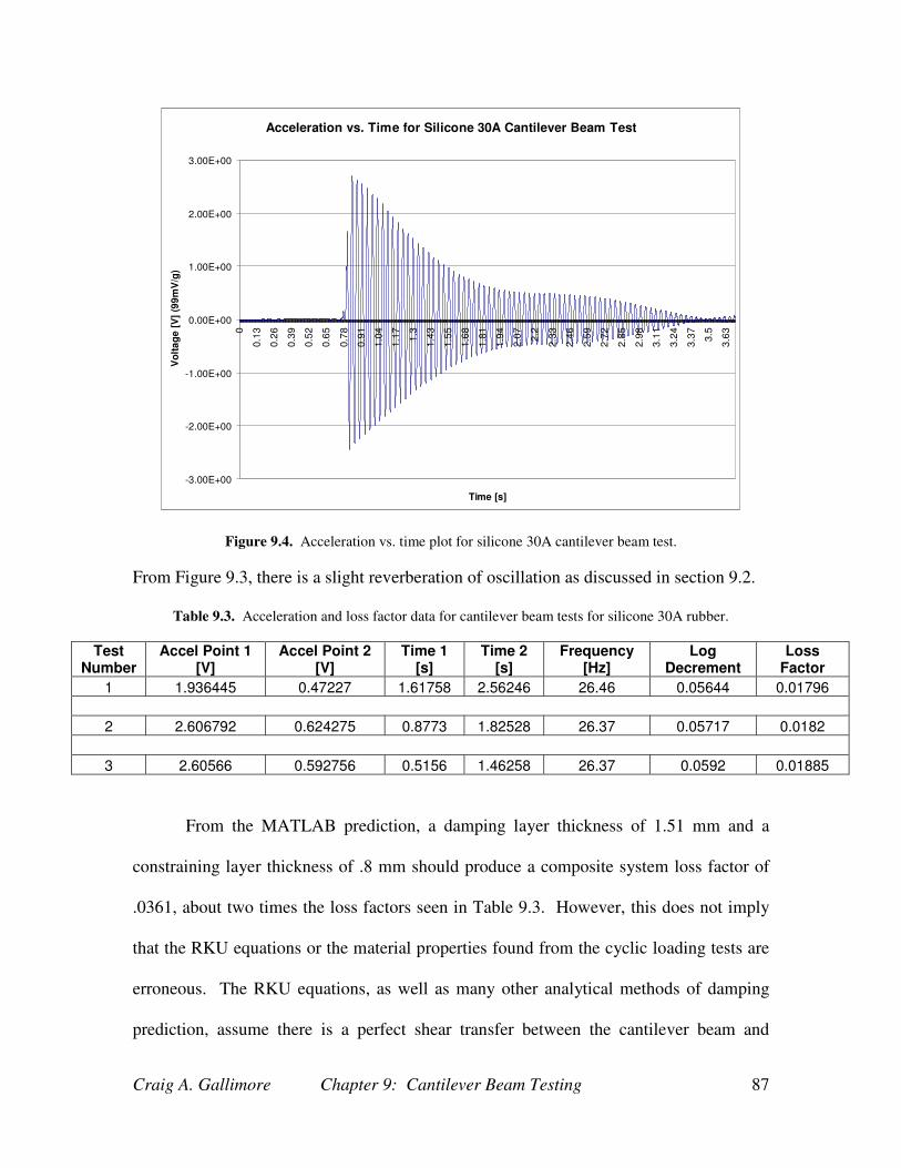
Craig A. Gallimore Chapter 9: Cantilever Beam Testing
87
Acceleration vs. Time for Silicone 30A Cantilever Beam Test
-3.00E+00
-2.00E+00
-1.00E+00
0.00E+00
1.00E+00
2.00E+00
3.00E+00
0
0.1
3
0.2
6
0.3
9
0.5
2
0.6
5
0.7
8
0.9
1
1.0
4
1.1
7
1.3
1.4
3
1.5
5
1.6
8
1.8
1
1.9
4
2.0
7
2.2
2.3
3
2.4
6
2.5
9
2.7
2
2.8
5
2.9
8
3.1
1
3.2
4
3.3
7
3.5
3.6
3
Time [s]
Vo
lta
ge
[V
] (9
9m
V/g
)
Figure 9.4. Acceleration vs. time plot for silicone 30A cantilever beam test.
From Figure 9.3, there is a slight reverberation of oscillation as discussed in section 9.2.
Table 9.3. Acceleration and loss factor data for cantilever beam tests for silicone 30A rubber.
Test Number
Accel Point 1 [V]
Accel Point 2 [V]
Time 1 [s]
Time 2 [s]
Frequency [Hz]
Log Decrement
Loss Factor
1 1.936445 0.47227 1.61758 2.56246 26.46 0.05644 0.01796
2 2.606792 0.624275 0.8773 1.82528 26.37 0.05717 0.0182
3 2.60566 0.592756 0.5156 1.46258 26.37 0.0592 0.01885
From the MATLAB prediction, a damping layer thickness of 1.51 mm and a
constraining layer thickness of .8 mm should produce a composite system loss factor of
.0361, about two times the loss factors seen in Table 9.3. However, this does not imply
that the RKU equations or the material properties found from the cyclic loading tests are
erroneous. The RKU equations, as well as many other analytical methods of damping
prediction, assume there is a perfect shear transfer between the cantilever beam and

Craig A. Gallimore Chapter 9: Cantilever Beam Testing
88
viscoelastic layer. This means that there is no slip at the bonding interfaces and that the
viscoelastic layer is shearing according to the dynamics of the beam. Additionally, the
bonding layer should be of comparable stiffness to the structural member to be damped,
meaning the adhesive should be fairly rigid and stiff. However, it was found during the
bonding of the silicone to the steel beam and aluminum constraining layer that silicone is
very difficult to bond to metals with a bonding layer having comparable stiffness to the
steel beam.
Several different grades of epoxy and cyanoacrylates were used and no sufficient
bond was formed. One and two part silicone adhesives and RTV’s were used with
limited success. The best bond between the silicone rubber sheet and the metal
components of the cantilever beam was made by using a general grade, clear RTV
silicone adhesive sealant most commonly used for bonding weather stripping in
automotive applications. However, this RTV adhesive, as well as almost all other RTV
adhesives, formed a very rubber-like bond, causing much of the shear normally found in
the viscoelastic layer to occur in the adhesive layer. Thus, the fundamental boundary
conditions found in the RKU equations are no longer satisfied because there is an
imitated slipping effect between the viscoelastic layer and the steel and aluminum faces it
was bonded to.
Phrased differently, if the bonding layer is very stiff and thin, the magnitude of
the vector from one point on the steel beam to its adjacent point on the viscoelastic layer
at the steel-silicone interface should not change during vibration. If the bonding layer is
very soft and rubbery, the magnitude of this vector will change. This concept is

Craig A. Gallimore Chapter 9: Cantilever Beam Testing
89
illustrated in Figure 9.5 for visualization. The thickness of the bonding layer is
exaggerated to illustrate the effect.
Figure 9.5. Deformation of rubbery bonding layer during bending.
With a rubbery bonding layer, the magnitude of this vector will change as the beam
vibrates, essentially causing a slip condition at the steel-silicone or aluminum silicone
interface. This rubbery bonding layer decreases the effectiveness of the silicone as a
damping material and results in the relatively low loss factors seen in Table 9.3.
9.4 Buna-N/Nitrile 40A Cantilever Beam Test Results
Cantilever beam tests similar to those carried out for Dyad 601 and silicone 30A
were also done using a nitrile 40A viscoelastic layer. The layer was measured to be 1.17
mm with a constraining layer thickness of .8 mm. The beam was excited to vibrate in
bending with a sample acceleration versus time plot show in Figure 9.6. The logarithmic
decrement was taken for each of three sets of acceleration data and the loss factor
calculated from each. The results are summarized in Table 9.4.
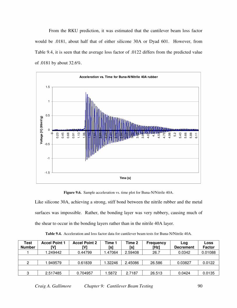
Craig A. Gallimore Chapter 9: Cantilever Beam Testing
90
From the RKU prediction, it was estimated that the cantilever beam loss factor
would be .0181, about half that of either silicone 30A or Dyad 601. However, from
Table 9.4, it is seen that the average loss factor of .0122 differs from the predicted value
of .0181 by about 32.6%.
Acceleration vs. Time for Buna-N/Nitrile 40A rubber
-1.5
-1
-0.5
0
0.5
1
1.5
0
0.2
3
0.4
5
0.6
8
0.9
1
1.1
3
1.3
6
1.5
8
1.8
1
2.0
4
2.2
6
2.4
9
2.7
2
2.9
4
3.1
7
3.3
9
3.6
2
3.8
5
4.0
7
4.3
4.5
3
4.7
5
4.9
8
5.2
5.4
3
5.6
6
5.8
8
6.1
1
Time [s]
Vo
lta
ge
[V
] (9
9m
V/g
)
Figure 9.6. Sample acceleration vs. time plot for Buna-N/Nitrile 40A.
Like silicone 30A, achieving a strong, stiff bond between the nitrile rubber and the metal
surfaces was impossible. Rather, the bonding layer was very rubbery, causing much of
the shear to occur in the bonding layers rather than in the nitrile 40A layer.
Table 9.4. Acceleration and loss factor data for cantilever beam tests for Buna-N/Nitrile 40A.
Test Number
Accel Point 1 [V]
Accel Point 2 [V]
Time 1 [s]
Time 2 [s]
Frequency [Hz]
Log Decrement
Loss Factor
1 1.249442 0.44799 1.47064 2.59408 26.7 0.0342 0.01088
2 1.949579 0.61839 1.32246 2.45086 26.586 0.03827 0.0122
3 2.517485 0.704957 1.5872 2.7187 26.513 0.0424 0.0135

Craig A. Gallimore Chapter 9: Cantilever Beam Testing
91
In order for accurate and representative loss factor values the nitrile rubber needed to be
securely bonded to the metal surfaces of the beam and constraining layer. The bond
inadequacies did not allow the nitrile 40A to damp out the vibration and oscillation of the
beam to its full potential.
9.5 Cantilever Beam Test Conclusions
The three best materials found from the RKU predictions, with material properties
found from cyclic loading tests, were bonded to a steel beam and constrained by a thin
piece of aluminum along the length of the beam. It was found from these tests that the
material properties of the damping layer were not always the most important factor in
damping out vibrations. Though silicone 30A and nitrile 40A showed higher loss factor
to shear modulus ratios than Dyad 601, they did not provide the expected damping per
the RKU prediction. The bond between the viscoelastic material and the adjacent metal
layers was determined to be the limiting factor in producing effective damping of the
beam. Additionally, because approximate loss factor and storage modulus data was
found per the cyclic loading tests, the discrepancy between the approximate complex
modulus values for the silicone 30A and nitrile 40A also contribute to the error seen
between RKU theoretical composite system loss factors and the system loss factors found
from experimental cantilever beam results. These approximate complex modulus values
vary from exact values by perhaps as much as 20% due to the assumptions made in
section 7.1, namely that the stress is uniform across the entire cross sectional area of the
test material and that the strain is uniform along the length of the test material.
Dyad 601, produced by Soundcoat Company, had a specially formulated epoxy to
help bond it to metal surfaces. This bond was found to be both strong and stiff,
Craig A. Gallimore Chapter 9: Cantilever Beam Testing
92
effectively eliminating any significant slip at the steel-Dyad and aluminum-Dyad
interfaces. This allowed the Dyad to shear properly and resulted in both significant
damping as well as the RKU prediction to be accurate. Both silicone and nitrile rubbers
could not be bonded to the metal substrates by a stiff enough adhesive. The rubbery
bonding layer of the silicone RTV did not allow the silicone or nitrile rubber to shear
properly, voiding their effectiveness as damping materials. Thus, despite the better
measured damping properties per the cyclic loading tests in section 7, Dyad 601 proved
to be the best damping material when experimentally tested on the cantilever beam.
In regards to a landing gear, bonding between the gear structural materials, in this
case 4140 steel, plays an even more significant role than bonding in the cantilever tests
because of the amplitude of deflection of the gear. The gear of interest in this report was
designed to deflect (change in height) several inches, much more than any tip deflection
in the cantilever tests. With higher deflection and higher strain in the steel gear, the
problem of delamination, or separation of the viscoelastic material from the gear
structure, becomes a looming problem. If the bonding layer is too stiff, it is subject to
crack and shear off of the gear material, which will render the damping layer useless.
However, if the bonding layer is too flexible, it will not transfer shear forces effectively
to the viscoelastic layer as seen with silicone 30A and nitrile 40A. Therefore, the B-flex
epoxy, a semi-flexible yet strong adhesive layer, is the most promising bonding material
for use in the gear. It showed excellent performance in the cantilever tests and is the
bonding material of choice in the application of a damping layer to the landing gear.
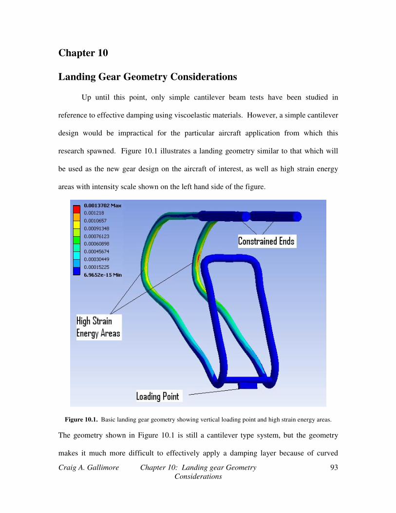
Craig A. Gallimore Chapter 10: Landing gear Geometry
Considerations
93
Chapter 10
Landing Gear Geometry Considerations
Up until this point, only simple cantilever beam tests have been studied in
reference to effective damping using viscoelastic materials. However, a simple cantilever
design would be impractical for the particular aircraft application from which this
research spawned. Figure 10.1 illustrates a landing geometry similar to that which will
be used as the new gear design on the aircraft of interest, as well as high strain energy
areas with intensity scale shown on the left hand side of the figure.
Figure 10.1. Basic landing gear geometry showing vertical loading point and high strain energy areas.
The geometry shown in Figure 10.1 is still a cantilever type system, but the geometry
makes it much more difficult to effectively apply a damping layer because of curved

Craig A. Gallimore Chapter 10: Landing gear Geometry
Considerations
94
surfaces and bend radii. Viscoelastic materials like the rubbers and specialty dampers
studied in this report are generally manufactured in the largest quantities as sheets. This
makes them easy to apply to flat surfaces without much alteration in the geometry of the
sheets. Additionally, constrained layer applications are even more difficult due to the
necessary manipulation and rigid bonding of a stiff constraining layer to a viscoelastic
material. Thus, a solution to this problem is proposed, although this solution is much
more difficult to accurately model for reasons which will be discussed.
Application of the relevant viscoelastic materials in section 8 providing
maximally effective damping would be difficult to apply if the material was kept in sheet-
like form. However, if these sheets were cut into long, narrow strips they could be
applied as a wrap. The application of the treatment would be slightly more tedious, but
the resultant damping very similar to a complete treatment. Also, if the constraining
layer were made thin enough, though this is undesirable (see section 8.5), it could also be
cut into thin strips and applied as a successful constraining layer, making the treatment
more effective than a free layer treatment.
The difficulty in modeling comes from the bonding layer, something that up until
this point is assumed very thin and flat. The bonding layer would cover the outer surface
of the gear host structure, but would also have a helical component bonding each section
of wrap to its adjacent sections. Additionally, this helical bonding layer inherently means
there would be gaps between each wrap, effectively making the treatment a partial
constrained layer treatment, something significantly more difficult to model than a simple
layer attached to the free surface of a cantilever beam. The helical component of the
bonding layer, however, is relatively negligible, but is nevertheless another component to
Craig A. Gallimore Chapter 10: Landing gear Geometry
Considerations
95
account for in an accurate damping prediction of the gear geometry. Recall that the
purpose of this report is to study and determine the best common damping materials
which could be used as a damping treatment for a small aircraft landing gear. The data
taken from these materials can then be extrapolated to other cantilever type systems
without the need to explicitly analyze the damping of the gear.
10.1 Round versus Square Material Geometry
The influence of a damping treatment applied to round versus square rod is two
fold. The first issue is a matter of mass and weight. Weight on an aircraft should be kept
to a minimum to maximize the flight time and aerodynamic efficiency of the aircraft.
Secondly, because damping via viscoelastic materials is dependent on shear, the distance
of a damping treatment to a neutral plane should be at a reasonable maximum, while
keeping any increases in mass and drag within proper limits.
Round rods have lower cross sectional area than square rods of the same
minimum cross section distance. Thus, round rods inherently have lower mass for the
same length and material of rod. They are, therefore, a better choice for a landing gear
material geometry than square rod. Additionally, from a design and manufacturing
perspective, round rod is easier to shape and form than square rod, making it cheaper and
faster to fabricate landing gear from round stock.
From a damping perspective, round rod does not offer the same amount of
damping per volume of damping treatment as square rod. A damping treatment need
only be applied to the flat faces of a square rod which are furthest away from the neutral
plane of the structural material during loading to achieve good damping. However,
damping material would need to be applied to the entire circumference of a round rod and

Craig A. Gallimore Chapter 10: Landing gear Geometry
Considerations
96
this does not even achieve the same level of damping as a square rod with less damping
material. More damping can be achieved with square rod using less material because
there is a larger surface area having larger bending strains than round rod. With round
rod, it is seen from Figure 10.1 that there is a thin strip of area, highlighted in red, having
large strains. This strip is the area of the rod furthest away and parallel to the neutral
plane during loading of the gear structure. Because there is a low surface area having
large strains, the viscoelastic treatment would have low effective area in which it could
utilize the strain energy of the area to dissipate energy. With a square rod however, if
bent and loaded in the same configuration, there is a much larger surface area having
large strains. Therefore it is not only the shear within the viscoelastic material, but also
the volume of material which has large shear within the damping layer. To increase the
volume of material with large shear, the treatment surface area should be increased and
applied to areas having the largest strain energies, promoting the largest possible shear
per volume within the viscoelastic layer.
Though square rod is initially more massive than round rod, round rod is a less
desirable material from a design perspective because of larger additions in weight from a
damping treatment and constraining layer and because it achieves less damping per
volume of material than square rod. The additions of weight by a damping material and
constraining layer to a round rod often nullify whatever weight advantage round rod had
over square rod. Additionally, more damping material is needlessly added to areas close
to the neutral plane of round rod, resulting in wasted material because the shear
deformation of the treatment layer becomes small closer to the neutral plane. As the
shear deformation decreases with the distance to the neutral plane, the material is no

Craig A. Gallimore Chapter 10: Landing gear Geometry
Considerations
97
longer effective at damping vibrations of the host structure because shear deformation is
the primary mechanism of damping in viscoelastic materials.
10.2 Landing Gear Design Conclusions
It has been shown that though round rod is initially less massive than square rod,
the damping of a round rod is much less for the same volume of damping treatment than
a square rod. The aircraft of interest in this report is approximately 400 lbs, so the gear
material was initially chosen to be 3/8” diameter steel rod. From Figure 10.1, a small
material diameter was chosen to minimize drag. The design process in determining
deflections and loads of the gear was facilitated by ANSYS finite element software.
The transition to square rod ultimately affects the design and dimension of the
gear as a whole. In bending, square rod has a larger flexural rigidity than round rod for
the same material and minimum cross section distance. The deflection and damping of
the gear were of primary concern, so to keep the deflection upon loading a constant, the
dimension of the square rod can be reduced to match that of the initial design using round
rod. Because the materials were kept the same, only the cross sectional area of the square
rod needed to be altered in order to produce a flexural rigidity matching that of the initial
design using round rod. Thus, a square rod having the same deflection of round rod can
be used where a much more efficient, weight saving damping treatment can be applied in
a much simpler fashion.
Craig A. Gallimore Chapter 11: Summary, Conclusions,
And Recommendations
97
Chapter 11
Summary, Conclusions, and Recommendations
The purpose of this report was to provide a basic knowledge of constrained layer
viscoelastic damping and to identify the best viscoelastic damping material to apply to a
landing gear while considering customer requirements such as cost, weight,
aerodynamics, environmental factors, and damping effectiveness. Eight viscoelastic
materials were chosen because of their low cost and durability. They were tested in an
ElectroPuls E1000 cyclic loading machine and an energy analysis was used to determine
their approximate elastic moduli and loss factors. These material parameters were then
used to formulate a damping prediction of a cantilever beam using the complex flexural
rigidity from the Ross, Kerwin, and Ungar analysis. The three best materials per the
RKU analysis were Silicone 30A, Buna-N/Nitrile 40A, and Dyad 601. These materials
were laminated to a cantilever beam and tested to experimentally determine the loss
factor of the beam and then compared to the RKU predictions. Dyad 601 showed the
best damping performance and correlation of experimental and theoretical loss factor
results. Silicone 30A and nitrile 40A rubbers showed sub-par performance due to the
difficulty in bonding these rubbers to metal surfaces.
In the application of these damping materials to the landing gear, these materials
are more efficiently bonded to flat surfaces. Thus, square rod is a choice material
geometry because less damping material can be bonded to the surfaces furthest away
from a neutral plane than for a round rod, where the damping material must be wrapped
around the entire circumference of the rod. Additionally, should round rod be bent into a
similar configuration as Figure 10.1, more damping material, and therefore more mass,
Craig A. Gallimore Chapter 11: Summary, Conclusions,
And Recommendations
98
must be added to the gear to achieve the same level of damping as a thinner damping
layer applied to the faces furthest from the neutral surface of a square rod.
The aerodynamic efficiency will decrease slightly in a transition from round rod
to square rod due to gear faces perpendicular to the free stream during flight. However,
during the cantilever tests, only one side of the cantilever beam was laminated with a
damping layer prior to testing. If both front and rear faces of a gear bent with square rod
are laminated with a treatment, a constraining layer having a cross section of a half circle
can be laminated to the viscoelastic treatment. This will increase weight by a small
margin, but will greatly reduce the drag of the gear and increase the loss factor due to a
thicker constraining layer.
11.1 Future Work
The first step in applying the conclusions found in this report is to fabricate and
test a landing gear with an applied damping treatment, preferably Dyad 601. The
structural member, steel rod, of the gear is cheap and relatively simple to fabricate. Thus,
several different gear structures can be made and a different damping treatment can be
applied to each, perhaps with a stand-off layer (Yellin, 1998), or spacer layer between the
metal and damping material to promote increased stresses within the layers, and therefore
better energy dissipation, within the damping layer. Each gear can then be fitted to the
aircraft and drop tested to isolate the best result.
The bonding of the silicone and nitrile rubbers was found to be the limiting factor
of damping in the cantilever beam tests. However, both silicone and nitrile rubbers are
easily molded or extruded around structural members. If a silicone or nitrile extrusion, or
even a mold encapsulating the metal of the gear and then filled with a pressurized flow of
Craig A. Gallimore Chapter 11: Summary, Conclusions,
And Recommendations
99
viscoelastic material, could be applied to the gear structure, much better damping may be
achieved. This would effectively eliminate any rubbery bonding layers with silicone or
nitrile rubbers and would also increase the interaction between the gear surfaces and the
damping layers.
As an alternative solution to using metal as the structural component in the gear,
fiber enhanced viscoelastic polymers could also be used (Alberts, 1995). A fiber
enhanced viscoelastic polymer is a series of thin, structural fibers like carbon or
fiberglass, encapsulated by a viscoelastic material. A series of strands having a
configuration similar to that of a frayed cable could be used as the basic structural
member of the gear. These strands could then be placed in a pressurized mold, having
the geometry of the gear in Figure 10.1, where a liquid viscoelastic material could then be
injected around the structural fibers encapsulating them in a viscoelastic matrix. This
would increase the contact surface area between the structural fibers and the damping
material as well as significantly reduce weight. Any loss in aerodynamic efficiency
would also be eliminated as the gear could take on the shape of the bare metal structure
of Figure 10.1.
Possible problems may arise in that the structural fibers would not be able to
accommodate loads on the extreme end of the landing gear design envelope.
Additionally, the damping material may need to be stiffer to help handle a small portion
of landing loads to assist the steel or composite fibers woven throughout the gear
geometry. Though the cost of fabricating this gear may be slightly higher than for a
metal gear, it is a viable solution for producing a gear with high damping, providing an

Craig A. Gallimore Chapter 11: Summary, Conclusions,
And Recommendations
100
effective, lower weight and more aerodynamic efficient material substitute for traditional
shock absorbers.

Craig A. Gallimore References
100
References
1) Alberts, T. E. and H. Xia. 1995. Design and Analysis of Fiber Enhanced
Viscoelastic Damping Polymers. Journal of Vibration and Acoustics. 117:
4:398-404.
2) Bagley, R. L. and P. J. Torvik. 1985. Fractional Calculus in the Transient
Analysis of Viscoelastically Damped Structures. AIAA Journal. 23: 6:918-925.
3) Birman, V. and L. W. Byrd. 2002. Analytical Evaluation of Damping in
Composite and Sandwich Structures. AIAA Journal. 40: 8: 1638-1643.
4) Buhariwala, K. J. and J. S. Hansen. 1988. Dynamics of Viscoelastic Structures.
AIAA Journal. 26: 2:220-227.
5) DiTaranto, R.A. 1965. Theory of vibratory bending for elastic and viscoelastic
layered finite length beams. Transactions of the ASME, Journal of Applied
Mechanics, 87, 881-886.
6) Hao, M. and M. D. Rao. 2005. Vibration and Damping Analysis of a Sandwich
Beam Containing a Viscoelastic Constraining Layer. Journal of Composite
Materials. 39: 18:1621-1643.
7) Jones, D. I. G. 2001. Handbook of Viscoelastic Vibration Damping. West
Sussex, England: John Wiley and Sons, LTD.
8) Kalyanasundaram, S., D.H. Allen, and R.A. Shapery. 1987. Dynamic Response
of a Timoshenko Beam. AIAA Journal. 559-567.
9) Kerwin, E.M. 1959. Damping of flexural waves by a constrained viscoelastic
layer. Journal of the Acoustical Society of America, 31(7), 952-962.
10) Lemerle, P. 2002. Measurement of the Viscoelastic Properties of Damping
Materials: Adaptation of the Wave Propagation Method to Tests Samples of
Short Length. Journal of Sound and Vibration. 250: 2:181-196.
11) Markley, D. W. and N. H. Madsen. 1988. Development of a Model for
Interfacial Damping. AIAA Journal. 1726-1732.
12) Mead, D.J., and Markus, S. 1969. The forced vibration of a three-layer, damped
sandwich beam with arbitrary boundary conditions. Journal of Sound and
Vibration. 10(2), 163-175.
Craig A. Gallimore References
101
13) Meirovitch, L. 2001. Fundamentals of Vibrations. New York, NY: McGraw
Hill.
14) Moreira, R.A.S. and J.D. Rodrigues. 2006. Partial Constrained Viscoelastic
Damping Treatment of Structures: A Modal Strain Energy Approach.
International Journal of Structural Stability and Dynamics. 6: 3:397-411.
15) Nashif, A. D., Jones, D. I. G., and J. P. Henderson. 1985. Vibration Damping.
Canada: John Wiley and Sons, Inc.
16) Rao, Y., V.K. Sadasiva, and Nakra, B.C. 1974. Vibrations of unsymmetrical
sandwich beams and plates with viscoelastic plates. Journal of Sound and
Vibration, 34(3), 309-326.
17) Ross, D., Ungar, E.E., Kerwin, E.M. Jr. 1959. Damping of plate flexural
vibrations by means of viscoelastic laminate. In ASME (Ed.). Structural
Damping (pp. 49-88). New York: ASME.
18) Saravanos, D.A. 1991. The Effects of Interply Damping Layers on the Dynamic
Response of Composite Structures. Proceedings, 32nd
Structures, Structural
Dynamics, and Materials Conference, 2363-2370. Baltimore, MD:
AIAA/ASME/ASCE/AHS/ASC.
19) Soundcoat Company. 2001. Soundcoat Dyad Material Data Sheet.
www.soundcoat.com.
20) Sun, C. T. and Y. P. Lu. 1995. Vibration Damping of Structural Elements.
Englewood Cliffs, NJ: Prentice Hall.
21) Torvik, P. J. 1996. Complex Rayleigh’s Quotient – A Means of Estimating Loss
Factors for Damped Systems. Proceedings, 37th
Structures, Structural Dynamics,
and Materials Conference and Exhibit, 1054-1063. Salt Lake City,
UT:AIAA/ASME/ASCE/AHS/ASC.
22) Yan, M.J., and Dowell, E.H. 1972. Governing equations for vibrating
constrained-layer damping of sandwich beams and plates. Transactions of the
ASME, Journal of Applied Mechanics, 94, 1041-1047.
23) Yellin, J. M. and I. Y. Shen. 1998. Analytical Model for a Passive Stand-Off
Layer Damping Treatment Applied to an Euler-Bernoulli Beam. Proceedings,
Smart Structures and Materials 1998: Passive Damping and Isolation. 349-357.
San Diego, CA: Society of Photographic Instrumentation Engineers.

Craig A. Gallimore Appendix A: MATLAB Programs
102
Appendix A: MATLAB Programs
Damping Predictions
function LF = RKU_Loss1(E_v, G_v, H_s, H_c, T_c)
%This function uses the RKU equations with inputs of elastic and shear
%modulus of the viscoelastic material, thickness of the structural member,
%thickness of the constraining layer, and width of the constraining layer
%and outputs composite system loss factor as a function of varying
%viscoelastic layer thickness.
L = .3557; %meters
E_s = 205E9; %Pascals
E_c = 68E9; %Pascals
omega_1 = 177.128; %rad/s
rho_s = 7800; %kg/m^3
i = 1;
k = 1;
LF = [];
for H_v = .0005:.0001:.009527
I_s = H_s^4/12; I_c = T_c*H_c^3/12;
zeta = sqrt(rho_s*H_s^2*omega_1^2*L^4/(E_s*I_s));
H31 = H_v + .5*(H_s+H_c);
H21 = .5*(H_s+H_v);
g = G_v*L^2/(E_c*H_v*H_c*zeta*sqrt(.9));
D = (E_v*H_v*(H21 - .5*H31) + g*(E_v*H_v*H21 + E_c*H_c*H31))/((E_s*H_s +
.5*E_v*H_v + g*(E_s*H_s + E_v*H_v + E_c*H_c)));
EI = E_s*H_s^3/12 + E_v*H_v^3/12 + E_c*H_c^3/12 - E_v*H_v^2/12*((H31 -
D)/(1+g))...
+E_s*H_s*D^2 + E_v*H_v*(H21-D)^2 + E_c*H_c*(H31 - D)^2 -
(.5*E_v*H_v*(H21 - D) + E_c*H_c*(H31 - D))*((H31 - D)/(1+g));
LF(i) = imag(EI)/real(EI);
i = i+1;
end

Craig A. Gallimore Appendix A: MATLAB Programs
103
H_v = [.0005:.0001:.009527];
plot(H_v, LF), xlabel('Viscoelastic layer thickness (m)'), ylabel('System Loss Factor')
title('Loss Factor vs. Viscoelastic Layer Thickness for First Modal Frequency (177.128
rad/s)')
Constrained Layer Effects
function LF = RKU_Loss_CL1(E_v, G_v, H_s, H_v, H_c, T_c)
%This function uses the RKU equations to predict changes in the loss factor
%of a composite beam system for varying constraining layer elastic modulus
%and thickness. Each section of code holds one variable (modulus or
%thickness) constant and varies the other.
L = .3557; %meters
E_s = 205E9; %Pascals
omega_1 = 177.128; %rad/s
rho_s = 7800; %kg/m^3
i = 1;
k = 1;
LF = [];
for E_c = 50000000000:1590000000:209000000000
I_s = H_s^4/12; I_c = T_c*H_c^3/12;
zeta = sqrt(rho_s*H_s^2*omega_1^2*L^4/(E_s*I_s));
H31 = H_v + .5*(H_s+H_c);
H21 = .5*(H_s+H_v);
g = G_v*L^2/(E_c*H_v*H_c*zeta*sqrt(.9));
D = (E_v*H_v*(H21 - .5*H31) + g*(E_v*H_v*H21 + E_c*H_c*H31))/((E_s*H_s +
.5*E_v*H_v + g*(E_s*H_s + E_v*H_v + E_c*H_c)));
EI = E_s*H_s^3/12 + E_v*H_v^3/12 + E_c*H_c^3/12 - E_v*H_v^2/12*((H31 -
D)/(1+g))...
+E_s*H_s*D^2 + E_v*H_v*(H21-D)^2 + E_c*H_c*(H31 - D)^2 -
(.5*E_v*H_v*(H21 - D) + E_c*H_c*(H31 - D))*((H31 - D)/(1+g));
LF1(i) = imag(EI)/real(EI);
i = i+1;

Craig A. Gallimore Appendix A: MATLAB Programs
104
end
E_c1 = [50000000000:1590000000:209000000000];
i = 1;
k = 1;
LF = [];
E_c = 68E9;
for H_c = .0005:.0001:.009527
I_s = H_s^4/12; I_c = T_c*H_c^3/12;
zeta = sqrt(rho_s*H_s^2*omega_1^2*L^4/(E_s*I_s));
H31 = H_v + .5*(H_s+H_c);
H21 = .5*(H_s+H_v);
g = G_v*L^2/(E_c*H_v*H_c*zeta*sqrt(.9));
D = (E_v*H_v*(H21 - .5*H31) + g*(E_v*H_v*H21 + E_c*H_c*H31))/((E_s*H_s +
.5*E_v*H_v + g*(E_s*H_s + E_v*H_v + E_c*H_c)));
EI = E_s*H_s^3/12 + E_v*H_v^3/12 + E_c*H_c^3/12 - E_v*H_v^2/12*((H31 -
D)/(1+g))...
+E_s*H_s*D^2 + E_v*H_v*(H21-D)^2 + E_c*H_c*(H31 - D)^2 -
(.5*E_v*H_v*(H21 - D) + E_c*H_c*(H31 - D))*((H31 - D)/(1+g));
LF(i) = imag(EI)/real(EI);
i = i+1;
end
H_c = [.0005:.0001:.009527];
LF1;
E_c1;
plot(H_c, LF, E_c1, LF1), xlabel('Constraining Layer Thickness (m)'), ylabel('System
Loss Factor')
title('Loss Factor vs. Constraining Layer Thickness for 1mm Damping Layer at 28.19
Hz')