Passive Spectrometer Design

8/7/2019 Passive Spectrometer Design

http://slidepdf.com/reader/full/passive-spectrometer-design 1/30

DESIGN AND CONSTRUCTION OF A PHOTODIODE-BASED PASSIVE

SPECTROMETER

by

Daniel T.S. Cook

PRINCIPAL SUPERVISORS:

Dr. William Heidbrink

Department of Physics and Astronomy

University of California, Irvine

Dr. Thomas Askew

Physics Department

Kalamazoo College

A paper submitted in partial fulfillment

Of the requirements for the degree of Bachelor of Arts at

Kalamazoo College

Fall Quarter, 2005



Contents

Acknowledgments iii

Abstract iv

I. Introduction 1

A. Plasma 1

B. Nuclear Fusion 1

C. Plasma Confinement 2

D. The Field-Reversed Configuration 3

E. The University of California, Irvine FRC Experiment 3

F. Plasma Diagnostics 4

G. Passive Spectroscopy, Line-Emission Spectroscopy 4

II. Background 5

A. FRC Theory 5

B. Spectroscopy Theory 7

C. Electron Temperature Determination 8

III. Spectrometer Design and Construction 9

A. Experimental Arrangement and Light Collection 10

B. Signal Generation and Amplification 10

C. Spectrometer Calibration 12

D. Spectral Line Ratio Measurements 15

E. Noise Reduction 16

IV. Results and Discussion 18

V. Conclusion 20

A. Relevant Spectral Line Information 23

B. Photodiode Calibration 23

C. Photodiode Characteristics 23

i



D. Filter Characteristics 23

E. Operational Amplifier Characteristics 23

F. Symbols 24

References 24

ii



Acknowledgments

Thank you to William Heidbrink for mentoring, advising, and assisting me throughout

my time on this project; Eusebio Garate and Thomas Askew for also advising me on this

project; Erik Trask and Wayne Harris for advice and assistance inside and outside the

scope of the project; Alan Van Drie for assistance with data collection; Princeton Plasma

Physics Laboratory and the US Department of Energy for supporting this project through

the National Undergraduate Fellowship Program in Plasma Physics and Fusion Energy

Sciences.

iii



Abstract

The use of passive spectroscopy to determine electron temperatures is well documented

and has the important benefit of being noninvasive. The use of line intensities in particular is

important because other spectrographic techniques, such as those based on Stark broadening

or Thompson scattering, can be difficult to employ in certain situations. Here, we present a

model for the estimation of electron temperature utilizing the ratio of emitted line intensities

in a plasma. Details of design and construction for a photodiode based spectrometer taking

advantage of this model are also presented, as well as details regarding data acquisition and

analysis using this spectrometer.

iv



I. INTRODUCTION

A. Plasma

Plasmas, the name given to ionized gases by Nobel laureate Irving Langmuir in the

early 1900’s, are thought to comprise the vast majority of matter in the known universe.

They exist naturally as interstellar clouds and solar wind, on the surface of stars, as the

earth’s ionosphere, around lightning, and in many other places [1]. Indeed, previously in the

history of the universe, all matter is thought to have been plasma [2]. Ever since Langmuir

founded the field of plasma physics through his research of tungsten-filament light bulbs,

the discipline has proved vital to further our understanding of the world around us.

Of more immediate interest to most however, are the man-made plasmas that are usefulto us everyday. From fluorescent lighting and neon signs, to semiconductor chip etching, to

arc welding, and even new plasma televisions, plasmas are becoming a part of our daily life.

And the potential for further exploitation of the unique properties of plasmas is such that

they are likely to become only more prevalent. Perhaps the most interesting, and possibly

the most useful, potential application of plasmas is to generate electrical power through

nuclear fusion.

B. Nuclear Fusion

Nuclear fusion occurs when two nucleii are joined together to produce a heavier nucleus,

generally with some excess energy. The energy required to produce fusion is extreme –

found in nature, for example, in the center of stars. At an energy level this high, neutral

atoms can ionize to become plasma. The process through which this takes place is well

understood. If it can be controlled, and the excess energy produced can be harnessed, it has

the potential to produce nearly boundless amounts of safe, non-polluting electrical power

for the future [3]. The reason that we are not yet using nuclear fusion as a power source is

because of the myriad challenging problems that exist with its actual implementation. The

large amounts of energy required are in fact attainable using our technology and resources.

A problem arises however, when having gathered this amount of energy one must then find

a way to channel it into the ions which are to be fused. After having overcome this hurdle,

which we only recently have, one must then direct the energy in such a way as to cause the

1



ions to collide and fuse. This last problem, the biggest that we still face, is the problem of

confinement.

C. Plasma Confinement

Since we are unable to direct ions well enough to cause collisions with a high probability,

the only way to achieve fusion is to energize the plasma, contain it the best we can, and

wait for the ions to collide on their own. Even if we were able to energize plasma to a

sufficient level for nuclear fusion in some sort of standard container, say a glass tube, steel

box, or some sort of specialized ceramic, the atoms on the wall in contact with the plasma

would very quickly also be ionized and turned into plasma. We are not even able to do this

however, because the energy lost by the plasma colliding with the walls would prevent us

from ever reaching the necessary excitation. In stars, the plasma is confined through the use

of immense gravitational fields. Unfortunately, this is not an option for us. On the bright

side, the ionized nature of plasma - which is what allows us to channel the energy into it

in the first place - presents us with a solution. The plasma can be confined magnetically,

and in so doing kept from coming in contact with the walls. Although the ionized nature of

plasma also brings with it other properties which make this type of confinement inherently

unstable, we have been able to counter the instabilities to some degree.

There have been many approaches to confining high energy plasmas, all of which are

understood to varying degrees. Most of these confinement schemes, such as the tokamak,

spherical torus, stellerator, spheromak, and others employ toroidal magnetic field geome-

tries of differing complexity. They generally require two main magnetic fields, one that acts

in a toroidal direction, and one that acts in a poloidal direction. Perhaps the most well

understood system is that of the tokamak, as is evidenced by the beginning of a recent

multinational, multi-billion dollar experiment called ITER located in France. This exper-

iment is designed to study and demonstrate the self-sustainability of a large-scale fusion

reactor. While the tokamak is the best understood confinement scheme, it has the drawback

of requiring great external energy input. The potential exists with some other sources for

a plasma which is self-organized to a greater degree, however these schemes tend to be less

well understood [4]. One promising such scheme is that of the field-reversed configuration.

2



FIG. 1: Sketch of magnetic fields in typical field-reversed configuration.

D. The Field-Reversed Configuration

In a field-reversed configuration (FRC), plasma confinement is achieved without the use

of a toroidal magnetic field. This is accomplished by using the magnetic properties of theplasma to freeze an initial magnetic field in a portion of the plasma, while reversing the

magnetic field surrounding it. This has the effect of creating areas of closed magnetic field

loops, as shown in Figure 1. This method has the advantages of having a large ratio of

particle pressure to magnetic field pressure (high β ) plasmas, providing an efficient way of

energizing the plasma, as well as having more self-organization than in other schemes [4].

Both of these aspects of FRCs cause them to require less initial energy input, as well as

less continuous energy input. As of yet FRCs have only been achieved for short durations,although these durations have been shown to be significantly longer than theory would

predict [4]. Unfortunately, this merely demonstrates the lack of understanding that exists

surrounding them, and more basic research must be conducted. This is the goal of the

University of California, Irvine FRC experiment (IFRC).

E. The University of California, Irvine FRC Experiment

The aim of IFRC is not to research nuclear fusion directly, but instead to investigate FRC

creation and confinement. As a result, it does not implement the standard method for FRC

creation, that of the Field Reversed Theta Pinch (FRTP). Instead, it uses a method known

as Coaxial Slow Source (CSS) formation, as described in Section II A. This method was

originally proposed by Phillips [5, 6], and first implemented at the University of Washington

[7]. This method is beneficial because conventional FRC techniques may be difficult to

implement in relatively large sizes [7].

3



F. Plasma Diagnostics

When conducting magnetic fusion research, one of the challenges that must be met is

that of gathering information about the plasma. Many methods have been developed to this

end, each with their own advantages and disadvantages. Perhaps the most common class

of methods is that of material probes, where physical objects are placed inside the plasma.

These objects can then be used to monitor the plasma itself, as is done with Langmuir probes,

or to monitor characteristics inside the plasma, such as measuring interior magnetic fields

with magnetic pickup coils. These methods have the advantages of being simple and well

understood, but have the disadvantages of being invasive and sometimes non-implementable

[8, 9].

Another class of diagnostic methods is active spectroscopy, where the plasma is probed by

exciting it in a specific way and observing the effects. Some examples of this are heavy-ion

beam probes and laser-induced flourescence, which inject heavy ions or energetic photons

into plasma. Similar to these methods are those such as microwave interferometry and

microwave reflectometry, where microwaves are launched into the plasma and their phase

shift and reflectance, respectively, are observed. These methods have the benefits of being

less invasive than material probes, as well as being implementable in some cases where

material probes are not. However, they are often very complicated and/ or expensive to

perform. Finally, there is a class of plasma diagnostics known as passive spectroscopy,

which will be the subject of this paper.

G. Passive Spectroscopy, Line-Emission Spectroscopy

Passive spectroscopy consists essentially of observing plasma externally without interfer-

ing with it. Some of the information that can be gathered regarding a plasma using thismethod are electron temperature, ion temperature, and electrical field information [10]. This

type of diagnostic has the advantage of being completely non-invasive, although it often sac-

rifices some degree of precision and resolution. Of particular interest in IFRC, as in many

experiments, is the measurement of electron temperature.

Although electron temperature can be measured in many ways, the approach that we

chose to adopt was that of line-emission spectroscopy. In line-emission spectroscopy, the

4



intensities of different spectral lines emitted from the plasma are compared, and these ratios

are used to calculate the temperature. Like other passive spectrographic techniques, good

temporal resolution can be achieved with this method, giving information on the thermal

evolution of the plasma throughout the experiment. Unfortunately, also like other passive

spectrographic techniques, it provides poor spatial resolution. We chose this method in

particular because other measurements, such as Stark broadening and Thompson scattering,

can not be employed for low energy plasma [8, 10, 11].

II. BACKGROUND

A. FRC Theory

As mentioned in section I D, the theory behind FRCs is still not complete [4]. Although

there has been some degree of success in forming FRCs, their high sensitivity to formation

and confinement parameters has caused experiments to remain largely based around trial

and error. Although some more recent improvements have aided in creating more control

and better behaved plasmas, the basic steps in FRC formation have remained much the

same.

The FRTP method for creating FRCs involves five basic stages, as is illustrated in Fig-ure 2. First, an initial ”bias” magnetic field is applied to contained gas, which is then ionized

to create plasma. The bias field induces an overarching flux which will be frozen into the

plasma throughout the lifespan of the FRC. The next stage is known as field reversal, where

the direction of external magnetic field is quickly reversed. During field reversal, as the

magnetic field initially decreases, the plasma expands toward the walls of the container.

Then, as the magnetic field increases in magnitude in the opposite direction, the flux of the

plasma induced by the bias field causes the plasma to be pushed toward the center of thecontainer and to lift off the wall. In the third stage, which begins directly after lift-off, the

plasma continues to implode radially. This causes the plasma to begin to heat. Oppositely

directed magnetic field lines near the ends of the plasma then pinch together, tear, and

reconnect. This reconnection begins the next stage, in which the reconnection causes an

axial contraction of the now self-contained plasma configuration, causing the plasma to heat

further. This continues until the final stage, in which equilibrium between all of the fields

5



FIG. 2: Typical steps in FRC Formation.

is reached and the FRC is completely formed [12].

In CSS formation, the magnetic fields required are generally induced by pulsing large cur-

rents through many separate toroidal coils surrounding the plasma. This has the advantages

of requiring smaller capacitor banks, which makes them more cost effective. It also allows

more control over the formation of the FRC, as well as allowing slow FRC formation. This

helps to study FRCs with better temporal resolution. In IFRC, the coils that are used are a

bias coil, a mirror coil, and a flux coil. The bias coil applies the initial magnetic field for the

FRC, which lasts throughout the experiment. The mirror coil applies a magnetic field on

the axial boundaries of the experiment which replace the field line tearing and reconnection

in a FRTP by containing the plasma using a magnetic mirror. This field also lasts through-

out the experiment. Unlike in an FRTP, both the bias coil and the mirror coil are fired in

vacuum. After these fields are reasonably established, pre-ionized plasma is injected axially

into the system. Once the plasma has had time to acquire the bias flux, the third and final

coil, the flux coil, is fired. The flux coil is fired at a higher power than the other two coils,

which results in a dominating magnetic field. It is fired in the opposite direction of the bias

coil so as to provide the field reversal necessary for FRC formation. The approximate timing

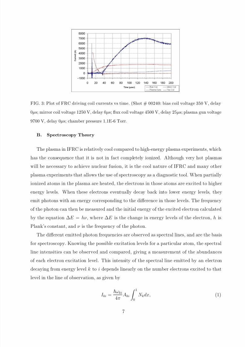
for the firing of these coils can be seen in Figure 3.

6



FIG. 3: Plot of FRC driving coil currents vs time. (Shot # 00240: bias coil voltage 350 V, delay

0µs; mirror coil voltage 1250 V, delay 0µs; flux coil voltage 4500 V, delay 25µs; plasma gun voltage

9700 V, delay 0µs; chamber pressure 1.1E-6 Torr.

B. Spectroscopy Theory

The plasma in IFRC is relatively cool compared to high-energy plasma experiments, which

has the consequence that it is not in fact completely ionized. Although very hot plasmas

will be necessary to achieve nuclear fusion, it is the cool nature of IFRC and many other

plasma experiments that allows the use of spectroscopy as a diagnostic tool. When partially

ionized atoms in the plasma are heated, the electrons in those atoms are excited to higher

energy levels. When these electrons eventually decay back into lower energy levels, they

emit photons with an energy corresponding to the difference in those levels. The frequency

of the photon can then be measured and the initial energy of the excited electron calculated

by the equation ∆E = hν , where ∆E is the change in energy levels of the electron, h is

Plank’s constant, and ν is the frequency of the photon.

The different emitted photon frequencies are observed as spectral lines, and are the basis

for spectroscopy. Knowing the possible excitation levels for a particular atom, the spectral

line intensities can be observed and compared, giving a measurement of the abundances

of each electron excitation level. This intensity of the spectral line emitted by an electron

decaying from energy level k to i depends linearly on the number electrons excited to that

level in the line of observation, as given by

I ki =ωki

4πAki

10

N kdx, (1)

7



where I ki is the spectral line intensity, is Plank’s constant, ωki is the frequency of the

spectral line, Aki is the transition probability for spontaneous emission per unit time, N k is

the population density of electrons in state k, and the integral is along the viewing sight-line

[8, 9].

C. Electron Temperature Determination

To calculate electron temperature from the intensities, we must make an assumption

about the distribution of energy in the system. We assume that the plasma is in partial

local thermodynamic equilibrium (PLTE), by which it is meant that the Saha and Boltzmann

thermal equilibrium relations provide good approximations. This assumption is possible

when free electron distributions are close to Maxwellian or Fermi distributions, and electron

densities are high enough that radiative rates are at least one order of magnitude smaller

than collisional rates [8, 13]. Applying PLTE to electron excitation populations, the ratio

in which the electrons decay to the same lower energy level is described by the equation

N kN i

=gkgi

exp

−E k −E ikT e

, (2)

where gk is the statistical weight – the total number of associated states – of the upper

energy level, gi is the statistical weight of the lower energy level, E k is the energy of the

upper level, E i is the energy of the lower level, k is Boltzmann’s constant, T e is the average

thermal energy of an electron in Kelvin, and so kT e is the plasma electron temperature

(average thermal energy) in electron volts.

If two different spectral lines are similarly observed, the ratio of the line intensities can

then be described by

I k1i1I k2i2

= Ak1i1gk1λk2i2Ak2i2gk2λk1i1

exp−E k1 −E k2

kT e

, (3)

[8, 9, 13, 14].

Now the electron temperature can be calculated by

8



kT e =− (E k1 −E k2)

ln

I k1i1I k2i2

Ak2i2gk2λk1i1Ak1i1gk1λk2i2

(4)

=−

(E k1−E k2)

ln

I k1i1I k2i2

/α

, (5)

where α is the line ratio coefficient:

α =Ak1i1gk1λk2i2Ak2i2gk2λk1i1

. (6)

The use of ratios is crucial because it only requires measurements of relative line intensi-

ties, as opposed to absolute line intensities. This has the result that if the two wavelengths

are observed in a similar fashion, factors such as population density and observed solid angle

can be ignored. This is beneficial because these factors may be unknown and/ or difficult

to measure.

Differentiating equation (3), we get

∆T eT e

=kT e

E k1 −E k2

∆(I k1i1/I k2i2)

(I k1i1/I k2i2). (7)

From this is is seen that if kT eE k1−E k2

becomes much larger than 1, errors in relative line inten-

sity measurements are amplified, which could result in large inaccuracies in the calculated

temperature [8, 14]. This is an effect that must be considered before deciding to implement

this method of plasma diagnostic for a particular experiment.

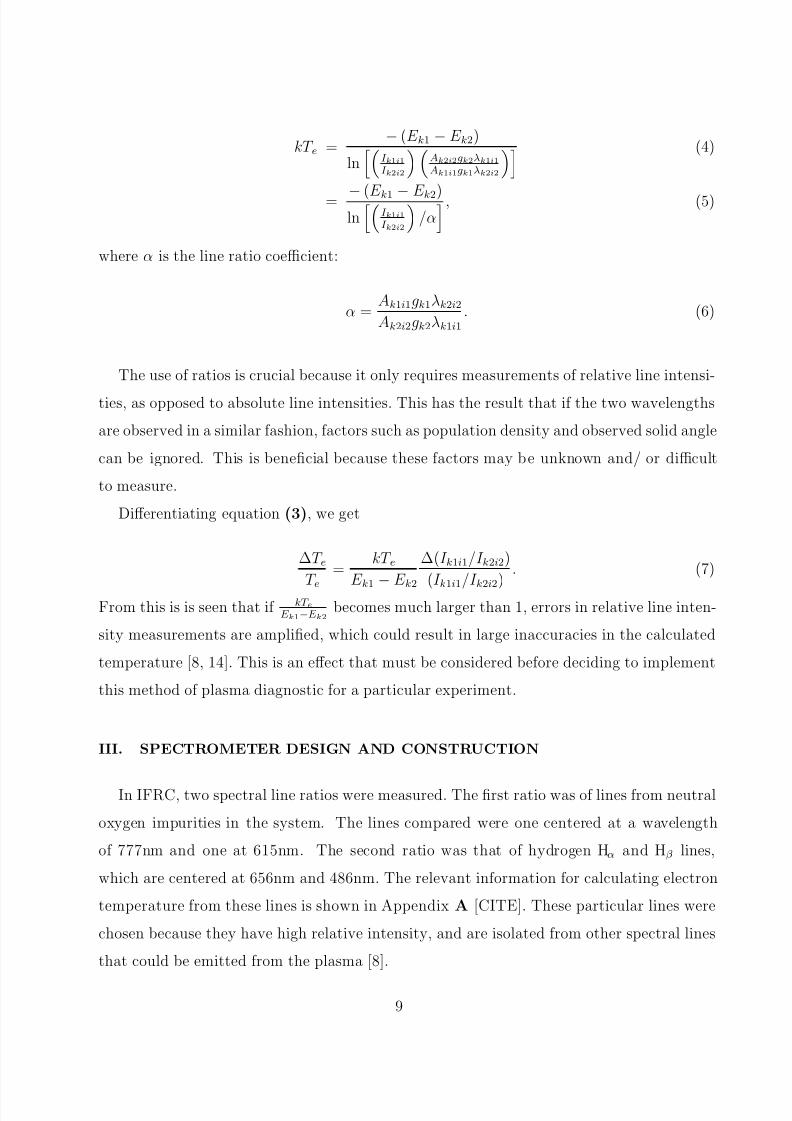
III. SPECTROMETER DESIGN AND CONSTRUCTION

In IFRC, two spectral line ratios were measured. The first ratio was of lines from neutral

oxygen impurities in the system. The lines compared were one centered at a wavelength

of 777nm and one at 615nm. The second ratio was that of hydrogen Hα and Hβ lines,

which are centered at 656nm and 486nm. The relevant information for calculating electron

temperature from these lines is shown in Appendix A [CITE]. These particular lines were

chosen because they have high relative intensity, and are isolated from other spectral lines

that could be emitted from the plasma [8].

9



FIG. 4: A schematic of the experimental set up for measuring electron temperature in IFRC using

spectrometer.

A. Experimental Arrangement and Light Collection

A schematic representation of the experimental set up for measuring electron temperature

in IFRC is shown in Figure 4.

The light emitted from the plasma was collected radially from the FRC through two

adjacent parallel aluminum pipes of diameter 0.25in and length 4in. These pipes were

placed directly against the viewing window of the FRC chamber. The pipe diameter was

chosen out of availability, and the length was chosen to balance the cross sectional viewed

area with the solid angle. The cross sectional viewed area needed to be small to eliminate

inaccuracies that could be caused by varying plasma density radially in the FRC. For this

reason also, the two pipes were aligned side-by-side axially along the FRC. The solid angle,

on the other hand, had to be as large as possible to allow enough light to be easily observed.

The collected light was then filtered through two 10nm full-width half-maximum narrow-

bandpass filters (TFI Technologies, Inc). The filters used were TFI 780-10 (780nm) and

610-10 (610nm) for the oxygen ratios, and TFI 660-10 (660nm) and 490-10 (490 nm) for the

hydrogen lines. The spectral characteristics of the specific filters is shown in Appendix D.

The collection pipes were placed inside an aluminum filter holder fabricated specially for the

spectrometer, and the filtered light was then directed through the same holder to a pair of

photodiodes.

B. Signal Generation and Amplification

The light through each filter was collected by a silicon photodiode. The particular photo-

diodes used (Hamamatsu Corp., S1227-33BR) were chosen for their high spectral response

10



FIG. 5: A schematic of the circuit used to provide a regulated reverse bias voltage to the photodi-

odes.

in the relevant range, as well as their fast rise time. Complete characteristics of these pho-

todiodes is shown in Appendix C. High spectral response was necessary to increase the

signal-to-noise ratio (SNR). The fast rise time was important to allow good temporal resolu-

tion throughout the FRC discharge, which in IFRC lasts between 50 and 100 microseconds.

It was estimated that an amplifier voltage gain near 100 was necessary to provide good

signal. A desired response frequency of 1MHz then necessitated the use of an amplifier with

a gain bandwidth product of approximately 100MHz. The operational amplifier, or op-amp,

chosen for its low noise and fast response time used was an LM6172, produced by National

Semiconductor. The LM6172 is a dual voltage feedback amplifier, the characteristics for

which are shown in Appendix E.

Each photodiode was then connected to an amplifying circuit, which was designed with

the desired characteristics (high amplification, low noise, and fast response time). The

photodiodes were reversed biased to allow operation in photo-conductive mode, which has

the advantage of faster and more linear response. The reverse biasing was accomplished

through the use of an Analog Devices ADP667 voltage regulator. The voltage regulator

was powered by one of two 9V batteries in the spectrometer, and the regulating circuit wasconstructed to provide a constant reverse bias voltage of approximately 2mV. This voltage

was chosen to balance the high linearity, high speed advantages of high reverse bias with

the low noise, high signal advantages of low reverse bias. Information regarding the voltage

regulating circuit is shown in Figure 5 and Table I.

The schematic for the amplifying circuit of one photodiode is shown in Figure 6 (note that

although the majority of the circuit components for each amplifying circuit were separate,

11



TABLE I: Voltage Regulating Circuit Characteristics

Set Resistor Output Resistor Output Capacitor Measured Output Voltage

Rset[Ω] Rout[Ω] C out[µF ] V out

473000 277400 18 1.925

the same op-amp could be used for both as it was dual channel). The photo-current from

each photodiode was passed through a load resistor of approximately 1000 ohms, which was

terminated to ground at a minimum distance. This provided current to voltage conversion,

and the voltage was passed directly into the non-inverting input of the op-amp, which was

powered by supply voltages of ±9V by the batteries. The inverting input of the op-amp

was also terminated to ground through approximately 1000 ohms at a minimum distance.

The output of the op-amp was then terminated to ground at 50 ohms and measured by

the oscilloscope, as well as being fed back into the inverting input through a resistance of

approximately 105 ohms. This circuit provided a theoretical V/A gain of approximately 105,

as is shown by

V o

I photo= R

l1 +

Rf

Rt (8)

= 1000

1 +

105

1000

≈ 105 (9)

where V o is the final output voltage, I photo is the photo-current from the photodiode, Rl is

the load resistor from the non-inverting input to ground, Rf is the feedback resistor to the

inverting input of the op-amp, and Rt is the terminating resistor from the inverting input

to ground. The actual gains were measured by driving the circuits with a known voltage

and recording the output voltage. The measured component characteristics, as well as themeasured gains are shown in Table II.

C. Spectrometer Calibration

To accurately calculate electron temperature, it is crucial that the relative line intensities

are accurately recorded. To insure this, all aspects of collection for each line intensity

measurement have to be calibrated against each other and taken into account. The different

12



FIG. 6: A schematic of the circuit used to amplify the photocurrent output from photodiodes.

TABLE II: Measured Spectrometer Circuit Characteristics

Circuit A Circuit B

Rl [Ω] 1041 1062

Rf [Ω] 100600 100600

Rt [Ω] 1043 1105

Rb [Ω] 9880 9860

Gainmeasured [V/A] 91439.18919 88978.37838

C 1 [µ F] 18

C 2 [nF] 0.3

C 3 [µ F] 18

C 4 [nF] 0.3

factors that had to be incorporated into the calibration were the photodiode efficiencies, the

different levels of circuit amplification, spectral response of the filters, and any geometric

differences resulting from gathering light from two separate pipes.

A schematic diagram of the experimental setup used to gather most of the calibration

information is shown in figure 7. In this setup the spectrometer was placed 10cm from

a tungsten bulb, which was used because it was adequate to provide light power over the

spectral regions necessary. The output voltages were then recorded for each photodiode with

no light reaching the diodes, unfiltered light reaching the diodes, and light passed through

each filter reaching the diodes. These values were compared to the light intensity at the

13



FIG. 7: A schematic of the experimental setup used to measure the relative photodiode efficiencies.

central wavelength as measured by a Newport Corp. Model 840 Optical Power Meter at 10cm

in the same scenarios. This setup was used because it provided a single calibration coefficient

(c1) that incorporated the photodiode efficiencies, circuit amplification, filter transmissions,

which was beneficial because the calculated electron temperature could depend sensitively

on all of these calibration factors. Although this method did not yield an accurate absolute

efficiency, it was sufficient because only a relative measurement was necessary. The results of

the calibration tests for both the oxygen and hydrogen filter sets are shown in Appendix B.Next, the geometric differences resulting from gathering light from two separate pipes

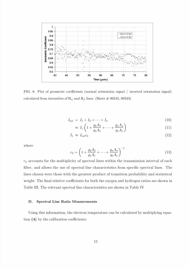
were measured (c2). This was found by first firing the FRC with the spectrometer attached

and in the standard orientation. The spectrometer was then inverted, and the FRC was

fired again. The geometric coefficient was then taken to be the quotients of the voltages

measured in these different orientations. A sample of the data from which this coefficient

was calculated is shown in Figure 8.

A final coefficient, c3, was required to account for the multiplicity of spectral lines withinthe transmission interval of each filter. This coefficient was calculated to allow the use of

values from one specific spectral line using a product of the atomic transition probability

and upper-energy-level statistical weight (see Appendix A):

14



FIG. 8: Plot of geometric coefficients (normal orientation signal / inverted orientation signal)

calculated from intensities of Hα and Hβ lines. (Shots # 00242, 00243)

I tot = I 1 + I 2 + · · · + I n (10)

≈ I 1

1 +

g2A2

g1A1

+ · · · +gnAn

g1A1

(11)

I 1 ≈ I totc3 (12)

where

c3 =

1 +

g2A2

g1A1

+ · · · +gnAn

g1A1

−1

(13)

c3 accounts for the multiplicity of spectral lines within the transmission interval of each

filter, and allows the use of spectral line characteristics from specific spectral lines. The

lines chosen were those with the greatest product of transition probability and statistical

weight. The final relative coefficients for both the oxygen and hydrogen ratios are shown in

Table III. The relevant spectral line characteristics are shown in Table IV

D. Spectral Line Ratio Measurements

Using this information, the electron temperature can be calculated by multiplying equa-

tion (4) by the calibration coefficients:

15



TABLE III: Relative Oxygen and Hydrogen Line Coefficients

Spectral Line Calibration Coefficient Geometric Coefficient Multiplicity Coefficient

Oxygen

780nm 1.118 1 0.467

615nm 1 1.414 0.525

Hydrogen

660nm 1.720 1 0.812

490nm 1 1.414 0.900

TABLE IV: Relevant Oxygen and Hydrogen Spectral Line Characterisitcs

Spectral Line λ [A] Aki[s−1] gk E k [eV]

Oxygen

780nm 777.194 36900000 7 10.741

615nm 615.818 7620000 9 12.754

Hydrogen

660nm 656.467 64650000 6 12.087

490nm 486.269 20620000 6 12.749

kT e =− (E k1 −E k2)

ln

I k1i1I k2i2

C α

, (14)

where C is the ratio of calibration coefficients:

C =c11c12c13

c21c22c23

(15)

E. Noise Reduction

To obtain usable data from the spectrometer, its SNR must be as high as possible. The

first aspect to be considered is photodiode noise. There are two main types of noise inherent

in the operation of a photodiode: thermal noise (or Johnson noise) and shot noise. The

thermal noise is associated with the shunt resistance of the photodiode, and is the same as

16



that present in all resistors. The shot noise is more specific to photodiodes, and is the result

of statistical fluctuations in photocurrent and darkcurrent. These are reduced by limiting

the operating temperature and reverse voltage bias on the photodiode, while maintaining

the maximum possible shunt resistance [15].

The other main types of noise inherent in the spectrometer result from the signal amplifi-

cation circuit. First, there is thermal noise associated with the op-amp and circuit resistors.

This is again reduced by limiting the operating temperature. Next, noise in op-amp supply

voltage can affect the degree of amplification of the signal. This noise is first reduced by

the use of batteries to provide DC power. This noise is then also rejected to some degree by

the op-amp itself. It can be further reduced by the use of voltage regulators on the input

voltage, and capacitors grounded at a minimum distance from the op-amp supply pins. All

of these methods are implemented in the IFRC spectrometer. Finally, external electromag-

netic (EM) noise can be coupled into the amplifying circuit. When coupled to the input or

feedback loops of the op-amp, this noise becomes amplified to the same degree as the signal.

For this reason, it is of the utmost importance to reduce this last noise as much as possible.

The first step in reducing external EM coupling is to reduce the size of all closed loops

inside the circuit as much as possible. This is accomplished by running any necessary wires

in twisted pairs, using the smallest components available, and connecting and terminating all

components at a minimum distance. This was also done with the IDE spectrometer. Next,

the entire spectrometer was enclosed in an aluminum box to provide a degree of shielding

from external EM noise. Upon firing IFRC however, large amounts of coupled noise were still

seen as ringing in the signal. An example of this noise is shown in Figure 9, in which all FRC

driving coils were fired, but no plasma was injected into the system. This was found to be

mainly the result of EM noise coupling to the output of the spectrometer from the crowbar

circuits used to limit the output voltage of the driving coils. This was reduced by moving the

oscilloscope to the maximum achievable distance from the crowbars, approximately 20 feet.

Further EM noise from the driving coils was reduced by using CAT-5 cable, which consists

wholly of twisted pairs, as the output cable from the spectrometer. Finally, large aluminum

plates were placed axially around the spectrometer for further shielding. Implementing these

measures reduced the noise considerably, as can be seen in Figure 10

17



FIG. 9: Plots of measured voltage vs time from spectrometer with no plasma, showing coupled

electromagnetic noise. (Shot # 00198)

FIG. 10: Plots of measured voltage vs time from spectrometer after noise reduction methods

implemented, showing final coupled electromagnetic noise. (Shot # 00216)

IV. RESULTS AND DISCUSSION

Voltages from both photodiode circuits were transmitted along the CAT-5 output cable

to an oscilloscope, which was set to run in single-shot mode to avoid accidental triggering.

The data recorded by the oscilloscope was then sent to a computer which compiled it along

with other data taken according to a computer program written by Alan Van Drie. The data

was recorded as a voltage, and then analyzed automatically at each time point according to

equation (14). The data was also analyzed manually using Microsoft Excel and Matlab. A

18



sample calculation using Hydrogen ratios for one specific time point is shown below (Shot

# 00245, 70 µsec):

C = c11c12c13c21c22c23

=1.720 ∗ 1 ∗ 1.232

1 ∗ 1.414 ∗ 1.111(16)

= 1.097 (17)

α =Ak1i1gk1λk2i2Ak2i2gk2λk1i1

= 64650000 ∗ 6 ∗ 486.26920620000 ∗ 6 ∗ 656.467

(18)

= 2.322 (19)

kT e =− (E k1 −E k2)

ln

I k1i1I k2i2

C α

=− (12.087 − 12.749)

ln−0.504−0.034

1.097

2.322 (20)

= 0.340 (21)

Unfortunately, the SNR of emitted oxygen lines in IFRC was initially too low to provide

provide good data regarding the evolution of the plasma electron temperature, and the

610nm filter became damaged before further testing could be done to remedy the problem.

The low SNR is likely the result of the relatively low temperature of the plasma, as well as

a large reduction of the line intensity as a result of the filtering. It is also possible that the

level of oxygen impurities in the plasma was less than expected, which could again lead to

low line intensities.

Hydrogen atoms and ions made up the bulk of the plasma, and so contributed the bulk of

the total emitted light. As a result, the SNR of the emitted hydrogen lines was much higher

than that of the oxygen lines, giving better data. There is a possibility that the observed

intensities in either of the hydrogen wavelengths could have been artificially inflated, and

hence the temperature made inaccurate, by the presence of carbon line in the same spectral

19



range. Estimates indicate however, that these carbon lines are lower in intensity by at least

an order of magnitude.

Figure 11 shows the results of shot # 00246. Plasma was injected into the system at

approximately10 µsec, at which point it was already slightly energized, and becomes further

energized due to the bias and mirror fields. Emitted light reached the photodiodes almost

immediately, however the SNR is too low to determine the electron temperature. Upon the

firing of the flux coil at approximately 35 µsec, the overarching magnetic field begins to

reverse. FRC was achieved at approximately 37.5 µsec and lasted until approximately130

µsec. After a slight delay, the electron temperature became easily discernible at approxi-

mately 50 µsec. This delay is likely the result of the specific spectral lines being observed:

Hα and Hβ are radiated from neutral Hydrogen atoms, so they must be heated secondarily

through collisional processes with free ions and electrons as opposed to being compressed or

heated directly by field reversal. During FRC, the electron temperature was observed to rise

from approximately 0.28 eV at approximately 50 µsec to a maximum of approximately 0.38

eV at approximately 90 µsec, and then decay to approximately 0.30 eV at approximately

110 µsec before the SNR becomes to great. The peak and subsequent decay are likely the

result of the plasma expanding as rotational or tilt instabilities began to break down the

FRC [6].

V. CONCLUSION

In this paper, we showed that the electron temperature of a low temperature FRC such as

IFRC can be estimated through spectral line emissions as measured by silicon photodiodes.

Although we were unable to use emissions from oxygen impurities in the system in my limited

time, we demonstrated the use of the Hα and Hβ line ratio to calculated this temperature.

Examples of the data that can be acquired were shown and analyzed. A passive spectrometer

constructed from silicon photodiodes along with amplifying circuits and narrow bandpass

filters is a feasible, low-cost diagnostic tool, and we presented one possible electrical and

mechanical design as well as the theoretical background. The main obstacle in constructing

and implementing this spectrometer was increasing the SNR in order to obtain useful data.

With a properly designed and constructed spectrometer as described above, the temporal

evolution of this temperature can be easily observed.

20



(a)

(b)

(c)

FIG. 11: Plots of (a) magnetic fields at radial distance from center R = 14, 44cm and axial distance

from chamber end Z = 10.7cm, (b) Hα and Hβ line intensity, and (c) corresponding calculated

plasma electron temperature vs time. (Shot # 00246: bias coil voltage 400 V, delay 0µs; mirror

coil voltage 1250 V, delay 0µs; flux coil voltage 4900 V, delay 25µs; plasma gun voltage 9500 V,

delay 0µs; chamber pressure 1.2E-6 Torr.)

21



TABLE V: Relevant Oxygen Spectral Lines

Wavelength Transition Probability Statistical Weights Relative Weight

(Lower, Upper)

λ [A] Aki[s−1] gi, gk

6046.23 1050000 3, 3 0.024091778

6046.44 1750000 5, 3 0.040152964

6046.49 350000 1, 3 0.008030593

6155.98 5720000 3, 3 0.13124283

6156.77 5080000 5, 7 0.271969407

6158.18 7620000 7, 9 0.524512428

7771.94 36900000 5, 7 0.466666667

7774.17 36900000 5, 5 0.333333333

7775.39 36900000 5, 3 0.2

TABLE VI: Oxygen Line Energies

Wavelength Lower Energy Level Upper Energy Level

λ [A] E i [eV] E k [eV]6046.23 10.988792 13.0388262

6046.44 10.988861 13.0388262

6046.49 10.98888 13.0388262

6155.98 10.740224 12.753715

6156.77 10.740475 12.753715

6158.18 10.740931 12.753715

7771.94 9.1460906 10.740931

7774.17 9.1460906 10.740475

7775.39 9.1460906 10.740224

22



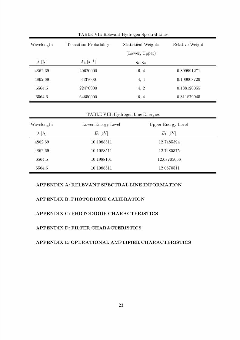
TABLE VII: Relevant Hydrogen Spectral Lines

Wavelength Transition Probability Statistical Weights Relative Weight

(Lower, Upper)

λ [A] Aki[s−1] gi, gk

4862.69 20620000 6, 4 0.899991271

4862.69 3437000 4, 4 0.100008729

6564.5 22470000 4, 2 0.188120055

6564.6 64650000 6, 4 0.811879945

TABLE VIII: Hydrogen Line Energies

Wavelength Lower Energy Level Upper Energy Level

λ [A] E i [eV] E k [eV]

4862.69 10.1988511 12.7485394

4862.69 10.1988511 12.7485375

6564.5 10.1988101 12.08705066

6564.6 10.1988511 12.0870511

APPENDIX A: RELEVANT SPECTRAL LINE INFORMATION

APPENDIX B: PHOTODIODE CALIBRATION

APPENDIX C: PHOTODIODE CHARACTERISTICS

APPENDIX D: FILTER CHARACTERISTICS

APPENDIX E: OPERATIONAL AMPLIFIER CHARACTERISTICS

23



APPENDIX F: SYMBOLS

c1 Relative spectrometer calibration coefficient 14

c2 Relative spectrometer geometric coefficient 14

c3 Spectral line multiplicity coefficient 14

CSS Coaxial Slow Source 3

E i Energy of an electron in energy level i 8

EM Electromagnetic 17

FRC Field-Reversed Configuration 3

FRTP Field Reversed Theta Pinch 3

gi Statistical weight of energy level i 8

h Planck’s Constant = 6.6262 × 10−

34 J s 7 Planck’s Constant = 1.0546 × 10−34 J s 8

i, k Specific electron energy levels 7

I ik Spectral line intensity emitted by an electron decaying from level i to k 8

I photo Photo-current from photodiode 12

IFRC University of California, Irvine FRC experiment 3

kT e Electron temperature (in electron volts) 8

N i Population density of electrons in state i 8Op-amp Operational Amplifier 11

Rf Feedback resistor 12

Rl Load resistor 12

Rt Terminating resistor 12

SNR Signal-To-Noise Ration 11

T e Electron temperature (in Kelvin) 8

V o Output voltage from Operational Amplifier 12α Line Ratio Coefficient 9

β Ratio of plasma particle pressure to magnetic field pressure 3

∆E Change in energy 7

ν Frequency 7

ω the frequency of an emitted spectral line 8

[1] R. Goldston and P. Rutherford, Introduction to plasma physics (Institute of Physics Publish-

ing, 1995). 24



[2] R. Fitzpatrick, Introduction to plasma physics (1998), course PHY380L, University of Texas

at Austin.

[3] The surprising benefits of creating a star (2001), for U.S. Department of Energy, Offices of

Fusion Energy Sciences.[4] M. Brown, Alternate concepts, Lecture (2005), for National Undergraduate Fellowship Pro-

gram in Plasma Physics and Fusion Engineering.

[5] J. Phillips, Tech. Rep. LA-8711-P, Los Alamos National Laboratory (1981).

[6] M. Tuszewski, Nuclear Fusion 28, 2033 (1988).

[7] Z. Pietrzyk, G. Vlases, R. Brooks, K. Hahn, and R. Raman, Nuclear Fusion 27, 1478 (1987).

[8] O. Garate, for TriAlpha Energy Corporation, Irvine CA.

[9] R. McWhirter, Spectral intensities (Academic Press, 1965), chap. 5.

[10] J. Foley, Plasma diagnostics, Lecture (2005), for National Undergraduate Fellowship Program

in Plasma Physics and Fusion Engineering.

[11] I. Hutchinson, Principles of plasma diagnostics (Cambridge University Press, 1987).

[12] A. Hoffman, R. Milroy, J. Slough, and L. Steinhauer, Fusion Technology 9, 48 (1986).

[13] H. Griem, Principles of plasma spectroscopy (Cambridge University Press, 1997).

[14] Z. Andreic, Ph.D. thesis, University of Zagreb (1993).

[15] Photodiode Technical Information , Hamamatsu Corporation (????).

25

Passive Spectrometer Design

Documents

Transcript of Passive Spectrometer Design