Passive, Privacy-preserving Real-time Counting ofUnmodified Smartphones via ZigBee Interference

Roman Lim, Marco Zimmerling, Lothar ThieleComputer Engineering and Networks Laboratory

ETH Zurich, Switzerland{lim, zimmerling, thiele}@tik.ee.ethz.ch

Abstract—The continuing proliferation of smartphones makesthem an effective means to monitor the number of people withinan area, for example, to gain insights into customer engagement inretail and to enable an intelligent traffic system in a city. However,current approaches to obtain this information are either invasiveas they require to continuously run a dedicated smartphone app,or they compromise users’ privacy by sniffing the MAC addressesof their smartphones. As a consequence, lawyers, authorities, andthe population are very skeptical toward adopting such innovativesystems. We present DEVCNT, the first system that counts in real-time the number of Wi-Fi enabled smartphones in a non-invasivemanner while preserving by design the privacy of the smartphoneusers. This paper details how DEVCNT detects active Wi-Fi scansperformed by smartphones on a ZigBee device, and how DEVCNTuses the number of detected scans to estimate the number of Wi-Fi enabled smartphones. Results from controlled and real-worldexperiments show that DEVCNT: (i) detects more than 99 % ofactive Wi-Fi scans even under interference from multiple wirelesstechnologies, (ii) achieves up to 91 % accuracy in the estimatedsmartphone counts, and (iii) provides meaningful estimates in areal test run involving hundreds of Wi-Fi transmitters.

I. INTRODUCTIONSmartphones are an integral part of our daily lives, and will

be even more so in the future. Ericsson forecasts 5.6 billionsmartphones around the world in 2019, accounting for 60 % ofall mobile subscriptions [8]. This proliferation is intriguing asit opens up the possibility to exploit smartphones for collectingstatistically significant amounts of data about the way peoplebehave and interact [3]. In addition, nowadays almost everysmartphone has Wi-Fi built in. Due to ever-increasing mobiledata traffic [8], users activate Wi-Fi on their smartphones to getfast and cheap connectivity to a Wi-Fi network whenever pos-sible. To discover these offloading opportunities, smartphonesactively scan for Wi-Fi access points (APs) by periodicallysending out probe request frames, or probes for short.Motivation. We seek to leverage the high proliferation of Wi-Fi enabled smartphones to determine their numbers in real-timebased on the probes they emit. Given the high penetration ofsmartphones across the general population, such counts are ofgreat value in numerous applications. For example, they can beused to estimate the density of a crowd, which is an importantfeature in crowd management [11] to prevent disasters likethe 2010 Love Parade stampede that killed 18 people [25]; inretail, they provide insights into customer engagement and helpimprove in-store sales [5]; and in a city, information about thenumber of pedestrians, cyclists, and motorists using particularroad segments at any given time enables an intelligent transportsystem where traffic lights adapt to reduce travel times [24].

Prior to the advent of the smartphone, video surveillanceand image processing have been used to estimate the number of

people in an area [13]. These solutions, however, need special-purpose powered equipment and impact privacy. Today, analternative solution is to encourage people to run an applicationon their smartphones that periodically sends the GPS locationto a server [27]. While here users can opt out at any time, thisapproach is invasive in that it alters the smartphone software,and works only outdoors where GPS reception is possible.

A non-invasive approach is to use existing Wi-Fi APs or todeploy dedicated Wi-Fi monitors to estimate people count bysniffing the unique MAC addresses of their smartphones, whichare contained in clear text in every probe [5], [20]. From aprivacy perspective, this is even worse than video surveillancebecause the owner, which can be unequivocally identified fromthe MAC address, has no means to notice that she is beingtracked. Thus, lawyers, authorities, and the population take askeptical position despite the use of anonymization techniquessuch as MAC address hashing. This could be witnessed, forexample, by a public outcry and eventual ban of such a systemin the City of London [23], and unclear current law preventingthe deployment of a smart traffic system in Copenhagen [24].Contribution. To address these issues, we introduce DEVCNT,a system providing real-time estimates on the number of Wi-Fienabled smartphones within an area in a non-invasive manner.DEVCNT preserves by design the privacy of smartphone users,thus overcoming the concerns associated with prior approachesand fostering the rapid deployment of innovative applications.

To this end, DEVCNT takes advantage of cross-technologyinterference in the 2.4 GHz band. As described in Sec. II, theIEEE 802.11 standard prescribes that an active scan shouldinvolve sending a probe on each Wi-Fi channel. Since each Wi-Fi channel overlaps with at least one ZigBee channel, a ZigBeedevice can perceive a probe transmission as a short increasein the received signal energy. DEVCNT uses one or multiplebattery-powered ZigBee devices to flexibly cover large areas.Every device periodically reports the number of active Wi-Fiscans it has seen to a sink. Based on the received scan counts,DEVCNT estimates at the sink the number of Wi-Fi enabledsmartphones within the range of each ZigBee device.1

DEVCNT works both indoors and outdoors, and provides anew estimate every few seconds. DEVCNT is non-invasive andfully passive in that it neither modifies the software running onthe smartphones, nor does it externally affect the smartphones’operation (as done in [20]). Because it is technically impossiblefor a ZigBee receiver to demodulate Wi-Fi frames, DEVCNTcannot track individual smartphones nor identify their owners.

1Since this paper deals primarily with the physical and media access layersof IEEE 802.15.4 and IEEE 802.11, we do not discern between these standardsand the respective industrial alliances ZigBee and Wi-Fi.

Finally, by using low-power wireless battery-powered devices,DEVCNT reduces costs and increases flexibility during systeminstallation, maintenance, and removal compared with previoussolutions that use video surveillance or Wi-Fi monitors.

Achieving these favorable properties while providing accu-rate smartphone counts is challenging for at least three reasons:• Amplitude and time resolution of received signal strength

(RSSI) information on a ZigBee receiver is coarse-grained.DEVCNT must therefore cope with inaccuracies when char-acterizing Wi-Fi transmissions by their length and signalstrength, which are the only features DEVCNT is left withto detect scans on a device that cannot demodulate Wi-Fi.

• DEVCNT cannot differentiate between individual smart-phones because it cannot not see their (unique) MACaddresses, probes from different smartphones may have thesame length, and RSSI is a poor classifier due to mobilityand multipath fading. While this preserves privacy, it alsomakes counting Wi-Fi enabled smartphones a difficult task.

• Sending all RSSI samples to a central sink for processing isprohibitive due to the limited bandwidth. Thus, as detailedin Sec. III, DEVCNT performs most of the required process-ing on the ZigBee devices. This, in turn, implies that eachZigBee device needs to multiplex its single microcontrollerunit (MCU) between three tasks: (i) reading RSSI samples,(ii) processing samples to detect and count scans, and (iii)sending scan counts to the sink. DEVCNT must temporallydecouple (i) and (ii) from (iii) synchronously on all devicesto avoid distorting the smartphone count estimations due toself-interference, while simultaneously reducing the timeneeded for (iii) to have more time available for (i).As discussed in Secs. IV and V, we tackle these challenges

by designing novel signal processing, feature extraction, andclassification algorithms. Given that these algorithms need toexecute in real-time on devices with severely limited memoryand compute power, our algorithms strike a balance betweenfeasibility and optimality. The key insight we use to countsmartphones without being able to distinguish them is that theactive Wi-Fi scanning rate of a sizable population of smart-phones follows a specific and typically narrow distribution. Toenable temporal decoupling and fast all-to-one data collection,we use Glossy [9] to accurately time-synchronize the ZigBeedevices and Chaos [16] as efficient communication support.

To demonstrate the feasibility of our design, we implementa DEVCNT prototype on the TelosB [21] platform. In Sec. VII,we evaluate DEVCNT in controlled experiments with up to 31smartphones from 4 different vendors running iOS or Android,and during a real-world test run in a large lecture hall withmore than 100 students. Our results show the following:• DEVCNT accurately detects more than 99 % of Wi-Fi scans

despite realistic interference from Bluetooth, ZigBee, andWi-Fi traffic, the latter including TCP and UDP streams.

• DEVCNT detects scans with an accuracy above 90 % evenon ZigBee devices that are 50 m away from the phone.

• In a controlled experiment where the precise ground truth isavailable, DEVCNT estimates the number of Wi-Fi enabledsmartphones with accuracies of up to 91 %.

• In a real-world test run where the ground truth is extremelydifficult to obtain, DEVCNT’s processing pipeline sustainssignals from hundreds of Wi-Fi transmitters, thus providingmeaningful smartphone counts that match the expectations.Sec. VIII discusses trade-offs and limitations of DEVCNT,

Sec. IX reviews related work, and Sec. X concludes the paper.

1 2.412

2 2.417

3 2.422

4 2.427

5 2.432

6 2.437

7 2.442

8 2.447

9 2.452

10 2.457

11 2.462

12 2.467

13 2.472

14 2.484

11 2.405

12 2.410

1 2.412

13 2.415

14 2.420

15 2.425

16 2.430

17 2.435

18 2.440

19 2.445

20 2.450

21 2.455

22 2.460

23 2.465

24 2.470

25 2.475

26 2.480

Wi-Fi Channel Center Freq. (GHz)

Channel Center Freq. (GHz) ZigBee

Figure 1. IEEE 802.11b/g (Wi-Fi) and IEEE 802.15.4 (ZigBee) channels inthe 2.4 GHz industrial, scientific and medical (ISM) band.

II. BACKGROUND AND TERMINOLOGYDEVCNT takes advantage of cross-technology interference

between Wi-Fi and ZigBee in the 2.4 GHz band. IEEE 802.11defines in total 14 channels, as shown in Fig. 1. Each channelis 22 MHz wide and the center frequencies range from 2.412to 2.484 GHz. Channel 14 is forbidden in most parts of theworld, and channels 12 and 13 are typically not used in NorthAmerica due to FCC regulations. IEEE 802.15.4 defines intotal 16 channels with a bandwidth of 2 MHz each and centerfrequencies between 2.405 and 2.480 GHz. Thus, ZigBee andWi-Fi can interfere when operating in overlapping channels.

While often regarded as a major impediment to the perfor-mance of ZigBee networks [17], DEVCNT takes advantage ofthis kind of interference. It uses received signal strength (RSSI)information available on commodity ZigBee devices to detectan interfering Wi-Fi transmission from a short-lived increase inthe RSSI. According to the IEEE 802.15.4 standard, the RSSIvalue is an average over the last 8 symbol periods (128µs),and is typically updated on a per symbol basis, that is, every16µs. Furthermore, many ZigBee radios allow to adjust theiroperating frequency with a certain granularity (e.g., 1 MHz onthe CC2420 radio [22]). As explained in Sec. VI, we use thisfeature in DEVCNT to best align the operating frequency of theZigBee devices with the center frequency of a Wi-Fi channel.

The majority of Wi-Fi networks operates in infrastructuremode, where access points (APs) manage all communications.A client, such as a laptop or a smartphone, needs to associatewith an AP before it can use any network services. TheIEEE 802.11 standard defines, among other things, a processcalled active scanning, whereby a client sends probe requestframes (probes) to discover an AP. The standard prescribesthat an active scan should involve broadcasting a probe oneach channel, awaiting and processing possible responses fromAPs in between. Nevertheless, no further detailed specificationof active scanning is provided in the IEEE 802.11 standard.As a result, different Wi-Fi drivers implement active scanningslightly differently. For example, we noticed that many driverssend multiple probes (mostly two) on each channel, as op-posed to just one probe. Smartphones perform active scanningperiodically every few tens of seconds [10], depending on theoperating system and the current operating mode (e.g., whetherthe smartphone is actively used or in standby mode).

Although there is also a passive scanning process foreseenin the IEEE 802.11 standard, where clients passively listenfor beacon frames from APs, mobile devices mostly rely onactive scanning because it is faster. Typically, APs announcetheir presence by sending a beacon frame every 102.4 ms. Aclient must listen for at least that period on every channelto finish a passive scan, whereas probe requests are usuallyhandled within a much shorter time. In the remainder of thispaper, we use the term scan to refer to active scans.

An IEEE 802.11b/g frame is preceded by a preamble thatis at least 96µs long. This is above the 16µs symbol period of

Detect and count active scansSignal extraction Feature extraction

Smartphone countestimationRSSI

samples

On ZigBee devices On base station

Signal clustering ClassificationSec. V-A Sec. V-B Sec. V-C Sec. V-D Sec. IV

Figure 2. High-level view of DEVCNT. A multi-hop low-power wireless network of ZigBee devices continuously samples the received signal strength (RSSI),and uses a novel signal processing pipeline to detect and count active Wi-Fi scans performed by smartphones. Based on the scan counts periodically reportedby the ZigBee devices, DEVCNT estimates on a base station the number of Wi-Fi enabled smartphones within the reception range of each ZigBee device.

time

detection windows

counting window

reporting interval

…  

RSSI & processing communication

Figure 3. Illustration of how the activities of RSSI sampling, processing,and communication evolve over time in DEVCNT. To avoid negative self-interference effects, RSSI sampling and processing are temporally decoupledfrom communication. The reporting interval determines the timeliness ofsmartphone counting in DEVCNT, which is on the order of a few seconds.

IEEE 802.15.4, so Wi-Fi frames are, in principle, detectablefrom the RSSI samples of a ZigBee radio. After the preamble,a Wi-Fi probe contains in unencrypted form the client’s MACaddress, the broadcast address or the SSID of a known Wi-Fi network of up to 32 bytes, the data rates supported by theclient, and other (e.g., vendor-specific) information.

III. DEVCNT OVERVIEWWe present DEVCNT, the first system that provides real-

time estimates on the number of Wi-Fi enabled smartphonesin an area in a fully passive and non-invasive manner withoutrevealing the identity or movement profile of smartphone users.

DEVCNT counts the number of Wi-Fi enabled smartphonesbased on the probes they send while actively scanning fornearby Wi-Fi APs. Instead of directly eavesdropping on probesusing a Wi-Fi capable receiver, DEVCNT detects probes indi-rectly via their interference patterns at a ZigBee receiver. SinceZigBee radios cannot demodulate Wi-Fi probes, DEVCNT doesnot see the unique MAC addresses contained therein and henceis unable to identify individual phones. As a result, DEVCNTpreserves by design the privacy of the smartphone users, whichsharply differentiates DEVCNT from prior art [5], [13], [20].Moreover, DEVCNT is fully passive and non-invasive: It doesnot influence a smartphone’s normal operation, for example,by soliciting more probe transmissions [20], nor does it requiremodifications to the smartphones themselves, such as installingand running a dedicated application [27].

Fig. 2 provides a high-level view of DEVCNT, while Fig. 3illustrates how the different activities in DEVCNT evolve overtime. DEVCNT uses a multi-hop low-power wireless networkof battery-powered ZigBee devices (nodes) deployed acrossthe area of interest; a sink node is connected to a base station.Each node continuously samples the received signal energy byretrieving RSSI from the radio. Based on these RSSI samples,a node detects and counts the number of scans over a sequenceof overlapping detection windows, as illustrated in Fig. 3, usingthe four-stage signal processing pipeline shown in Fig. 2. Allnodes transmit the number of scans they detect within a regularperiodic reporting interval to the sink. On the base station,DEVCNT uses all scan counts received over a certain counting

window (see Fig. 3) to estimate the number of Wi-Fi enabledsmartphones within the reception range of each node.

To avoid interference between ZigBee devices, which couldadversely affect the smartphone count estimations, DEVCNTdecouples RSSI sampling and processing from communicationover time. Temporal decoupling requires the devices be time-synchronized, which we achieve by letting the sink perform aGlossy network flood [9] at the beginning of every communi-cation phase illustrated in Fig. 3. In fact, the communicationphases should be as short as possible to maximize the time theradio is available for RSSI sampling. We thus leverage Chaosas efficient communication support [16]. Chaos enables DE-VCNT to collect small amounts of data, such as a 1-byte scancount, from 100 nodes within less than 100 milliseconds [16],thus increasing the time available for RSSI sampling. Sec. VIIshows that DEVCNT computes new estimates every few sec-onds based on up-to-date scan counts collected from ZigBeedevices, enabling real-time crowd monitoring and analysis.

By designing and implementing a DEVCNT prototype, wedemonstrate that it is indeed possible to perform almost theentire processing online on resource-constrained devices. Thisincludes in particular non-trivial signal processing, clustering,feature extraction, classification, and filtering algorithms todetect and count scans (see Fig. 2), which has been consideredtoo computationally demanding and hence impossible [28].

Next, Sec. IV details our approach to estimating the numberof Wi-Fi enabled smartphones, and Sec. V describes how wedetect and count active Wi-Fi scans on ZigBee devices.

IV. ESTIMATING SMARTPHONE COUNTSCounting smartphones without being able to identify them

is difficult. Indeed, DEVCNT cannot identify smartphones bytheir MAC addresses, since a ZigBee device cannot demod-ulate Wi-Fi frames. Identification through RSSI is extremelynoisy due to mobility and environment dynamics [20]. Anotheroption could be to use some form of fingerprinting to passivelyidentify a smartphone based on device- and/or driver-specificvariations in active scanning [10], [19]. Unfortunately, suchvariations (e.g., in the scanning rate) can be extremely small,especially across smartphones from the same vendor runningidentical Wi-Fi drivers and operating systems, requiring ob-servation periods of an hour or more [19]. Moreover, thesetechniques assume that consecutive scans of the same devicecan be grouped together by matching packet contents— how-ever, DEVCNT cannot access the contents of Wi-Fi packets.

From the discussion above, it is clear that the only viableoption we are left with is to estimate the number of Wi-Fi en-abled smartphones based on statistical information about theiractive scanning behavior. As discussed in Sec. II, smartphonesperform active Wi-Fi scans with a certain periodicity to quicklydiscover a nearby AP. Nevertheless, the interval between scansis not fixed and depends on several factors, including thesmartphone vendor and model, the Wi-Fi driver, the operating

0 2 4 6 80

0.05

0.1

scans per device

pro

babili

ty

(a) University, mean=2.70

0 2 4 6 80

0.05

0.1

scans per device

pro

babili

ty

(b) Vatican1, mean=3.01

0 2 4 6 80

0.05

0.1

scans per device

pro

babili

ty

(c) Vatican2, mean=3.02

0 2 4 6 80

0.05

0.1

scans per device

pro

babili

ty

(d) TrainStation, mean=3.29

0 2 4 6 80

0.05

0.1

scans per device

pro

babili

ty

(e) TheMall, mean=3.85

0 2 4 6 80

0.05

0.1

scans per device

pro

babili

ty

(f) Lecture, mean=4.26Figure 4. Empirical probability distribution of scan counts within a 3-minutetime window for different real-world datasets containing massive Wi-Fi traces.

system, the applications that are currently running, and whetherthe smartphone is in active or in standby mode. So a naturalquestions that arises is whether statistical information aboutthe frequency of active scans is indeed useful to accuratelyestimate the number of Wi-Fi enabled smartphones.

To answer this question, we analyze five different publiclyavailable datasets collected by researchers from the SapienzaUniversity of Rome, Italy [2]. The datasets contain significanttraces of Wi-Fi probes recorded with a commodity Wi-Fi cardin monitor mode in diverse scenarios: at international events(Vatican1 and Vatican2), in a big mall (TheMall), at the centraltrain station (TrainStation), and at one of the main entrances ofSapienza (University) [3]. In addition, we analyze one datasetrecorded by us in a (Lecture) hall. The traces range from afew hours to several weeks in length, containing between afew thousand and several million probes. They also differ asto whether the smartphones were likely mobile (University)or static (Lecture), whether the users were likely using theirphone (TheMall, TrainStation) or just carrying it in standbymode in their pockets (University), and so on.

Fig. 4 plots for each dataset the empirical probabilitydistribution of the number of active scans per smartphone overan interval of 3 minutes. We see that despite the diversity ofscenarios, all distributions have a very similar shape and amean of around 3 scans per device. Based on the scenario, wenotice slight differences between the means. In the Universitytrace, for example, smartphones are only for a short time in thevicinity of the Wi-Fi sniffer located at an entrance, and alsolikely in standby mode as they are carried in bags or pockets.As a result, the average number of scans seen from a deviceis a bit smaller (2.70). By contrast, in the TrainStation andTheMall traces, the smartphones are more static and activelyused (e.g., while waiting for a train, taking a break, etc.), so theaverage number of scans per device is a bit higher (3.29–3.85).

These observations are encouraging in that the averagenumber of active scans per device over some counting windowis fairly stable despite several influencing factors. This raises

0 100 200 300 400 500 600 700 800 9000.2

0.4

0.6

0.8

1

70%80%

90%95%

100%

size of counting window [s]

fraction o

f devic

es

lines of equal observation probability

Figure 5. Fraction of devices that can be seen within a certain interval inthe University Wi-Fi dataset. The empirical cumulative distribution functionis shown for five different observation probabilities.

the hope that we can use this figure to accurately estimatethe number of Wi-Fi enabled smartphones, especially if theexpected mobility and usage of smartphones are known, whichis a valid assumption in the applications we target. Experimentsin Sec. VII-B show that DEVCNT can estimate smartphonecounts with an accuracy of up to 91 %. Key to this performanceis (i) the ability to accurately detect active scans on a ZigBeedevice, as described in the following section, and (ii) anappropriate size of the counting window, as discussed next.Size of counting window. The counting window (see Fig. 3)should be rather large to likely contain one or more active scansfrom a significant fraction of smartphones to provide accurateestimates, whereas it should be rather short to provide timelyestimates. To study this trade-off, we use the University traceand plot in Fig. 5 the fraction of devices seen with a certainprobability depending on the size of the counting window. Asexpected, if we want to detect a given fraction of smartphoneswith a higher probability, we have to choose a larger countingwindow. For example, using a counting window of 3 minutes,we see with 80 % probability roughly 85 % of smartphones.The size of the counting window can be adjusted to match theaccuracy and real-time requirements of the application.

V. DETECTING AND COUNTING ACTIVE WI-FI SCANSAs mentioned in the previous section, DEVCNT relies on

accurate scan counts to facilitate meaningful estimates on thenumber of Wi-Fi enabled smartphones in a given area. To thisend, DEVCNT processes RSSI samples in real-time on thenodes using a novel four-stage pipeline, as shown in Fig. 2.

In a first step, DEVCNT extracts interesting portions froma trace of RSSI samples, that is, short-lived periods of elevatedsignal strength, further referred to as signals.

Next, DEVCNT takes advantage of pertinent features of theactive scanning function, including the periodicity with whichprobes are sent during an active scan. Specifically, DEVCNT(i) groups all signals observed over a fixed-length detectionwindow together, and (ii) clusters the signals inside each groupbased on their length. The reasoning behind (ii) is that probessent by a smartphone during an active scan have the samelength; clustering ensures that signals that likely originate fromthe same smartphone are also considered together.

Afterward, DEVCNT checks whether a detection windowcontains signals from an active scan or not. To do so, it firstcomputes a set of features for each cluster in that window.Then, it uses these features to classify each cluster as either”contains a scan” (Y) or ”contains no scan” (N). If a detection

0 320 640 960 1280 1600

CCA thresholdnoise floor

time [µs]

sig

nal str

ength

RSSI samples

original signal

A

B

C

Figure 6. Example of three original signals and the corresponding trace ofRSSI samples. The RSSI values are an average over the last 8 symbol periods.Thus, a naıve threshold-based approach cannot reliably discern close signals.

window contains at least one (Y) cluster, DEVCNT considersthat detection window as containing an active scan.

At the end of every reporting interval (see Fig. 3), a nodesums up the number of detection windows with an active scanseen in the current interval, and transmits this scan count (viaChaos) to the sink, which forwards it to the base station.

In the remainder of this section, we take a closer look ateach of the four processing steps above. Experimental resultsin Sec. VII show that due to our techniques DEVCNT detectsand counts active scans with an accuracy above 99 % despiterealistic interference from other wireless technologies.

A. Signal ExtractionA trace of RSSI samples is not very useful by itself. Rather,

DEVCNT must first identify and extract parts of an RSSI tracethat may (or may not) belong to a probe transmission. For thisreason, DEVCNT needs to find on the fly the beginning andend of periods with elevated RSSI readings (signals), which ishowever a non-trivial task.

Fig. 6 shows an example RSSI trace with three signals.As mentioned before, RSSI is an average over the last 8symbol periods (128µs), which leads to an inherent smoothingeffect. Therefore, as visible for signal A , it takes 8 samplesuntil the RSSI readings match the amplitude of the originalsignal. This complicates determining the beginning of a signal.Moreover, if the gap between two signals is less than 128µs,such as between signals B and C , the RSSI values remainabove the noise floor because they account for parts of eithersignal. Thus, a naıve threshold-based approach, which could berealized using the clear channel assessment (CCA) capabilityof a ZigBee radio, cannot reliably discern close signals.

Our solution to these problems is based on the observationthat once a signal is present, the RSSI will plateau after sometime and eventually start to fall again. Specifically, we abstractthis trend as a sequence of states: rising → steady → falling .A node dynamically determines the current state by looking atthe differences between RSSI samples. Based on this idea, wedevise the state machine shown in Fig. 7 to accurately identifythe beginning and the end of signals.

The state machine operates on a sequence s1, s2, . . . , si ofRSSI samples. The processing starts when the CCA pin setby the radio indicates an RSSI level above some threshold.Upon taking a transition, we read the next RSSI sample si.We remain in state rising as long as si is greater than theaverage of the two previous samples. Otherwise, we advance toan auxiliary state first, which serves to initialize two variables

risingstart first steady falling

end

si − si−1+si−2

2> 0

rdrop := d si−n8e

m := si

si −m ≤ rdrop ,m := m+si2 si < si−1

si > n

Figure 7. State machine implemented by a DEVCNT device to determine thebeginning and the end of a signal based on a trace of RSSI samples.

0 1 2 3 4 50

0.5

1

frame length [ms]

fra

ctio

n

Figure 8. CDF of probe lengths of over 7 million probes in the Universitytrace. More than 99 % of probes have a length between 0.5 ms and 4 ms.

needed to determine the end of the signal: m, a moving averageof the RSSI samples and rdrop , the drop rate. We set the droprate dynamically, because strong signals cause a larger drop inthe (averaged) RSSI values than weak signals. For example,in Fig. 6 the drop rate of B is higher than the drop rates ofA and C . We set the drop rate rdrop to one eighth of thedifference between the RSSI at the beginning of a plateau andthe noise floor n. Once the original signal disappears, the RSSIwill linearly drop by rdrop every symbol period due to theaveraging. Based on both m and rdrop , we decide whether tostay in state steady or to move to state falling. The processingstops when the RSSI values fall below the noise floor.

In this way, we precisely identify on the fly the beginningand end of signals. To save memory and computational re-sources, we use this information to already filter out signalstoo short or too long to be a probe. Based on the Universitydata set, which contains more than 7 million probes recordedover a period of 10 weeks, we plot in Fig. 8 the cumulativedistribution function (CDF) of probe air times. We find that99.5 % of probes are between 0.5 ms and 4 ms long. Thus, aDEVCNT node only stores the average RSSI as well as thestart and end times of signals that fall into this range.

B. Signal ClusteringAn individual signal alone does not provide enough infor-

mation to decide whether it is from a probe or not. Instead,we should look for relations among multiple signals in orderto make this decision. To see why this is a sensible approach,we chart in Fig. 9 a RSSI trace recorded with a TelosB duringan active scan of a smartphone. Each signal corresponds toa probe, and signals with a similar amplitude correspond toprobes that are sent on the same channel. We clearly notice, forexample, a periodic pattern, which is however only apparentwhen looking at the entire group of signals.

Ideally, such group formation distinguishes between signalsfrom an active scan and other signals. As mentioned in Sec. IIand visible from Fig. 9, probes that belong to the same activescan have the same length and quickly follow each other. Weexploit these properties by (i) grouping signals observed within

0 50 100 150−100

−90

−80

−70

−60

−50

level span

max level

min level

time [ms]

sig

na

l str

en

gth

[d

Bm

]

Figure 9. RSSI trace recorded with a TelosB during an active Wi-Fi scan of anearby smartphone. Probes sent on adjacent channels exhibit a characteristicperiodicity and difference in signal strength (level span) across channels.

a short detection window, and (ii) clustering the signals insideeach group based on their length.Size of detection window. The detection window should belarge enough to contain sufficient signals from the same scan,but short enough so that it likely contains no signals fromdifferent scans. We find a good detection window size basedon a 2-hour trace captured with a Wi-Fi receiver in a studentlab. Due to the overlap of adjacent Wi-Fi channels, a ZigBeedevice often sees probes from 3 adjacent channels, as in Fig. 9.In our trace, we find that in more than 99 % of the cases ascan across 3 adjacent channels takes less than 290 ms. Wefound very similar numbers also in other traces. Thus, we usedetection windows that are 2 × 290 = 580ms wide, and letthem overlap by half of this size, as shown in Fig. 3. This isbecause if we were to use contiguous detection windows, wewould miss scans that cross detection window boundaries.Clustering signals by length. To cluster the signals in a group,we first sort them by length. Then, we form clusters of signalsso that signals in different clusters differ by more than a certainthreshold. According to Nyquist’s Theorem a sampling rate of1/16µs (i.e., the inverse of the IEEE 802.15.4 symbol period)allows to sample changes in the received signal strength athalf of this rate. Thus, signal lengths that differ by less than 2symbol periods (32µs) are indistinguishable. To compensatefor possible errors due to the averaging performed by a ZigBeeradio, we add a slack of 2 symbol periods and use an inter-cluster separation of 64µs in signal length.

C. Feature ExtractionNext, DEVCNT must decide whether a given cluster con-

tains signals from a scan (Y) or not (N). To enable suchclassification, we require a set of features that (i) are expressiveto reliably distinguish between (Y) and (N) clusters, and (ii)can be quickly computed on resource-constrained devices.

We explored various features and combinations thereof, buteventually settled on two features that best satisfy our needs.The first feature is based on the autocorrelation, and allowsus to check for the presence of repeating patterns across thesignals in a cluster. For example, when applied to the signalsin Fig. 9, this feature, fp, can clearly identify a periodicity. Theperiodic pattern results because scans are a repeated sequenceof probes sent in every channel. To distinguish between beaconframes sent by APs and active scans, we exclude the typicalbeacon frame period of 102.4 ms from our feature by onlyconsidering lags in the range [15, 95] ms.

The second feature, called level span, exploits that probessent on adjacent Wi-Fi channels during a scan result indifferent signal levels at a ZigBee radio. As shown in Fig. 9,we define the level span, fl, as the difference between thehighest and the lowest amplitude across all signals in a cluster

0 5 10 15 20 25 30 35 400

0.5

1

1.5

2

2.5x 10

5

level span fl

su

m o

f a

uto

co

rre

latio

ns f

p

contains scan (Y)

contains no scan (N)

threshold

Figure 10. Illustration of classifying signal clusters into those containingan active scan (Y) and those containing no active scan (N), based on datafrom a real-world experiment with multiple interference sources. By applyinga threshold on the product of the sum of autocorrelations feature fp and thelevel span feature fl, DEVCNT accurately classifies almost all clusters.

to check for this kind of pattern. By applying a threshold onthe product of both features, we can accurately distinguishbetween (Y) and (N) clusters, as shown in Fig. 10 for datafrom an experiment with several interferers (see Sec. VII-A1).

While the level span feature fl can be quickly computedeven on a resource-constrained platform, this does not hold forthe periodicity feature fp based on the autocorrelation, as alsoacknowledged by prior work [28]. We explain in the followinghow we tackle this challenging problem in DEVCNT.Intuition. The periodicity feature fp only cares about whensignals in a cluster occur, and not about their amplitude. Wethus represent a cluster as a discrete-time binary time series{xi}w1 , where xi is 1 if and only if at time instant i a signalis present, and w is the size of a detection window. Theautocorrelation ρ at lag τ is defined as

ρ(τ) =

w∑i=τ+1

xixi−τ . (1)

Checking whether a cluster exhibits a periodic pattern witha period in the interval [a, b] entails computing the autocorre-lation ρ(τ) using (1) for each lag τ ∈ {a, a+ 1, . . . , b}. This,however, leads to prohibitive processing times on a resource-constrained platform.

The key insight we use to overcome this problem is thatthere is instead a way to efficiently compute the sum fp ofautocorrelations ρ(τ) over all lags τ in the interval [a, b]

fp =

b∑τ=a

ρ(τ). (2)

Intuitively, using the sum makes sense, because higher indi-vidual autocorrelations indicating periodicity result in a highersum. While the inverse of this argument is not always true,empirical evidence from our real-world experiments shows thatthis approach is highly effective.Algorithm. To efficiently compute the sum of autocorrelationsfeature fp, we note that (2) can be transformed into

fp =

w−a∑j=1

min(w,j+b)∑k=j−a

xjxk. (3)

Crucially, (3) no longer iterates over individual lags τ : itessentially sums across the area that is bounded by a and b.

Nevertheless, rather than summing up numerous ”useless” 0’sacross the entire area, it is sufficient to only consider subareascontaining 1’s. The beginning and end of these subareas areprecisely the xi that mark the beginning and end of a periodin which signals are present in a cluster. These observationsmaterialize in an efficient algorithm for computing the sum ofautocorrelations feature fp. We illustrate this algorithm throughan illustrative example and its pseudocode in the Appendix.

D. ClassificationAt the end of a detection window, each DEVCNT node

computes the two features above for each individual clusterand feeds them into a classification algorithm. If one or moreclusters in a detection window are classified as containingsignals from an active scan (Y), the node considers thewhole detection window as containing a scan. As a result, itincrements its local scan count, which it sends every reportinginterval to the sink and then resets to zero.

Because fast processing is key in DEVCNT, we opt for acomputationally cheap decision tree classifier [6]. For the samereason, instead of considering the two features separately, weuse a threshold on their product for classification. We foundthis approach to be slightly more efficient in most of ourtests without sacrificing classification accuracy. Therefore, theclassification works on a decision tree with one branch (i.e.,one single if -statement) and incurs little runtime overhead.We use the fitctree function available in MATLAB todetermine a threshold on the product of the two features, usinga training set collected in a controlled experiment with severalsmartphones from different vendors and different interferencesources, described in Sec. VII-A1.

VI. IMPLEMENTATION

With the help of the FlockLab testbed at ETH Zurich [18],we have implemented a DEVCNT prototype on top of theContiki operating system [7]. Our prototype targets the TelosBplatform, which features an 8 MHz MSP430 MCU, an IEEE802.15.4-compliant 250 kbit/s low-power CC2420 radio, 10 kBof RAM, and 48 kB of program memory [21]. The operatingfrequency of the radio can be programmed in steps of 1 MHz.We exploit this feature to tune the radio’s operating frequencyto the center frequency of a specific Wi-Fi channel.

Our DEVCNT prototype uses a 580 ms detection window.Nodes report their scan counts with a reporting interval of5 s, and the smartphone count estimations are based on a 3-minute counting window. At the end of each reporting interval,we allocate 122.5 ms for letting the sink first initiate a Glossyflood [9] to keep the nodes time-synchronized, and then collecta 1-byte scan count from each node using Chaos [16].

VII. EVALUATION

This section evaluates DEVCNT in controlled experimentsand a real-world trial. We start by investigating in Sec. VII-Athe accuracy with which DEVCNT detects active Wi-Fi scans,with and without interference and depending on the distancebetween the smartphones and a ZigBee device. In Sec. VII-B,we assess the accuracy of DEVCNT’s smartphone count esti-mations for different numbers of Wi-Fi enabled smartphones.Finally, in Sec. VII-C, we report on DEVCNT’s performanceduring a short-term deployment in a large lecture hall.

Table I. SMARTPHONES AND OPERATING SYSTEMS USED IN THEEXPERIMENTS OF SEC. VII-A.

Model Operating systemSamsung Galaxy Nexus Android 4.2.1Samsung Galaxy S II Android 4.1.2Samsung Galaxy S3 Mini Android 4.1.2HTC Desire Android 2.3.7iPhone 4 iOS 7iPhone 5 iOS 7

A. Active Scan Detection RateWe first evaluate the accuracy of scan detections, which is

a key prerequisite to obtain accurate smartphone counts.Setup. To avoid any bias in the measurements due to uncon-trolled interference sources, we conduct these experiments inan environment where we verified with a spectrum analyzerthat there is no interference in the 2.4 GHz ISM band. Inparticular, we conduct the indoor experiments in Sec. VII-A1and Sec. VII-A2 in an underground garage, and the outdoorexperiment in Sec. VII-A2 in an open field.

We use six different smartphones that run three differentversions of Android and iOS 7, as listed in Table I. On Androidphones, we install a dedicated application that triggers activeWi-Fi scans with a period of 20 s. Because a similar applicationis not available for iOS, we manually trigger active Wi-Fi scanson these two phones by retrieving the list of available APs.

We use one TelosB node connected to a laptop. The nodereads out the RSSI register of the CC2420 radio at the IEEE802.15.4 symbol rate of 62.5 kHz and logs them over theserial port. To obtain ground truth, we put the Wi-Fi card onthe laptop in monitor mode and use Wireshark to log everyobserved Wi-Fi frame. Both the ZigBee radio and the Wi-Fi radio are tuned to an operating frequency of 2.422 GHz,corresponding to IEEE 802.11 channel 7.Methodology and metric. We evaluate the performance ofDEVCNT’s signal processing pipeline (see Fig. 2) in terms ofscan detection rate, that is, the number of active Wi-Fi scanscorrectly detected by DEVCNT from ZigBee RSSI traces overthe number of active Wi-Fi scans in the Wireshark logs.

1) Impact of Interference: We first look at the robustnessof the active scan detection rate against several typical inter-ference sources in the 2.4 GHz band.Setting. We consider five different interference settings in dis-tinct 10-minute runs: (i) no interference, (ii) Wi-Fi TCP traffic,(iii) Wi-Fi UDP streaming, (iv) Bluetooth, and (v) ZigBee. Weplace the TelosB at a distance of 10 m from the smartphones.The interferers are 14 m and 10 m away from the TelosB andthe smartphones, respectively.

For Wi-Fi settings (ii) and (iii), we associate a secondlaptop to an AP that also operates on channel 7. We generateTCP traffic by repeatedly accessing a web page with an HTTPclient on this laptop. After each access, the HTTP client waitsfor a random interval between 1 and 5 s before it requests thenext web page. We use Iperf to generate a UDP stream witha bit rate of 400 kbit/s, which is the rate of a typical Internetvideo stream.2 We play music over a Bluetooth headset insetting (iv). In setting (v), we let another TelosB node transmit30-byte packets with a random interval in [0.5, 1.5] s.

For every interference setting, we extract from the RSSItrace all sequences of the size of a detection window (580 ms)that contain a scan and label those sequences as class ”con-tains a scan” (Y). To get a representative set of sequences

2https://support.google.com/youtube/answer/2853702

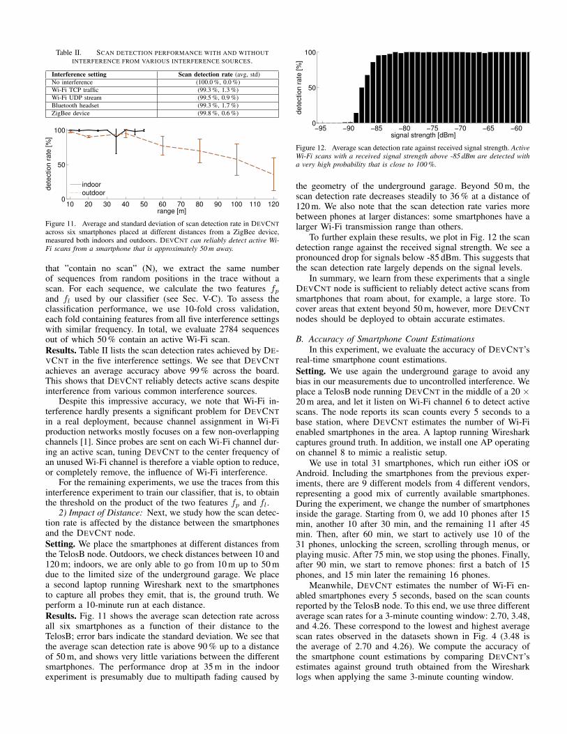
Table II. SCAN DETECTION PERFORMANCE WITH AND WITHOUTINTERFERENCE FROM VARIOUS INTERFERENCE SOURCES.

Interference setting Scan detection rate (avg, std)No interference (100.0 %, 0.0 %)Wi-Fi TCP traffic (99.3 %, 1.3 %)Wi-Fi UDP stream (99.5 %, 0.9 %)Bluetooth headset (99.3 %, 1.7 %)ZigBee device (99.8 %, 0.6 %)

10 20 30 40 50 60 70 80 90 100 110 1200

50

100

range [m]

dete

ction r

ate

[%

]

indoor

outdoor

Figure 11. Average and standard deviation of scan detection rate in DEVCNTacross six smartphones placed at different distances from a ZigBee device,measured both indoors and outdoors. DEVCNT can reliably detect active Wi-Fi scans from a smartphone that is approximately 50 m away.

that ”contain no scan” (N), we extract the same numberof sequences from random positions in the trace without ascan. For each sequence, we calculate the two features fpand fl used by our classifier (see Sec. V-C). To assess theclassification performance, we use 10-fold cross validation,each fold containing features from all five interference settingswith similar frequency. In total, we evaluate 2784 sequencesout of which 50 % contain an active Wi-Fi scan.Results. Table II lists the scan detection rates achieved by DE-VCNT in the five interference settings. We see that DEVCNTachieves an average accuracy above 99 % across the board.This shows that DEVCNT reliably detects active scans despiteinterference from various common interference sources.

Despite this impressive accuracy, we note that Wi-Fi in-terference hardly presents a significant problem for DEVCNTin a real deployment, because channel assignment in Wi-Fiproduction networks mostly focuses on a few non-overlappingchannels [1]. Since probes are sent on each Wi-Fi channel dur-ing an active scan, tuning DEVCNT to the center frequency ofan unused Wi-Fi channel is therefore a viable option to reduce,or completely remove, the influence of Wi-Fi interference.

For the remaining experiments, we use the traces from thisinterference experiment to train our classifier, that is, to obtainthe threshold on the product of the two features fp and fl.

2) Impact of Distance: Next, we study how the scan detec-tion rate is affected by the distance between the smartphonesand the DEVCNT node.Setting. We place the smartphones at different distances fromthe TelosB node. Outdoors, we check distances between 10 and120 m; indoors, we are only able to go from 10 m up to 50 mdue to the limited size of the underground garage. We placea second laptop running Wireshark next to the smartphonesto capture all probes they emit, that is, the ground truth. Weperform a 10-minute run at each distance.Results. Fig. 11 shows the average scan detection rate acrossall six smartphones as a function of their distance to theTelosB; error bars indicate the standard deviation. We see thatthe average scan detection rate is above 90 % up to a distanceof 50 m, and shows very little variations between the differentsmartphones. The performance drop at 35 m in the indoorexperiment is presumably due to multipath fading caused by

−95 −90 −85 −80 −75 −70 −65 −600

50

100

signal strength [dBm]

de

tectio

n r

ate

[%

]

Figure 12. Average scan detection rate against received signal strength. ActiveWi-Fi scans with a received signal strength above -85 dBm are detected witha very high probability that is close to 100 %.

the geometry of the underground garage. Beyond 50 m, thescan detection rate decreases steadily to 36 % at a distance of120 m. We also note that the scan detection rate varies morebetween phones at larger distances: some smartphones have alarger Wi-Fi transmission range than others.

To further explain these results, we plot in Fig. 12 the scandetection range against the received signal strength. We see apronounced drop for signals below -85 dBm. This suggests thatthe scan detection rate largely depends on the signal levels.

In summary, we learn from these experiments that a singleDEVCNT node is sufficient to reliably detect active scans fromsmartphones that roam about, for example, a large store. Tocover areas that extent beyond 50 m, however, more DEVCNTnodes should be deployed to obtain accurate estimates.

B. Accuracy of Smartphone Count EstimationsIn this experiment, we evaluate the accuracy of DEVCNT’s

real-time smartphone count estimations.Setting. We use again the underground garage to avoid anybias in our measurements due to uncontrolled interference. Weplace a TelosB node running DEVCNT in the middle of a 20 ×20 m area, and let it listen on Wi-Fi channel 6 to detect activescans. The node reports its scan counts every 5 seconds to abase station, where DEVCNT estimates the number of Wi-Fienabled smartphones in the area. A laptop running Wiresharkcaptures ground truth. In addition, we install one AP operatingon channel 8 to mimic a realistic setup.

We use in total 31 smartphones, which run either iOS orAndroid. Including the smartphones from the previous exper-iments, there are 9 different models from 4 different vendors,representing a good mix of currently available smartphones.During the experiment, we change the number of smartphonesinside the garage. Starting from 0, we add 10 phones after 15min, another 10 after 30 min, and the remaining 11 after 45min. Then, after 60 min, we start to actively use 10 of the31 phones, unlocking the screen, scrolling through menus, orplaying music. After 75 min, we stop using the phones. Finally,after 90 min, we start to remove phones: first a batch of 15phones, and 15 min later the remaining 16 phones.

Meanwhile, DEVCNT estimates the number of Wi-Fi en-abled smartphones every 5 seconds, based on the scan countsreported by the TelosB node. To this end, we use three differentaverage scan rates for a 3-minute counting window: 2.70, 3.48,and 4.26. These correspond to the lowest and highest averagescan rates observed in the datasets shown in Fig. 4 (3.48 isthe average of 2.70 and 4.26). We compute the accuracy ofthe smartphone count estimations by comparing DEVCNT’sestimates against ground truth obtained from the Wiresharklogs when applying the same 3-minute counting window.

15 30 45 60 75 90 105

0

5

10

15

20

25

30

time [min]

num

ber

of devic

es

interaction

10 phones 20 phones 31 phones 31 phones 31 phones 16 phones 0 phones

ground truth

upper/lower estimate

avg. estimate

Figure 13. Estimated and real number of Wi-Fi enabled devices as smart-phones are being added and removed over time. DEVCNT provides accuratesmartphone count estimates, achieving an average accuracy of up to 91 %.

Results. Fig. 13 plots DEVCNT’s estimates and ground truthover time. We first note that the number of smartphones thatare physically present inside the garage is roughly doublethe number of smartphones in the ground truth. We attributethis to the fact that several phones performed very few activescans in the experiment, with intervals much larger than the3-minute counting window we use. In fact, 9 smartphones didissue less than 3 active scans during the whole experiment,predominately such with an Android version of 2.3.7 or lower.We could not expect this behavior based on our analysis oflarge real-world datasets in Sec. IV, as there is no informationavailable on silent smartphones.

Nevertheless, we observe from Fig. 13 that DEVCNT’sestimates closely match ground truth as smartphones are beingadded and removed. When considering the average estimate,DEVCNT achieves an accuracy of 68.9 % throughout the entire2-h experiment, which corresponds to an average absoluteerror of 3.0 smartphones. As mentioned earlier, we expectDEVCNT’s estimates to be more accurate when the numberof smartphones is higher. Our results confirm this expectation:Considering the interval between 45 min and 75 min in whichall 31 smartphones are present, and by taking into account thedifferent activity patterns, DEVCNT achieves an average accu-racy of 87.3 % (1.8 average absolute error) while all phonesare in stand-by mode, and an average accuracy of 90.5 % (1.65average absolute error) while 10 of the smartphones are active.

As one would expect, DEVCNT is less accurate than aWi-Fi-based solution (such as [5]), simply because it has lessinformation at its disposal. In return, DEVCNT preserves bydesign the privacy of smartphone users, which is a strong assetwhen it comes to acceptance by law and the population [23],[24]. Nevertheless, an accuracy of 70–90 % is sufficient formany applications we target, and comparable to what has beenreported in the literature, for example, when counting smart-phones using audio tones [15] or when fingerprinting a Wi-Fidriver [10]. We thus conclude that DEVCNT provides accurateestimates on the number of Wi-Fi enabled smartphones if themobility and usage profile of smartphones is known, which isa reasonable assumption in many applications [5], [11], [24].

Finally, we also logged performance counters throughoutthis experiment to study the processing overhead on the TelosBnode. We find that the TelosB node was processing for only1.7 % of the time. This shows that our novel signal processingpipeline is amenable to an efficient implementation even onseverely resource-constrained embedded devices.

0

10

20

30

40

50

60

70

devic

e c

ount estim

ate

break lecture lunch

lecture hall front

lecture hall rear

entrance

11:00 AM 11:30 AM 12:00 PM 12:30 PMtime of day

Figure 14. Estimated number of smartphones in a real world trial.

C. Real-world Test RunIn a final real-world trial, we deploy DEVCNT in a lecture

hall to show the applicability of the system in an uncontrolledenvironment. Such an environment presents a significant chal-lenge for DEVCNT because of two reasons. First, in a largerroom with many people carrying smartphones there are manymore signals to process on the nodes and hence processingtime might be high and reach the limits of the system. Second,the system is exposed to interference originating from differentsurrounding devices that might emit patterns that have not beenconsidered in the training step of the classifier.Setting. We install a multi-hop wireless network consisting ofthree DEVCNT nodes, a relay node, and a sink. We place twonodes inside the lecture hall, in the front and in the rear area;we put the third node outside at one of the two main entrances.The lecture hall has a size of 20 by 25 m. We observe APs onchannels 1, 6, and 11. To minimize the interference from theAPs, we let all DEVCNT nodes listen on Wi-Fi channel 8.

We let the system run from 11 AM to 1 PM, so we observe amorning break, half a lecture, and a lunch break. At 11:30 AMwe count by hand 111 students inside the lecture hall. Whilewe also set up two laptops running Wireshark, we note that inthis real-world setting it is impossible to reliably determine theground truth. This is due to vastly different reception ranges ofWi-Fi and ZigBee radios: While a Wi-Fi receiver may be ableto hear a probe from a weak sender (e.g., located in anotherroom), probes from this sender on adjacent channels are oftentoo weak to be heard by a ZigBee node at the same distance.Results. Fig. 14 shows the estimated smartphone counts overtime for the 3 DEVCNT nodes. Although we lack ground truth,we see that DEVCNT’s estimates throughout the deploymentclosely match our expectations and visual on-site observations.For instance, during the initial break at about 11:05 AM thereis a drop in the estimated smartphone counts, because a fewstudents leave the lecture hall. The peaks at the beginning andat the end of the lecture are due to students using their phonesmore intensively, which leads to smartphones performing moreactive scans. Furthermore, as expected, DEVCNT’s estimatesremain fairly stable during the lecture, and afterward drop tonumbers close to zero as almost all students leave for lunch.Looking at the node at the entrance, we see that it generallysees fewer smartphones, yet the periods where students enteror leave the hall before and after the lecture are clearly visible.

We further note that both nodes inside the lecture hall seeabout the same number of smartphones. This is in accordancewith the findings in Sec. VII-A2: Since one DEVCNT node canreliably detect devices within a radius of 50 m, a single node

would have been sufficient to cover the entire lecture hall.These results show that DEVCNT can sustain signals from

hundreds of Wi-Fi transmitters, as evident from our Wiresharklogs, and delivers meaningful estimates in a real-world trialthat resembles, for example, a retail or indoor concert setting.

VIII. DISCUSSIONDEVCNT estimates in real-time the number of Wi-Fi en-

abled smartphones within a given area. By detecting active Wi-Fi scans from RSSI traces, DEVCNT obtains these counts ina fully-passive, non-invasive, and privacy-preserving manner.

Any system relying on externally observable properties forcounting misses those smartphones that do not disclose theseproperties, and DEVCNT is no exception. As such, like othersolutions from academia [20] and industry [5], DEVCNT canonly see phones that have Wi-Fi enabled and may count Wi-Fitransmitters other than phones. However, in the environmentswe target including open streets, shops, and train stations, thefraction of laptops and tablets is typically rather smaller.

DEVCNT supports deployments across large areas throughmulti-hop communications. In those scenarios, multiple Zig-Bee devices may detect and then count the same smartphone.A practical approach to ameliorate this over-counting problemwould be to carefully select the locations of the ZigBee devicesso as to reduce areas of overlapping reception ranges. Anotherpossibility would be to exploit the fact that DEVCNT devicesare time-synchronized, so an active scan that is detected bydifferent devices at the same time likely originates from thesame smartphone and could be accounted for only once. Weintend to explore this idea in our future work.

DEVCNT preserves the privacy of smartphone users as itcannot identify individual phones. While this is arguably a de-sirable property, it leaves DEVCNT with no other option than toestimate the smartphone counts based on statistical informationabout the average active scan rate. DEVCNT provides accurateestimates whenever the observed population of smartphonesbehaves according to the expectations, for example, in termsof their degree of mobility and how frequently the smartphonesare being used. If phones behave sharply differently, however,DEVCNT’s estimates may become less accurate. Nevertheless,we found in our tests that phases of unusual behavior typicallylast for only a limited amount of time as visible, for example, inFig. 14 right after the break. In that sense, DEVCNT is similarto participatory sensing approaches [27], where the availableGPS data fluctuate because smartphone users have full controlover the application and are free to opt out at any time.

The flexibility of battery-powered nodes is not for free: Tocapture as many active scans as possible, all DEVCNT nodesneed to have their radio continuously turned on. In this case,a node powered by two AA batteries would last for a week,which is fine for short deployments (e.g., during a concert).One way to save energy would be to turn off the radio forextended periods of time when there is low Wi-Fi activity,such as during the night or outside of a shop’s opening hours.We leave such energy considerations for future work.

Overall, DEVCNT represents a new point in a multi-dimen-sional design space, trading some fidelity of the smartphonecounts for full privacy of the smartphone users. Correspondingto this promising design point is a large number of applica-tion scenarios, ranging from crowd management [11] throughpublic transport and event planning [4] to customer and visitorsurveys [5], where DEVCNT could be highly beneficial.

IX. RELATED WORKOur work on DEVCNT is related to prior efforts on

leveraging the proliferation of smartphones for crowd countingand exploiting the interference between Wi-Fi and ZigBee.Leveraging smartphones for crowd counting. Existing solu-tions employ different observable properties of a smartphone tocount the number of people in an area or estimate the densityof crowds. Such properties include audio tones [15], GPScoordinates [27], Bluetooth scans [26], and Wi-Fi probes [5],[20]. Conceptually, we can classify these solutions along threedimensions: privacy, invasiveness, and passiveness.

Both research [20] and commercial [5] systems exist thatdirectly eavesdrop on Wi-Fi probes, using existing APs and/ordedicated Wi-Fi monitors. Being able to demodulate and de-code Wi-Fi frames, these systems can easily identify and trackindividual smartphones based on the unique MAC addressesembedded in each probe. Although anonymization techniquessuch as MAC address hashing are apparently used [5], thesesystems may still be exploited (e.g., by an attacker) to com-promise the privacy of the smartphone users, who possess nomeans to “see” that they are being observed. Turning off Wi-Fiis therefore the only practical solution to guard against suchimpairment, but this may impact user experience [3].

Another class of approaches requires to modify the smart-phone itself, for example, by installing and running a dedicatedapplication. The system presented in [15] uses the built-inmicrophones to count smartphones by letting them exchangebit patterns encoded in audio tones. Others estimate crowddensities based on GPS data [27] or the number of discovereddevices by Bluetooth scans [26]. These approaches are invasiveand rely on the voluntary and enduring cooperation of usersto produce meaningful estimates. Finally, [20] shows that it ispossible to solicit more probe transmissions from unmodifiedsmartphones to improve tracking performance.

Unlike these prior works, DEVCNT takes a fully-passive,non-invasive, and privacy-preserving counting approach. Thisapproach relies on DEVCNT taking advantage of interferencebetween ZigBee and Wi-Fi, similar to other systems that arehowever designed for different purposes, as discussed next.Exploiting interference between ZigBee and Wi-Fi. SoNICclassifies interference in the 2.4 GHz band into ”Wi-Fi,” ”mi-crowave,” or ”Bluetooth” based on RSSI information availableon a ZigBee device [12]. SpeckSense and ZiFi exploit inter-ference from Wi-Fi beacon frames, which are easier to detectthan active scans because they exhibit a more rigid periodicity.SpeckSense processes RSSI information on a TelosB device inorder to avoid Wi-Fi interference [14]. ZiFi uses a built-in orexternal ZigBee radio to help a smartphone or laptop discoverWi-Fi APs in a more energy-efficient manner [29]. Differentfrom DEVCNT, ZiFi benefits from ample resources of the hostdevice compared to the limited memory and compute powerof a low-power ZigBee mote. WizNet uses interference fromprobes, beacons, and other Wi-Fi traffic to monitor the spatio-temporal performance variations of Wi-Fi installations [28].Similar to DEVCNT, WizNet uses, among other techniques, thediscrete autocorrelation to identify probes from RSSI samples.However, unlike DEVCNT, WizNet sends compressed RSSItraces to a more capable sink for computing the autocorrelationoffline. DEVCNT shows that active scan detection can indeedbe performed online on mote-class devices, thereby reducingcommunication energy costs and bandwidth requirements bysending only the minimum amount of data to the sink.

X. CONCLUSIONSWe have presented DEVCNT, the first system that supports

real-time counting of unmodified Wi-Fi enabled smartphoneswhile preserving the privacy of the smartphone owners. Usingnovel signal processing algorithms that execute on a multi-hopnetwork of ZigBee devices, DEVCNT detects and counts activeWi-Fi scans performed by smartphones based on characteristicpatterns in RSSI traces. Combining these counts with statisticalinformation about the average active scanning rate, DEVCNTfaithfully estimates the number of Wi-Fi enabled smartphones.DEVCNT trades some fidelity in the smartphone count estima-tions for improved privacy. Results from controlled and real-world experiments show that DEVCNT provides estimates withan accuracy of up to 91 %. We thus maintain that DEVCNT isa viable and promising solution for low-cost, real-time crowdcounting in a broad spectrum of innovative applications.

ACKNOWLEDGEMENTSWe thank Marco V. Barbera for providing us with helpful

information about the datasets used in Sec. IV. The work pre-sented in this paper was scientifically evaluated by the SNSF,and financed by the Swiss Confederation and by nano-tera.ch.

REFERENCES

[1] A. Akella, G. Judd, S. Seshan, and P. Steenkiste. Self-management inchaotic wireless deployments. In Proc. of the 11th Intl. Conf. on MobileComputing and Networking (MobiCom), 2005.

[2] M. V. Barbera, A. Epasto, A. Mei, S. Kosta, V. C. Perta, and J. Stefa.CRAWDAD data set sapienza/probe-requests (v. 2013-09-10). Down-loaded from http://crawdad.org/sapienza/probe-requests/, Sept. 2013.

[3] M. V. Barbera, A. Epasto, A. Mei, V. C. Perta, and J. Stefa. Signalsfrom the crowd: Uncovering social relationships through smartphoneprobes. In Proc. of the Internet Measurement Conf. (IMC), 2013.

[4] C. C. Cheong and R. To. Household interview surveys from 1997 to2008—a decade of changing travel behaviours, May 2010. Online athttp://goo.gl/aw3WFV.

[5] Cisco Systems. White paper: CMX Analytics, Apr. 2014.[6] R. O. Duda, P. E. Hart, and D. G. Stork. Pattern Classification (2nd

Edition). Wiley-Interscience, 2001.[7] A. Dunkels, B. Gronvall, and T. Voigt. Contiki - a lightweight and

flexible operating system for tiny networked sensors. In Proc. of the1st IEEE Workshop on Embedded Networked Sensors (Emnets), 2004.

[8] Ericsson AB. Ericsson mobility report, June 2014.[9] F. Ferrari, M. Zimmerling, L. Thiele, and O. Saukh. Efficient network

flooding and time synchronization with Glossy. In Proc. of the 10thIntl. Conf. on Information Processing in Sensor Networks (IPSN), 2011.

[10] J. Franklin, D. McCoy, P. Tabriz, V. Neagoe, J. Van Randwyk, andD. Sicker. Passive data link layer 802.11 wireless device driverfingerprinting. In Proc. of the 15th USENIX Security Symposium (SS),2006.

[11] D. Helbing, L. Buzna, A. Johansson, and T. Werner. Self-organizedpedestrian crowd dynamics: Experiments, simulations, and design so-lutions. Transportation Science, 39(1):1–24, 2005.

[12] F. Hermans, O. Rensfelt, T. Voigt, E. Ngai, L.-A. Norden, and P. Gun-ningberg. SoNIC: Classifying interference in 802.15.4 sensor networks.In Proc. of the 12th Intl. Conf. on Information Processing in SensorNetworks (IPSN), 2013.

[13] W. Hu, T. Tan, L. Wang, and S. Maybank. A survey on visualsurveillance of object motion and behaviors. IEEE Trans. Syst., Man,Cybern. C, 34(3):334–352, 2004.

[14] V. Iyer, F. Hermans, and T. Voigt. Detecting and avoiding multiplesources of interference in the 2.4 GHz spectrum. In Proc. of the 12thIntl. Conf. on Embedded Wireless Systems and Networks (EWSN), 2015.

[15] P. G. Kannan, S. P. Venkatagiri, and M. C. Chan. Low cost crowdcounting using audio tones. In Proc. of the 10th ACM Conf. onEmbedded Networked Sensor Systems (SenSys), 2012.

[16] O. Landsiedel, F. Ferrari, and M. Zimmerling. Chaos: Versatile andefficient all-to-all data sharing and in-network processing at scale. InProc. of the 11th ACM Conf. on Embedded Networked Sensor Systems(SenSys), 2013.

[17] C.-J. M. Liang, N. B. Priyantha, J. Liu, and A. Terzis. Surviving Wi-Fiinterference in low power ZigBee networks. In Proc. of the 8th ACMConf. on Embedded Networked Sensor Systems (SenSys), 2010.

[18] R. Lim, F. Ferrari, M. Zimmerling, C. Walser, P. Sommer, and J. Beutel.FlockLab: A testbed for distributed, synchronized tracing and profilingof wireless embedded systems. In Proc. of the 12th Intl. Conf. onInformation Processing in Sensor Networks (IPSN), 2013.

[19] C. C. D. Loh, C. Y. Cho, C. P. Tan, and R. S. Lee. Identifying uniquedevices through wireless fingerprinting. In Proc. of the 1st ACM Conf.on Wireless Network Security (WiSec), 2000.

[20] A. B. M. Musa and J. Eriksson. Tracking unmodified smartphonesusing Wi-Fi monitors. In Proc. of the 10th ACM Conf. on EmbeddedNetworked Sensor Systems (SenSys), 2012.

[21] J. Polastre, R. Szewczyk, and D. Culler. Telos: Enabling ultra-lowpower wireless research. In Proc. of the 4th Intl. Conf. on InformationProcessing in Sensor Networks (IPSN), 2005.

[22] Texas Instruments. CC2420 datasheet, 2014.[23] The Guardian. City of London Corporation wants ’spy bins’ ditched,

Aug. 2013. Online at http://www.theguardian.com/world/2013/aug/12/city-london-corporation-spy-bins.

[24] The Local Denmark. Copenhagen to roll out new smart traf-fic system, Feb. 2015. Online at http://www.thelocal.dk/20150202/copenhagen-to-roll-out-new-smart-traffic-systems.

[25] The New York Times. Stampede at german music festival kills 18,July 2010. Online at http://www.nytimes.com/2010/07/25/world/europe/25germany.html.

[26] J. Weppner, P. Lukowicz, U. Blanke, and G. Troster. ParticipatoryBluetooth scans serving as urban crowd probes. IEEE Sensors Journal,14(12):4196–4206, 2014.

[27] M. Wirz, T. Franke, E. Mitleton-Kelly, D. Roggen, P. Lukowicz, andG. Troster. CoenoSense: A framework for real-time detection andvisualization of collective behaviors in human crowds by trackingmobile devices. In Proc. of the European Conf. on Complex Systems(ECCS), 2012.

[28] R. Zhou, G. Xing, X. Xu, J. Wang, and L. Gu. WizNet: A ZigBee-basedsensor system for distributed wireless LAN performance monitoring.In Intl. Conf. on Pervasive Computing and Communications (PerCom),2013.

[29] R. Zhou, Y. Xiong, G. Xing, L. Sun, and J. Ma. ZiFi: Wireless LANdiscovery via ZigBee interference signatures. In Proc. of the 16th Intl.Conf. on Mobile Computing and Networking (MobiCom), 2010.

APPENDIXWe further detail the algorithm used in DEVCNT to effi-

ciently compute the sum of autocorrelations feature fp.We know from Sec. V-C that this feature is defined as

fp =

w−a∑j=1

min(w,j+b)∑k=j+a

xjxk. (3 revisited)

Here, the xi are elements of a binary vector X ∈ {0, 1}w,indicating for each sample in the detection window of size wwhether there is a signal present or not. The symbols a and bdenote the limits for the lags of the autocorrelation function. Inaddition, we define l as the increasingly ordered set of indexesof value changes in the binary vector X , that is, l := {i|xi 6=xi+1}. In the following, we use the notation ls to refer to theelement in l at position s. Note that l changes from 0 to 1 atodd positions, while it changes from 1 to 0 at even positions.

A. Illustrative ExampleWe motivate our algorithm with the help of the example

illustrated in Fig. 15. Here, X contains four signals, whichresults in a set l of size 8, as shown on the vertical and thehorizontal axes. The elements to be summed up, xjxk, are laidout in a 2-dimensional bitmap. Dark boxes indicate elementsthat contribute to the sum, that is, where both xk and xj are1. The limits of the covered area are determined by [a, b], theinterval of the considered lags of the autocorrelation.

1 1 1 1 1 1 1 1 1 1 1 1 10 0 0 0 0 0 0 0 0 0 0 0 0 0 0 0 0 0 0k

j

111

111

1111

111

0000

00

0000000

00

0000

xb+1 x

w

x1

xw-a

xa+1

X

l1

l2

l3

l4

l5

l6

l7

l8

l1

l2

l3

l4

l5

l6

l7

l8

{o

A

B

Figure 15. Sum of autocorrelations for an example binary vector X . Theboxes represent all the xjxk that are added up in (3). Black boxes are theelements that contribute to the sum. The area of adjacent black boxes can becalculated without iterating over every element therein.

To compute the feature fp, we add up the areas of (partial)black rectangles formed by one or more adjacent black boxes.The area of the completely black rectangle A is the productof its length and width, that is, Area( A ) = (l6− l5)(l4− l3).The area of partially black rectangles, such as B , can also becalculated without iterating over every element by consideringthe offset o of the diagonal through the rectangle.

For our purpose, converting X into the set of value changeindexes l reduces both space requirements and computationalcomplexity: A detection window of 580 ms sampled with aresolution of 16µs results in a binary vector X of 36250 bits(8.53 kB). According to our experiments, the number of signalsin a detection window is rather small, and therefore the set lis significantly smaller than |X|. The reduced input size alsoreduces the complexity of the algorithm as we do not need toiterate over all samples in X , but only over the elements in l.

B. Algorithm and PseudocodeAlgorithm 1 calculates fp. It iterates over both dimensions

j and k using l, and sums up the rectangles delimited bythe corners (lk, lj)(lk+1, lj+1). An odd position in l indicates

the start of a signal, and an even position indicates the endof a signal. Thus, for every iteration, the index variables jand k are incremented by 2 to select the next rectangle. Wedistinguish three cases: (i) a fully contained rectangle (line 7),(ii) a rectangle partially outside on the lower end of k (line11), and (iii) a rectangle partially outside the upper end ofk (line 15). For (i) the number of elements is the productof the width and the height. For (ii) and (iii), the functionPartialRectangle() shown in Algorithm 2 additionally usesthe offset o to calculate the number of elements that fall intothis partial rectangle. In each iteration, the contribution of thecurrent rectangle is added to the final result fp.

Algorithm 1 Compute the Sum of Autocorrelations FeatureInput: l: indexes of level changes, a b: limits for lagOutput: fp: sum of autocorrelation between a and b

1: fp ← 02: j ← 13: while j < |l| do4: k ← 15: while k < |l| do6: if lk ≥ lj+1 + a− 1 and lk+1 ≤ lj + b+ 1 then7: fp ← fp + (lk+1 − lk)(lj+1 − lj)8: else9: if lk < lj+1 + a− 1 and lk+1 > lj + a then

10: o← lk − lj − a+ 111: fp ← fp +PartialRectangle(lk+1 − lk, lj+1 − lj , o)12: else13: if lk > lj+1 + b and lk+1 > lj + b+ 1 then14: o← lj+1 − lk+1 + b+ 115: fp ← fp+PartialRectangle(lk+1−lk, lj+1−lj , o)16: end if17: end if18: end if19: k ← k + 220: end while21: j ← j + 222: end while

Algorithm 2 PartialRectangle(o, w1, w2)Input: w1, w2: width and height of area, o: offset of diagonalOutput: A: number of elements contained in area

1: if o > 0 then2: A0 ← w1o3: d1 ← w1 − 14: else5: A0 ← 06: d1 ← w1 + o− 17: end if8: d2 ← max(1, w1 − (w2 − o))9: A← A0 + (d1 + d2)(d1 − d2 + 1)/2