Parts Assembly Planning under Uncertainty

with Simulation-Aided Physical Reasoning

Sung-Kyun Kim, Maxim Likhachev

The Robotics Institute

Carnegie Mellon University

{kimsk,maxim}@cs.cmu.edu

Abstract— Parts assembly, in a broad sense, is to makemultiple objects to be in specific relative poses in contactwith each other. One of the major reasons that make itdifficult is uncertainty. Because parts assembly involves physicalcontact between objects, it requires higher precision than othermanipulation tasks like collision avoidance. The key idea ofthis paper is to use simulation-aided physical reasoning whileplanning with the goal of finding a robust motion plan forparts assembly. Specifically, in the proposed approach, a)uncertainty between object poses is represented as a distributionof particles, b) the motion planner estimates the transition ofparticles for unit actions (motion primitives) through physics-based simulation, and c) the performance of the planner issped up using Multi-Heuristic A* (MHA*) search that utilizesmultiple inadmissible heuristics that lead to fast uncertaintyreduction. To demonstrate the benefits of our framework,motion planning and physical robot experiments for severalparts assembly tasks are provided.

I. INTRODUCTION

Parts assembly is happening not only in factories but alsoin most of our living spaces. It is an operation of arranging,stacking, or combining objects. Many physical manipulationtasks that are to set relative poses between multiple objectsin contact can be considered as parts assembly in a broadsense.

The challenge, however, is that contact involves complexphysical phenomena such as friction and force interaction inaddition to kinematics and dynamics of objects. These phe-nomena are hard to estimate or approximate well. Moreover,parts assembly usually requires higher precision in motionbecause it is a practice of placing objects to fit in, notseparating them apart.

Therefore, it is important to reason about the underlyingphysics and to execute manipulation plans that are robustto uncertainty during assembly. In this paper, we propose aframework to utilize a physics-based simulator for physicalreasoning and use graph search algorithms to find a robustmotion plan in belief space.

The rationale behind selecting a simulator for physicalreasoning is that modeling complex manipulation actionsto sufficient degree of fidelity is infeasible. Instead, weshould exploit state-of-the-art in physics-based simulationwhile planning.

This research was sponsored by ARL, under the Robotics CTA programgrant W911NF-10-2-0016.

By sampling uncertainty distribution and running physics-based simulation of actions, the planner constructs a beliefspace. The planner then runs a heuristic search to find aplan while reducing the uncertainty for a higher chance ofsuccess.

This paper is organized as follows: Section II reviewsthe related work in parts assembly and planning underuncertainty. Section III explains some background aboutgraph search and describes how a simulator is integrated witha motion planner for physical reasoning. Section IV providesthe detailed formulation and algorithm of the motion plan-ning, and section V shows experimental results for severalparts assembly tasks. Section VI concludes the paper.

II. RELATED WORK

Since parts assembly is an essential manipulation task,research about parts assembly has a long history. Someearlier works were about part feeding that utilized contactbetween an object and the environment to adjust its pose [1],[2]. Basically, these approaches tried to reduce uncertaintyin object orientation on a plane by a sequence of actions.They required rigorous analysis of configuration space thatparticularly depended on the shape of the object and wasonly possible in 2D space.

More recent works inheriting this scheme can be found in[3] and [4]. In these works, the robot exploits contact withthe environment or other objects for robust grasping or in-hand manipulation. (It is called extrinsic dexterity in [3].) Asin this paper, they rely on the idea of using contact to reduceuncertainty and successfully demonstrate its effectiveness.However, the motions being used are hand-scripted and thereis no general motion planner.

In [5], [6], works on parts assembly by multiple robots arepresented. They propose an architecture for parts assemblyand failure recovery. It is a high-level symbolic planner, so ittreats the actual manipulation as a simple operation and doesnot account for physical phenomena during parts assembly.

On the other hand, there is an abundance of work onplanning under uncertainty, An example is collision avoid-ance under uncertainty [7]. The other example is uncertaintyreduction in localization by getting closer to landmarks orbeacons [8], [9]. Both can also be pursued simultaneously[10], [11], [12]. In either case, they don’t presume any

Physics-based Simulator

...

(pr, Rr)(p01, R01)

(p0n, R0n)

...

particle1

(pr, Rr)(p01, R01)

(p0n, R0n)

...

(pr, Rr)(p01, R01)

(p0n, R0n)

...

belief i

...

(pr, Rr)(p01, R01)

(p0n, R0n)

...

(pr, Rr)(p01, R01)

(p0n, R0n)

...

(pr, Rr)(p01, R01)

(p0n, R0n)

...

belief i+k

k-th motionprimitive

k-th motionprimitive

k-th motionprimitive

particle2 particlem

particle1 particle2 particlem

1st motionprimitive

. . . ...

2nd motionprimitive

K-th motionprimitive

(K-1)-th motionprimitive

belief i+1

belief i+2

belief i+K

belief i+K-1

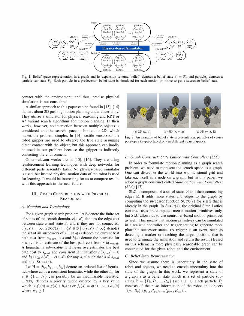
Fig. 1: Belief space representation in a graph and its expansion scheme. belief i denotes a belief state si = Pi, and particlej denotes a

particle sub-state Pj . Each particle in a predecessor belief state is simulated for each motion primitive to get a successor belief state.

contact with the environment, and thus, precise physicalsimulation is not considered.

A similar approach to this paper can be found in [13], [14]that are about 2D pushing motion planning under uncertainty.They utilize a simulator for physical reasoning and RRT orA* variant search algorithms for motion planning. In theirworks, however, no interaction between multiple objects isconsidered and the search space is limited to 2D, whichmakes the problem simpler. In [14], tactile sensors of therobot gripper are used to observe the true state assumingdirect contact with the object, but this approach can hardlybe used in our problem because the gripper is indirectlycontacting the environment.

Other relevant works are in [15], [16]. They are usingreinforcement learning techniques with deep networks fordifferent parts assembly tasks. No physics-based simulatoris used, but instead physical motion data of the robot is usedfor learning. It would be interesting for us to compare resultswith this approach in the near future.

III. GRAPH CONSTRUCTION WITH PHYSICAL

REASONING

A. Notation and Terminology

For a given graph search problem, let S denote the finite setof states of the search domain. c(s, s′) denotes the edge costbetween state s and state s′, and if they are not connected,c(s, s′) = ∞. SUCC(s) := {s′ ∈ S | c(s, s′) = ∞} denotesthe set of all successors of s. Let g(s) denote the current bestpath cost from sstart to s and h(s) denote the heuristic fors which is an estimate of the best path cost from s to sgoal.A heuristic is admissible if it never overestimates the bestpath cost to sgoal and consistent if it satisfies h(sgoal) = 0and h(s) ≤ h(s′) + c(s, s′) for any s, s′ such that s = sgoaland s′ ∈ SUCC(s).

Let H = [h0, h1, ..., hN ] denote an ordered list of heuris-tics where h0 is a consistent heuristic, while the other hv forv ∈ {1, ..., N} can possibly be an inadmissible heuristic.OPENv denotes a priority queue ordered by a key valuewhich is fv(s) = g(s)+hv(s) or fv(s) = g(s)+w1 ∗hv(s)where w1 ≥ 1.

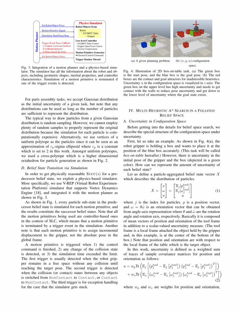
(a) 2D (x, y) (b) 3D (x, y, z) (c) 3D (y, z, R)

Fig. 2: An example of belief state representation: particles of cross-polytopes (hyperoctahedron) in different search spaces.

B. Graph Construct: State Lattice with Controllers (SLC)

In order to formulate motion planning as a graph searchproblem, we need to represent the search space as a graph.One can discretize the world into n-dimensional grid andtake each cell as a node on a graph, but in this paper, weadopt a graph construct called State Lattice with Controllers

(SLC) [17].SLC is composed of a set of states S and their connecting

edges E. It adds more states and edges to the graph bycomputing the successor function SUCC(s) for s ∈ S that isalready in the graph. In SUCC(s), the original State Latticeconstruct uses pre-computed metric motion primitives only,but SLC allows us to use controller-based motion primitivesas well. This means that motion primitives can be simulatedin a realistic controller and trigger setting to generate moreplausible successor states. (A trigger is an event, such asdetecting a marker or reaching the target position, that isused to terminate the simulation and return the result.) Basedon this scheme, a more physically reasonable graph can beconstructed for the given robot and the environment.

C. Belief State Representation

Since we assume there is uncertainty in the state ofrobot and objects, we need to encode uncertainty into thestate of the graph. In this work, we represent a state ofa graph s as a belief state which is a set of particle sub-states P = {P0, P1, ..., Pm} (see Fig. 1). Each particle Pj

consists of the pose information of the robot and objects{(pr, Rr), (po1, Ro1), ..., (pon, Ron)}.

Physics Simulator

Robot XYZRPY Table Gripper

Low-level Controller - XYZRPY Table Control - Gripper Open/Close Control - Gravity Compensation

Motion Primitive Signal

Set Robot/Object Poses

Simulation Start/Pause/Stop

Trigger Event Topic Callback 1) Control command finished 2) Collision detected 3) Time passed the limit Motion Primitive Generator

➔ Desired Control CommandGet Robot/Object PosesTrigger Monitor Thread

Mot

ion

Plan

ner

Robot-Objects Scene

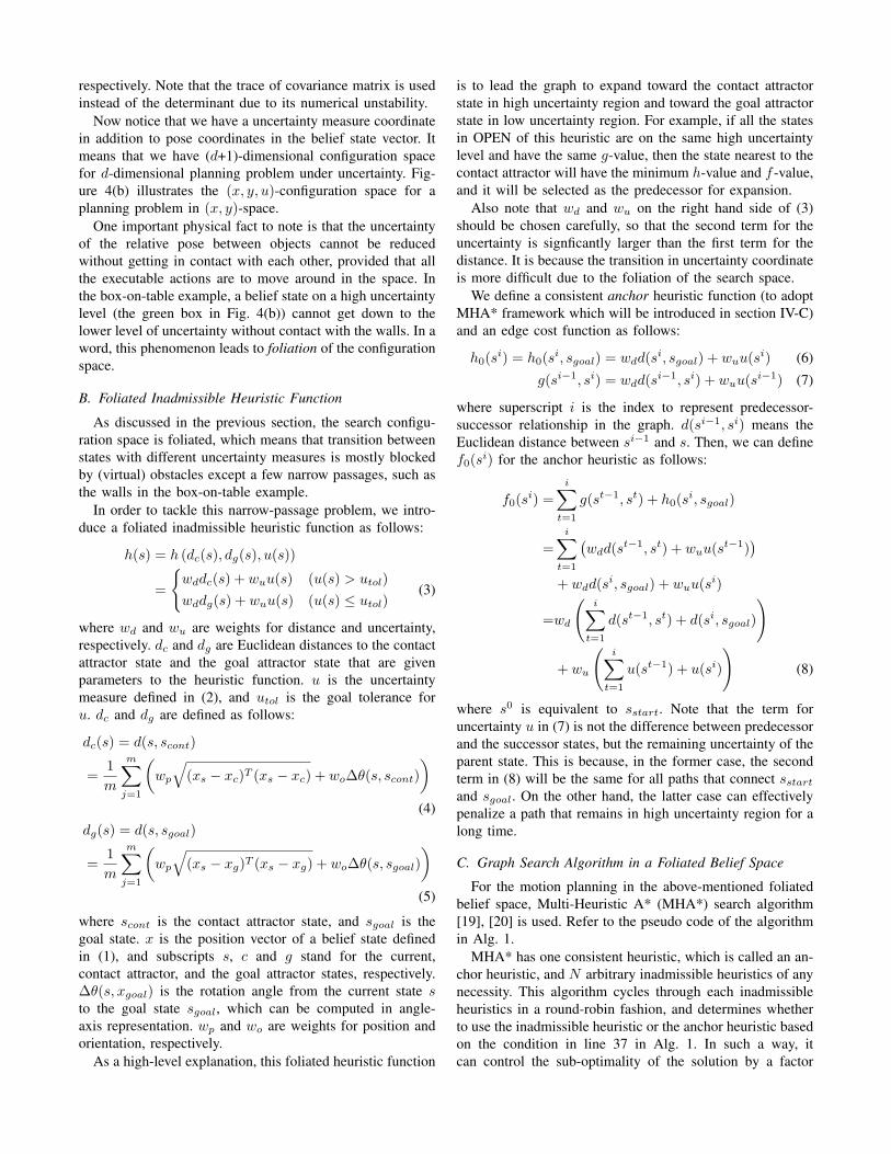
Fig. 3: Integration of a motion planner and a physics-based simu-lator. The simulator has all the information about the robot and ob-jects, including geometric shapes, inertial properties, and controllercharacteristics. Simulation of a motion primitive is terminated ifone of the trigger events is detected.

For parts assembly tasks, we accept Gaussian distributionas the initial uncertainty of a given task, but note that anydistributions can be used as long as the number of particlesare sufficient to represent the distribution.

The typical way to draw particles from a given Gaussiandistribution is random sampling. However, we cannot employplenty of random samples to properly represent the originaldistribution because the simulation for each particle is com-putationally expensive. Alternatively, we use vertices of auniform polytope as the particles since it can be seen as anapproximation of cp-sigma ellipsoid where cp is a constantwhich is set to 2 in this work. Amongst uniform polytopes,we used a cross-polytope which is a higher dimensionaloctahedron for particle generation as shown in Fig. 2.

D. Belief State Transition via Simulation

In order to get physically reasonable SUCC(s) for a pre-decessor belief state, we exploit a physics-based simulator.More specifically, we use V-REP (Virtual Robot Experimen-tation Platform) simulator that supports Vortex DynamicsEngine [18], and integrated it with the motion planner asshown in Fig. 3.

As shown in Fig. 1, every particle sub-state in the prede-cessor belief state is simulated for each motion primitive, andthe results constitute the successor belief states. Note that allthe motion primitives being used are controller-based onesin the context of SLC, which means that a motion primitiveis terminated by a trigger event in the simulation. Anothernote is that each motion primitive is to assign incrementaldisplacement to the gripper, not the absolute pose in theglobal frame.

A motion primitive is triggered when 1) the controlcommand is finished, 2) any change of the collision stateis detected, or 3) the simulation time exceeded the limit.The first trigger is usually detected when the robot grip-per remains in a free space without any collision untilreaching the target pose. The second trigger is detectedwhen the collision (or contact) states between any objectsis switched from NonContact to Contact, or Contactto NonContact. The third trigger is for exception handlingfor the case that the simulator gets stuck.

(a) A given planning problem. (b) (x, y, u)-configuration

space.

Fig. 4: Illustration of 2D box-on-table task. (a) The green boxis the start pose, and the blue box is the goal pose. (b) The redboxes are the contact and goal attractors for inadmissible heuristics.Uncertainty u in the configuration space is visualized in z-axis. Thegreen box on the upper level has high uncertainty and needs to getcontact with the walls to reduce pose uncertainty and get down tothe lower level of uncertainty where the goal state exists.

IV. MULTI-HEURISTIC A* SEARCH IN A FOLIATED

BELIEF SPACE

A. Uncertainty in Configuration Space

Before getting into the details for belief space search, wedescribe the special structure of the configuration space underuncertainty.

First, let us take an example. As shown in Fig. 4(a), therobot gripper is holding a box and wants to place it at theposition of the blue box accurately. (This task will be calledbox-on-table hereafter.) However, there is uncertainty in theinitial pose of the gripper and the box (depicted in a greencolor). How can we represent the amount of uncertainty ofeach belief state?

Let us define a particle-aggregated belief state vector Xwhich describes the distribution of particles.

X =

⎡

⎣

xωu

⎤

⎦ =

⎡

⎣

Ej [ptoolj ]Ej [ωtool

j ]u

⎤

⎦ (1)

where j is the index for particles. p is a position vector,and ω = θω is an orientation vector that can be obtainedfrom angle-axis representation where θ and ω are the rotationangle and rotation axis, respectively. Basically it is composedof mean vectors of position and orientation of the tool framein addition to a scalar-valued uncertainty measure. (The toolframe is a local frame attached the object held by the gripperand, in this example, is at the center of the bottom of thebox.) Note that position and orientation are with respect tothe local frame of the table which is the target object.

In this work, uncertainty is defined as a weighted sumof traces of sample covariance matrices for position andorientation as follows:

u = wpTr(

Ej

[

(

ptoolj − Ej

[

ptoolj

]) (

ptoolj − Ej

[

ptoolj

])T])

+ woTr(

Ej

[

(

ωtoolj − Ej

[

ωtoolj

]) (

ωtoolj − Ej

[

ωtoolj

])T])

(2)

where wp and wo are weights for position and orientation,

respectively. Note that the trace of covariance matrix is usedinstead of the determinant due to its numerical unstability.

Now notice that we have a uncertainty measure coordinatein addition to pose coordinates in the belief state vector. Itmeans that we have (d+1)-dimensional configuration spacefor d-dimensional planning problem under uncertainty. Fig-ure 4(b) illustrates the (x, y, u)-configuration space for aplanning problem in (x, y)-space.

One important physical fact to note is that the uncertaintyof the relative pose between objects cannot be reducedwithout getting in contact with each other, provided that allthe executable actions are to move around in the space. Inthe box-on-table example, a belief state on a high uncertaintylevel (the green box in Fig. 4(b)) cannot get down to thelower level of uncertainty without contact with the walls. In aword, this phenomenon leads to foliation of the configurationspace.

B. Foliated Inadmissible Heuristic Function

As discussed in the previous section, the search configu-ration space is foliated, which means that transition betweenstates with different uncertainty measures is mostly blockedby (virtual) obstacles except a few narrow passages, such asthe walls in the box-on-table example.

In order to tackle this narrow-passage problem, we intro-duce a foliated inadmissible heuristic function as follows:

h(s) = h (dc(s), dg(s), u(s))

=

{

wddc(s) + wuu(s) (u(s) > utol)

wddg(s) + wuu(s) (u(s) ≤ utol)(3)

where wd and wu are weights for distance and uncertainty,respectively. dc and dg are Euclidean distances to the contactattractor state and the goal attractor state that are givenparameters to the heuristic function. u is the uncertaintymeasure defined in (2), and utol is the goal tolerance foru. dc and dg are defined as follows:

dc(s) = d(s, scont)

=1

m

m∑

j=1

(

wp

√

(xs − xc)T (xs − xc) + wo∆θ(s, scont)

)

(4)

dg(s) = d(s, sgoal)

=1

m

m∑

j=1

(

wp

√

(xs − xg)T (xs − xg) + wo∆θ(s, sgoal)

)

(5)

where scont is the contact attractor state, and sgoal is thegoal state. x is the position vector of a belief state definedin (1), and subscripts s, c and g stand for the current,contact attractor, and the goal attractor states, respectively.∆θ(s, xgoal) is the rotation angle from the current state sto the goal state sgoal, which can be computed in angle-axis representation. wp and wo are weights for position andorientation, respectively.

As a high-level explanation, this foliated heuristic function

is to lead the graph to expand toward the contact attractorstate in high uncertainty region and toward the goal attractorstate in low uncertainty region. For example, if all the statesin OPEN of this heuristic are on the same high uncertaintylevel and have the same g-value, then the state nearest to thecontact attractor will have the minimum h-value and f -value,and it will be selected as the predecessor for expansion.

Also note that wd and wu on the right hand side of (3)should be chosen carefully, so that the second term for theuncertainty is signficantly larger than the first term for thedistance. It is because the transition in uncertainty coordinateis more difficult due to the foliation of the search space.

We define a consistent anchor heuristic function (to adoptMHA* framework which will be introduced in section IV-C)and an edge cost function as follows:

h0(si) = h0(s

i, sgoal) = wdd(si, sgoal) + wuu(s

i) (6)

g(si−1, si) = wdd(si−1, si) + wuu(s

i−1) (7)

where superscript i is the index to represent predecessor-successor relationship in the graph. d(si−1, si) means theEuclidean distance between si−1 and s. Then, we can definef0(si) for the anchor heuristic as follows:

f0(si) =

i∑

t=1

g(st−1, st) + h0(si, sgoal)

=i∑

t=1

(

wdd(st−1, st) + wuu(s

t−1))

+ wdd(si, sgoal) + wuu(s

i)

=wd

(

i∑

t=1

d(st−1, st) + d(si, sgoal)

)

+ wu

(

i∑

t=1

u(st−1) + u(si)

)

(8)

where s0 is equivalent to sstart. Note that the term foruncertainty u in (7) is not the difference between predecessorand the successor states, but the remaining uncertainty of theparent state. This is because, in the former case, the secondterm in (8) will be the same for all paths that connect sstartand sgoal. On the other hand, the latter case can effectivelypenalize a path that remains in high uncertainty region for along time.

C. Graph Search Algorithm in a Foliated Belief Space

For the motion planning in the above-mentioned foliatedbelief space, Multi-Heuristic A* (MHA*) search algorithm[19], [20] is used. Refer to the pseudo code of the algorithmin Alg. 1.

MHA* has one consistent heuristic, which is called an an-chor heuristic, and N arbitrary inadmissible heuristics of anynecessity. This algorithm cycles through each inadmissibleheuristics in a round-robin fashion, and determines whetherto use the inadmissible heuristic or the anchor heuristic basedon the condition in line 37 in Alg. 1. In such a way, itcan control the sub-optimality of the solution by a factor

S Gxh0

(a) A given problem: move balls at S to G.

Consistent anchor heuristic (h0).

S=S0 S1’

G=S6

S1 S2’S3

S4’S5

x

u

S4’

hα hβ

hg

h0 hβ hβhα� �� �

hg�

hg�S’PS

m m’Motion Primitives

(b) Inadmissible contact heuristics (hα and hβ ) and goal heuristic (hg).

Fig. 5: Illustration of a 1-dimensional toy example.

of w1 ∗ w2 where w1 and w2 are the weights for weightedA* search (in line 22) and anchor sub-optimality (in line 37).

To adopt MHA* for our problem, two major revisionsare made: particle generation/transition and attractor-basedheurisitics. As a belief space search problem, we need togenerate a set of particles and obtain reasonable transitionof them, which are explained in section III. For the foliatedbelief space, we need to find good (inadmissible) heuristicsthat can help the search to go through the narrow passagesfast, which can be in the form of (3) in section IV-B.

The heuristic function in (3) needs two input parameters,scont and sgoal, and they are being searched in ATTRAC-TORSEARCH(sseed) as shown in line 8 in Alg. 1. It is aquite simple operation that checks the amount of uncertaintyreduction after applying motion primitives. It can apply asingle long motion primitive or a sequence of them, and itcan start from sstart or sgoal. As of now it is a naive process,but can possibly be developed as a sophisticated one.

D. Toy Example

Let us take a look at a 1-dimensional toy example to seehow MHA* works in a foliated belief space. As shown inFig. 5(a), the initial belief state at S has high uncertaintyin x-position. From the belief state vector representation,we can construct a 2-dimensional configuration space withadditional u-coordinate as shown in Fig. 5(b). There are two

TABLE I: MHA* SEARCH PROCESS FOR A TOY EXAMPLE

Index Turn forRound-Robin

SatisfiedLine 37?

SelectorHeuristic

SelectedParent

ChildStates

1 α No h0 S0 = S S1, S1′

2 β Yes hβ S1′ S2′

3 α Yes hα S1 S3

4 β Yes hβ S2′ S4′

5 α Yes hg S4′ S5

6 β Yes hg S5 S6 = G

Algorithm 1 Multi-Heuristic A* Search in a Foliated BeliefSpace

Input: The start state sstart and the goal state sgoal, sub-optimalitybound factor w1, w2 (both ≥ 1), and one consistent heuristich0.

Output: A path from sstart to sgoal whose cost is within w1 ∗w2 ∗g∗(sgoal).

1: procedure CROSSPOLYTOPEPARTICLES(µ, Σ)2: create a nominal particle P0 from µ3: P← ∅4: for d ∈ SearchSpaceCoordinates do5: P← P ∪ {P0 + cp ∗ Σ(d,d)ed} ◃ {ed}: orthonormal

basis of SearchSpace6: P← P ∪ {P0 − cp ∗ Σ(d,d)ed}

7: return P

8: procedure ATTRACTORSEARCH(sseed)9: Sattractor ← ∅

10: for mk ∈ LongMotionPrimitives do11: s′ ← SUCC(sseed,mk)12: if s′.UNCERT() < cu ∗ sseed.UNCERT() then13: Sattractor ← Sattractor ∪ {s′}

14: return Sattractor

15: procedure NEWINADMISSHEURISTIC(sattractor , sgoal)16: create a new instance of a heuristic class, h′

17: h′.attractor← sattractor18: h′.goal← sgoal19: return h′

20: procedure KEY(s, v)21: hv ← H.GET(v)22: return g(s) + w1 ∗ hv(s)

23: procedure MAIN()24: sstart ← CROSSPOLYTOPEPARTICLES(µstart, Σstart)25: H← ∅, N ← 026: H.ADD(h0)27: for sattractor in ATTRACTORSEARCH(sstart) do28: H.ADD(NEWINADMISSHEURISTIC(sattractor , sgoal))29: N ← N + 130: g(sstart)← 0, g(sgoal)←∞31: for v = 0, 1, ..., N do32: OPENv ← ∅33: insert sstart in OPENv with KEY(sstart, v)

34: CLOSEDanchor ← ∅, CLOSEDinad ← ∅35: while OPEN0.MINKEY() <∞ do36: for v = 1, 2, ..., N do37: if OPENv .MINKEY() ≤ w2 * OPEN0.MINKEY()

then38: if g(sgoal) ≤ OPENv .MINKEY() then39: if g(sgoal) <∞ then40: terminate and return a solution path

41: else42: s← OPENv .TOP()43: EXPANDSTATE(s)44: insert s in CLOSEDinad

45: else46: if g(sgoal) ≤ OPEN0.MINKEY() then47: if g(sgoal) ≤ ∞ then48: terminate and return a solution path

49: else50: s← OPEN0.TOP()51: EXPANDSTATE(s)52: insert s in CLOSEDanchor

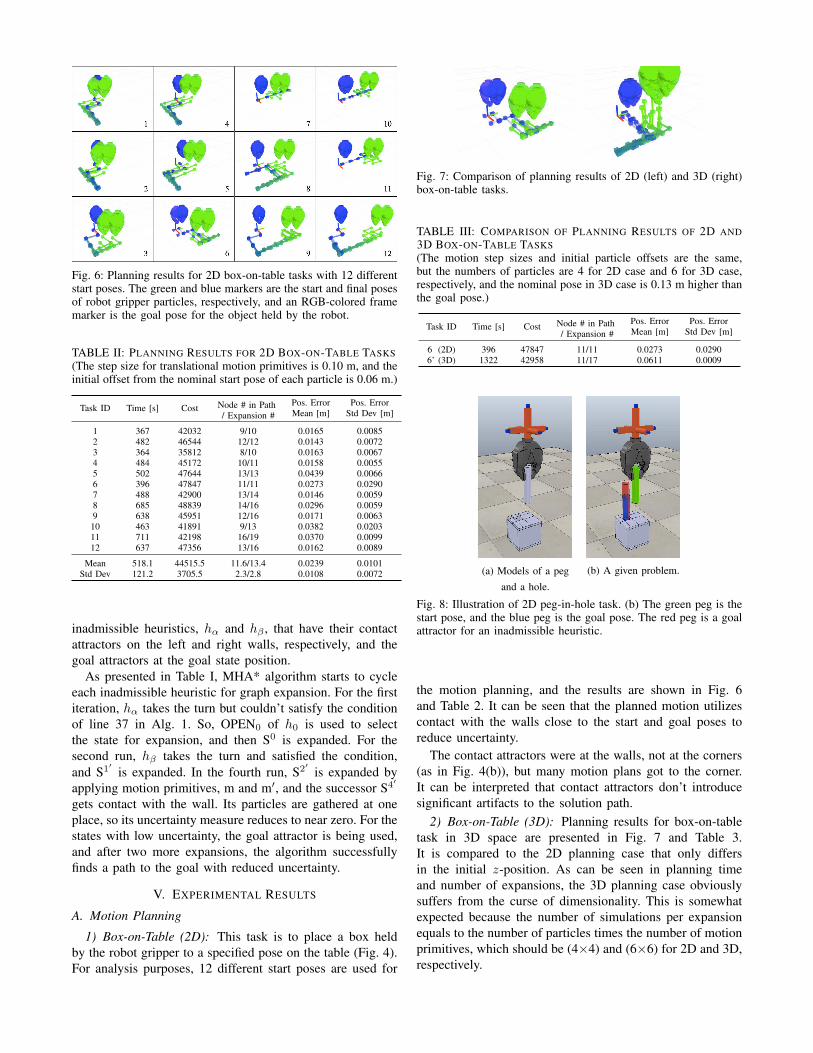
Fig. 6: Planning results for 2D box-on-table tasks with 12 differentstart poses. The green and blue markers are the start and final posesof robot gripper particles, respectively, and an RGB-colored framemarker is the goal pose for the object held by the robot.

TABLE II: PLANNING RESULTS FOR 2D BOX-ON-TABLE TASKS

(The step size for translational motion primitives is 0.10 m, and theinitial offset from the nominal start pose of each particle is 0.06 m.)

Task ID Time [s] Cost Node # in Path/ Expansion #

Pos. ErrorMean [m]

Pos. ErrorStd Dev [m]

1 367 42032 9/10 0.0165 0.00852 482 46544 12/12 0.0143 0.00723 364 35812 8/10 0.0163 0.00674 484 45172 10/11 0.0158 0.00555 502 47644 13/13 0.0439 0.00666 396 47847 11/11 0.0273 0.02907 488 42900 13/14 0.0146 0.00598 685 48839 14/16 0.0296 0.00599 638 45951 12/16 0.0171 0.006310 463 41891 9/13 0.0382 0.020311 711 42198 16/19 0.0370 0.009912 637 47356 13/16 0.0162 0.0089

Mean 518.1 44515.5 11.6/13.4 0.0239 0.0101Std Dev 121.2 3705.5 2.3/2.8 0.0108 0.0072

inadmissible heuristics, hα and hβ , that have their contactattractors on the left and right walls, respectively, and thegoal attractors at the goal state position.

As presented in Table I, MHA* algorithm starts to cycleeach inadmissible heuristic for graph expansion. For the firstiteration, hα takes the turn but couldn’t satisfy the conditionof line 37 in Alg. 1. So, OPEN0 of h0 is used to selectthe state for expansion, and then S0 is expanded. For thesecond run, hβ takes the turn and satisfied the condition,

and S1′

is expanded. In the fourth run, S2′

is expanded byapplying motion primitives, m and m′, and the successor S4

′

gets contact with the wall. Its particles are gathered at oneplace, so its uncertainty measure reduces to near zero. For thestates with low uncertainty, the goal attractor is being used,and after two more expansions, the algorithm successfullyfinds a path to the goal with reduced uncertainty.

V. EXPERIMENTAL RESULTS

A. Motion Planning

1) Box-on-Table (2D): This task is to place a box heldby the robot gripper to a specified pose on the table (Fig. 4).For analysis purposes, 12 different start poses are used for

Fig. 7: Comparison of planning results of 2D (left) and 3D (right)box-on-table tasks.

TABLE III: COMPARISON OF PLANNING RESULTS OF 2D AND

3D BOX-ON-TABLE TASKS

(The motion step sizes and initial particle offsets are the same,but the numbers of particles are 4 for 2D case and 6 for 3D case,respectively, and the nominal pose in 3D case is 0.13 m higher thanthe goal pose.)

Task ID Time [s] Cost Node # in Path/ Expansion #

Pos. ErrorMean [m]

Pos. ErrorStd Dev [m]

6 (2D) 396 47847 11/11 0.0273 0.02906’ (3D) 1322 42958 11/17 0.0611 0.0009

(a) Models of a peg

and a hole.

(b) A given problem.

Fig. 8: Illustration of 2D peg-in-hole task. (b) The green peg is thestart pose, and the blue peg is the goal pose. The red peg is a goalattractor for an inadmissible heuristic.

the motion planning, and the results are shown in Fig. 6and Table 2. It can be seen that the planned motion utilizescontact with the walls close to the start and goal poses toreduce uncertainty.

The contact attractors were at the walls, not at the corners(as in Fig. 4(b)), but many motion plans got to the corner.It can be interpreted that contact attractors don’t introducesignificant artifacts to the solution path.

2) Box-on-Table (3D): Planning results for box-on-tabletask in 3D space are presented in Fig. 7 and Table 3.It is compared to the 2D planning case that only differsin the initial z-position. As can be seen in planning timeand number of expansions, the 3D planning case obviouslysuffers from the curse of dimensionality. This is somewhatexpected because the number of simulations per expansionequals to the number of particles times the number of motionprimitives, which should be (4×4) and (6×6) for 2D and 3D,respectively.

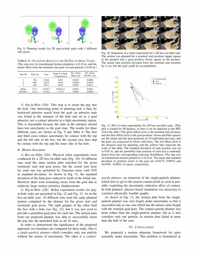
Fig. 9: Planning results for 2D peg-in-hole tasks with 3 differentstart poses.

TABLE IV: PLANNING RESULTS FOR 2D PEG-IN-HOLE TASKS

(The step size for translational motion primitives is 0.10 m, and theinitial offset from the nominal start pose of each particle is 0.04 m.)

Task ID Time [s] Cost Node # in Path/ Expansion #

Pos. ErrorMean [m]

Pos. ErrorStd Dev [m]

1 706 12164 16/21 0.0032 0.00092 604 12474 16/19 0.0029 0.00183 830 15311 22/25 0.0035 0.0011

Mean 713.1 13316.3 18.0/21.6 0.0032 0.0013Std Dev 113.2 1734.4 3.1/3.5 0.0003 0.0005

3) Peg-in-Hole (2D): This task is to insert the peg intothe hole. One interesting point of planning task is that, bybackward attractor search from the goal, an attractor statewas found at the entrance of the hole and set as a goalattractor, not a contact attractor in a high uncertainty region.This is reasonable because the state at the entrance shouldhave low uncertainty as the goal state. The results for threedifferent cases are shown in Fig. 9 and Table 4. The firstand third cases reduce uncertainty by contact with the topand the left side of the box, but the second case does thatby contact with the top and the inner side of the hole.

B. Motion Execution

1) Box-on-Table (2D): Physical robot experiments wereconducted for a 2D box-on-table task (Fig. 10). 10 differentruns used the same motion plan searched for the given(nominal) start and goal poses, but the actual start posefor each run was perturbed by Gaussian noise with 0.05m standard deviation. As shown in Fig. 11, the standarddeviation of the final pose reduced to tenth of the initial one.However, there were remaining errors from the goal due torelatively large motion primitive displacements.

2) Peg-in-Hole (2D): Robot experiment results for peg-in-hole tasks are presented in Fig. 12 and Fig. 13. As in thebox-on-table case, 10 different runs used the same plannedmotion computed by the planner for the given start and(nominal) goal poses. The right gripper of the robot heldthe box with a hole (see Fig. 12), but it was just used toprovide a perturbed goal pose for each run. The motion planfrom our proposed planner was able to successfully insertthe peg into the perturbed hole in all 10 runs.

In order to demonstrate the significance of the proposedapproach, two baselines are compared for these tasks. One isa single-particle planner which considers only one particlewithout the notion of uncertainty. The other is a contact-

Fig. 10: Snapshots of a robot experiment for a 2D box-on-table task.The motion was planned for a nominal start position (upper squarein the picture) and a goal position (lower square in the picture).The actual start position deviated from the nominal start positionby 6 cm, but the goal could be accomplished.

0 0.1 0.2 0.3 0.4 0.50

0.05

0.1

0.15

0.2

0.25

0.3

0.35

0.4

(ïy)ïaxis of PR2

(+x)ïa

xis o

f PR2

start (nominal)goalattractor

Fig. 11: Plot of robot experiments for 2D box-on-table tasks. (Thisplot is rotated by 90 degrees, so that it can be depicted as the PR2views the table.) The green filled circle is the nominal start position,and the blue filled circle is the goal position. Green and blue squaresare the initial and the final positions of 10 individual test runs, andthe pairs are connected by black solid lines. The red filled circle isthe attractor used for planning, and the yellows bars represent thewalls of the table. The standard deviation of start position was setto 0.05 m, and the perturbed start position of each test is randomlydrawn from the corresponding Gaussian distribution. The step sizeof translational motion primitives is 0.10 m. The mean and standarddeviation of position errors to the goal are (0.0175, 0.0053) and(0.0189, -0.0061) in meter, respectively.

greedy planner, an extension of the single-particle planner,which tries to get to the nearest contact point as soon as pos-sible, exploiting the uncertainty reduction effect of contact.In both planners, physics-based simulation was necessary toconstruct physically feasible graphs.

As shown in Fig. 13, the motion plan from the single-particle planner was very fragile under uncertainty so that itsucceeded only in one case which has the almost same heightwith the nominal goal pose. The contact-greedy planner wasmore robust than the single-particle planner, but as it alsoconsiders only one particle, its motion plan failed in morethan the half of the runs.

VI. CONCLUSION

We proposed a motion planning framework for partsassembly under uncertainty. This problem is formalized as

Fig. 12: Snapshots of a robot experiment for a 2D peg-in-hole task.

ï0.18 ï0.17 ï0.16

0.51

0.52

0.53

0.54

0.55

0.56

y [m]

z [m

]

(a) Baseline

(single-particle)

ï0.18 ï0.17 ï0.16

0.51

0.52

0.53

0.54

0.55

0.56

y [m]

z [m

]

(b) Baseline

(contact-greedy)

ï0.18 ï0.17 ï0.16

0.51

0.52

0.53

0.54

0.55

0.56

y [m]

z [m

]

(c) Our planner

Fig. 13: Plot of robot experiments for 2D peg-in-hole tasks. Thered filled circle is the nominal goal position (the true mean of theGaussian distribution of the goal position) that is used for planning,and the blue circles or crosses are the actual goal poisitions for10 test runs that are drawn from Gaussian distribution with astandard deviation of 0.01 m. The step size of translational motionprimitives was 0.04 m. Note that in these experiments the peg heldby the left gripper is set to be at the same start position for allthe test runs, but the box with a hole held by the right gripperwhich serves as an environment under uncertainty (without anysensor feedback) is set to be at a perturbed goal position. A circlemarker represents that a peg-in-hole task for the corresponding goalposition was successfully completed, i.e., the peg was inserted intothe hole, by the planned motion of a specific planner, while a crossmarker represents that the corresponding peg-in-hole task was notsuccessful.

a graph search problem in a foliated belief space whereuncertainty reduction is only possible in narrow passages ofcontact. Physics-based simulation is used to construct a phys-ically reasonable graph, and foliated heuristic functions withcontact and goal attractors are adopted in Multi-Heuristic A*search framework to accelerate the search. The planning andexperimental results for box-on-table and peg-in-hole tasksdemonstrated the effectiveness of our approach.

As a future work, it would be interesting to study howsampling-based methods can help finding good attractorstates for inadmissible heuristics and be combined withcombinatorial search algorithms. Based on the fact thatsimulation-based reasoning is highly expensive, we wouldlike to incorporate Experience Graph (E-Graph) into ourframework, so that we can reuse the previous planning resultsfor other similar tasks [21].

REFERENCES

[1] K. Y. Goldberg, “Orienting polygonal parts without sensors,” Algo-rithmica, vol. 10, no. 2-4, pp. 201–225, 1993.

[2] S. Akella and M. T. Mason, “Parts orienting with partial sensorinformation,” in 1998 IEEE International Conference on Robotics andAutomation (ICRA), vol. 1. IEEE, 1998, pp. 557–564.

[3] N. C. Dafle, A. Rodriguez, R. Paolini, B. Tang, S. S. Srinivasa,M. Erdmann, M. T. Mason, I. Lundberg, H. Staab, and T. Fuhlbrigge,“Extrinsic dexterity: In-hand manipulation with external forces,” in2014 IEEE International Conference on Robotics and Automation(ICRA). IEEE, 2014, pp. 1578–1585.

[4] C. Eppner, R. Deimel, J. Alvarez-Ruiz, M. Maertens, O. Brock,et al., “Exploitation of environmental constraints in human and roboticgrasping,” International Journal of Robotics Research, vol. 34, no. 7,pp. 1021–1038, 2015.

[5] R. A. Knepper, T. Layton, J. Romanishin, and D. Rus, “IkeaBot:An autonomous multi-robot coordinated furniture assembly system,”in 2013 IEEE International Conference on Robotics and Automation(ICRA). IEEE, 2013, pp. 855–862.

[6] M. Dogar, R. A. Knepper, A. Spielberg, C. Choi, H. I. Christensen, andD. Rus, “Towards coordinated precision assembly with robot teams,”in Experimental Robotics. Springer, 2016, pp. 655–669.

[7] D. Lenz, M. Rickert, and A. Knoll, “Heuristic search in belief space formotion planning under uncertainties,” in 2015 IEEE/RSJ InternationalConference on Intelligent Robots and Systems (IROS). IEEE, 2015,pp. 2659–2665.

[8] J. P. Gonzalez and A. Stentz, “Planning with uncertainty in position:an optimal and efficient planner,” in 2005 IEEE/RSJ InternationalConference on Intelligent Robots and Systems. IEEE, 2005, pp. 2435–2442.

[9] ——, “Planning with uncertainty in position using high-resolutionmaps,” in 2007 IEEE International Conference on Robotics andAutomation. IEEE, 2007, pp. 1015–1022.

[10] S. Prentice and N. Roy, “The belief roadmap: Efficient planning inbelief space by factoring the covariance,” International Journal ofRobotics Research, vol. 28, no. 11-12, pp. 1448–1465, 2009.

[11] A. Bry and N. Roy, “Rapidly-exploring random belief trees for motionplanning under uncertainty,” in 2011 IEEE International Conferenceon Robotics and Automation (ICRA). IEEE, 2011, pp. 723–730.

[12] J. Van Den Berg, S. Patil, and R. Alterovitz, “Motion planning underuncertainty using iterative local optimization in belief space,” TheInternational Journal of Robotics Research, vol. 31, no. 11, pp. 1263–1278, 2012.

[13] J. A. Haustein, J. King, S. S. Srinivasa, and T. Asfour, “Kinodynamicrandomized rearrangement planning via dynamic transitions betweenstatically stable states,” in 2015 IEEE International Conference onRobotics and Automation (ICRA). IEEE, 2015, pp. 3075–3082.

[14] M. C. Koval, N. S. Pollard, and S. S. Srinivasa, “Pre-and post-contact policy decomposition for planar contact manipulation underuncertainty,” The International Journal of Robotics Research, vol. 35,no. 1-3, pp. 244–264, 2016.

[15] S. Levine, N. Wagener, and P. Abbeel, “Learning contact-rich manip-ulation skills with guided policy search,” in 2015 IEEE InternationalConference on Robotics and Automation (ICRA). IEEE, 2015, pp.156–163.

[16] S. Levine, C. Finn, T. Darrell, and P. Abbeel, “End-to-end trainingof deep visuomotor policies,” Journal of Machine Learning Research,vol. 17, no. 39, pp. 1–40, 2016.

[17] J. Butzke, K. Sapkota, K. Prasad, B. MacAllister, and M. Likhachev,“State lattice with controllers: Augmenting lattice-based path planningwith controller-based motion primitives,” in 2014 IEEE/RSJ Interna-tional Conference on Intelligent Robots and Systems. IEEE, 2014,pp. 258–265.

[18] (2016) Coppelia Robotics, V-REP (Virtual Robot ExperimentationPlatform). [Online]. Available: http://www.coppeliarobotics.com.

[19] S. Aine, S. Swaminathan, V. Narayanan, V. Hwang, and M. Likhachev,“Multi-Heuristic A*,” The International Journal of Robotics Research,vol. 35, no. 1-3, pp. 224–243, 2016.

[20] F. Islam, V. Narayanan, and M. Likhachev, “Dynamic Multi-HeuristicA*,” in 2015 IEEE International Conference on Robotics and Automa-tion (ICRA). IEEE, 2015, pp. 2376–2382.

[21] M. Phillips, B. J. Cohen, S. Chitta, and M. Likhachev, “E-Graphs:Bootstrapping planning with experience graphs.” in Robotics: Scienceand Systems, 2012.