PARTNERS Summer School Mathematics & …nmf16/teaching/partners/queues.pdfStochastic processes and...
101
PARTNERS Summer School Mathematics & Statistics Sessions 8, 9: Probability and Statistics: Queues Malcolm Farrow July 2010
Transcript of PARTNERS Summer School Mathematics & …nmf16/teaching/partners/queues.pdfStochastic processes and...

PARTNERS Summer SchoolMathematics & Statistics
Sessions 8, 9: Probability and Statistics:Queues
Malcolm Farrow
July 2010
Stochastic processes and queueing systems
I Queues: e.g.:
I Post officeI Supermarket checkoutI Road junctionI Jobs in a factoryI Hospital waiting listI Internet traffic
I We usual model queues as stochastic processes because the“random” behaviour is important.
Stochastic processes and queueing systems
I Queues: e.g.:I Post office
I Supermarket checkoutI Road junctionI Jobs in a factoryI Hospital waiting listI Internet traffic
I We usual model queues as stochastic processes because the“random” behaviour is important.

Stochastic processes and queueing systems
I Queues: e.g.:I Post officeI Supermarket checkout
I Road junctionI Jobs in a factoryI Hospital waiting listI Internet traffic
I We usual model queues as stochastic processes because the“random” behaviour is important.

Stochastic processes and queueing systems
I Queues: e.g.:I Post officeI Supermarket checkoutI Road junction
I Jobs in a factoryI Hospital waiting listI Internet traffic
I We usual model queues as stochastic processes because the“random” behaviour is important.

Stochastic processes and queueing systems
I Queues: e.g.:I Post officeI Supermarket checkoutI Road junctionI Jobs in a factory
I Hospital waiting listI Internet traffic
I We usual model queues as stochastic processes because the“random” behaviour is important.
Stochastic processes and queueing systems
I Queues: e.g.:I Post officeI Supermarket checkoutI Road junctionI Jobs in a factoryI Hospital waiting list
I Internet traffic
I We usual model queues as stochastic processes because the“random” behaviour is important.

Stochastic processes and queueing systems
I Queues: e.g.:I Post officeI Supermarket checkoutI Road junctionI Jobs in a factoryI Hospital waiting listI Internet traffic
I We usual model queues as stochastic processes because the“random” behaviour is important.
Stochastic processes and queueing systems
I Queues: e.g.:I Post officeI Supermarket checkoutI Road junctionI Jobs in a factoryI Hospital waiting listI Internet traffic
I We usual model queues as stochastic processes because the“random” behaviour is important.

Stochastic processes and queueing systems
I A stochastic process is a system whose development, in timeor space, is governed, at least partially, by probabilistic laws.
I Probability — I assume some basic ideas of probability. If thiscauses a problem, please let me know.
I We use stochastic models for queues because features of thebehaviour depend on the “randomness.”

Simple queueing system
Customers arrive at a service point and are served in order ofarrival.
I Probabilistic laws govern:
I The time, T , between successive arrivals which is a randomvariable.
I The service time, S , of a customer. This is another randomvariable.
I Deterministic laws:
I The queue discipline: first come, first served.I The number of servers which is 1 in this case.
I Properties of interest:
I The number, N(t), of customers present in the queue at timet.
I The waiting time, Wn, of customer number n.I The proportion of time, p, when the server is idle.

Simple queueing system
Customers arrive at a service point and are served in order ofarrival.
I Probabilistic laws govern:I The time, T , between successive arrivals which is a random
variable.
I The service time, S , of a customer. This is another randomvariable.
I Deterministic laws:
I The queue discipline: first come, first served.I The number of servers which is 1 in this case.
I Properties of interest:
I The number, N(t), of customers present in the queue at timet.
I The waiting time, Wn, of customer number n.I The proportion of time, p, when the server is idle.

Simple queueing system
Customers arrive at a service point and are served in order ofarrival.
I Probabilistic laws govern:I The time, T , between successive arrivals which is a random
variable.I The service time, S , of a customer. This is another random
variable.
I Deterministic laws:I The queue discipline: first come, first served.
I The number of servers which is 1 in this case.
I Properties of interest:
I The number, N(t), of customers present in the queue at timet.
I The waiting time, Wn, of customer number n.I The proportion of time, p, when the server is idle.

Simple queueing system
Customers arrive at a service point and are served in order ofarrival.
I Probabilistic laws govern:I The time, T , between successive arrivals which is a random
variable.I The service time, S , of a customer. This is another random
variable.
I Deterministic laws:I The queue discipline: first come, first served.I The number of servers which is 1 in this case.
I Properties of interest:
I The number, N(t), of customers present in the queue at timet.
I The waiting time, Wn, of customer number n.I The proportion of time, p, when the server is idle.
Simple queueing system
Customers arrive at a service point and are served in order ofarrival.
I Probabilistic laws govern:I The time, T , between successive arrivals which is a random
variable.I The service time, S , of a customer. This is another random
variable.
I Deterministic laws:I The queue discipline: first come, first served.I The number of servers which is 1 in this case.
I Properties of interest:I The number, N(t), of customers present in the queue at time
t.
I The waiting time, Wn, of customer number n.I The proportion of time, p, when the server is idle.

Simple queueing system
Customers arrive at a service point and are served in order ofarrival.
I Probabilistic laws govern:I The time, T , between successive arrivals which is a random
variable.I The service time, S , of a customer. This is another random
variable.
I Deterministic laws:I The queue discipline: first come, first served.I The number of servers which is 1 in this case.
I Properties of interest:I The number, N(t), of customers present in the queue at time
t.I The waiting time, Wn, of customer number n.
I The proportion of time, p, when the server is idle.

Simple queueing system
Customers arrive at a service point and are served in order ofarrival.
I Probabilistic laws govern:I The time, T , between successive arrivals which is a random
variable.I The service time, S , of a customer. This is another random
variable.
I Deterministic laws:I The queue discipline: first come, first served.I The number of servers which is 1 in this case.
I Properties of interest:I The number, N(t), of customers present in the queue at time
t.I The waiting time, Wn, of customer number n.I The proportion of time, p, when the server is idle.

Queueing SystemsA queueing system is a system in which stochastic fluctuations cancause congestion (and therefore the development of queues). Indescribing a queueing system there are three essential features:
1. Pattern of arrivals
1.1 What is the probability distribution for the inter-arrival times?1.2 Are the inter-arrival times independent of the state of the
system?
2. Service mechanism
2.1 How many servers are there?2.2 What is the pattern of service times? What is the probability
distribution of service times? Are the service timesindependent of the state of the system and of each other?
2.3 Service availability. Could there be, for example, randominterruptions to the queue service?
3. Queue discipline
3.1 First come first served.3.2 Last come first served.3.3 Priority systems.3.4 Parallel queues, for example supermarket checkout.

Queueing SystemsA queueing system is a system in which stochastic fluctuations cancause congestion (and therefore the development of queues). Indescribing a queueing system there are three essential features:
1. Pattern of arrivals1.1 What is the probability distribution for the inter-arrival times?
1.2 Are the inter-arrival times independent of the state of thesystem?
2. Service mechanism
2.1 How many servers are there?2.2 What is the pattern of service times? What is the probability
distribution of service times? Are the service timesindependent of the state of the system and of each other?
2.3 Service availability. Could there be, for example, randominterruptions to the queue service?
3. Queue discipline
3.1 First come first served.3.2 Last come first served.3.3 Priority systems.3.4 Parallel queues, for example supermarket checkout.

Queueing SystemsA queueing system is a system in which stochastic fluctuations cancause congestion (and therefore the development of queues). Indescribing a queueing system there are three essential features:
1. Pattern of arrivals1.1 What is the probability distribution for the inter-arrival times?1.2 Are the inter-arrival times independent of the state of the
system?
2. Service mechanism
2.1 How many servers are there?2.2 What is the pattern of service times? What is the probability
distribution of service times? Are the service timesindependent of the state of the system and of each other?
2.3 Service availability. Could there be, for example, randominterruptions to the queue service?
3. Queue discipline
3.1 First come first served.3.2 Last come first served.3.3 Priority systems.3.4 Parallel queues, for example supermarket checkout.

Queueing SystemsA queueing system is a system in which stochastic fluctuations cancause congestion (and therefore the development of queues). Indescribing a queueing system there are three essential features:
1. Pattern of arrivals1.1 What is the probability distribution for the inter-arrival times?1.2 Are the inter-arrival times independent of the state of the
system?
2. Service mechanism2.1 How many servers are there?
2.2 What is the pattern of service times? What is the probabilitydistribution of service times? Are the service timesindependent of the state of the system and of each other?
2.3 Service availability. Could there be, for example, randominterruptions to the queue service?
3. Queue discipline
3.1 First come first served.3.2 Last come first served.3.3 Priority systems.3.4 Parallel queues, for example supermarket checkout.

Queueing SystemsA queueing system is a system in which stochastic fluctuations cancause congestion (and therefore the development of queues). Indescribing a queueing system there are three essential features:
1. Pattern of arrivals1.1 What is the probability distribution for the inter-arrival times?1.2 Are the inter-arrival times independent of the state of the
system?
2. Service mechanism2.1 How many servers are there?2.2 What is the pattern of service times? What is the probability
distribution of service times? Are the service timesindependent of the state of the system and of each other?
2.3 Service availability. Could there be, for example, randominterruptions to the queue service?
3. Queue discipline
3.1 First come first served.3.2 Last come first served.3.3 Priority systems.3.4 Parallel queues, for example supermarket checkout.

Queueing SystemsA queueing system is a system in which stochastic fluctuations cancause congestion (and therefore the development of queues). Indescribing a queueing system there are three essential features:
1. Pattern of arrivals1.1 What is the probability distribution for the inter-arrival times?1.2 Are the inter-arrival times independent of the state of the
system?
2. Service mechanism2.1 How many servers are there?2.2 What is the pattern of service times? What is the probability
distribution of service times? Are the service timesindependent of the state of the system and of each other?
2.3 Service availability. Could there be, for example, randominterruptions to the queue service?
3. Queue discipline3.1 First come first served.
3.2 Last come first served.3.3 Priority systems.3.4 Parallel queues, for example supermarket checkout.

Queueing SystemsA queueing system is a system in which stochastic fluctuations cancause congestion (and therefore the development of queues). Indescribing a queueing system there are three essential features:
1. Pattern of arrivals1.1 What is the probability distribution for the inter-arrival times?1.2 Are the inter-arrival times independent of the state of the
system?
2. Service mechanism2.1 How many servers are there?2.2 What is the pattern of service times? What is the probability
distribution of service times? Are the service timesindependent of the state of the system and of each other?
2.3 Service availability. Could there be, for example, randominterruptions to the queue service?
3. Queue discipline3.1 First come first served.3.2 Last come first served.
3.3 Priority systems.3.4 Parallel queues, for example supermarket checkout.

Queueing SystemsA queueing system is a system in which stochastic fluctuations cancause congestion (and therefore the development of queues). Indescribing a queueing system there are three essential features:
1. Pattern of arrivals1.1 What is the probability distribution for the inter-arrival times?1.2 Are the inter-arrival times independent of the state of the
system?
2. Service mechanism2.1 How many servers are there?2.2 What is the pattern of service times? What is the probability
distribution of service times? Are the service timesindependent of the state of the system and of each other?
2.3 Service availability. Could there be, for example, randominterruptions to the queue service?
3. Queue discipline3.1 First come first served.3.2 Last come first served.3.3 Priority systems.
3.4 Parallel queues, for example supermarket checkout.

Queueing SystemsA queueing system is a system in which stochastic fluctuations cancause congestion (and therefore the development of queues). Indescribing a queueing system there are three essential features:
1. Pattern of arrivals1.1 What is the probability distribution for the inter-arrival times?1.2 Are the inter-arrival times independent of the state of the
system?
2. Service mechanism2.1 How many servers are there?2.2 What is the pattern of service times? What is the probability
distribution of service times? Are the service timesindependent of the state of the system and of each other?
2.3 Service availability. Could there be, for example, randominterruptions to the queue service?
3. Queue discipline3.1 First come first served.3.2 Last come first served.3.3 Priority systems.3.4 Parallel queues, for example supermarket checkout.

Arrival mechanism: Poisson process
A commonly used model for arrivals is called a Poisson process.This is a very simple but useful model. The basic idea is thatarrivals occur “completely at random in time”. Examples where wemight use a Poisson process model include:
I “Clicks” on a Geiger counter.
I Vehicles passing on a (quiet) road.
I Arrivals of telephone calls at an exchange.
I Accidents.
We are often interested in N(t), the number of arrivals occurringin a time interval of length t. Let pn(t) = Pr{N(t) = n}.
Arrival mechanism: Poisson process
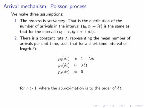
We make three assumptions:
1. The process is stationary. That is the distribution of thenumber of arrivals in the interval (t0, t0 + δt) is the same asthat for the interval (t0 + τ, t0 + τ + δt).
2. There is a constant rate λ, representing the mean number ofarrivals per unit time, such that for a short time interval oflength δt
p0(δt) ≈ 1− λδtp1(δt) ≈ λδt
pn(δt) ≈ 0
for n > 1, where the approximation is to the order of δt.
3. The numbers of arrivals in non-overlapping time intervals areindependent.

Arrival mechanism: Poisson process
We make three assumptions:
1. The process is stationary. That is the distribution of thenumber of arrivals in the interval (t0, t0 + δt) is the same asthat for the interval (t0 + τ, t0 + τ + δt).
2. There is a constant rate λ, representing the mean number ofarrivals per unit time, such that for a short time interval oflength δt
p0(δt) ≈ 1− λδtp1(δt) ≈ λδt
pn(δt) ≈ 0
for n > 1, where the approximation is to the order of δt.
3. The numbers of arrivals in non-overlapping time intervals areindependent.

Arrival mechanism: Poisson process
As an approximation, imagine dividing time up into sections, eachof length δt. Suppose that the probability that an arrival occurs ina particular section is λδt. In the time interval (0, t) there are t/δtsections. The number of sections with events in them has abinomial distribution and the probability of j events in (0, t) is
pj ≈(
t/δtj
)(λδt)j(1− λδt)t/δt−j
≈(
t/δtj
)(λδt
1− λδt
)j
(1− λδt)t/δt
≈ λj
j!t(t − δt)(t − 2δt) · · · (t − {j − 1}δt)(1− λδt)t/δt−j

Arrival mechanism: Poisson process
It is easily shown that
pj →exp(−λt)(λt)j
j!
as δt → 0.Thus N(t), the number of arrivals in the time interval (0, t), has aPoisson distribution with mean λt.

Arrival mechanism: Poisson process
We can prove formally that the number of arrivals in a timeinterval of length t has a Poisson distribution with mean λt.If this number is N(t) then
Pr{N(t) = j} =e−λt(λt)j
j!
for j = 0, 1, 2, . . . .

Arrival mechanism: Time till next arrival
I Consider the waiting time, T , till the next arrival.
I Suppose we start waiting at time 0. Here 0 may be a fixedpoint, the time of a previous arrival or whatever. It does notmatter.
I The probability that the arrival has not happened by time t is
Pr{N(t) = 0} = exp(−λt).
This is the probability that the waiting time is at least t.
I Thus the distribution function of T , that is the probabilitythat T < t, is
FT (t) = 1− exp(−λt).
I This is the distribution function of an exponential distributionwith parameter λ.

Distribution function of inter-arrival time
0 10 20 30 40 50
0.0
0.2
0.4
0.6
0.8
1.0
t
F((t))

Probability density functionIf a continuous random variable T has distribution function FT (t)then
fT (t) =d
dtFT (t)
is called the probability density function (or pdf) of T .Note that ∫ ∞
−∞fT (t) dt = 1
— the total probability.For our exponential distribution
FT (t) = 1− exp(−λt)
sofT (t) = λ exp(−λt)
(0 < t <∞).

Probability density function of inter-arrival time
0 10 20 30 40 50
0.00
0.04
0.08
t
f((t))

Example: Road vehicle headways
The times of arrivals of motor vehicles passing a point in ChesterRoad, Sunderland going East.
12.40 3, 6, 9,15,24,28,3012.41 7,12,14,16,21,24,30,5012.42 9,22,28,46,5312.43 22,25,35,38,5812.44 2, 5, 8,10,14,17,27,30,4512.45 3,4612.46 13,42,5112.47 0, 9,11,18,23,26,39,51
.............................
12.59 2,31,34,38,54,59
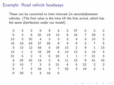
Example: Road vehicle headways
These can be converted to time intervals (in seconds)betweenvehicles. (The first value is the time till the first arrival, which hasthe same distribution under our model).
3 3 3 6 9 4 2 37 5 2 25 3 6 20 19 13 6 18 7 29 310 3 20 4 3 3 2 4 3 10 315 18 43 27 29 9 9 9 2 7 53 13 12 44 4 16 13 2 9 1 1312 1 2 16 26 4 13 13 4 14 331 5 2 5 5 20 1 1 7 21 34 25 22 14 2 4 11 15 8 41 183 10 7 3 5 21 6 5 22 2 25 7 3 24 3 7 32 3 19 2 16 29 3 4 16 5

Example: Road vehicle headways
Histogram of Headway
Headway
Den
sity
0 10 20 30 40
0.00
0.04
0.08
Time to second arrival
I The second arrival has not occurred before time t if N(t) < 2.
I Now
Pr{N(t) < 2} = Pr{N(t) = 0}+Pr{N(t) = 1} = e−λt+λte−λt
I Hence the distribution function is
F2(t) = 1− (1 + λt)e−λt
I Hence the probability density function is
f2(t) =d
dtF2(t)
= λ(1 + λt)e−λt − λe−λt
= λ2te−λt
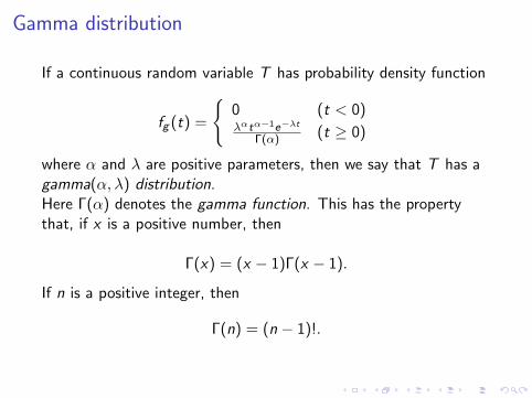
Gamma distribution
If a continuous random variable T has probability density function
fg (t) =
{0 (t < 0)λαtα−1e−λt
Γ(α) (t ≥ 0)
where α and λ are positive parameters, then we say that T has agamma(α, λ) distribution.Here Γ(α) denotes the gamma function. This has the propertythat, if x is a positive number, then
Γ(x) = (x − 1)Γ(x − 1).
If n is a positive integer, then
Γ(n) = (n − 1)!.

Gamma distribution
Gamma pdf:
fg (t) =λαtα−1e−λt
Γ(α)
The time to the second arrival has pdf
f2(t) =λ2t2−1e−λt
1!=λ2t2−1e−λt
Γ(2).
So this is a gamma(2, λ) distribution.Notice that an exponential(λ) distribution is a gamma(1, λ)distribution.
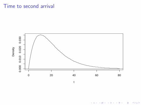
Time to second arrival
0 20 40 60 80
0.00
00.
010
0.02
00.
030
t
Den
sity

Mean of a continuous random variable
A continuous random variable X has pdf fX (x).Its mean or expectation (if it exists) is
E(X ) =
∫ ∞−∞
x fX (x) dx .
Similarly, if g(X ) is some function of X , then the expectation ofg(X ) is
E[g(X )] =
∫ ∞−∞
g(x) fX (x) dx .

Means: Example 1
T ∼ exponential(λ)
E(T ) =
∫ ∞0
tλe−λt dt
= [−te−λt ]∞0 +
∫ ∞0
e−λt dt
=
[− 1
λe−λt
]∞0
=1
λ

Means: Example 2
T ∼ gamma(α, λ)
E(T ) =
∫ ∞0
tλαtα−1e−λt
Γ(α)dt
=
∫ ∞0
λαtα+1−1e−λt
Γ(α)dt
=Γ(α + 1)
Γ(α)
1
λ
∫ ∞0
λα+1tα+1−1e−λt
Γ(α + 1)dt
=Γ(α + 1)
Γ(α)
1
λ
=α
λ
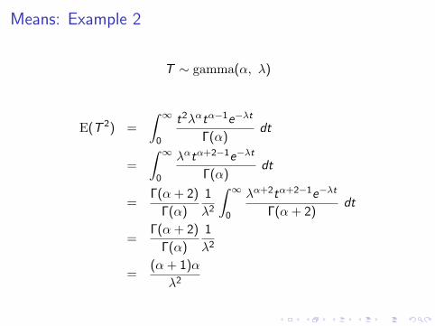
Means: Example 2
T ∼ gamma(α, λ)
E(T 2) =
∫ ∞0
t2λαtα−1e−λt
Γ(α)dt
=
∫ ∞0
λαtα+2−1e−λt
Γ(α)dt
=Γ(α + 2)
Γ(α)
1
λ2
∫ ∞0
λα+2tα+2−1e−λt
Γ(α + 2)dt
=Γ(α + 2)
Γ(α)
1
λ2
=(α + 1)α
λ2

Variance of a random variable
The variance of a quantitative random variable X (if it exists) is
Var(X ) = E{
[X − E(X )]2}
= E{X 2 − 2XE(X ) + [E(X )]2
}= E(X 2)− 2E(X )E(X ) + [E(X )]2
= E(X 2)− [E(X )]2

Variance: Example
T ∼ gamma(α, λ)
I
E(T ) =α
λI
E(T 2) =(α + 1)α
λ2
I So
Var(T ) =(α + 1)α
λ2−{αλ
}2=
α
λ2

Variance: Example
T ∼ gamma(α, λ)
I
E(T ) =α
λ
I
E(T 2) =(α + 1)α
λ2
I So
Var(T ) =(α + 1)α
λ2−{αλ
}2=
α
λ2

Variance: Example
T ∼ gamma(α, λ)
I
E(T ) =α
λI
E(T 2) =(α + 1)α
λ2
I So
Var(T ) =(α + 1)α
λ2−{αλ
}2=
α
λ2

Variance: Example
T ∼ gamma(α, λ)
I
E(T ) =α
λI
E(T 2) =(α + 1)α
λ2
I So
Var(T ) =(α + 1)α
λ2−{αλ
}2=
α
λ2

Normal distribution
I The normal distribution, sometimes called the Gaussiandistribution is very important in probability and statistics. It isa continuous distribution.
I It has two parameters, the mean and the variance, oftenwritten µ, σ2. If X has a normal distribution with mean µ andvariance σ2 we write
X ∼ N(µ, σ2
The range of X is −∞ < X <∞.I The probability density function is
1√2πσ2
exp
[−1
2
(x − µσ
)2]
(−∞ < x <∞).
I The distribution function can not be written explicitly.

Normal distribution
I The normal distribution, sometimes called the Gaussiandistribution is very important in probability and statistics. It isa continuous distribution.
I It has two parameters, the mean and the variance, oftenwritten µ, σ2. If X has a normal distribution with mean µ andvariance σ2 we write
X ∼ N(µ, σ2
The range of X is −∞ < X <∞.
I The probability density function is
1√2πσ2
exp
[−1
2
(x − µσ
)2]
(−∞ < x <∞).
I The distribution function can not be written explicitly.

Normal distribution
I The normal distribution, sometimes called the Gaussiandistribution is very important in probability and statistics. It isa continuous distribution.
I It has two parameters, the mean and the variance, oftenwritten µ, σ2. If X has a normal distribution with mean µ andvariance σ2 we write
X ∼ N(µ, σ2
The range of X is −∞ < X <∞.I The probability density function is
1√2πσ2
exp
[−1
2
(x − µσ
)2]
(−∞ < x <∞).
I The distribution function can not be written explicitly.

Normal distribution
I The normal distribution, sometimes called the Gaussiandistribution is very important in probability and statistics. It isa continuous distribution.
I It has two parameters, the mean and the variance, oftenwritten µ, σ2. If X has a normal distribution with mean µ andvariance σ2 we write
X ∼ N(µ, σ2
The range of X is −∞ < X <∞.I The probability density function is
1√2πσ2
exp
[−1
2
(x − µσ
)2]
(−∞ < x <∞).
I The distribution function can not be written explicitly.

Normal distribution
x
f(x)
4 12 20
0.00
0.06
xF(x
)
4 12 20
0.0
0.5
1.0
Probability density function f (x) and distribution function F (x) fora normal distribution with mean µ = 12 and variance σ2 = 16.

The standard normal distribution
If µ = 0 and σ2 = 1 we have a standard normal distribution. If Zhas a standard normal distribution we write Z ∼ N(0, 1).
I Probability density function:
φ(z) =1√2π
e−z2
2
I Distribution function:
Φ(z) =
∫ z
−∞φ(u) du

The lognormal distribution
I Sometimes a variable does not have a normal distribution butsome transformation of the variable does.
I For example, if X must be positive, eg a service time, thenperhaps ln(X ) has a normal distribution.
0 < X <∞ ⇔ −∞ < ln(X ) <∞
I If Y ∼ N(µ, σ2) and X = eY (so Y = ln(X )) then we saythat X has a lognormal(µ, σ2) distribution,X ∼ lognormal(µ, σ2).

The lognormal distribution
0 20 40 60
0.00
0.01
0.02
0.03
x
Den
sity
Probability density function for a lognormal distribution with µ = 3and σ2 = 0.49 (σ = 0.7).

The lognormal distribution
If X ∼ lognormal(µ, σ2) what is the mean of X?If X ∼ lognormal(µ, σ2) and Y = ln(X ) then E(X ) = E(eY ).Hence
E(X ) = E(eY ) =
∫ ∞−∞
ey (2πσ2)−1/2 exp
{− 1
2σ2(y − µ)2
}dy
=
∫ ∞−∞
(2πσ2)−1/2 exp
{y − 1
2σ2(y − µ)2
}dy

The lognormal distribution
y − 1
2σ2(y − µ)2 = − 1
2σ2[y2 − 2µy − 2σ2y + µ2]
= − 1
2σ2[y2 − 2(µ+ σ2)y + (µ+ σ2)2
−(µ+ σ2)2 + µ2]
= − 1
2σ2[{y − (µ+ σ2)}2 − (µ+ σ2)2 + µ2]
= − 1
2σ2[{y − (µ+ σ2)}2 − 2µσ2 − σ4]
= − 1
2σ2(y − θ)2 + µ+
σ2
2
where θ = µ+ σ2.

The lognormal distribution
Hence
E(X ) =
∫ ∞−∞
(2πσ2)−1/2 exp
{− 1
2σ2(y − θ)2
}dy eµ+σ2/2
= eµ+σ2/2

Estimation: Method of moments
I A simple way to estimate the values of parameters of adistribution if we have data is to equate sample moments(mean, variance) with theoretical moments and solve.
I Suppose we have n = 50 independent observations y1, . . . , y50
from N(µ, σ2):
5.82 3.96 3.57 5.00 ...... 5.32 5.95 5.64 6.66 3.33
I Sample mean:
y =1
n
n∑i=1
yi =268.3
50= 5.366.
I We estimate µ with µ = y = 5.366.
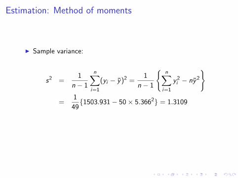
Estimation: Method of moments
I Sample variance:
s2 =1
n − 1
n∑i=1
(yi − y)2 =1
n − 1
{n∑
i=1
y2i − ny2
}
=1
49{1503.931− 50× 5.3662} = 1.3109
I We estimate σ2 with σ2 = s2 = 1.3109 and estimate thestandard deviation σ with s =
√s2 = 1.1449.

Estimation: Method of moments
I Sample variance:
s2 =1
n − 1
n∑i=1
(yi − y)2 =1
n − 1
{n∑
i=1
y2i − ny2
}
=1
49{1503.931− 50× 5.3662} = 1.3109
I We estimate σ2 with σ2 = s2 = 1.3109 and estimate thestandard deviation σ with s =
√s2 = 1.1449.
Estimation: Lognormal distribution
In the case of data from a lognormal distribution we can saimplytake logs of the data and then proceed as for a normal distribution.Eg: X1, . . . ,X50 ∼ lognormal(µ, σ2).Data: 336.97, 52.46, 35.52, 148.41, . . .Take logs: 5.82, 3.96, 3.57, 5.00, . . . as before.

Simulation
I One way to investigate stochastic system behaviour is tosimulate.
I Quicker and cheaper than experimenting on the real thing!
I Generate artificial pseudo-random inter-arrival times andservice times.
I Build up the events and see what happens.
I Possibly repeat many times.
I Actually more useful in more complicated systems.

Simulation: Example
As an example, consider use of a computer network.
I Users log on as a Poisson process. Inter-arrival times areindependent exponential(λ) variables.Choose λ = 0.1. So mean inter-arrival time is 10.
I Service times: Users stay logged on for random lengths oftime, eg lognormal(µ, σ2).Choose µ = 3.5, σ2 = 1.0 so µ+ σ2/2 = 4.0 and the meanservice time is e4 = 54.6.
I We assume that there is unlimited capacity.
I Let us start the simulation with an empty system.
I Generate inter-arrival and service times by computer. (In thecase of lognormal service times we might generate normalrandom variables and then exponentiate).

Simulation: Inter-arrival and service times
UserInter-arrivaltime
Arrivaltime
Servicetime
Serviceends
1 15.7 44.22 10.4 24.93 3.9 83.04 12.7 19.25 7.8 41.86 1.0 16.97 28.2 37.78 10.4 23.19 13.4 83.8
10 0.3 49.611 3.5 11.312 7.7 6.5

Simulation: Service start and end times
UserInter-arrivaltime
Arrivaltime
Servicetime
Serviceends
1 15.7 15.7 44.2 59.92 10.4 26.1 24.9 51.03 3.9 30.0 83.0 113.04 12.7 42.7 19.2 61.95 7.8 50.5 41.8 92.36 1.0 51.5 16.9 68.47 28.2 79.7 37.7 117.48 10.4 90.1 23.1 113.29 13.4 103.5 83.8 187.3
10 0.3 103.8 49.6 153.411 3.5 107.3 11.3 118.612 7.7 115.0 6.5 121.5

Simulation: Events and user numbers
Event Time ChangeNumber ofusers
0.0 0 01 15.7 1 12 26.1 1 23 30.0 1 34 42.7 1 45 50.5 1 56 51.0 -1 47 51.5 1 58 59.9 -1 49 61.9 -1 3
10 68.4 -1 211 79.7 1 3

Simulation: Graph
0 50 100 150
02
46
8
Time (Minutess)
Use
rs

Simulation: Second run
0 50 100 150 200 250
02
46
8
Time (Minutess)
Use
rs

Simulation: Change to µ = 5
0 50 100 150
02
46
810
Time (Minutess)
Use
rs


![08 Queueing Models.ppt [Kompatibilitätsmodus] ... KeyelementsofqueueingsystemsKey elements of queueing systems ... • Customer is pendingwhen the customer is outside the queueing](https://static.fdocuments.in/doc/165x107/5b236bc17f8b9a92298b6c18/08-queueing-kompatibilitaetsmodus-keyelementsofqueueingsystemskey-elements.jpg)