Partitioning and Divide-and-Conquer Strategies · 108 Partitioning and Divide-and-Conquer...

107

Partitioning and Divide-and-ConquerStrategies

In this chapter, we explore two of the most fundamental techniques in parallel program-ming, calledpartitioning anddivide and conquer, which are related. In partitioning, theproblem is simply divided into separate parts and each part is computed separately. Divideand conquer usually applies partitioning in a recursive manner by continually dividing theproblem into smaller and smaller parts before solving the smaller parts and combining theresults. First, we will review the technique of partitioning. Then we discuss recursivedivide-and-conquer methods. Next, we outline some typical problems that can be solvedwith these approaches. As usual, we have a selection of scientific/numerical and real-lifeproblems at the end of the chapter.

4.1 PARTITIONING

4.1.1 Partitioning Strategies

Partitioning simply divides the problem into parts. It is the basis of all parallel program-ming, in one form or another. The embarrassingly parallel problems in the last chapter usedpartitioning. Most partitioning formulations, however, require the results of the parts to becombined to obtain the desired result. Partitioning can be applied to the program data (thatis, to dividing the data and operating upon the divided data concurrently). This is calleddata partitioning or domain decomposition. Partitioning can also be applied to thefunctions of a program (that is, dividing the program into independent functions andexecuting the functions concurrently). This isfunctional decomposition. The idea of per-

4Chapter

108 Partitioning and Divide-and-Conquer Strategies Chap. 4

forming a task by dividing it into a number of smaller tasks that when completed willcomplete the overall task is, of course, well known and can be applied in many situations,whether the smaller tasks operate upon parts of the data or are separate concurrent func-tions.

It is much less common to find concurrent functions in a problem, but data partition-ing is a main strategy for parallel programming. To take a really simple data partitioningexample, suppose a sequence of numbers,x0 … xn−1, are to be added. This is a problemrecurring in the text to demonstrate a concept; clearly unless there were a huge sequence ofnumbers, a parallel solution would not be worthwhile. However, the approach can be usedfor more realistic applications involving complex calculations on large databases.

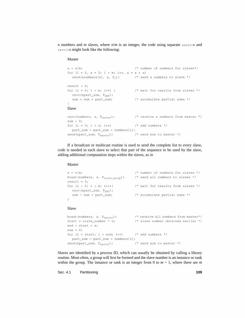
We might consider dividing the sequence intom parts ofn/m numbers each, (x0 …x(n/m)−1), (xn/m … x(2n/m)−1), …, (x(m−1)n/m … xn−1), at which pointm processors (or pro-cesses) can each add one sequence independently to create partial sums. Them partial sumsneed to be added together to form the final sum. Figure 4.1 shows the arrangement in whicha single processor adds them partial sums. Notice that each processor requires access to thenumbers it has to accumulate. In a message-passing system, the numbers would need to bepassed to the processors individually. (In a shared memory system, each processor couldaccess those numbers it wanted from the shared memory, and in this respect, a sharedmemory system would clearly be more convenient for this and similar problems.)

The parallel code for this example is straightforward. For a simple master-slaveapproach, the numbers are first sent from the master processor to slave processors. Theslave processors add their numbers, operating independently and concurrently. Next, thepartial sums are sent from the slaves to the master processor. Finally, the master processoradds the partial sums to form the result. Often, we talk of processes rather than processorsfor code sequences, where one process is best mapped onto one processor.

It is a moot point whether broadcasting the whole list of numbers to every slave oronly sending the specific numbers to each slave is best, since in both cases all numbers mustbe sent from the master. The specifics of the broadcast mechanism would need to be knownin order to decide on the relative merits of that mechanism. A broadcast will have a singlestartup time rather than separate startup times when using multiple send routines and maybe preferable.

First, we will send the specific numbers to each slave using individualsend() s. Given

Figure 4.1 Partitioning a sequence of numbers into parts and adding the parts.

Sum

x0 … x(n/m)−1 xn/m … x(2n/m)−1 x(m−1)n/m… xn−1…

Partial sums

+ +

+

+

Sec. 4.1 Partitioning 109

n numbers andm slaves, wheren/m is an integer, the code using separatesend() s andrecv() s might look like the following:

Master

s = n/m; /* number of numbers for slaves*/

for (i = 0, x = 0; i < m; i++, x = x + s)

send(&numbers[x], s, P i ); /* send s numbers to slave */

result = 0;

for (i = 0; i < m; i++) { /* wait for results from slaves */

recv(&part_sum, P ANY);

sum = sum + part_sum; /* accumulate partial sums */

}

Slave

recv(numbers, s, P master ); /* receive s numbers from master */

sum = 0;

for (i = 0; i < s; i++) /* add numbers */

part_sum = part_sum + numbers[i];

send(&part_sum, P master ); /* send sum to master */

If a broadcast or multicast routine is used to send the complete list to every slave,code is needed in each slave to select that part of the sequence to be used by the slave,adding additional computation steps within the slaves, as in

Master

s = n/m; /* number of numbers for slaves */

bcast(numbers, s, P slave_group ); /* send all numbers to slaves */

result = 0;

for (i = 0; i < m; i++){ /* wait for results from slaves */

recv(&part_sum, P ANY);

sum = sum + part_sum; /* accumulate partial sums */

}

Slave

bcast(numbers, s, P master ); /* receive all numbers from master*/

start = slave_number * s; /* slave number obtained earlier */

end = start + s;

sum = 0;

for (i = start; i < end; i++) /* add numbers */

part_sum = part_sum + numbers[i];

send(&part_sum, P master ); /* send sum to master */

Slaves are identified by a process ID, which can usually be obtained by calling a libraryroutine. Most often, a group will first be formed and the slave number is an instance or rankwithin the group. The instance or rank is an integer from 0 tom − 1, where there arem


processes in the group. MPI requires communicators to be established, and processes haverank within a communicator, as described in Chapter 2. Groups can be associated withincommunicators, and processes have a rank within groups. PVM has the concept of groups,but a unique process ID can also be obtained from thePVM_spawn() routine when theprocess is created, which could be used for very simple programs. (PVM process IDs arenot small consecutive integers; they are similar to normal UNIX process IDs.)

If scatter and reduce routines are available,1 the code could be

Master

s = n/m; /* number of numbers */

scatter(numbers,&s,P group ,root=master); /* send numbers to slaves */

reduce_add(&sum,&s,P group ,root=master); /* results from slaves */

Slave

scatter(numbers,&s,P group ,root=master); /* receive s numbers */

reduce_add(&part_sum,&s,P group ,root=master);/* send sum to master */

Remember, a simple pseudocode is used throughout. Scatter and reduce (and gather whenused) have many additional parameters in practice to include both source and destination(see Chapter 2, Section 2.2.4). Normally, the operation of a reduce routine will be specifiedas a parameter and not as part of the routine name as here. Using a parameter does allowdifferent operations to be selected easily. Code will also be needed to establish the group ofprocesses participating in the broadcast, scatter, and reduce.

Although we are adding numbers, many other operations could be performed instead.For example, the maximum number of the group could be found and passed back to themaster in order for the master to find the maximum number of all those passed back to it.Similarly, the number of occurrences of a number (or character, or a string of characters)can be found in groups and passed back to the master.

Analysis. The sequential computation requiresn − 1 additions with a time com-plexity ofΟ(n). In the parallel implementation, the total number of processes used ism + 1.Our analyses throughout separate communication and computation. It is easier to visualizeif we also separate the actions into distinct phases. As with many problems, there is a com-munication phase followed by a computation phase, and these phases are repeated.

Phase 1 — Communication. First, we need to consider the communication aspectof the m slave processes reading theirn/m numbers. Using individual send and receiveroutines requires a communication time of

tcomm1 = m(tstartup + (n/m)tdata)

wheretstartup is the constant time portion of the transmission andtdata is the time to transmitone data word. Using scatter might reduce the number of startup times; i.e.,

tcomm1 = tstartup + ntdata

1MPI has these, but PVM version 3 only has reduce.


depending upon the implementation of scatter. In any event, the time complexity is stillΟ(n).

Phase 2 — Computation. Next, we need to estimate the number of computationalsteps. The slave processes each addn/m numbers together, requiringn/m − 1 additions.Since allm slave processes are operating together, we can consider all the partial sumsobtained in then/m − 1 steps. Hence, the parallel computation time of this phase is

tcomp1 = n/m − 1

Phase 3 — Communication. Returning partial results using individual send andreceive routines has a communication time of

tcomm2 = m(tstartup + tdata)

Using gather and reduce has:

tcomm2 = tstartup + mtdata

Phase 4 — Computation. For the final accumulation, the master has to add thempartial sums, which requiresm − 1 steps:

tcomp2 = m − 1

Overall. The overall execution time for the problem (with gather and scatter) is

tp = (tcomm1 + tcomm2) + (tcomp1 + tcomp2)

= (m(tstartup + (n/m)tdata) +tstartup + mtdata) + (n/m − 1 + m − 1)

= (m + 1)tstartup + (n + m)tdata + m + n/m

or

tp = O(n + m)

We see that the parallel time complexity is worse than the sequential time complexity ofΟ(n). Of course, if we consider only the computation aspect, the parallel formulation isbetter than the sequential formulation. Ignoring the communication aspect, the speedupfactor,S, is given by

The speedup tends tom for largen. However, for smallern, the speedup will be quite lowand worsen for an increasing number of slaves, because them slaves are idle during thesecond phase forming the final result.

Ideally, we want all the processes to be active all of the time, which cannot beachieved with this formulation of the problem. However, another formulation is helpful andis applicable to a very wide range of problems — namely, the divide-and-conquer approach.

4.1.2 Divide and Conquer

The divide-and-conquer approach is characterized by dividing a problem into subproblemsthat are of the same form as the larger problem. Further divisions into still smaller sub-

Ststp---- n 1–

n m⁄ m 2–+-------------------------------= =


problems are usually done by recursion, a method well known to sequential programmers.The recursive method will continually divide a problem until the tasks cannot be brokendown into smaller parts. Then the very simple tasks are performed and results combined,with the combining continued with larger and larger tasks. JáJá (1992) differentiatesbetween when the main work is in dividing the problem and when the main work iscombining the results (c.f., quicksort with mergesort). He categorizes the method as divideand conquer when the main work is combining the results, and categorizes the method aspartitioning when the main work is dividing the problem. We will not make that distinctionbut will use the termdivide and conquer anytime the partitioning is continued on smallerand smaller problems.

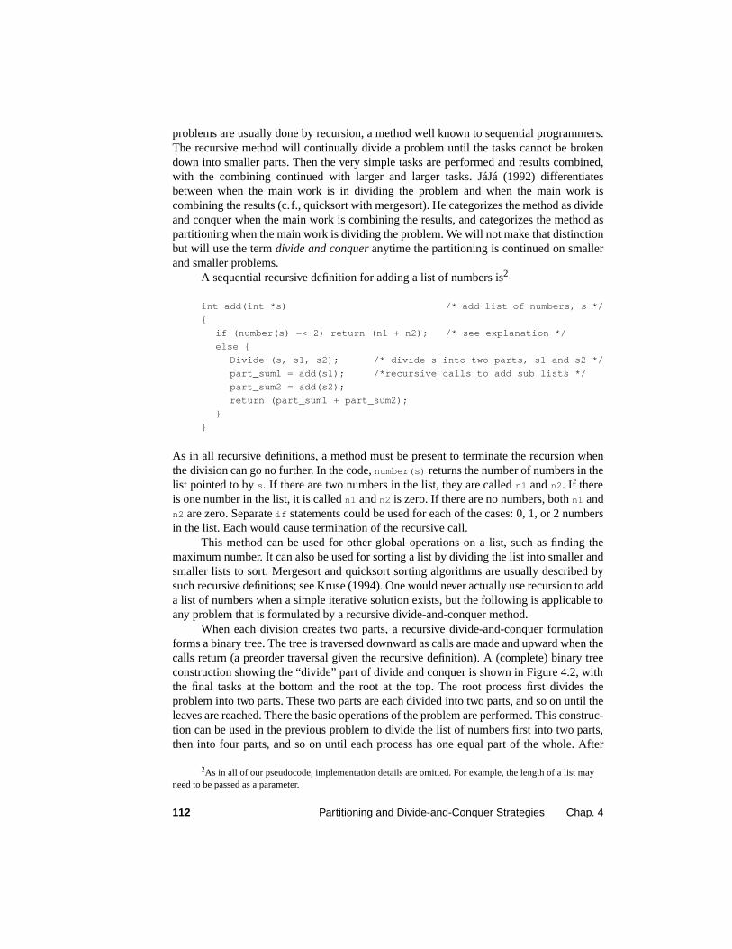
A sequential recursive definition for adding a list of numbers is2

int add(int *s) /* add list of numbers, s */

{

if (number(s) =< 2) return (n1 + n2); /* see explanation */

else {

Divide (s, s1, s2); /* divide s into two parts, s1 and s2 */

part_sum1 = add(s1); /*recursive calls to add sub lists */

part_sum2 = add(s2);

return (part_sum1 + part_sum2);

}

}

As in all recursive definitions, a method must be present to terminate the recursion whenthe division can go no further. In the code,number(s) returns the number of numbers in thelist pointed to bys. If there are two numbers in the list, they are calledn1 andn2. If thereis one number in the list, it is calledn1 andn2 is zero. If there are no numbers, bothn1 andn2 are zero. Separateif statements could be used for each of the cases: 0, 1, or 2 numbersin the list. Each would cause termination of the recursive call.

This method can be used for other global operations on a list, such as finding themaximum number. It can also be used for sorting a list by dividing the list into smaller andsmaller lists to sort. Mergesort and quicksort sorting algorithms are usually described bysuch recursive definitions; see Kruse (1994). One would never actually use recursion to adda list of numbers when a simple iterative solution exists, but the following is applicable toany problem that is formulated by a recursive divide-and-conquer method.

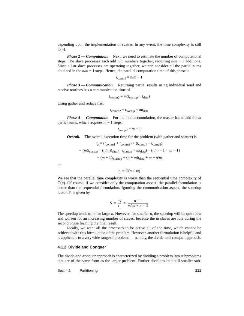
When each division creates two parts, a recursive divide-and-conquer formulationforms a binary tree. The tree is traversed downward as calls are made and upward when thecalls return (a preorder traversal given the recursive definition). A (complete) binary treeconstruction showing the “divide” part of divide and conquer is shown in Figure 4.2, withthe final tasks at the bottom and the root at the top. The root process first divides theproblem into two parts. These two parts are each divided into two parts, and so on until theleaves are reached. There the basic operations of the problem are performed. This construc-tion can be used in the previous problem to divide the list of numbers first into two parts,then into four parts, and so on until each process has one equal part of the whole. After

2As in all of our pseudocode, implementation details are omitted. For example, the length of a list mayneed to be passed as a parameter.


adding pairs at the bottom of the tree, the accumulation occurs in a reverse tree construc-tion.

Figure 4.2 shows a complete binary tree; that is, a perfectly balanced tree with allbottom nodes at the same level. This occurs if the task can be divided into a number of partsthat is a power of 2. If not a power of 2, one or more bottom nodes will be at one level higherthan the others. For convenience, we will assume that the task can be divided into a numberof parts that is a power of 2, unless otherwise stated.

Parallel Implementation. In a sequential implementation, only one node of thetree can be visited at a time. A parallel solution offers the prospect of traversing severalparts of the tree simultaneously. Once a division is made into two parts, both parts can beprocessed simultaneously. Though a recursive parallel solution could be formulated, it iseasier to visualize it without recursion. The key is realizing that the construction is a tree.One could simply assign one processor to each node in the tree. That would ultimatelyrequire 2m+1 − 1 processors to divide the tasks into 2m parts. Each processor would only beactive at one level in the tree, leading to a very inefficient solution. (Problem 4-5 exploresthis method.)

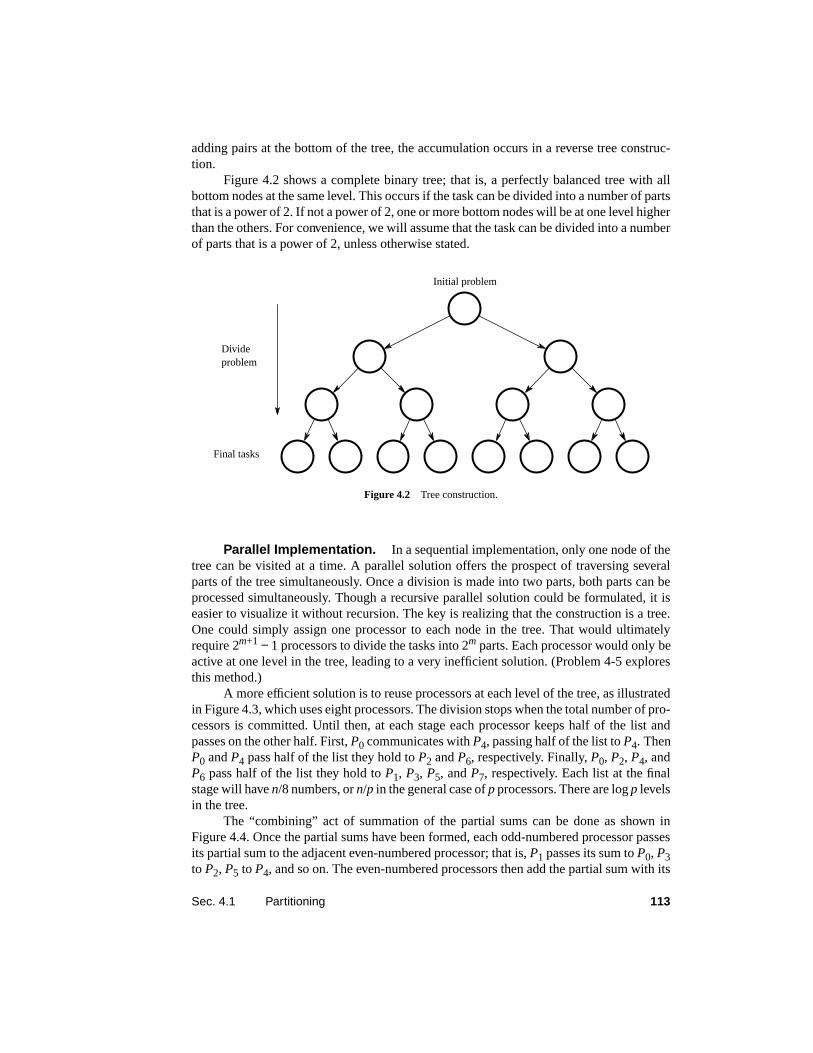
A more efficient solution is to reuse processors at each level of the tree, as illustratedin Figure 4.3, which uses eight processors. The division stops when the total number of pro-cessors is committed. Until then, at each stage each processor keeps half of the list andpasses on the other half. First,P0 communicates withP4, passing half of the list toP4. ThenP0 andP4 pass half of the list they hold toP2 andP6, respectively. Finally,P0, P2, P4, andP6 pass half of the list they hold toP1, P3, P5, andP7, respectively. Each list at the finalstage will haven/8 numbers, orn/p in the general case ofp processors. There are logp levelsin the tree.

The “combining” act of summation of the partial sums can be done as shown inFigure 4.4. Once the partial sums have been formed, each odd-numbered processor passesits partial sum to the adjacent even-numbered processor; that is,P1 passes its sum toP0, P3to P2, P5 to P4, and so on. The even-numbered processors then add the partial sum with its

Figure 4.2 Tree construction.

Initial problem

Divide

Final tasks

problem


own partial sum and pass the result onward, as shown. This continues untilP0 has the finalresult.

We can see that these constructions are the same as the binary hypercube broadcastand gather algorithms described in Chapter 2, Section 2.3.3. The constructions would maponto a hypercube perfectly but are also applicable to other systems. As with the hypercubebroadcast/gather algorithms, processors that are to communicate with other processors canbe found from their binary addresses. Processors communicate with processors whoseaddresses differ in one bit, starting with the most significant bit for the division phase andwith the least significant bit for the combining phase (see Chapter 2, Section 2.3.3).

Figure 4.3 Dividing a list into parts.

P0 P1 P2 P3 P4 P5 P6 P7

P0

P0

P0 P2 P4 P6

P4

Original list

x0 xn−1

Figure 4.4 Partial summation.

P0 P1 P2 P3 P4 P5 P6 P7

P0

P0

P0 P2 P4 P6

P4

Final sum

x0 xn−1


Suppose we statically create eight processors (or processes) to add a list of numbers.The parallel code for processP0 might take the form

ProcessP0/* division phase */

divide(s1, s1, s2); /* divide s1 into two, s1 and s2 */

send(s2, P 4); /* send one part to another process */

divide(s1, s1, s2);

send(s2, P 2);

divide(s1, s1, s2);

send(s2, P 0};

part_sum = *s1; /* combining phase */

recv(&part_sum1, P 0);

part_sum = part_sum + part_sum1;





The code for processP4 might take the form

ProcessP4

recv(s1, P 0); /* division phase */

divide(s1, s1, s2);

send(s2, P 6);

divide(s1, s1, s2);

send(s2, P 5);

part_sum = *s1; /* combining phase */





send(&part_sum, P 0);

Similar sequences are required for the other processes.

Analysis. We shall assume thatn is a power of 2. The communication setup time,tstartup, is not included in the following for simplicity. It is left as an exercise to include thestartup time.

The division phase essentially only consists of communication if we assume thatdividing the list into two parts requires minimal computation. The combining phaserequires both computation and communication to add the partial sums received and pass onthe result.

Communication . There is a logarithmic number of steps in the division phase; i.e.,logp steps withp processes. The communication time for this phase is given by


wheretdata is the transmission time for one data word. The timetcomm1 is marginally betterthan a simple broadcast. The combining phase is similar, except only one data item is sentin each message (the partial sum); i.e.,

for a total communication time of

or a time complexity ofΟ(n) for constantp.

Computation. At the end of the divide phase, then/p numbers are added together.Then one addition occurs at each stage during the combining phase, leading to

again a time complexity ofΟ(n) for constantp. For largen and variablep, we getΟ(n/p).The total parallel execution time becomes

assuming thatp is a power of 2. The very best speedup we could expect with this methodis, of course,p when allp processors are computing their partial sums. The actual speedupwill be less than this due to the division and combining phases.

Clearly, another associative operator, such as subtraction, logical OR, logical AND,etc., can replace the addition operation in the previous example. The basic idea can also beapplied to evaluating arithmetic expressions where operands are connected with an arith-metic operator. The tree construction can also be used for operations such as searching. Inthis case, the information passed upward is a Boolean flag indicating whether or not thespecific item or condition has been found. The operation performed at each node is an ORoperation, as shown in Figure 4.5.

tcomm1n2---tdata

n4---tdata

n8---tdata … n

p---tdata+ + + +

n p 1–( )p

--------------------tdata= =

tcomm2 tdata plog=

tcomm tcomm1 tcomm2+n p 1–( )

p--------------------tdata tdata plog+= =

tcompnp--- plog+=

t pn p 1–( )

p--------------------tdata tdata plog n

p--- plog+ + +=

OR

OROR

Found/Not found

Figure 4.5 Part of a search tree.


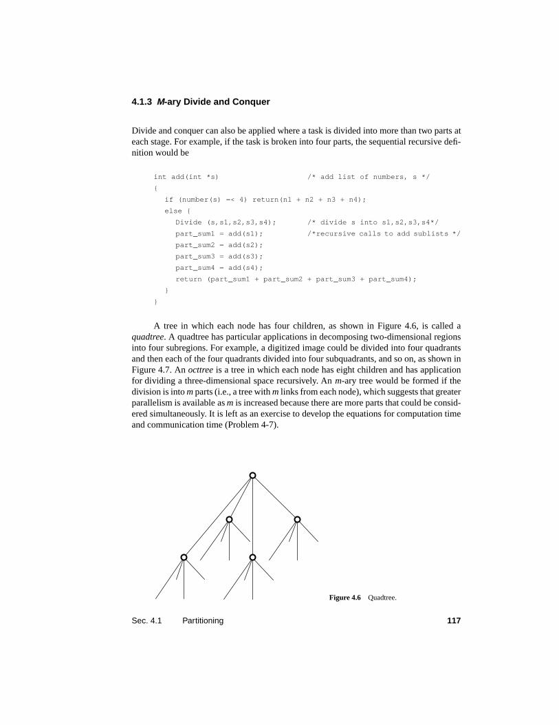
4.1.3 M-ary Divide and Conquer

Divide and conquer can also be applied where a task is divided into more than two parts ateach stage. For example, if the task is broken into four parts, the sequential recursive defi-nition would be

int add(int *s) /* add list of numbers, s */

{

if (number(s) =< 4) return(n1 + n2 + n3 + n4);

else {

Divide (s,s1,s2,s3,s4); /* divide s into s1,s2,s3,s4*/

part_sum1 = add(s1); /*recursive calls to add sublists */




return (part_sum1 + part_sum2 + part_sum3 + part_sum4);

}

}

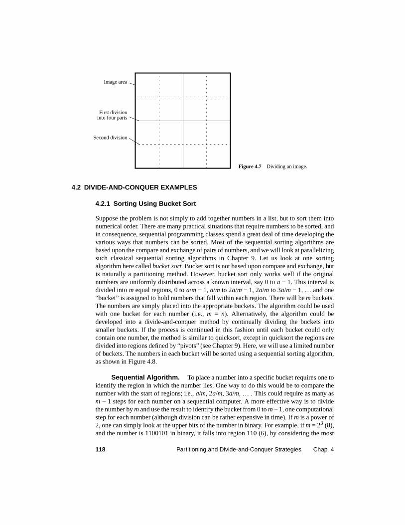
A tree in which each node has four children, as shown in Figure 4.6, is called aquadtree. A quadtree has particular applications in decomposing two-dimensional regionsinto four subregions. For example, a digitized image could be divided into four quadrantsand then each of the four quadrants divided into four subquadrants, and so on, as shown inFigure 4.7. Anocttree is a tree in which each node has eight children and has applicationfor dividing a three-dimensional space recursively. An m-ary tree would be formed if thedivision is intom parts (i.e., a tree withm links from each node), which suggests that greaterparallelism is available asm is increased because there are more parts that could be consid-ered simultaneously. It is left as an exercise to develop the equations for computation timeand communication time (Problem 4-7).

Figure 4.6 Quadtree.


4.2 DIVIDE-AND-CONQUER EXAMPLES

4.2.1 Sorting Using Bucket Sort

Suppose the problem is not simply to add together numbers in a list, but to sort them intonumerical order. There are many practical situations that require numbers to be sorted, andin consequence, sequential programming classes spend a great deal of time developing thevarious ways that numbers can be sorted. Most of the sequential sorting algorithms arebased upon the compare and exchange of pairs of numbers, and we will look at parallelizingsuch classical sequential sorting algorithms in Chapter 9. Let us look at one sortingalgorithm here calledbucket sort. Bucket sort is not based upon compare and exchange, butis naturally a partitioning method. However, bucket sort only works well if the originalnumbers are uniformly distributed across a known interval, say 0 toa − 1. This interval isdivided intom equal regions, 0 toa/m − 1, a/m to 2a/m − 1, 2a/m to 3a/m − 1, … and one“bucket” is assigned to hold numbers that fall within each region. There will bem buckets.The numbers are simply placed into the appropriate buckets. The algorithm could be usedwith one bucket for each number (i.e.,m = n). Alternatively, the algorithm could bedeveloped into a divide-and-conquer method by continually dividing the buckets intosmaller buckets. If the process is continued in this fashion until each bucket could onlycontain one number, the method is similar to quicksort, except in quicksort the regions aredivided into regions defined by “pivots” (see Chapter 9). Here, we will use a limited numberof buckets. The numbers in each bucket will be sorted using a sequential sorting algorithm,as shown in Figure 4.8.

Sequential Algorithm. To place a number into a specific bucket requires one toidentify the region in which the number lies. One way to do this would be to compare thenumber with the start of regions; i.e.,a/m, 2a/m, 3a/m, … . This could require as many asm − 1 steps for each number on a sequential computer. A more effective way is to dividethe number bym and use the result to identify the bucket from 0 tom− 1, one computationalstep for each number (although division can be rather expensive in time). Ifm is a power of2, one can simply look at the upper bits of the number in binary. For example, ifm = 23 (8),and the number is 1100101 in binary, it falls into region 110 (6), by considering the most

Image area

First division

Second division

into four parts

Figure 4.7 Dividing an image.

Sec. 4.2 Divide-and-Conquer Examples 119

significant three bits. In any event, let us assume that placing a number into a bucketrequires one step, and hence placing all the numbers requiresn steps. If the numbers areuniformly distributed, there should be aboutn/m numbers in each bucket.

Next, each bucket must be sorted. Sequential sorting algorithms such as quicksort ormergesort have a time complexity of Ο(nlogn) to sortn numbers (average time complexityfor quicksort). The lower bound on any compare and exchange sorting algorithm is aboutn logn comparisons (Aho, Hopcroft, and Ullman, 1974). Let us assume that the sequentialsorting algorithm actually requiresn logn comparisons, one comparison being regarded asone computational step. Thus, it will take (n/m)log(n/m) steps to sort then/m numbers ineach bucket using these sequential sorting algorithms. The sorted numbers must be concat-enated into the final sorted list. Let us assume that this concatenation requires no additionalsteps. Combining all the actions, the sequential time becomes

ts = n + m((n/m)log(n/m)) = n + n log(n/m) = Ο(n log(n/m))

If n = km, wherek is a constant, we get a time complexity of Ο(n). Notice that this is muchbetter than the lower bound for sequential compare and exchange sorting algorithms.However, it only applies when the numbers are well distributed.

Parallel Algorithm. Clearly, bucket sort can be parallelized by assigning oneprocessor for each bucket, which reduces the second term in the preceding equation to(n/p)log (n/p) for p processors (wherep = m). This implementation is illustrated in Figure4.9. In this version, each processor examines each of the numbers, so that a great deal ofwasted effort takes place. The implementation could be improved by having processorsactually remove numbers from the list into their buckets so that these numbers are notreconsidered by other processors.

We can further parallelize the algorithm by partitioning the sequence intom regions,one region for each processor. Each processor maintainsp “small” buckets and separatesthe numbers in its region into its own small buckets. These small buckets are then“emptied” into thep final buckets for sorting, which requires each processor to send onesmall bucket to each of the other processors (bucketi to processori). The overall algorithmis shown in Figure 4.10. Notice that this method is a simple partitioning method in whichthere is minimal work to create the partitions.

Unsorted numbers

Sorted numbers

Buckets

Figure 4.8 Bucket sort.

Sortcontentsof buckets

Merge lists


The following phases are needed:

1. Partition numbers.

2. Sort into small buckets.

3. Send to large buckets.

4. Sort large buckets.

Unsorted numbers

Sort

Figure 4.9 One parallel version of bucket sort.

Buckets

contentsof buckets

Merge lists

p processors

Sorted numbers

Unsorted numbers

Sort

Large

Figure 4.10 Parallel version of bucket sort.

Smallbuckets

Emptysmallbuckets

buckets

contentsof buckets

Merge lists

p processors

n/m numbers

Sorted numbers


Phase 1 — Computation and Communication.If we assumen computationalsteps to partitionn numbers intop regions, then the computation is

tcomp1 = n

After partitioning, thep partitions containingn/p numbers each are sent to the processes.Using a broadcast or scatter routine, the communication time is:

tcomm1 = tstartup + tdatan

including the communication startup time.

Phase 2 — Computation. To separate each partition ofn/p numbers intop smallbuckets requires the time

tcomp2 = n/p

Phase 3 — Communication. Next, the small buckets are distributed. (There is nocomputation in Phase 3.) Each small bucket will have aboutn/p2 numbers (assuminguniform distribution). Each process must send the contents ofp − 1 small buckets to otherprocesses (one bucket being held for its own large bucket). Since each process of thepprocesses must make this communication, we have

tcomm3 = p(p − 1)(tstartup + (n/p2)tdata)

if these communications cannot be overlapped in time and individual send() s are used.This is the upper bound on this phase of communication. The lower bound would occur ifall the communications could overlap, leading to

tcomm3 = (p − 1)(tstartup + (n/p2)tdata)

In essence, each processor must communicate with every other processor and an “all-to-all”mechanism would be appropriate. An “all-to-all” routine sends data from each process toevery other process and is illustrated in Figure 4.11. This type of routine is available in MPI(MPI_Alltoall() ), which we assume would be implemented more efficiently than usingindividual send() s andrecv() s. The “all-to-all” routine will actually transfer the rows ofan array to columns, as illustrated in Figure 4.12 (and hence transpose a matrix; see Chapter9, Section 9.2.3).

Phase 4 — Computation. In the final phase, the large buckets are sorted simulta-neously. Each large bucket contains aboutn/p numbers. Hence

tcomp4 = (n/p)log(n/p)

Overall. The overall run time including communication is

tp = tstartup + tdatan + n/p + (p − 1)(tstartup + (n/p2)tdata) +(n/p)log(n/p)

It is assumed that the numbers are uniformly distributed to obtain these formulas. If thenumbers are not uniformly distributed, some buckets would have more numbers than othersand sorting them would dominate the overall computation time. The worst-case scenariowould occur when all the numbers fell into one bucket!


4.2.2 Numerical Integration

Previously, we divided a problem and solved each subproblem. The problem was assumedto be divided into equal parts, and simple partitioning was employed. Sometimes simplepartitioning will not give the optimum solution, especially if the amount of work in eachpart is difficult to estimate. Bucket sort, for example, is only effective when each region hasapproximately the same number of numbers. Bucket sort can be modified to equalize thework, see Kumar et al. (1994).

A general divide-and-conquer technique divides the region continually into parts andlets some optimization function decide when certain regions are sufficiently divided. Let ustake a different example, numerical integration:

Send Receive

Send

Process 1 Processn − 1



0 n − 1 0 n − 1 0 n − 1 0 n − 1

Figure 4.11 “All-to-all” broadcast.

buffer buffer

buffer

A0,0 A0,1 A0,2 A0,3

A1,0 A1,1 A1,2 A1,3

A3,0 A3,1 A3,2 A3,3

A2,0 A2,1 A2,2 A2,3

A0,0 A1,0 A2,0 A3,0

A0,1 A1,1 A2,1 A3,1

A0,3 A1,3 A2,3 A3,3

A0,2 A1,2 A2,2 A3,2

P0

P1

P2

P3

“All-to-all”

Figure 4.12 Effect of “all-to-all” on anarray.

I f x( ) xda

b∫=


To integrate this function (i.e., to compute the “area under the curve”), we can divide thearea into separate parts, each of which can be calculated by a separate process. Each regioncould be calculated using an approximation given by rectangles, as shown in Figure 4.13,wheref(p) andf(q) are the heights of the two edges of a rectangular region andδ is the width(the interval). The complete integral can be approximated by the summation of the rectan-gular regions froma tob. A better approximation can be obtained by aligning the rectanglesso that the upper midpoint of each rectangle intersects with the function, as shown in Figure4.14. This construction has the advantage that the errors on each side of the midpoint endtend to cancel. Another more obvious construction is to use the actual intersections of thevertical lines with the function to create trapezoidal regions, as shown in Figure 4.15. Eachregion is now calculated as 1/2(f(p) + f(q))δ. Such approximate numerical methods forcomputing a definite integral using a linear combination of values are calledquadraturemethods.

Static Assignment. Let us consider thetrapezoidal method. Prior to the start ofthe computation, one process is statically assigned to be responsible for computing eachregion. By making the interval smaller, we come closer to attaining the exact solution.

Since each calculation is of the same form, the SPMD (single program multiple data)model is appropriate. Suppose we were to sum the area fromx = a tox = b usingp processesnumbered 0 top − 1. The size of the region for each process is (b − a)/p. To calculate thearea in the described manner, a section of SPMD pseudocode could be

Figure 4.13 Numerical integration usingrectangles.

f(q)f(p)

δ

f(x)

xp qa b

f(q)f(p)

δFigure 4.14 More accurate numericalintegration using rectangles.

f(x)

xp qa b


ProcessPi

if (i == master) { /* read number of intervals required */

printf(“Enter number of intervals ”);

scanf(%d”,&n);

}

bcast(&n, P group ); /* broadcast interval to all processes */

region = (b - a)/p; /* length of region for each process */

start = a + region * i; /* starting x coordinate for process */

end = start + region; /* ending x coordinate for process */

d = (b - a)/n; /* size of interval */

area = 0.0;

for (x = start; x < end; x = x + d)

area = area + 0.5 * (f(x) + f(x+d)) * d;

reduce_add(&integral, &area, P group ); /* form sum of areas */

A reduce operation is used to add the areas computed by the individual processes. For com-putational efficiency, computing each area is better if written as

area = 0.0;

for (x = start; x < end; x = x + d)

area = area + f(x) + f(x+d);

area = 0.5 * area * d;

We assume that the variablearea does not exceed the allowable maximum value (a possibledisadvantage of this variation). For further efficiency, we can simplify the calculationsomewhat by algebraic manipulation as follows:

givenn intervals each of widthδ. One implementation would be to use this formula for theregion handled by each process:

Figure 4.15 Numerical integration usingthe trapezoidal method.

f(q)f(p)

δ

f(x)

xp qa b

Area δ f a( ) f a δ+( )+( )2

-----------------------------------------------δ f a δ+( ) f a 2δ+( )+( )

2-----------------------------------------------------------… δ f a n 1–( )δ+( ) f b( )+( )

2----------------------------------------------------------------+ +=

δ f a( )2

----------- f a δ+( ) f 2a δ+( )… f a n 1–( )δ+( ) f b( )2

-----------+ + + + =


area = 0.5 * (f(start) + f(end));

for (x = start + d; x < end; x = x + d)

area = area + f(x);

area = area * d;

Adaptive Quadrature. The methods used so far are fine if we know beforehandthe size of the intervalδ that will give a sufficiently close solution. We also assumed that afixed interval is used across the whole region. If a suitable interval is not known, some formof iteration is necessary to converge on the solution. For example, we could start with oneinterval and reduce it until a sufficiently close approximation is obtained. This implies thatthe area is recomputed with different intervals, so we cannot simply divide the total regioninto a fixed number of subregions, as in the summation example.

One approach is for each process to double the number of intervals successively untiltwo successive approximations are sufficiently close. The tree construction could be usedfor dividing regions. The depth of the tree will be limited by the number of availableprocesses/processors. In our example, it may be possible to allow the tree to grow in anunbalanced fashion as regions become computed to a sufficient accuracy. The phrasesuffi-ciently close will depend upon the accuracy of the arithmetic and the application.

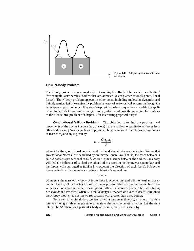
Another way to terminate is use three areas,A, B, andC, as shown in Figure 4.16. Thecomputation is terminated when the area computed for the largest of theA andB regions issufficiently close to the sum of the areas computed for the other two regions. For example,if regionB is the largest, terminate when the area ofB is sufficiently close to the area ofAplus the area ofC. Alternatively, we could simply terminate whenC is sufficiently small.Such methods are known asadaptive quadrature because the solution adapts to the shapeof the curve. (Simplified formulas can be derived for adaptive quadrature methods; seeFreeman and Phillips, 1992.)

Computations of areas under slowly varying parts of the curve stop earlier than com-putations of areas under more rapidly varying parts. The spacing,δ, will vary across theinterval. The consequence of this is that a fixed process assignment will not lead to the mostefficient use of processors. The load-balancing techniques described in Chapter 3, Section3.2.2, and in more detail in Chapter 7 are more appropriate. We should point out that somecare might be needed in choosing when to terminate. For example, the function such asshown in Figure 4.17 might cause us to terminate early, as two large regions are the same(i.e.,C = 0).

Figure 4.16 Adaptive quadratureconstruction.

A B

Cf(x)

x


4.2.3 N-Body Problem

TheN-body problem is concerned with determining the effects of forces between “bodies”(for example, astronomical bodies that are attracted to each other through gravitationalforces). TheN-body problem appears in other areas, including molecular dynamics andfluid dynamics. Let us examine the problem in terms of astronomical systems, although thetechniques apply to other applications. We provide the basic equations to enable the appli-cation to be coded as a programming exercise, which could use the same graphic routinesas the Mandelbrot problem of Chapter 3 for interesting graphical output.

Gravitational N-Body Problem. The objective is to find the positions andmovements of the bodies in space (say planets) that are subject to gravitational forces fromother bodies using Newtonian laws of physics. The gravitational force between two bodiesof massesma andmb is given by

whereG is the gravitational constant andr is the distance between the bodies. We see thatgravitational “forces” are described by an inverse square law. That is, the force between apair of bodies is proportional to 1/r 2, wherer is the distance between the bodies. Each bodywill feel the influence of each of the other bodies according to the inverse square law, andthe forces will sum together (taking into account the direction of each force). Subject toforces, a body will accelerate according to Newton’s second law:

F = ma

wherem is the mass of the body, F is the force it experiences, anda is the resultant accel-eration. Hence, all the bodies will move to new positions due to these forces and have newvelocities. For a precise numeric description, differential equations would be used (that is,F = mdv/dt andv = dx/dt, wherev is the velocity). However, an exact “closed” solution totheN-body problem is not known for systems with greater than three bodies.

For a computer simulation, we use values at particular times,t0, t1, t2 etc., the timeintervals being as short as possible to achieve the most accurate solution. Let the timeinterval be∆t. Then, for a particular body of massm, the force is given by

Figure 4.17 Adaptive quadrature with falsetermination.

f(x)

x

A B

C = 0

FGmamb

r2

------------------=


and a new velocity

wherevt+1 is the velocity of the body at timet + 1 andvt is the velocity of the body at timet. If a body is moving at a velocityv over the time interval∆t, its position changes by

wherext is its position at timet. Once bodies move to new positions, the forces change and

the computation has to be repeated.The velocity is not actually constant over the time interval, ∆t, and hence only an

approximate answer is obtained. It can help to use a “leap-frog” computation in whichvelocity and position are computed alternately; i.e.,

and

where the velocities are computed for timest, t + 1, t + 2, etc. and the positions arecomputed for timest + 1/2,t + 3/2,t + 5/2, etc.

Three-Dimensional Space. Since the bodies are in a three-dimensional space, allvalues are vectors and have to be resolved into three directions,x, y, andz. In a three-dimensional space having a coordinate system (x, y, z), the distance between the bodies at(xa, ya, za) and (xb, yb, zb) is given by

The forces are resolved in the three directions, using, for example,

where the particles are of massma and mb and have the coordinates (xa, ya, za) and(xb, yb, zb). Finally, the new position and velocity are computed. The velocity can also beresolved in three directions. For a simple computer solution, usually we assume a three-

Fm v

t 1+v

t–( )

∆t-------------------------------=

vt 1+

vt F∆t

m---------+=

xt 1+

xt

– v∆t=

Ft m v

t 1 2⁄+v

t 1 2⁄––( )

∆t--------------------------------------------------=

xt 1+

xt

– vt 1 2⁄+ ∆t=

r xb xa–( )2yb ya–( )2

zb za–( )2+ +=

Fx

Gmamb

r2

------------------xb xa–

r----------------

=

Fy

Gmamb

r2

------------------yb ya–

r----------------

=

Fz

Gmamb

r2

------------------zb za–

r---------------

=


dimensional space with fixed boundaries. Actually, the universe is continually expandingand does not have fixed boundaries!

Other Applications. Although we describe the problem in terms of astronomicalbodies, the concept can be applied to other situations. For example, charged particles arealso influenced by each other, in this case according to Coulomb’s electrostatic law (also aninverse square law of distance); particles of opposite charge are attracted and those of likecharge are repelled. A subtle difference between the problem and astronomical bodies isthat charged particles may move away from each other, whereas astronomical bodies areonly attracted and hence will tend to cluster.

Sequential Code. The overall gravitational N-body computation can bedescribed by the algorithm

for (t = 0; t < tmax; t++) /* for each time period */

for (i = 0; i < N; i++) { /* for each body */

F = Force_routine(i); /* compute force on i th body */

v[i] new = v[i] + F * dt; /* compute new velocity and

x[i] new = x[i] + v[i] new * dt; /* new position (leap-flog) */

}

for (i = 0; i < nmax; i++) { /* for each body */

x[i] = x[i] new; /* update velocity and position*/

v[i] = v[i] new;

}

Parallel Code. Parallelizing the sequential algorithm code can use simple parti-tioning whereby groups of bodies are the responsibility of each processor, and each forceis “carried” in distinct messages between processors. However, a large number of messagescould result. The algorithm is an O(N2) algorithm (for one iteration) as each of theN bodiesis influenced by each of the otherN − 1 bodies. It is not feasible to use this direct algorithmfor most interestingN-body problems whereN is very large.

The time complexity can be reduced using the observation that a cluster of distantbodies can be approximated as a single distant body of the total mass of the cluster sited atthe center of mass of the cluster, as illustrated in Figure 4.18. This clustering idea can beapplied recursively.

Distant cluster of bodiesr

Center of mass

Figure 4.18 Clustering distant bodies.


Barnes-Hut Algorithm. A clever divide-and-conquer formation to the problemusing this clustering idea starts with the whole space in which one cube contains the bodies(or particles). First, this cube is divided into eight subcubes. If a subcube contains no par-ticles, the subcube is deleted from further consideration. If a subcube contains more thanone body, it is recursively divided until every subcube contains one body. This processcreates anocttree; that is, a tree with up to eight edges from each node. The leaves representcells each containing one body. (We assumed the original space is a cube so that cubesresult at each level of recursion, but other assumptions are possible.)

For a two-dimensional problem, each recursive subdivision will create four subareasand aquadtree (a tree with up to four edges from each edge; see Section 4.1.3). In general,the tree will be very unbalanced. Figure 4.19 illustrates the decomposition for a two-dimen-sional space (which is easier to draw) and the resultant quadtree. The three-dimensionalcase follows the same construction except with up to eight edges from each node.

In the Barnes-Hut algorithm (Barnes and Hut, 1986), after the tree has been con-structed, the total mass and center of mass of the subcube is stored at each node. The forceon each body can then be obtained by traversing the tree starting at the root, stopping at anode when the clustering approximation can be used for the particular body, and otherwisecontinuing to traverse the tree downward. In astronomicalN-body simulations, a simplecriterion for when the approximation can be made is as follows. Suppose the cluster isenclosed in a cubic volume given by the dimensionsd × d × d, and the distant to the centerof mass isr. Use the clustering approximation when

whereθ is a constant typically 1.0 or less (θ is called the opening angle). This approach cansubstantially reduce the computational effort.

Subdivisiondirection

Figure 4.19 Recursive division of two-dimensional space.

Partial quadtreeParticles

rdθ---≥


Once all the bodies have been given new positions and velocities, the process isrepeated for each time period. This means that the whole octtree must be reconstructed foreach time period (because the bodies have moved). Constructing the tree requires a time ofΟ(nlogn), and so does computing all the forces, so that the overall time complexity of themethod is O(nlogn) (Barnes and Hut, 1986).

The algorithm can be described by the following:

for (t = 0; t < tmax; t++) { /* for each time period */

Build_Octtree(); /* construct Octtree (or Quadtree) */

Tot_Mass_Center(); /* compute total mass & center /*

Comp_Force(); /* traverse tree/computing forces */

Update(); /* update position/velocity */

}

The Build_Octtree() routine can be constructed from the positions of the bodies,considering each body in turn. TheTot_Mass_Center() routine must traverse the tree,computing the total mass and center of mass at each node. This could be done recursively.The total mass,M, is given by the simply sum of the total masses of the children:

wheremi is the total mass of theith child. The center of mass,C, is given by

where position of the centers of mass have three components, in thex, y, andz directions.TheComp_Force() routine must visit nodes ascertaining whether the clustering approxima-tion can be applied to compute the force of all the bodies in that cell. If the clusteringapproximation cannot be applied, the children of the node must be visited.

The octtree will, in general, be very unbalanced, and its shape changes during thesimulation. Hence, a simple static partitioning strategy will not be very effective in load bal-ancing. A better way of dividing the bodies into groups is calledorthogonal recursivebisection (Salmon, 1990). Let us describe this method in terms of a two-dimensional squarearea. First, a vertical line is found that divides the area into two areas each with an equalnumber of bodies. For each area, a horizontal line is found that divides it into two areas eachwith an equal number of bodies. This is repeated until there are as many areas as processors,and then one processor is assigned to each area. An example of the division is illustrated inFigure 4.20.

M mi

i 0=

7

∑=

C1M----- mi ci×( )

i 0=

7

∑=

Chap. 4 Further Reading 131

4.3 SUMMARY

This chapter introduced the following concepts:

• Partitioning and divide-and-conquer concepts as the basis for parallel computingtechniques

• Tree constructions

• Examples of partitioning and divide-and-conquer problems — namely, bucket sort,numerical integration, and theN-body problem

F U R T H E R R E A D I N G

The divide-and-conquer technique is described in many sequential programming texts (forexample, Kruse, 1994). As we have seen, this technique results in a tree structure. It ispossible to construct a multiprocessor with a tree network, which would then be amenableto divide-and-conquer problems. One or two tree network machines have been constructedwith the thought that most applications can be formulated as divide and conquer. However,as we have seen in Chapter 1, trees can be embedded into meshes and hypercubes so that itis not necessary to have tree network. Mapping divide-and-conquer algorithms ontodifferent architectures is the subject of research papers, such as that done by Lo andRajopadhye (1990).

Once a problem is partitioned, in some contexts a scheduling algorithm is appropriatefor allocating processors to partitions or processes. Several texts explore scheduling,including Quinn (1994), Lewis and El-Rewini (1992), Moldovan (1993), and Sarkar(1989). Mapping (static scheduling) is not considered in this text. However, dynamic loadbalancing, in which tasks are assigned to processors during the execution of the program,is considered in Chapter 7.

Bucket sort is described in texts on sorting algorithms (see Chapter 9) and can befound specifically in Lindstrom (1985) and Wagner and Han (1986). Numerical evaluationof integrals in the context of parallel programs can be found in Freeman and Phillips (1992),

Figure 4.20 Orthogonal recursive bisectionmethod.


Gropp, Lusk, and Skjellum (1994), Lester (1993), and Smith (1993) and is often used as asimple application of parallel programs. The original source for the Barnes-Hut algorithmis Barnes and Hut (1986). Other papers include Bhatt et al. (1992) and Warren and Salmon(1992). Liu and Wu (1997) consider programming the algorithm inn C++. Apart from theBarnes-Hutt divide-and-conquer algorithm, another approach is the fast multipole method(Greengard and Rokhlin, 1987). Hybrid methods exist.

B I B L I O G R A P H Y

AHO, A. V., J. E. HOPCROFT, AND J. D. ULLMAN (1974),The Design and Analysis of ComputerAlgorithms, Addison-Wesley, Reading, Massachusetts.

BARNES, J. E.,AND P. HUT (1986), “A Hierarchical O(NlogN) Force Calculation Algorithm,” Nature,Vol. 324, No. 4 (December), pp. 446–449.

BHATT, S., M. CHEN, C. Y. LIN, AND P. LIU (1992), “Abstractions for ParallelN-Body Simulations,”Proc. Scalable High Performance Computing Conference, pp. 26–29.

BLELLOCH, G. E. (1996), “Programming Parallel Algorithms,”Comm. ACM, Vol. 39, No. 3, pp. 85–97.

BOKHARI, S. H. (1981), “On the Mapping Problem,” IEEE Trans. Comput., Vol. C-30, No. 3, pp. 207–214.

FREEMAN, T. L., AND C. PHILLIPS (1992),Parallel Numerical Algorithms, Prentice Hall, London.

GREENGARD, L., AND V. ROKHLIN (1987), “A Fast Algorithm for Particle Simulations,” J. Comp.Phys., Vol. 73, pp. 325–348.

GROPP, W., E. LUSK, AND A. SKJELLUM (1994),Using MPI Portable Parallel Programming with theMessage-Passing Interface, MIT Press, Cambridge, Massachusetts.

JÁJÁ, J. (1992), An Introduction to Parallel Algorithms, Addison Wesley, Reading, Massachusetts.

KRUSE, R. L. (1994), Data Structures and Program Design, 3rd ed., Prentice Hall, Englewood Cliffs,New Jersey.

KUMAR, V., A. GRAMA, A. GUPTA, AND G. KARYPIS (1994),Introduction to Parallel Computing,Benjamin/Cummings, Redwood City, California.

LESTER, B. (1993),The Art of Parallel Programming, Prentice Hall, Englewood Cliffs, New Jersey.

LEWIS, T. G., AND H. EL-REWINI (1992), Introduction to Parallel Computing, Prentice Hall,Englewood Cliffs, New Jersey.

LINDSTROM, E. E. (1985), “The Design and Analysis of BucketSort for Bubble Memory SecondaryStorage,”IEEE Trans. Comput., Vol. C-34, No. 3, pp. 218–233.

LIU, P.,AND J.-J. WU (1997), “A Framework for Parallel Tree-Based Scientific Simulations,” Proc.1997 Int. Conf. Par. Proc., pp. 137–144.

LO, V. M., AND S. RAJOPADHYE (1990), “Mapping Divide-and-Conquer Algorithms to ParallelArchitectures,”Proc. 1990 Int. Conf. Par. Proc., Part III, pp. 128–135.

MILLER, R., AND Q. F. STOUT (1996),Parallel Algorithms for Regular Architectures: Meshes andPyramids, MIT Press, Cambridge, Massachusetts.

MOLDOVAN, D. I. (1993),Parallel Processing from Applications to Systems, Morgan Kaufmann, SanMateo, California.

PREPARATA, F. P.,AND M. I. SHAMOS (1985),Computational Geometry: An Introduction, Springer-Verlag, New York.

Chap. 4 Problems 133

QUINN, M. J. (1994),Parallel Computing Theory and Practice, McGraw-Hill, New York.

SALMON, J. K. (1990),Parallel Hierarchical N-Body Methods, Ph.D. thesis, California Institute ofTechnology.

SARKAR, V. (1989),Partitioning and Scheduling Parallel Programs for Multiprocessing, MIT Press,Cambridge, Massachusetts.

SMITH, J. R. (1993),The Design and Analysis of Parallel Algorithms, Oxford UP, Oxford.

WAGNER, R. A., AND Y. HAN (1986), “Parallel Algorithms for Bucket Sorting and Data DependentPrefix Problem,”Proc. 1986 Int. Conf. Par. Proc., pp. 924–929.

WARREN, M., AND J. SALMON (1992), “AstrophysicalN-Body Simulations Using Hierarchical TreeData Structures,”Proc. Supercomputing 92, IEEE CS Press, Los Alamitos, pp. 570–576.

P R O B L E M S

Scientific/Numerical

4-1. Write a program that will prove that the maximum speedup of adding a series of numbers usinga simple partition described in Section 4.1.1 ism/2, where there arem processes.

4-2. Using the equations developed in Section 4.1.1 for partitioning a list of numbers intom parti-tions that are added separately, show that the optimum value form to give the minimum parallelexecution time is when , where there arep processors. (Clue: Differen-tiate the parallel execution time equation.)

4-3. Section 4.1.1 gives three implementations of adding numbers, using separatesend() s andrecv() s, using a broadcast routine with separaterecv() s to return partial results and usingscatter and reduce routines. Write parallel programs for all three implementations, instrument-ing the programs to extract timing information (Chapter 2, Section 2.3.4), and compare theresults.

4-4. Suppose the structure of a computation consists of a binary tree withn leaves (final tasks) andlogn levels. Each node in the tree consists of one computational step. What is the lower boundof the execution time if the number of processors is less thann?

4-5. Analyze the divide-and-conquer method of assigning one processor to each node in a tree foradding numbers (Section 4.1.2) in terms of communication, computation, overall parallelexecution time, speedup, and efficiency.

4-6. Complete the parallel pseudocode given in Section 4.1.2 for the (binary) divide-and-conquermethod for all eight processes.

4-7. Develop the equations for computation and communication times form-ary divide andconquer, following the approach used in Section 4.1.2.

4-8. Develop a divide-and-conquer algorithm that finds the smallest value in a set ofn values inΟ(logn) steps usingn/2 processors. What is the time complexity if there are fewer thann/2 pro-cessors?

4-9. Write a parallel program with a time complexity ofΟ(logn) to compute the polynomial

f = a0x0 + a1x1 + a2x

2 + … +an−1xn−1

to any degree,n, where thea’s, x, andn are input.

4-10. Write a parallel program that uses a divide-and-conquer approach to find the first zero in a listof integers stored in an array. Use 16 processes and 256 numbers.

m p 1 tstartup+( )⁄=


4-11. Write parallel programs to compute the summation ofn integers in each of the following waysand assess their performance. Assume thatn is a power of 2.(a) Partition then integers inton/2 pairs. Usen/2 processes to add together each pair of

integers resulting inn/2 integers. Repeat the method on then/2 integers to obtainn/4integers and continue until the final result is obtained. (This is a binary tree algorithm.)

(b) Divide then integers inton/logn groups of logn numbers each. Usen/logn processes,each adding the numbers in one group sequentially. Then add then/logn results usingmethod (a). This algorithm is shown in Figure 4.21.

4-12. Write parallel programs to computen! in each of the following ways and assess their perfor-mance. The number,n, may be odd or even but is a positive constant.(a) Computen! using two concurrent processes, each computing approximately half of the

complete sequence. A master process then combines the two partial results.

(b) Computen! using a producer process and a consumer process connected together. Theproducer produces the numbers 1, 2, 3, …n in sequence. The consumer accepts thesequence of numbers from the producer and accumulates the result; i.e., 1× 2 × 3 … .

4-13. Write a divide-and-conquer parallel program that determines whether the number of 1’s in abinary file is even or odd (i.e., create a parity checker). Modify the program so that a bit isattached to the contents of the file, and set to a 0 or a 1 to make the number of 1’s even (a paritygenerator).

4-14. One way to computeπ is to compute the area under the curvef(x) = 4/(1+ x2) between 0 and1, which is numerically equal toπ. Write a parallel program to calculateπ this way using 10processes. Another way to computeπ is to compute the area of a circle of radiusr = 1 (i.e.,πr 2 = π). Determine the appropriate equation for a circle, and write a parallel program tocomputeπ this way. Comment on the two ways of computingπ.

+

+

+

+

+

+

+

+

+

+

+

+

+

+

+

Binary Tree

Result

Figure 4.21 Process diagram for Problem 4-12(b).

logn numbers


4-15. Derive a formula to evaluate numerically an integral using the adaptive quadrature methoddescribed in Section 4.2.2. Use the approach given for the trapezoidal method.

4-16. Using any method, write a parallel program that will compute the integral

4-17. Write a static assignment parallel program to computeπ using the formula

using each of the following ways:

1. Rectangular decomposition, as illustrated in Figure 4.13

2. Rectangular decomposition, as illustrated in Figure 4.14

3. Trapezoidal decomposition, as illustrated in Figure 4.15

Evaluate each method in terms of speed and accuracy.

4-18. Find the zero crossing of a function by a bisection method. In this method, two points on thefunction are computed, sayf(a) and f(b), where f(a) is positive andf(b) is negative. Thefunction must cross somewhere betweenf(a) and f(b), as illustrated in Figure 4.22. By

successively dividing the interval, the exact location of the zero crossing can be found. Writea divide-and-conquer program that will find the zero crossing locations of the functionf(x) = x2 − 3x + 2. (This function has two zero crossing locations,x = 1 andx = 2.)

4-19. Write a parallel program to integrate a function using Simpson’s rule, which is given asfollows:

whereδ is fixed [δ = (b − a)/n andn must be even]. Choose a suitable function (or arrange itso that the function can be input).

4-20. Write a sequential program and a parallel program to simulate an astronomicalN-body system,but in two-dimensions. The bodies are initially at rest. Their initial positions and masses are tobe selected randomly (using a random number generator). Display the movement of the bodiesusing the graphical routines used for the Mandelbrot program found in http://

I x1x---

sin+ xd

0.01

1∫=

1 x2– xd0

1∫ π4---=

f(a)

f(b)

ab

y

x

f(x)

Figure 4.22 Bisection method for findingthe zero crossing location of a function.

I f x( ) xda

b∫= =

δ3--- f a( ) 4 f a δ+( ) 2 f a 2δ+( ) 4 f a 3δ+( ) 2 f a 4δ+( ) …4 f a n 1–( )δ+( ) f b( )+ + + + + +[ ]


www.cs.uncc.edu/par_prog, or otherwise, showing each body in a color and size to indicate itsmass.

4-21. Develop theN-body equations for a system of charged particles (e.g., free electrons andpositrons) that are governed by Coulumb’s law. Write a sequential and a parallel program tomodel this system, assuming that the particles lie in a two-dimensional space. Producegraphical output showing the movement of the particles. Provide your own initial distributionand movement of particles and solution space.

4-22. (Research problem) Given a set ofn points in a plane, develop an algorithm and parallelprogram to find the points that are on the perimeter of the smallest region containing all of thepoints, and join the points, as illustrated in Figure 4.23. This problem is known as the planarconvex hull problem and can be solved by a recursive divide-and-conquer approach verysimilar to quicksort, by recursively splitting regions into two parts using “pivot” points. Thereare several sources for information on the planar convex hull problem, including Blelloch(1996), Preparata and Shamos (1985), and Miller and Stout (1996).

Real Life

4-23. Write a sequential and a parallel program to model the planets around the sun (or another as-tronomical system). Produce graphical output showing the movement of the planets. Provideyour own initial distribution and movement of planets. (Use real data if available.)

4-24. A major bank in your state processes an average of 30million checks a day for its 2millioncustomer accounts. One time-consuming problem is that of sorting the checks into individualcustomer-account bundles so they can be returned with the monthly statements. (Yes, the bankhandles check sorting for several client banks in addition to its own.) The bank has been usinga very fast mainframe-based check sorter and the quicksort method. However, you have toldthe bank that you know of a way to useN smaller computers in parallel, with each sorting1/Nth of the 30million checks, and then merge those partial sorts into a single sorted result.Prior to the bank actually investing in the new technology, you have been hired as a consultantto simulate the process using message-passing parallel programming. Under the followingassumptions, simulate this new approach for the bank.

Assumptions:

1. Each check has three identification numbers: a nine-digit bank-identification number, anine-digit account-identification number, and a three-digit check number (leading zerosare not printed or shown).

2. All checks with the same bank-identification number are to be sorted by customeraccount for transmittal to that client bank.

Figure 4.23 Convex hull (Problem 4-22).


Estimate the speedup ifN is 10; ifN is 1000. Estimate the percentage of time spent in commu-nications versus time spent in processing.

4-25. Sue, 21 years old, comes from a very financially astute family. She has been watching herparents save and invest for several years now, reads theWall Street Journal daily in the univer-sity library (for free!), and has concluded that she will not be able to rely on social securitywhen she retires in 49 years. For graduation from college, her parents got her a CD-ROM con-taining historical daily closing prices covering every exchange-listed security, from January 1,1900 to the end of last month.

For simplicity you may think of the data on the CD-ROM as being organized into date/symbol/closing price records for each of the 358,000 securities that have been listed since1900. (Only a fraction are listed at any given date; firms go out of business and new ones startdaily.) Similarly, you may assume that the format of a record is given by

date Last three digits of the year, followed by the “Julian date” (where January 15is Julian 15, February 1 is Julian 32, etc.)

symbol Up to 10 characters, such as PCAI, KAUFX, or IBM.AZ, representing aNASDAQ stock (PCA International), a mutual fund (Kaufman AggressiveGrowth), and an option to buy IBM stock at a particular price for a particularlength of time, respectively.

closing price Three integers, X (representing a whole number of dollars per unit),Y(representing the numerator of a fractional dollar per unit), andZ(representing the denominator of a fractional dollar per unit).

For example, “996033/PCAI/10/3/4” indicates that on February 2, 1996, PCA Internationalstock closed at $10.75 per share. Sue wants to know how many of the stocks that were listedas of last month’s end have had 50 or more consecutive trading days in which they closed eitherunchanged from the previous day or closed at a higher price, anytime in the CD-ROM’s“recorded history.”

4-26. The more Samantha recalled her grandfather’s stories about the time he won the 1963 WorldChampionship Dominos Match, the more she wanted to improve her skills at the game. Shehad a basic problem though; she had no playing partners left, having already improved to thepoint where she consistently won every game against the few friends who still remained!

Samantha knew that computerized versions of Go, chess, bridge, poker, and checkershad been developed, and saw no reason someone skilled in the science of computers could notdo the same for dominos. One of her computer science professors at the new campus of theUniversity of Canada, U-Can-II, had told her she could do anything she wanted (within theo-retical limitations, of course), and shereally wanted to win that next World Championship!

Pulling out her slow, old, nearly obsolete 300MHz/64 Meg (RAM)/6 Gbyte (disk)Pentium, she quickly developed a straightforward, single processor simulator that she couldpractice against. The basic outline of her approach was to have the program compare every oneof its pieces to the pieces already played in order to determine the computer’s best move. Thisappeared to involve enough computation, including rotations and trial placements of pieces,that Samantha found herself waiting for the program to produce the computer’s next move, andbecoming as bored with its game performance as with that of her old friends. Thus, she isseeking your assistance in developing a parallel processor version.

1. Outline her single processor algorithm.2. Outline your parallel processor algorithm.3. Estimate the speedup that could be obtained if you were to network 50 old computers

like hers, and make a recommendation to her about either going ahead with the task orspending $2500 to buy the new 800MHz “Octium,” which is reputed to be 50 timesfaster than her old Pentium for these kinds of simulations.


4-27. Area, Inc., provides a numerical integration service for several small engineering firms in theregion. When any of those firms has a continuous function defined over a domain and is unableto integrate it, Area, Inc., gets the call. You have just been hired to help Area, Inc., improve itsslow delivery of computed integration results. Area, Inc. has lost money each year of itsexistence and is so “nonprofit” that payment of next week’s payroll is in question. Given yourdesire to continue eating (and for that to continue, Area, Inc., has to pay you), you have con-siderable incentive to help Area, Inc.

Given also that you have a considerable background in parallel computing, yourecognize the problem immediately: Area, Inc., has been using a single processor to implementa standard numerical integration algorithm.

Step 1: Divide the independent axis intoN even intervals.

Step 2: Approximate the area under the function in any interval (its integral over that interval),by the product of the interval width times the function value when it is evaluated at theleft edge of the interval.

Step 3: Add up allN approximations to get the total area.

Step 4: Divide the interval width in half.

Step 5: Repeat steps 1– 4 until the total from theith repetition differs from the (i − 1)threpetition by less than 0.001% of the magnitude of theith total.

Since your manager is skeptical about new-fangled parallel computing approaches, she wantsyou to simulate two different machine configurations: two processors in the first, and eight pro-cessors in the second. She has told you that a successful demonstration is key to being able tobuy more processors and to your getting paid next week.

Partitioning and Divide-and-Conquer Strategies · 108 Partitioning and Divide-and-Conquer...

Documents

Transcript of Partitioning and Divide-and-Conquer Strategies · 108 Partitioning and Divide-and-Conquer...