Parties, Models, Mobsters - uibk.ac.atzeileis/papers/NUS-2014.pdf · Parties, Models, Mobsters A...

Parties, Models, MobstersA New Implementation of Model-Based Recursive Partitioning in R

Achim Zeileis, Torsten Hothorn

http://eeecon.uibk.ac.at/~zeileis/

http://eeecon.uibk.ac.at/~zeileis/

Overview

Motivation: Trees and leavesModel-based (MOB) recursive partitioning

Model estimationTests for parameter instabilitySegmentationPruningLocal models

Implementation in RBuilding blocks: Parties, models, mobstersOld implementation in partyAll new implementation in partykit

ApplicationPaired comparisons for Germany’s Topmodel finalistsBradley-Terry treesImplementation from scratch

Motivation: Trees

Breiman (2001, Statistical Science) distinguishes two cultures ofstatistical modeling.

Data models: Stochastic models, typically parametric.→ Classical strategy in statistics. Regression models are still theworkhorse for many empirical analyses.

Algorithmic models: Flexible models, data-generating processunknown. → Still few applications in many fields, e.g., socialsciences or economics.

Classical example: Trees, i.e., modeling of dependent variable y by“learning” a recursive partition w.r.t explanatory variables z1, . . . , zl .

Motivation: Leaves

Key features:1 Predictive power in nonlinear regression relationships.2 Interpretability (enhanced by visualization), i.e., no “black box”

methods.

Typically: Simple models for univeriate y , e.g., mean.

Idea: More complex models for more complex y , e.g., regressionmodels, multivariate normal model, item responses, etc.

Here: Synthesis of parametric data models and algorithmic treemodels.

Goal: Fitting local models by partitioning of the sample space.

Recursive partitioning

Model-based (MOB) algorithm:

1 Fit the parametric model in the current subsample.2 Assess the stability of the parameters across each partitioning

variable zj .3 Split sample along the zj∗ with strongest instability: Choose

breakpoint with highest improvement of the model fit.4 Repeat steps 1–3 recursively in the subsamples until some

stopping criterion is met.


Example: Logistic regression, assessing differences in the effect of“preferential treatment” (“women and children first”?) in the Titanicsurvival data.

In R: Generalized linear model tree with binomial family (and defaultlogit link).

R> mb <- glmtree(Survived ~ Treatment | Age + Gender + Class,+ data = ttnc, family = binomial, alpha = 0.05, prune = "BIC")R> plot(mb)R> print(mb)

Result: Log-odds ratio of survival given treatment differs acrossclasses (slope), as does the survival probability of male adults(intercept).


Classp < 0.001

1

3rd 1st, 2nd, Crew

Node 2 (n = 706)

Normal(Male&Adult)

Preferential(Female|Child)

Yes

No

0

0.2

0.4

0.6

0.8

1

●

●

Classp < 0.001

3

2nd 1st, Crew

Node 4 (n = 285)

Normal(Male&Adult)


Yes

No

0

0.2

0.4

0.6

0.8

1

●

●

Node 5 (n = 1210)

Normal(Male&Adult)


Yes

No

0

0.2

0.4

0.6

0.8

1

●

●


Generalized linear model tree (family: binomial)

Model formula:Survived ~ Treatment | Age + Gender + Class

Fitted party:[1] root| [2] Class in 3rd: n = 706| (Intercept) TreatmentPreferential| -1.641 1.327| [3] Class in 1st, 2nd, Crew| | [4] Class in 2nd: n = 285| | (Intercept) TreatmentPreferential| | -2.398 4.477| | [5] Class in 1st, Crew: n = 1210| | (Intercept) TreatmentPreferential| | -1.152 4.318

Number of inner nodes: 2Number of terminal nodes: 3Number of parameters per node: 2Objective function (negative log-likelihood): 1061

1. Model estimation

Models: M(y , x , θ) with (potentially multivariate) observations y ,optionally regressors x , and k -dimensional parameter vector θ ∈ Θ.

Parameter estimation: θ̂ by optimization of additive objective functionΨ(y , x , θ) for n observations yi (i = 1, . . . , n):

θ̂ = argminθ∈Θ

n∑i=1

Ψ(yi , xi , θ).

Special cases: Maximum likelihood (ML), weighted and ordinary leastsquares (OLS and WLS), quasi-ML, and other M-estimators.

1. Model estimation

Estimating function: θ̂ can also be defined in terms of

n∑i=1

ψ(yi , xi , θ̂) = 0,

where ψ(y , x , θ) = ∂Ψ(y , x , θ)/∂θ.

Central limit theorem: If there is a true parameter θ0 and given certainweak regularity conditions:

√n(θ̂ − θ0)

d−→ N (0,V (θ0)),

where V (θ0) = {A(θ0)}−1B(θ0){A(θ0)}−1. A and B are theexpectation of the derivative of ψ and the variance of ψ, respectively.

1. Model estimation

Idea: In many situations, a single global modelM(y , x , θ) that fits alln observations cannot be found. But it might be possible to find apartition w.r.t. the variables z1, . . . , zl so that a well-fitting model can befound locally in each cell of the partition.

Tools:

Assess parameter instability w.r.t to partitioning variableszj (j = 1, . . . , l).

A general measure of deviation from the model is the estimatingfunction ψ(y , x , θ).

2. Tests for parameter instability

Generalized M-fluctuation tests capture instabilities in θ̂ for an orderingw.r.t zj .

Basis: Empirical fluctuation process of cumulative deviations w.r.t. toan ordering σ(zij).

Wj(t, θ̂) = B̂−1/2n−1/2bntc∑i=1

ψ(yσ(zij ), xσ(zij ), θ̂) (0 ≤ t ≤ 1)

Functional central limit theorem: Under parameter stabilityWj(·)

d−→ W 0(·), where W 0 is a k -dimensional Brownian bridge.


zj

y

2004 2006 2008 2010 2012

200

400

600

800

1000

1200

zj

Flu

ctua

tion

Pro

cess

2004 2006 2008 2010 2012

−4

−2

02

4


Test statistics: Scalar functional λ(Wj) that captures deviations fromzero.

Null distribution: Asymptotic distribution of λ(W 0).

Special cases: Class of test encompasses many well-known tests fordifferent classes of models. Certain functionals λ are particularlyintuitive for numeric and categorical zj , respectively.

Advantage: ModelM(y , x , θ̂) just has to be estimated once. Empiricalestimating functions ψ(yi , xi , θ̂) just have to be re-ordered andaggregated for each zj .


Splitting numeric variables: Assess instability using supLM statistics.

λsupLM(Wj) = maxi=ı̇,...,ı

(in· n − i

n

)−1 ∣∣∣∣∣∣∣∣Wj

(in

)∣∣∣∣∣∣∣∣22.

Interpretation: Maximization of single shift LM statistics for allconceivable breakpoints in [ı̇, ı].

Limiting distribution: Supremum of a squared, k -dimensionaltied-down Bessel process.

Potential alternatives: Many other parameter instability tests from thesame class of tests, e.g., a Cramér-von Mises test (or Nyblom-Hansentest), MOSUM tests, etc.


Splitting categorical variables: Assess instability using χ2 statistics.

λχ2(Wj) =C∑

c=1

n|Ic|

∣∣∣∣∣∣∣∣∆Ic Wj

(in

)∣∣∣∣∣∣∣∣22.

Feature: Invariant for re-ordering of the C categories and theobservations within each category.

Interpretation: Capture instability for split-up into C categories.

Limiting distribution: χ2 with k · (C − 1) degrees of freedom.


Splitting ordinal variables: Several strategies conceivable. Assessinstability either as for categorical variables (if C is low), or as fornumeric variables (if C is high), or via a specialized test.

λmaxLMo(Wj) = maxi∈{i1,...,iC−1}

(in· n − i

n

)−1 ∣∣∣∣∣∣∣∣Wj

(in

)∣∣∣∣∣∣∣∣22,

λWDMo(Wj) = maxi∈{i1,...,iC−1}

(in· n − i

n

)−1/2 ∣∣∣∣∣∣∣∣Wj

(in

)∣∣∣∣∣∣∣∣∞.

Interpretation: Assess only the possible splitpoints i1, . . . , iC−1, basedon L2 or L∞ norm.

Limiting distribution: Maximum from selected points in a squaredBessel process or multivariate normal distribution, respectively.

3. Segmentation

Goal: Split model into b = 1, . . . ,B segments along the partitioningvariable zj associated with the highest parameter instability. Localoptimization of ∑

b

∑i∈Ib

Ψ(yi , xi , θb).

B = 2: Exhaustive search of order O(n).

B > 2: Exhaustive search is of order O(nB−1), but can be replaced bydynamic programming of order O(n2). Different methods (e.g.,information criteria) can choose B adaptively.

Here: Binary partitioning. Optionally, B = C can be chosen (withoutsearch) for categorical variables.

4. Pruning

Goal: Avoid overfitting.

Pre-pruning:

Internal stopping criterium.

Stop splitting when there is no significant parameter instability.

Based on Bonferroni-corrected p values of the fluctuation tests.

Post-pruning:

Grow large tree (e.g., with high significance level).

Prune splits that do not improve the model fit based on informationcriteria (e.g., AIC or BIC).

Hyperparameters: Significance level and information criterion penaltycan be chosen manually (or possibly through cross-validation etc.).

Local models

Goals:

Detection of interactions and nonlinearities in regressions.

Add explanatory variables for models without regressors.

Detect violations of parameter stability (measurement invariance)across several variables adaptively.

Mobsters:

Linear and generalized linear model trees (Zeileis et al. 2008).

Censored survival regression trees: parametric proportionalhazard and accelerated failure time models (Zeileis et al. 2008).

Beta regression trees (Grün et al. 2012).

Bradley-Terry trees for paired comparisons (Strobl et al. 2011).

Item response theory (IRT) trees: Rasch, rating scale and partialcredit model (Strobl et al. 2014, Abou El-Komboz et al. 2014).

Implementation: Building blocks

Workhorse function: mob() for

data handling,

calling model fitters,

carrying out parameter instability tests and

recursive partitioning algorithm.

Required functionality:

Parties: Class and methods for recursive partytions.

Models: Fitting functions for statistical models (optimizing suitableobjective function).

Mobsters: High-level interfaces (lmtree(), bttree(), . . . ) thatcall lower-level mob() with suitable options and methods.

Implementation: Old mob() in party

Parties: S4 class ‘BinaryTree’.

Originally developed only for ctree() and somewhat “abused”.

Rather rigid and hard to extend.

Models: S4 ‘StatModel’ objects.

Intended to conceptualize unfitted model objects.

Required some “glue code” to accomodate non-standard interfacefor data handling and model fitting.

Mobsters:

mob() already geared towards (generalized) linear models.

Other interfaces in psychotree and betareg.

Hard to do fine control due to adopted S4 classes: Manyunnecessary computations and copies of data.

Implementation: New mob() in partykit

Parties: S3 class ‘modelparty’ built on ‘party’.

Separates data and tree structure.

Inherits generic infrastructure for printing, predicting, plotting, . . .

Models: Plain functions with input/output convention.

Basic and extended interface for rapid prototyping and forspeeding up computings, respectively.

Only minimial glue code required if models are well-designed.

Mobsters:

mob() completely agnostic regarding models employed.

Separate interfaces lmtree(), glmtree(), . . .

New interfaces typically need to bring their model fitter and adaptthe main methods print(), plot(), predict() etc.

Implementation: New mob() in partykit

New inference options: Not used by default by optionally available.

New parameter instability tests for ordinal partitioning variables.Alternative to unordered χ2 test but computationally intensive.

Post-pruning based on information criteria (e.g., AIC or BIC),especially for very large datasets where traditional significancelevels are not useful.

Multiway splits for categorical partitioning variables.

Treat weights as proportionality weights and not as case weights.

Implementation: Models

Input: Basic interface.

fit(y, x = NULL, start = NULL, weights = NULL,

offset = NULL, ...)

y, x, weights, offset are (the subset of) the preprocessed data.Starting values and further fitting arguments are in start and ....

Output: Fitted model object of class with suitable methods.

coef(): Estimated parameters θ̂.

logLik(): Maximized log-likelihood function −∑

i Ψ(yi , xi , θ̂).

estfun(): Empirical estimating functions Ψ′(yi , xi , θ̂).

Implementation: Models

Input: Extended interface.

fit(y, x = NULL, start = NULL, weights = NULL,

offset = NULL, ..., estfun = FALSE, object = FALSE)

Output: List.

coefficients: Estimated parameters θ̂.

objfun: Minimized objective function∑

i Ψ(yi , xi , θ̂).

estfun: Empirical estimating functions Ψ′(yi , xi , θ̂). Only neededif estfun = TRUE, otherwise optionally NULL.

object: A model object for which further methods could beavailable (e.g., predict(), or fitted(), etc.). Only needed ifobject = TRUE, otherwise optionally NULL.

Internally: Extended interface constructed from basic interface ifsupplied. Efficiency can be gained through extended approach.

Implementation: Parties

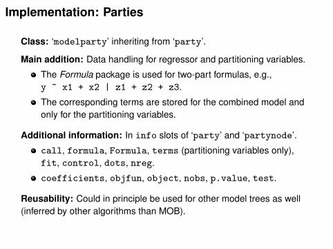
Class: ‘modelparty’ inheriting from ‘party’.

Main addition: Data handling for regressor and partitioning variables.

The Formula package is used for two-part formulas, e.g.,y ~ x1 + x2 | z1 + z2 + z3.

The corresponding terms are stored for the combined model andonly for the partitioning variables.

Additional information: In info slots of ‘party’ and ‘partynode’.

call, formula, Formula, terms (partitioning variables only),fit, control, dots, nreg.

coefficients, objfun, object, nobs, p.value, test.

Reusability: Could in principle be used for other model trees as well(inferred by other algorithms than MOB).

Bradley-Terry trees

Questions: Which of thesewomen is more attractive?How does the answer depend onage, gender, and the familiaritywith the associated TV showGermany’s Next Topmodel?

Bradley-Terry trees

Task: Preference scaling of attractiveness.

Data: Paired comparisons of attractiveness.

Germany’s Next Topmodel 2007 finalists: Barbara, Anni, Hana,Fiona, Mandy, Anja.

Survey with 192 respondents at Universität Tübingen.

Available covariates: Gender, age, familiarty with the TV show.

Familiarity assessed by yes/no questions: (1) Do you recognize thewomen?/Do you know the show? (2) Did you watch it regularly?(3) Did you watch the final show?/Do you know who won?

Bradley-Terry trees

Model: Bradley-Terry (or Bradley-Terry-Luce) model.

Standard model for paired comparisons in social sciences.

Parametrizes probability πij for preferring object i over j in terms ofcorresponding “ability” or “worth” parameters θi .

πij =θi

θi + θj

logit(πij) = log(θi)− log(θj)

Maximum likelihood as a logistic or log-linear GLM.

Mobster: bttree() in psychotree (Strobl et al. 2011).

Here: Use mob() directly to build model from scratch usingbtReg.fit() from psychotools.

Bradley-Terry trees

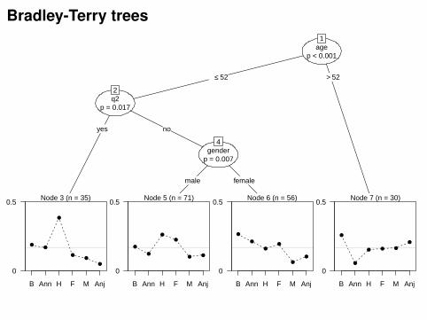
agep < 0.001

1

≤ 52 > 52

q2p = 0.017

2

yes no

Node 3 (n = 35)

●●

●

●●

●

B Ann H F M Anj

0

0.5

genderp = 0.007

4

male female

Node 5 (n = 71)

●

●

●

●

● ●

B Ann H F M Anj

0

0.5Node 6 (n = 56)

●

●

●

●

●

●

B Ann H F M Anj

0

0.5Node 7 (n = 30)

●

●

● ● ●

●

B Ann H F M Anj

0

0.5

Bradley-Terry trees

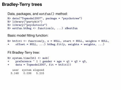
Data, packages, and estfun() method:R> data("Topmodel2007", package = "psychotree")R> library("partykit")R> library("psychotools")R> estfun.btReg <- function(x, ...) x$estfun

Basic model fitting function:

R> btfit1 <- function(y, x = NULL, start = NULL, weights = NULL,+ offset = NULL, ...) btReg.fit(y, weights = weights, ...)

Fit Bradley-Terry tree:

R> system.time(bt1 <- mob(+ preference ~ 1 | gender + age + q1 + q2 + q3,+ data = Topmodel2007, fit = btfit1))

user system elapsed5.148 0.036 5.215

Bradley-Terry trees

Extended model fitting function:

R> btfit2 <- function(y, x = NULL, start = NULL, weights = NULL,+ offset = NULL, ..., estfun = FALSE, object = FALSE) {+ rval <- btReg.fit(y, weights = weights, ...,+ estfun = estfun, vcov = object)+ list(+ coefficients = rval$coefficients,+ objfun = -rval$loglik,+ estfun = if(estfun) rval$estfun else NULL,+ object = if(object) rval else NULL+ )+ }

Fit Bradley-Terry tree again:

R> system.time(bt2 <- mob(+ preference ~ 1 | gender + age + q1 + q2 + q3,+ data = Topmodel2007, fit = btfit2))

user system elapsed4.132 0.000 4.142

Bradley-Terry trees

Number of inner nodes: 3Number of terminal nodes: 4Number of parameters per node: 5Objective function: 1829

Standard methods readily available:R> plot(bt2)R> coef(bt2)

Barbara Anni Hana Fiona Mandy3 1.3378 1.23183 2.0499 0.8339 0.62175 0.4387 0.08877 0.8463 0.6942 -0.10006 0.9475 0.72459 0.4452 0.6350 -0.49657 0.2178 -1.31663 -0.3059 -0.2591 -0.2357

Customization:R> worthf <- function(info) paste(info$object$labels,+ format(round(worth(info$object), digits = 2)), sep = ": ")R> plot(bt2, FUN = worthf)

Bradley-Terry trees

agep < 0.001

1

≤ 52 > 52

q2p = 0.017

2

yes no

n = 35Estimated parameters:

Barbara 1.3378Anni 1.2318Hana 2.0499Fiona 0.8339Mandy 0.6217

3

genderp = 0.007

4

male female


Barbara 0.43866Anni 0.08877Hana 0.84629Fiona 0.69424

Mandy −0.10003

5n = 56

Estimated parameters:Barbara 0.9475

Anni 0.7246Hana 0.4452Fiona 0.6350

Mandy −0.4965

6


Barbara 0.2178Anni −1.3166Hana −0.3059Fiona −0.2591Mandy −0.2357

7

Bradley-Terry trees

agep < 0.001

1

≤ 52 > 52

q2p = 0.017

2

yes no

Barbara: 0.19Anni: 0.17Hana: 0.39Fiona: 0.11Mandy: 0.09Anja: 0.05

3

genderp = 0.007

4

male female


5Barbara: 0.27

Anni: 0.21Hana: 0.16Fiona: 0.19Mandy: 0.06Anja: 0.10

6


7

Bradley-Terry trees3

Objects

Wor

th p

aram

eter

s

0.0

0.1

0.2

0.3

0.4

●●

●

●●

●

Barbara Anni Hana Fiona Mandy Anja

5

Objects

Wor

th p

aram

eter

s

0.0

0.1

0.2

0.3

0.4

●

●

●

●

●●


6

Objects

Wor

th p

aram

eter

s

0.0

0.1

0.2

0.3

0.4

●

●

●

●

●

●


7

Objects

Wor

th p

aram

eter

s

0.0

0.1

0.2

0.3

0.4

●

●

● ● ●

●


Bradley-Terry trees

Apply plotting in all terminal nodes:R> par(mfrow = c(2, 2))R> nodeapply(bt2, ids = c(3, 5, 6, 7), FUN = function(n)+ plot(n$info$object, main = n$id, ylim = c(0, 0.4)))

Predicted nodes and ranking:R> tm

age gender q1 q2 q31 60 male no no no2 25 female no no no3 35 female no yes no

R> predict(bt2, tm, type = "node")

1 2 37 3 5

R> predict(bt2, tm, type = function(object) t(rank(-worth(object))))

Barbara Anni Hana Fiona Mandy Anja1 1 6 5 4 3 22 2 3 1 4 5 63 3 4 1 2 6 5

Summary

Synthesis of parametric data models and algorithmic tree models.

Based on modern class of parameter instability tests.

Aims to minimize clearly defined objective function by greedyforward search.

Can be applied general class of parametric models.

Alternative to traditional means of model specification, especiallyfor variables with unknown association.

All new implementation in partykit.

Enables more efficient computations, rapid prototyping, flexiblecustomization.

References

Software:

Hothorn T, Zeileis A (2014). partykit: A Toolkit for Recursive Partytioning. R packageversion 0.8-0. URL http://R-Forge.R-project.org/projects/partykit/

Zeileis A, Hothorn T (2014). Parties, Models, Mobsters: A New Implementation of Model-BasedRecursive Partitioning in R. vignette("mob", package = "partykit")

Zeileis A, Croissant Y (2010). “Extended Model Formulas in R: Multiple Parts and MultipleResponses.” Journal of Statistical Software, 34(1), 1–13.URL http://www.jstatsoft.org/v34/i01/

Inference:

Zeileis A, Hornik K (2007). “Generalized M-Fluctuation Tests for Parameter Instability.” StatisticaNeerlandica, 61(4), 488–508. doi:10.1111/j.1467-9574.2007.00371.x

Merkle EC, Zeileis A (2013). “Tests of Measurement Invariance without Subgroups: AGeneralization of Classical Methods.” Psychometrika, 78(1), 59–82.doi:10.1007/S11336-012-9302-4

Merkle EC, Fan J, Zeileis A (2014). “Testing for Measurement Invariance with Respect to anOrdinal Variable.” Psychometrika. Forthcoming.

http://R-Forge.R-project.org/projects/partykit/

http://www.jstatsoft.org/v34/i01/

http://dx.doi.org/10.1111/j.1467-9574.2007.00371.x

http://dx.doi.org/10.1007/S11336-012-9302-4

References

Trees:

Zeileis A, Hothorn T, Hornik K (2008). “Model-Based Recursive Partitioning.” Journal ofComputational and Graphical Statistics, 17(2), 492–514. doi:10.1198/106186008X319331

Strobl C, Wickelmaier F, Zeileis A (2011). “Accounting for Individual Differences in Bradley-TerryModels by Means of Recursive Partitioning.” Journal of Educational and Behavioral Statistics,36(2), 135–153. doi:10.3102/1076998609359791

Grün B, Kosmidis I, Zeileis A (2012). “Extended Beta Regression in R: Shaken, Stirred, Mixed,and Partitioned.” Journal of Statistical Software, 48(11), 1–25.URL http://www.jstatsoft.org/v48/i11/

Rusch T, Lee I, Hornik K, Jank W, Zeileis A (2013). “Influencing Elections with Statistics: TargetingVoters with Logistic Regression Trees.” The Annals of Applied Statistics, 7(3), 1612–1639.doi:10.1214/13-AOAS648

Strobl C, Kopf J, Zeileis A (2014). “A New Method for Detecting Differential Item Functioning in theRasch Model.” Psychometrika. Forthcoming. doi:10.1007/s11336-013-9388-3

Abou El-Komboz B, Zeileis A, Strobl C (2014). “Detecting Differential Item and Step Functioningwith Rating Scale and Partial Credit Trees.” Technical Report 152, Department of Statistics,Ludwig-Maximilians-Universität München. URL http://epub.ub.uni-muenchen.de/17984/

http://dx.doi.org/10.1198/106186008X319331

http://dx.doi.org/10.3102/1076998609359791

http://www.jstatsoft.org/v48/i11/

http://dx.doi.org/10.1214/13-AOAS648

http://dx.doi.org/10.1007/s11336-013-9388-3

http://epub.ub.uni-muenchen.de/17984/

Parties, Models, Mobsters - uibk.ac.atzeileis/papers/NUS-2014.pdf · Parties, Models, Mobsters A...

Documents

Transcript of Parties, Models, Mobsters - uibk.ac.atzeileis/papers/NUS-2014.pdf · Parties, Models, Mobsters A...