ParticleDetectors Lecture 3 140318

Particle Detectors

a.a. 2017-‐2018 Emanuele Fiandrini

1

Lecture 3 140318

Principles of a measurement •  Measurement occurs via the interaction (again…)

of a particle with the detector(material) –  creation of a measureable signal

•  Ionisation

❘  Excitation/Scintillation

❘  Change of the particle trajectory •  bending in a magnetic field,energy loss •  scattering, change of direction, absorption

p

e-

p

e-

p p

γ

2

Measured quantities •  The creation/passage of a particle ( -‐-‐> type)

Electronic equipment

eg. Geiger counter

❚  Its four-‐momentum Energy

momentum in x-‐dir momentum in y-‐dir momentum in z-‐dir

E p

=

❚  Its velocity β = v/c

px p = py pz

3

B

How measure the four-‐momentum? •  Energy : from “calorimeter”à E is absorbed in the active medium (ie showers)

❚  Momentum : ❙  from “magnetic spectrometer+tracking detector”

Magnetic field, pointing out of the plane

Negative charge

positive charge R1 R2

p2 p1

p1<p2 ⇔ R1 < R2

q v B = m v2/R

q B R = m v = p

Lorentz-‐force

❚  velocity : ❙  time of flight or Cherenkov radiation

L v t = L 4

Derived properties •  Mass

–  in principle, if E and p measured: E2=m2c4+ p2c2

❙  if v and p measured: p = mv/√(1 -‐ β2)

❙  from E and p of decay products: ❘  m2 c4 = (E1+E2)2 -‐ (cp1+ cp2)2

m

E1,p1

E2,p2

5

Further properties... •  The charge (at least the sign…)

–  from curvature in a magnetic field

❚  The lifetime τ❙  from flight path before decay

Magnetic field, pointing out of the plane

Negative charge

positive charge

Decay length 6

•  The charge value from –  Specific energy loss dE/dx –  Cherenkov radiation

7

The key element for an experimental apparatus is the combination of different detectors to obtain a detector system: many (ie >2) detectors that works sinchronously/in parallel, providing a set of signals correlated spatially and temporally. By the correlation of signals it is possible to measure some cinematic observables (as speed, energy, momentum, charge,...) Example: a magnetic spectrometer is the combination of a tracking detector in a B field and a Time Of Flight (TOF) detector* in a suitable geometric setup *which in turn is the combination of at least 2 scintillators with a time coincidence within a time window

What to measure, why?

Useful Reference Frames

• CM frame is Centre-‐of-‐Mass or Centre-‐of-‐Momentum – “Rest frame” for a system of particles – I.e. ∑pi=0 ( where p is the usual 3-‐vector)

• LAB frame – may be: – Rest frame of some initial particle

9

Invariant Quantities – Invariant Mass

• Lorentz invariant quantities exist for individual particles and systems.

• Invariant mass of a system:

s =2p = (

i

µpi=1..N∑ )(

iµpi=1..N∑ )

),(..1..1..1∑∑∑===

=NiNi

iNi

ipEpµ

s = iEi=1..N∑

"

#$

%

&'

2

− pi

i=1..N∑

"#$

%&'2

10

Invariant Mass • Invariant mass is equivalent to the CM frame energy for a particle system – If (Σpi)=0 then

• NB within a frame Σpµi =constant

– (conservation of momentum)

2

..1

22

..1 ..1⎟⎠

⎞⎜⎝

⎛=

=−⎟

⎠

⎞⎜⎝

⎛= ∑⎟

⎠⎞

⎜⎝⎛∑∑

== Nii

Nii EpE

Nis

11

Total CM Energy in Fixed Target •  “Fixed target” experiment with a beam of particles,

energy Eb, mass mb incident on a target of stationary particles, mass mt

mb,Eb mt

M,Ef

pµ = (Eb +mt,pb ) s = (Eb +mt )

2 − pb2

s =m2t +m

2b + 2Ebmt s ≈ 2mtEbEb >> mi

12

Only a fraction of the energy is available for particle production. Where does the rest of E go? It appears as motion of the particle system as a whole, that is as energy of the CM in the lab

•  If we want a fixed target experiment to have a CM energy, √s, higher than M then the beam energy Eb :

mmmME

t

btb 2

222 −−≥

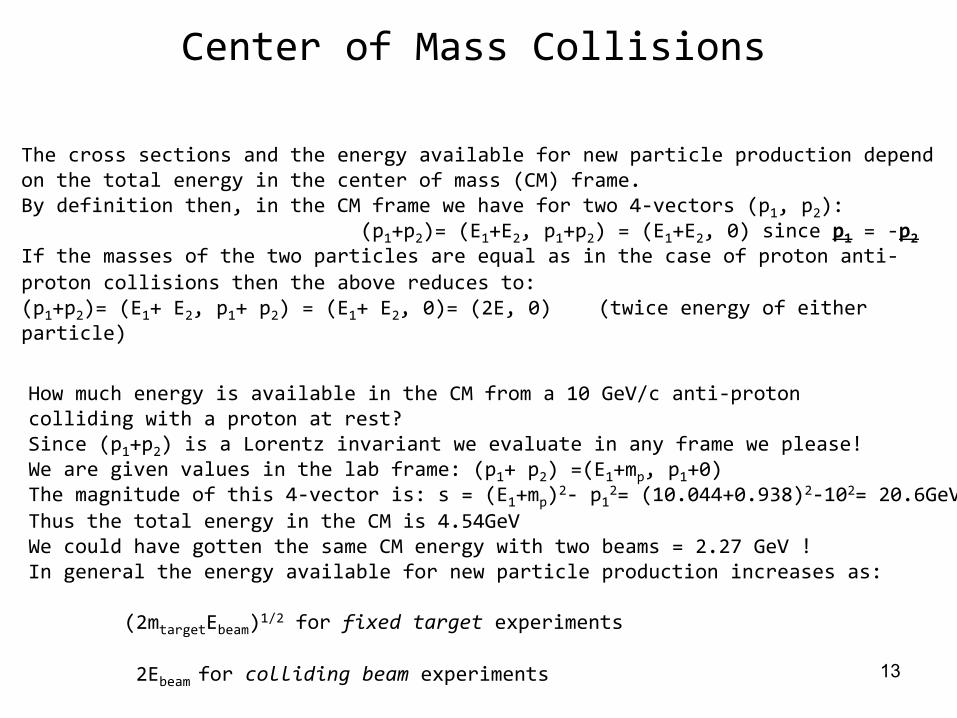
Center of Mass Collisions

The cross sections and the energy available for new particle production depend on the total energy in the center of mass (CM) frame. By definition then, in the CM frame we have for two 4-‐vectors (p1, p2): (p1+p2)= (E1+E2, p1+p2) = (E1+E2, 0) since p1 = -‐p2 If the masses of the two particles are equal as in the case of proton anti-‐proton collisions then the above reduces to: (p1+p2)= (E1+ E2, p1+ p2) = (E1+ E2, 0)= (2E, 0) (twice energy of either particle)

How much energy is available in the CM from a 10 GeV/c anti-‐proton colliding with a proton at rest? Since (p1+p2) is a Lorentz invariant we evaluate in any frame we please! We are given values in the lab frame: (p1+ p2) =(E1+mp, p1+0) The magnitude of this 4-‐vector is: s = (E1+mp)2-‐ p12= (10.044+0.938)2-‐102= 20.6GeV2 Thus the total energy in the CM is 4.54GeV We could have gotten the same CM energy with two beams = 2.27 GeV ! In general the energy available for new particle production increases as:

(2mtargetEbeam)1/2 for fixed target experiments

2Ebeam for colliding beam experiments

colliding beams are more efficient for heavy particle production

13

14

Types of collisions •  The available energy for the reactions is the

energy of the projectile-‐target system on in Center of Mass reference frame.

•  The minimum E to create a particle of mass M is: •  Fixed target: E > M2c2/2mt, where mt is the target

mass •  "Head on": E> Mc2/2 •  For example to create a W boson (M≈80 GeV/c2)

with p collisions on a fixed target (m≈1 GeV/c2) E > M2c2/2m = 802/(2*1) = 3200 GeV: difficult!

•  While in a head-‐on collision of protons (or p-‐antip), E > Mc2/2 = 40 GeV (each) à easy to do! –  All the beam energy is available for reactions

Even More Relativistic Kinematics In the early 1950’s many labs were trying to find evidence of the anti-‐proton. At Berkeley a new proton accelerator (BEVATRON) was being designed for this purpose. Assuming fixed target proton-‐proton collisions would be used to create the antiproton what energy proton beam (Eb) is necessary ? The simplest reaction that conserves all the necessary quantities (energy, momentum, electric charge, baryon number) is:

p p → p p p p with p = anti-proton

The total energy in the CM is given by: (pb+pt)2 the sum of the 4-‐vectors of the beam and target proton (assumed to be at rest): (pb+pt)2 =(Eb+mp, pb)2= mb2+mt2+2mtEb=2mp2+2mpEb The trick now is to remember that (pb+pt)2 is Lorentz invariant and can be evaluated in any frame we choose. The most convenient frame is the one where all the final state particles are produced at rest. Here we have: (pb+pt)2initial =(Eb+mp, pb)2= (pb+pt)2final = (4mp)2 2mp2+2mpEb = (4mp)2 Eb = 7mp= 6.6 GeV The anti-‐proton was discovered at Berkeley in 1955 (Nobel Prize 1959) 15

Mass of Short-‐lived Particle •  We can’t see short-‐lived particles (that is

they don’t reach the detectors) but rather their decay products

•  From invariant mass of its decay products, e.g. 2-‐body:

•  How to measure ma?

mc,Ec

ma

mb,Eb

θbc

16

•  Initial invariant mass s = ma2 •  Final invariant mass = •  If Eb, Ec >> mc , mc then Eb, Ec~ pb, pc •  So,

•  If we measure Eb,Ec and the angle, we can determine the mass of the parent particle

(Eb +Ec )2 − ( pb +

pc )2

( )θ abcba CosEEm −= 122

Higgs boson discovery in γγ decay channel

17 ( )θ abcba CosEEm −= 122

Interaction Rates and Cross-‐sections

• No matter what experiment, at the end, one ends up counting particles

• Experiments measure rates of reactions – these depend on both – “kinematics” e.g. energy available to final state particles, and

– “dynamics”, e.g. strength of interaction, propagator factors etc.

18

Cross section σ • Cross section gives the probability for a given process to occur

• Cross section incorporates: –  Strength of underlying interaction (vertices) –  Propagators for virtual exchange factors –  Phase space factors (available energy) –  Does not depend on rate of incoming particles.

• Called the “cross-‐section” because it has units of area. –  Normally quoted in units of barns (10-‐28m2) … or multiples eg. nanobarns (nb), picobarns (pb)

19

•  Formally, the cross-‐section is defined in the following manner: Consider a beam of particles 1 incident upon a target particle 2. Assume that the beam is much broader than the target and that the particles in the beam are uniformly distributed in space and time.

•  We can speak of a flux F of incident particles (cm-‐2s-‐1). •  Now look at the number Ns of particles scattered into the solid

angle dΩ per unit time, dNs/dΩ . •  Because of the randomness of the impact parameters, this number

will fluctuate over different finite periods of measuring time. However, if we average many finite measuring periods, this number will tend towards a fixed dNs/dΩ where Ns is the average number scattered per unit time. The differential cross section is then defined as the ratio

20

Cross section σ

•  dσ/dΩ is the average fraction of the particles scattered into

dΩ per unit time per unit flux F.

21

•  Note that because of the dimensions of F, dσ has dimensions of area, which leads to the heuristic interpretation of dσ as the geometric cross sectional area of the target intercepting the beam. That fraction of the flux incident on this area will then obviously interact while all those missing da will not. This is only a visual aid, however, and should in no way be taken as a real measure of the physical dimensions of the target.

Cross section σ

22

Cross-‐Section – “physical” interpretation σ is used to measure the probability of interactions between elementary particles.

•  If we play dartboard, the important parameter is the target dimension, that is the surface area that incident dart beam sees.

•  Similarly, if we shoot an electron beam on a H tank, the important parameter is the proton dimension, that is the surface area seen by the incident beam. But the proton has not a well defined section; the more the e-‐ gets close, the higher is the interaction probability. The cross section depends on projectile and target species, on energy, spin,… . –  elastic cross section (if the energy is low we will have only e+pàe+p) –  anelastic cross section (if the energy is enough we can have e+pàe+p+γ

or e+pàe+p+π etc )

–  1 barn (b) =10-‐24 cm2

For a linear momentum in the lab of 10 GeV/c we have: •  σt ( π+p ) ~ 25 mb (forte) •  σt ( γp ) ~ 100 µb (e.m.) •  σt ( νp ) ~ 0.1 pb (debole)

Cross-‐Section – “physical” interpretation

•  Can be thought of as an effective area centred on the target – if the incident particle passes through this area an interaction occurs. –  Physical picture only realistic for short range interactions. (target behaves like a featureless extended ball)

–  For long range interactions, like EM, integrated cross-‐section is infinite.

23

•  In real situations, the target is usually a slab of material containing many scattering centers and it is desired to know how many interactions occur on the average.

•  Assuming that the target centers are uniformly distributed and the slab is not too thick so that the likelihood of one center sitting in front of another is low, the number of centers per unit perpendicular area which will be seen by the beam is then Ndx where N is the density of centers and dx is the thickness of the material along the direction of the beam. If the beam is broader than the target and A is the total perpendicular area of the target, the number of incident particles which are eligible for an interaction is then FA. The average number scattered into dΩ per unit time is then

25

If the beam is smaller than the target, then we need only set A equal to the area covered by the beam. Then FA = ninc, the total number of incident particles per unit time. In both cases, now, if we divide by FA, we have the probability for the scattering of a single particle in a thickness dx, Prob. of interaction in dx = Nσ dx

Cross-‐section and Interaction rate.

• For fixed target, with a target larger than the beam

• W=rntLσ – W =interaction rate (# interactions/s) – r =rate of incoming particles (# part/s) – nt =number density of target particles (# part m-‐3)

– L = thickness of target (m) – σ = cross-‐section for interaction (m2)

L

r

26

Cross-‐section and Interaction rate quick calc

•  Given a single target, by definition of x-‐section, all the particles in the volume σdx = σvdt will interact with target.

•  If the projectile particles have density np, then the # interactions is dN= npσvdt.

•  If there is a nbr density of targets nt, the interacion rate per unit of volume is

dN/dVdt = ntnpσv •  If the interaction volume is V = S L, with S

section of projectile beam and L target thickness, then interaction rate is W = nt np σ v S L, but the rate of incident part is r = nt v S è W=r nt L σ

27

Cross-‐section and Interaction rate.

• W = nt np σ c S L • For fixed target, in terms of particle flux, J = np c

• W=J n σ – W = interaction rate – J = Flux: particles per unit area per unit time.

– n = total number density of particles in target.

– σ = cross-‐section for interaction 28

29

Sezione d’urto •  Esempio numerico: p-‐ pà π0 n

–  Np = 107 particelle incidenti a burst ( impulso dell’acceleratore)

–  1 burst ogni 10 s –  8 giorni di presa dati (Ndays) –  Bersaglio di Be (ρ =1.8 gr/cm3) L=10 cm –  Dati raccolti 7.49x1010 La relazione da usare e’: W=r nt L σ Se prendiamo dati per un tempo dT, il numero di interazioni e’ Nrac = WdT = (rdT) nt L σ, rdT = Nfascio = (Np * 86400/10) * Ndays Ci serve in nr. di protoni del bersaglio: La densita’ di numero di atomi di Be e’ nBe = ρ/mBe La massa mBe si ottiene dalla relazione mBe = Mmol/NA = A/NA, Mmol =

massa molare (Kg/mol) = A kg/mol à nBe = ρNA/A, Il numero atomico e’ Z quindi ci sono np = ZnBe= ρNA(Z/A) protoni,

con Z/A = 4/9 per unita’ di volume σT=(Nrac/Nfascio)x(1/nA) (Nrac=7.49x1010 , Nfascio=6.9120x1011)

nA = Lnp (numero di protoni/cm2 visti dal fascio) σT = (7.49x1010)/(69120x107x48.18x1023)~2.25x10-‐26 cm2=22.5 mb

Colliding Beam Interaction Rate •  In a colliding beam accelerator, particles in each

beam stored in bunches (see accelerators, later). –  Bunches pass through each other at interaction point, with

a frequency f –  Have an effective overlap area, A è interaction rate is

–  Can express in terms of beam currents I=nf

•  Factors n1n2f/A normally called the Luminosity, L

σLW =

σAfnnW 21=

σAfIIW 21=

30

Colliding Beam Interaction Rate quick calc

•  In one revolution, a particle of the bunch 1 "sees" a bunch of N2 particles, distributed over an effective surface A à sees a particle density of N2/A.

•  Since there are N1 particles, circulating with freq f, the # of encounters per unit of time and surface is (N2/A)fN1

•  In each encounter, the probability for a given process to occur is σ è

σAfnnW 21=

31

Differential Cross-‐section, dσ

• We have just defined the total cross-‐section, σ, related to the probability that an interaction of any kind occurred.

• Often interested in the probability of an interaction with a given outcome (e.g. particle scatters through a given angle or with a given energy)

32

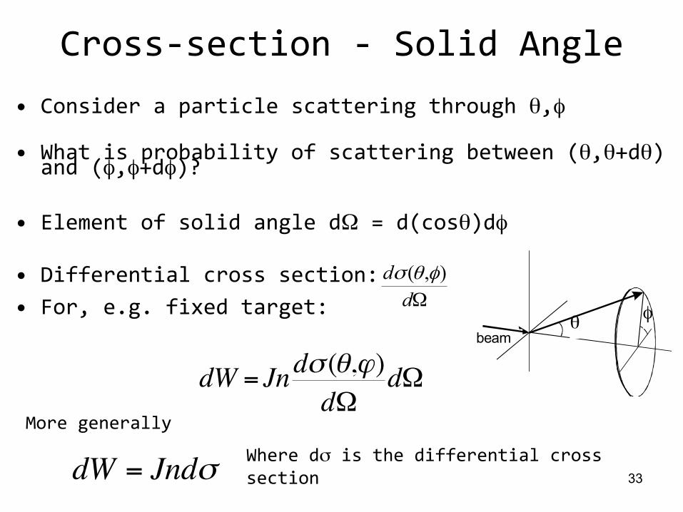
Cross-‐section -‐ Solid Angle •  Consider a particle scattering through θ,φ

•  What is probability of scattering between (θ,θ+dθ) and (φ,φ+dφ)?

•  Element of solid angle dΩ = d(cosθ)dφ

•  Differential cross section: •  For, e.g. fixed target:

θ φbeam

Ωdd ),( φθσ

dW = Jndσ (θ,ϕ)dΩ

dΩ

33

More generally

dW = Jndσ Where dσ is the differential cross section

Differential àTotal Cross-section

•  To get from differential to total cross-‐section:

•  With unpolarized beams – no dependence on φ -‐ integrate to get dσ(θ)/dΩ

•  If measuring some other variable ( e.g. final state energy, E) other differential cross-‐sections, e.g:

∫ ∫π

− Ω

φθσθφ=σ

2

0

1

1

),(cosd

ddd

21

2

dEdEd σ

34

ParticleDetectors Lecture 3 140318

Documents

Transcript of ParticleDetectors Lecture 3 140318