Relativistic Particle Acceleration in a Developing Turbulence
Upload
franklin-simmonsCategory
view
221download
1
Particle Transport (and a little Particle Acceleration)
Gordon EmslieOklahoma State University

Evidence for Energetic ParticlesEvidence for Energetic Particles
Particles escaping into interplanetary space
Hard X-ray emission (electrons)
Gamma-ray emission (electrons and ions)
Radio emission (electrons)
Will focus mostly on electrons in this talk

Bremsstrahlung ProcessBremsstrahlung Process

Inversion of Photon Spectra
I()= K F(E) (,E) dE
(,E) = /E
J()= I() = K G(E) dE
G(E) = -(1/K) dJ()/d
G(E) ~ J()

Inversion of Photon Spectra
I()= K F(E) (,E) dE
(,E) = /E
J()= I() = K G(E) dE
G(E) = -(1/K) dJ()/d
G(E) ~ J()
Key point!Key point!
Emission process is straightforward, and so it is easy to ascertain the number of electrons from the observed number of photons!

Required Particle Required Particle Fluxes/Fluxes/CurrentsCurrents//PowersPowers//EnergiesEnergies
(Miller et al. 1997; straightforwardly proportional to observed photon flux)
ElectronsElectrons1037 s-1 > 20 keV1018 Amps3 1029 ergs s-1 for 100 s = 3 1031 ergs
IonsIons1035 s-1 > 1 MeV1016 Amps2 1029 ergs s-1 for 100 s = 2 1031 ergs

Order-of-Magnitude Energetics

Electron Number ProblemElectron Number Problem
1037 s-1 > 20 keV
Number of electrons in loop = nV ~ 1037
All electrons accelerated in 1 second!
Need replenishment of acceleration region!

Electron Current ProblemElectron Current ProblemSteady-state (Ampère):
B = oI/2r ~ (10-6)(1018)/108 = 104 T = 108 G
(B2/8) V ~ 1041 ergs!
Transient (Faraday):
V = (ol) dI/dt = (10-6)(107)(1018)/10 ~ 1018 V!!
So either(1) currents must be finely filamented; or(2) particle acceleration is in random directions

An Acceleration PrimerAn Acceleration Primer
F = qEpart; Epart = Elab + vpart B
• Epart large-scale coherent acceleration
• Epart small-scale stochastic acceleration

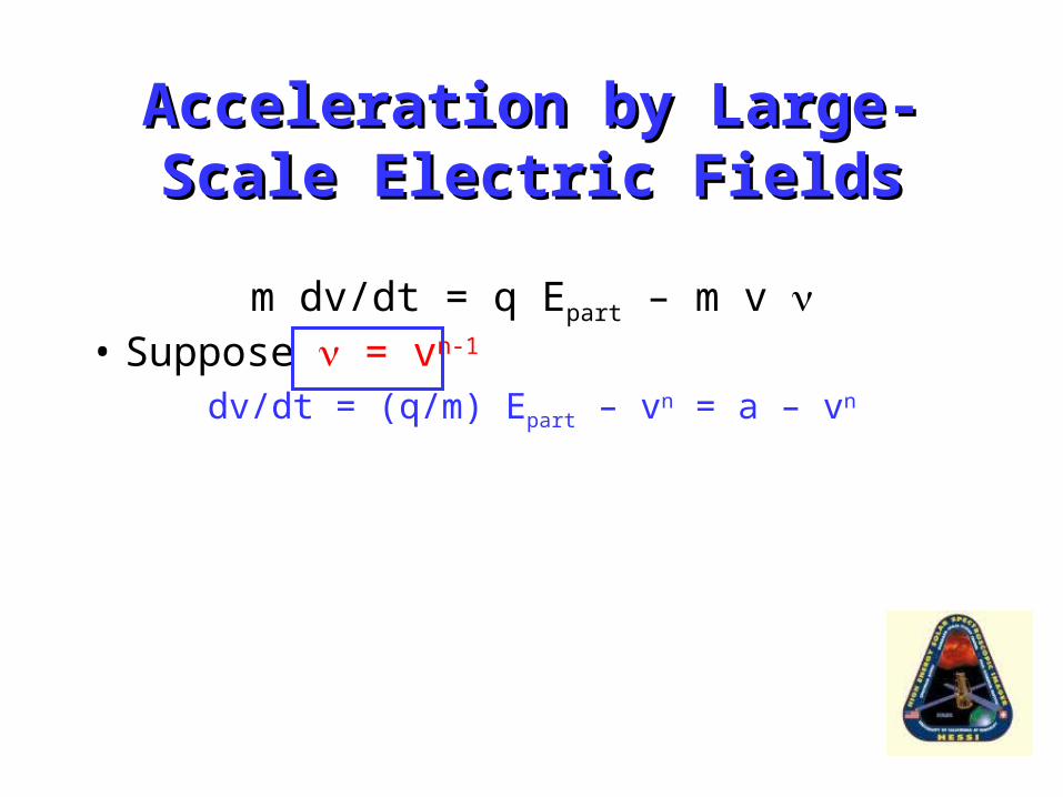
Acceleration by Large-Scale Acceleration by Large-Scale Electric FieldsElectric Fields
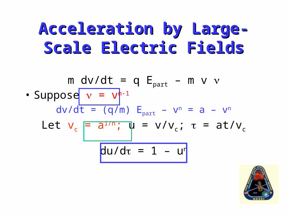
m dv/dt = q Epart – m v • Suppose = a vn-1
dv/dt = (q/m) Epart – a vn = g – a vn
Let vc = (g/a)1/n; u = v/vc; = gt/vc
du/d = 1 – un
• For air drag, ~v (n = 2)• For electron in plasma, ~1/v3 (n = -2)
Acceleration by Large-Scale Acceleration by Large-Scale Electric FieldsElectric Fields
m dv/dt = q Epart – m v • Suppose = vn-1
dv/dt = (q/m) Epart – vn = a – vn
Let vc = g1/n; u = v/vc; = gt/vc
du/d = 1 – un
• For air drag, ~v (n = 2)• For electron in plasma, ~1/v3 (n = -2)
Acceleration by Large-Scale Acceleration by Large-Scale Electric FieldsElectric Fields
m dv/dt = q Epart – m v • Suppose = vn-1
dv/dt = (q/m) Epart – vn = a – vn
Let vc = a1/n; u = v/vc; = at/vc
du/d = 1 – un
• For air drag, ~v (n = 2)• For electron in plasma, ~1/v3 (n = -2)
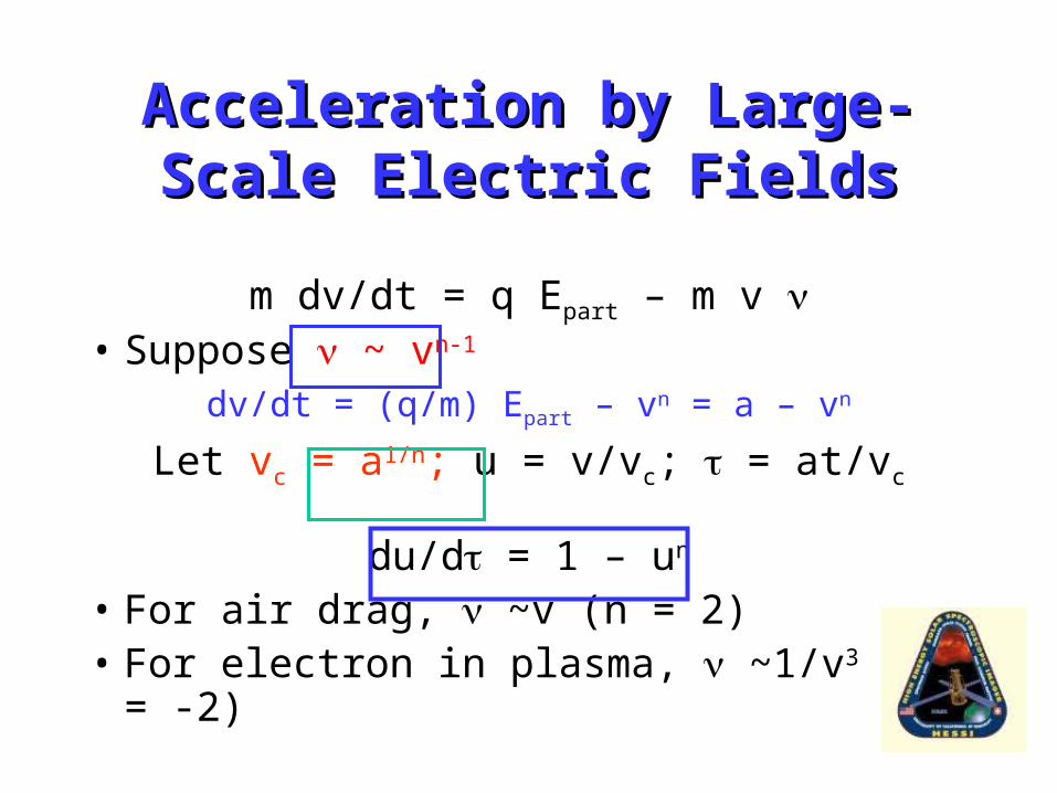
Acceleration by Large-Scale Acceleration by Large-Scale Electric FieldsElectric Fields
m dv/dt = q Epart – m v • Suppose ~ vn-1
dv/dt = (q/m) Epart – vn = a – vn
Let vc = a1/n; u = v/vc; = at/vc
du/d = 1 – un
• For air drag, ~v (n = 2)• For electron in plasma, ~1/v3 (n = -2)

Acceleration TrajectoriesAcceleration Trajectories
u
du/ddu/d = 1 - un

Acceleration TrajectoriesAcceleration Trajectories
u
du/d
1
1
n>0
du/d = 1 - un

Acceleration TrajectoriesAcceleration Trajectories
u
du/d
1
1
n<0
n>0
du/d = 1 - un

Acceleration TrajectoriesAcceleration Trajectories
u
du/d
1
1
u increasing
n<0
n>0
du/d = 1 - un
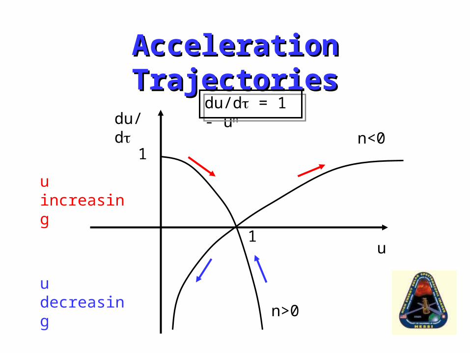
Acceleration TrajectoriesAcceleration Trajectories
u
du/d
1
1
u increasing
u decreasing
n<0
n>0
du/d = 1 - un
Acceleration TrajectoriesAcceleration Trajectories
u
du/d
1
1
u increasing
u decreasing
n<0
n>0, stable
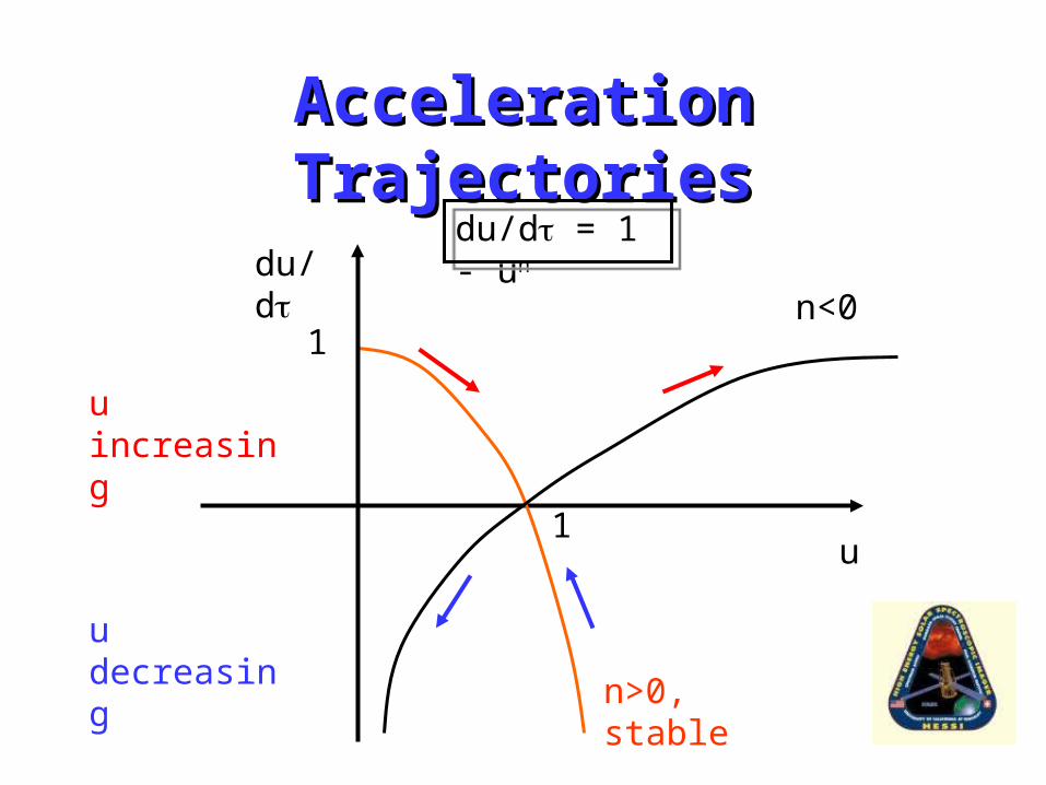
du/d = 1 - un

Acceleration TrajectoriesAcceleration Trajectories
u
du/d
1
1
u increasing
u decreasing
n<0, unstable
n>0, stable
du/d = 1 - un
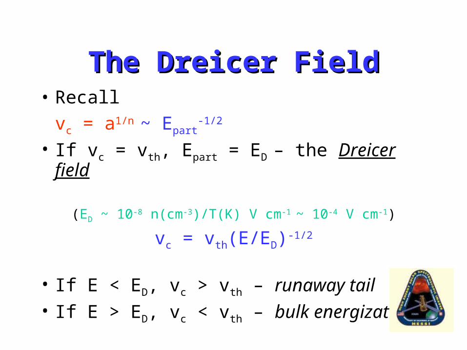
The Dreicer FieldThe Dreicer Field• Recall
vc = a1/n ~ Epart-1/2
• If vc = vth, Epart = ED – the Dreicer field
(ED ~ 10-8 n(cm-3)/T(K) V cm-1 ~ 10-4 V cm-1)
vc = vth(E/ED)-1/2
• If E < ED, vc > vth – runaway tail• If E > ED, vc < vth – bulk energization

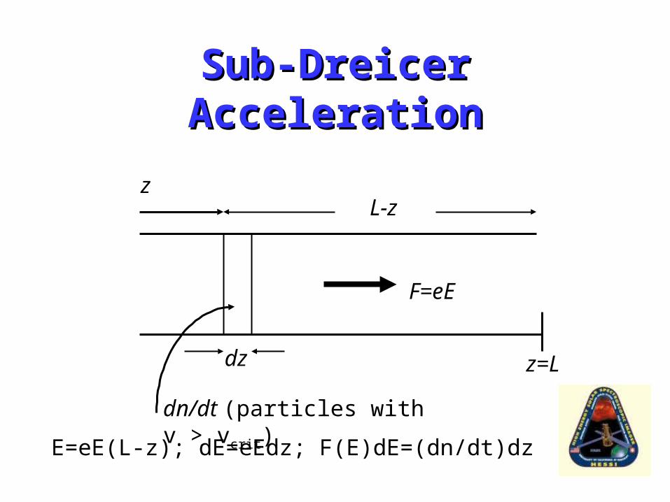
Sub-Dreicer AccelerationSub-Dreicer Acceleration
L-z
dz
F=eE
z
dn/dt (particles with v > vcrit)
z=L
Sub-Dreicer AccelerationSub-Dreicer Acceleration
L-z
dz
F=eE
z
dn/dt (particles with v > vcrit)
z=L
E=eE(L-z); dE=eEdz; F(E)dE=(dn/dt)dz
→ F(E)=(1/e)(dn/dt)

Sub-Dreicer AccelerationSub-Dreicer Acceleration
L-z
dz
F=eE
z
dn/dt (particles with v > vcrit)
z=L
Emergent spectrum is flat!
E=eE(L-z); dE=eEdz; F(E)dE=(dn/dt)dz
→ F(E)=(1/eE )(dn/dt)
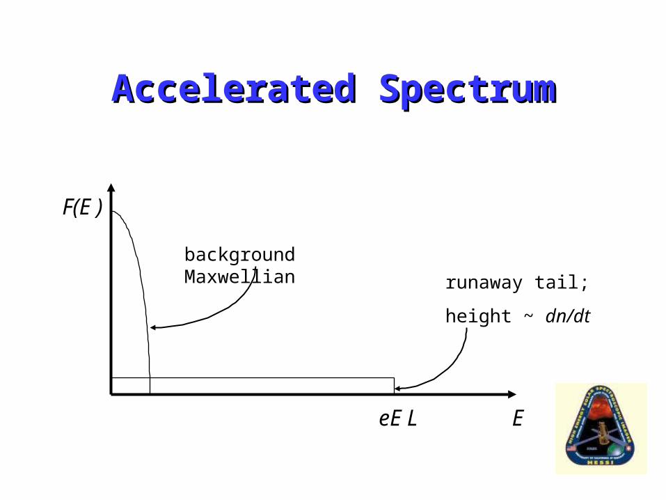
Accelerated SpectrumAccelerated Spectrum
F(E )
EeE L
runaway tail;
height ~ dn/dt
background Maxwellian

Computed Runaway DistributionsComputed Runaway Distributions
(Sommer 2002, Ph.D. dissertation, UAH)

Photon Spectrum

Accelerated SpectrumAccelerated Spectrum
•Predicted spectrum is flat
•Observed spectrum is ~ power law
•Need many concurrent acceleration regions, with range of E and L

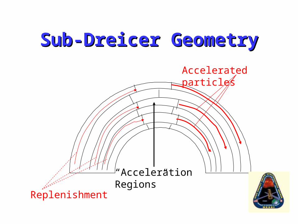
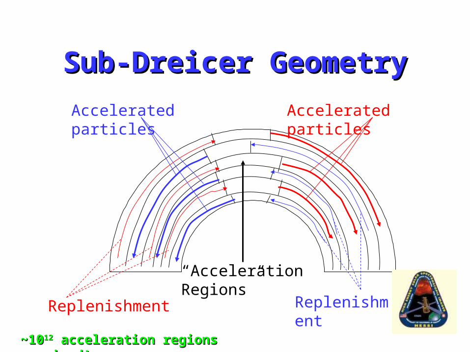
Sub-Dreicer GeometrySub-Dreicer Geometry
“Acceleration Regions”
Accelerated particles

Sub-Dreicer GeometrySub-Dreicer Geometry
“Acceleration Regions”
Replenishment
Accelerated particles
Sub-Dreicer GeometrySub-Dreicer Geometry
“Acceleration Regions”
Replenishment
Accelerated particles

Sub-Dreicer GeometrySub-Dreicer Geometry
“Acceleration Regions”
Accelerated particles
Replenishment
Accelerated particles
Replenishment
Sub-Dreicer GeometrySub-Dreicer Geometry
“Acceleration Regions”
Accelerated particles
Replenishment Replenishment
Accelerated particles
~10~101212 acceleration regions required! acceleration regions required!
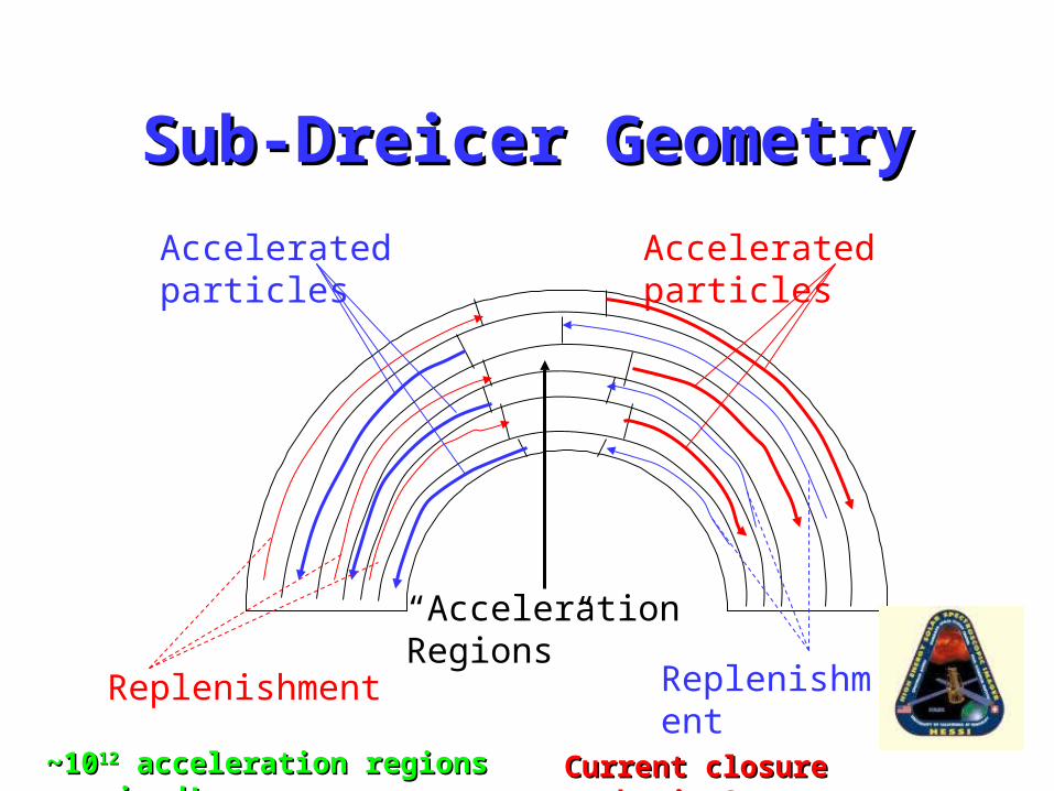
Sub-Dreicer GeometrySub-Dreicer Geometry
“Acceleration Regions”
Accelerated particles
Replenishment
Accelerated particles
~10~101212 acceleration regions required! acceleration regions required! Current closure mechanism?Current closure mechanism?
Replenishment

Sub-Dreicer AccelerationSub-Dreicer Acceleration
• Long (~109 cm) acceleration regions• Weak (< 10-4 V cm-1) fields• Small fraction of particles accelerated• Replenishment and current closure are challenges• Fundamental spectral form is flat• Need large number of current channels to account
for observed spectra and to satisfy global electrodynamic constraints

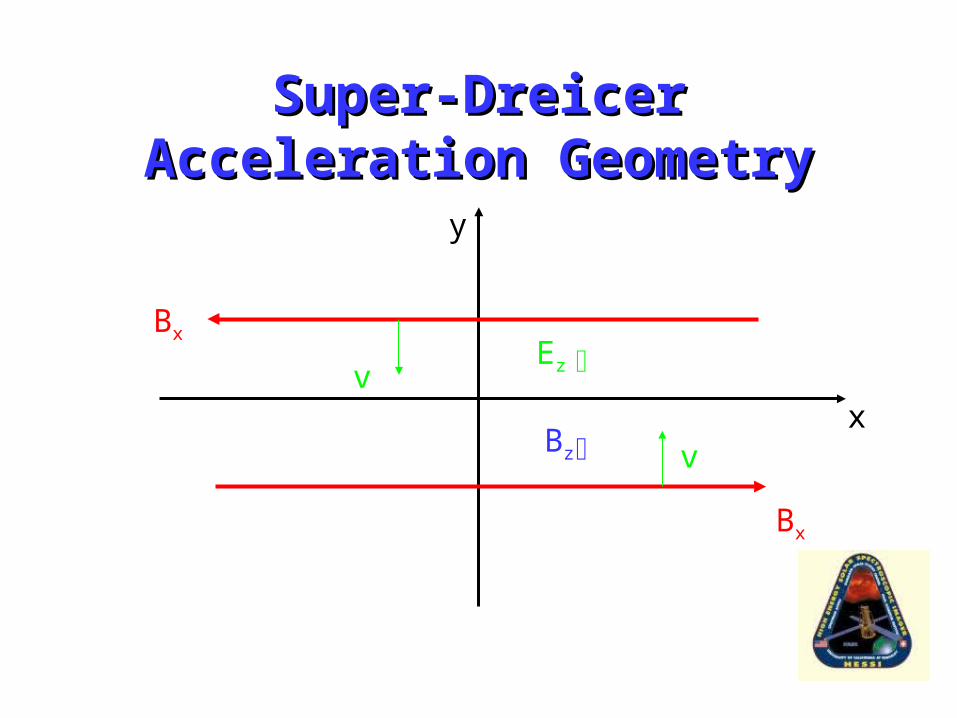
Super-Dreicer AccelerationSuper-Dreicer Acceleration
• Short-extent (~105 cm) strong (~1 V cm-1) fields in large, thin (!) current sheet
Super-Dreicer Acceleration Super-Dreicer Acceleration GeometryGeometry
x
y

Super-Dreicer Acceleration Super-Dreicer Acceleration GeometryGeometry
x
y
Bx
Bx
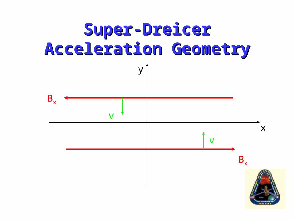
Super-Dreicer Acceleration Super-Dreicer Acceleration GeometryGeometry
x
y
Bx
Bx
v
v

Super-Dreicer Acceleration Super-Dreicer Acceleration GeometryGeometry
x
y
Bx
Bx
Ez v
v
Ez = – v B
Super-Dreicer Acceleration Super-Dreicer Acceleration GeometryGeometry
x
y
Bx
Bx
Ez
Bz
v
v

Super-Dreicer Acceleration Super-Dreicer Acceleration GeometryGeometry
x
y
Bx
Bx
Ez
Bz
v
v
Field-aligned acceleration
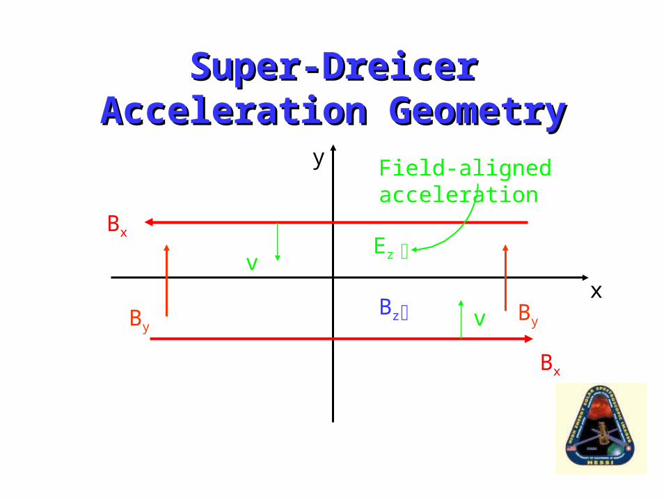
Super-Dreicer Acceleration Super-Dreicer Acceleration GeometryGeometry
x
y
Bx
Bx
Ez
Bz
v
vByBy
Field-aligned acceleration
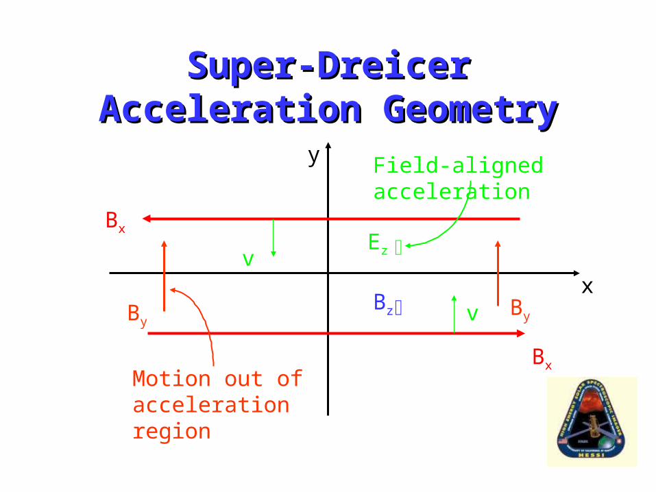
Super-Dreicer Acceleration Super-Dreicer Acceleration GeometryGeometry
x
y
Bx
Bx
Ez
Bz
v
vByBy
Field-aligned acceleration
Motion out of acceleration region

Super-Dreicer AccelerationSuper-Dreicer Acceleration
• Short (~105 cm) acceleration regions• Strong (> 10 V cm-1) fields• Large fraction of particles accelerated• Can accelerate both electrons and ions• Replenishment and current closure are
straightforward• No detailed spectral forms available• Need very thin current channels – stability?
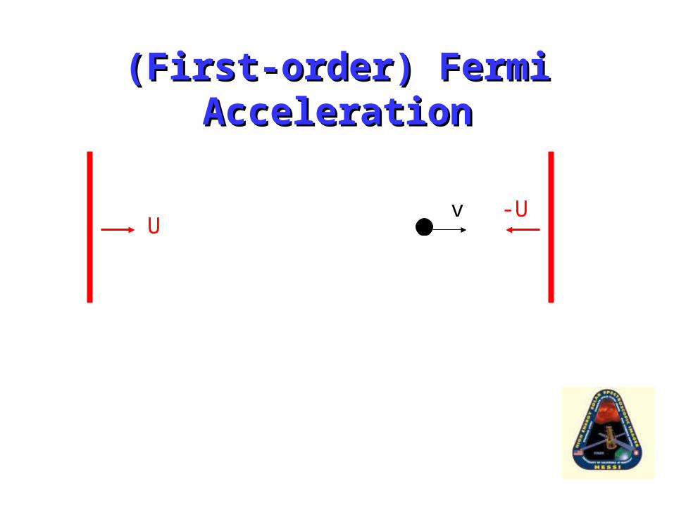
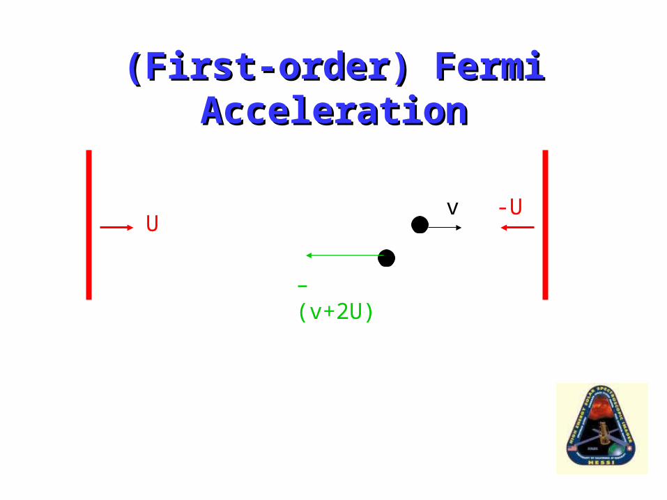
(First-order) Fermi Acceleration(First-order) Fermi Acceleration
U-Uv
(First-order) Fermi Acceleration(First-order) Fermi Acceleration
U-Uv
– (v+2U)
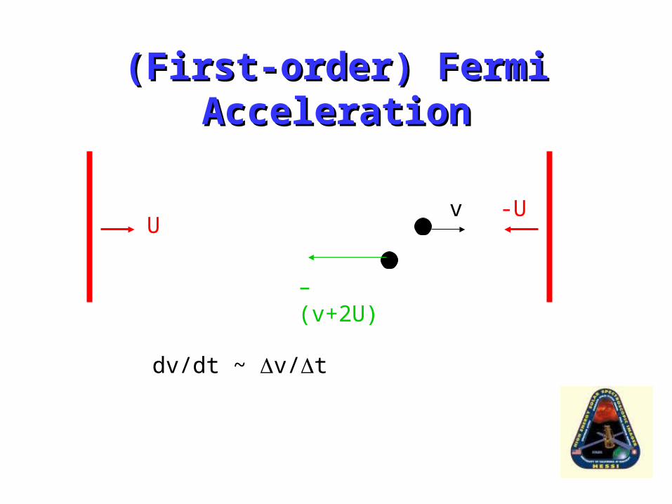
(First-order) Fermi Acceleration(First-order) Fermi Acceleration
U-Uv
– (v+2U)
dv/dt ~ v/t
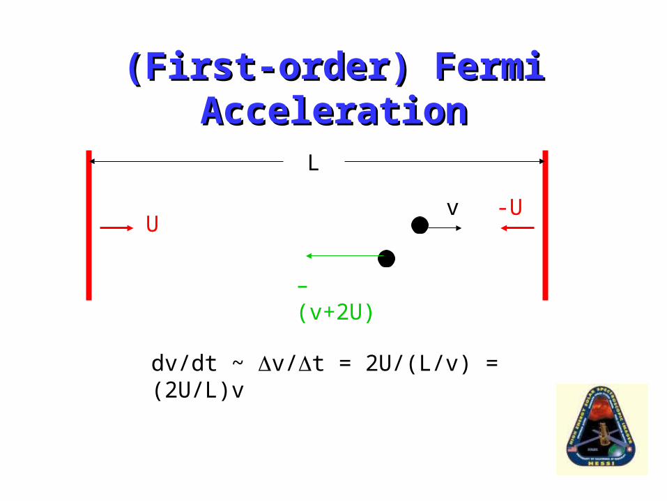
(First-order) Fermi Acceleration(First-order) Fermi Acceleration
U-Uv
– (v+2U)
dv/dt ~ v/t = 2U/(L/v) = (2U/L)v
L
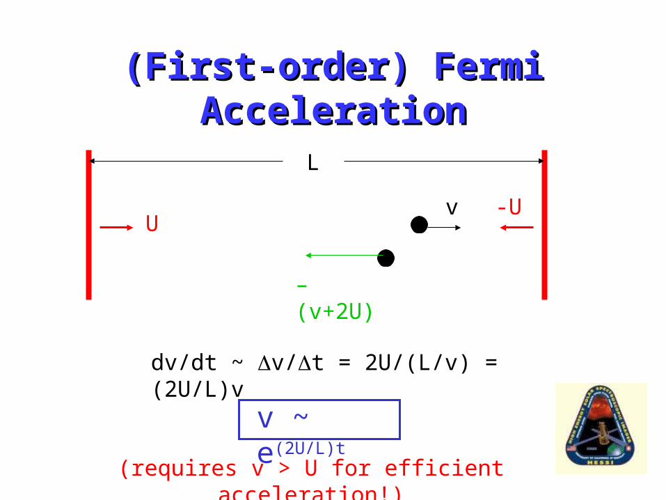
(First-order) Fermi Acceleration(First-order) Fermi Acceleration
U-Uv
– (v+2U)
dv/dt ~ v/t = 2U/(L/v) = (2U/L)v
v ~ e(2U/L)t
L
(requires v > U for efficient acceleration!)

Second-order Fermi AccelerationSecond-order Fermi Acceleration
• Energy gain in head-on collisions
• Energy loss in “overtaking collisions”
Second-order Fermi AccelerationSecond-order Fermi Acceleration
• Energy gain in head-on collisions
• Energy loss in “overtaking collisions”
BUT number of head-on collisions exceeds number of overtaking collisions
→ Net energy gain!

Stochastic Fermi AccelerationStochastic Fermi Acceleration(Miller, LaRosa, Moore)(Miller, LaRosa, Moore)
• Requires the injection of large-scale turbulence and subsequent cascade to lower sizescales
• Large-amplitude plasma waves, or magnetic “blobs”, distributed throughout the loop
• Adiabatic collisions with converging scattering centers give 2nd-order Fermi acceleration (as long as v > U! )
Stochastic Fermi AccelerationStochastic Fermi Acceleration
• Thermal electrons have v>vA and are efficiently accelerated immediately
• Thermal ions take some time to reach vA and hence take time to become efficiently accelerated

Stochastic Acceleration
t = 0 – 0.1 s
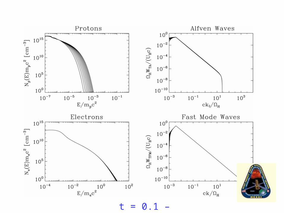
t = 0.1 – 0.2 s

t = 0.2 – 1.0 s

T = 2 – 4 s Equilibrium

Stochastic AccelerationStochastic Acceleration
• Accelerates both electrons and ions
• Electrons accelerated immediately
• Ions accelerated after delay, and only in long acceleration regions
• Fundamental spectral forms are power-laws
Electron vs. Ion Acceleration and Transport
• If ion and electron acceleration are produced by the same fundamental process, then the gamma-rays produced by the ions should be produced in approximately the same location as the hard X-rays produced by the electrons

Observations: 2002 July 23 Flare
WRONG!!!
WRONG!!!
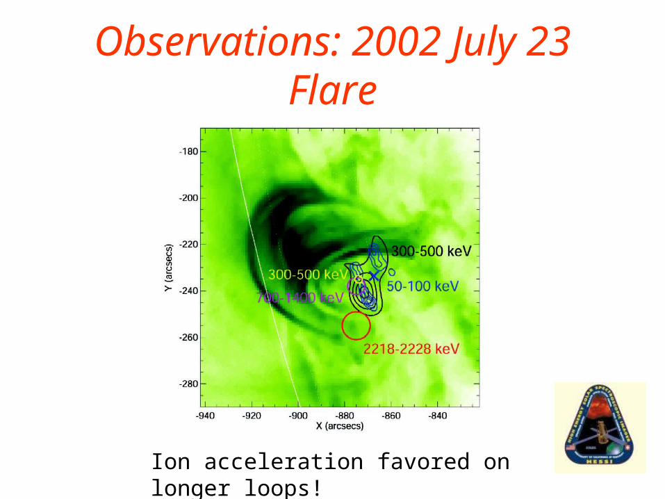
Observations: 2002 July 23 Flare
Ion acceleration favored on longer loops!

Particle TransportParticle Transport
Cross-section
dE/dt ~ n v E

Particle TransportParticle Transport
Cross-section
dE/dt = n v E

Particle TransportParticle Transport
Cross-section
dE/dt = n v E
erg s-1 cm-3 erg
cm s-1

Particle TransportParticle Transport
Cross-section
dE/dt = n v E
erg s-1
cm2
cm-3 erg
cm s-1

Coulomb collisionsCoulomb collisions
= 2e4Λ/E2;– Λ = “Coulomb logarithm” ~ 20)
• dE/dt = -(2e4Λ/E) nv = -(K/E) nv
• dE/dN = -K/E; dE2/dN = -2K
• E2 = Eo2 – 2KN
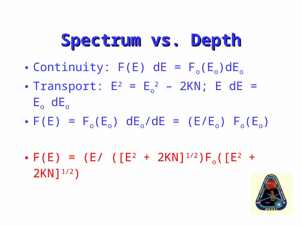
Spectrum vs. DepthSpectrum vs. Depth
• Continuity: F(E) dE = Fo(Eo)dEo
• Transport: E2 = Eo2 – 2KN; E dE = Eo dEo
• F(E) = Fo(Eo) dEo/dE = (E/Eo) Fo(Eo)
• F(E) = (E/ ([E2 + 2KN]1/2)Fo([E2 + 2KN]1/2)
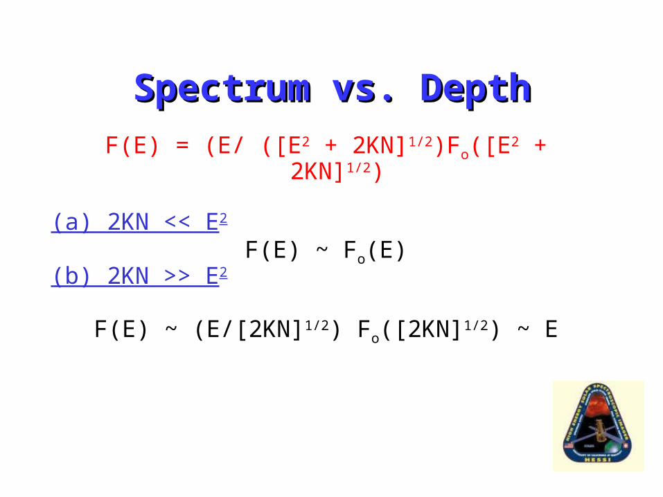
Spectrum vs. DepthSpectrum vs. Depth
F(E) = (E/ ([E2 + 2KN]1/2)Fo([E2 + 2KN]1/2)
(a) 2KN << E2
F(E) ~ Fo(E)(b) 2KN >> E2
F(E) ~ (E/[2KN]1/2) Fo([2KN]1/2) ~ E
Also,v f(v) dv = F(E) dE f(v) = m F(E)

Spectrum vs. DepthSpectrum vs. Depth
F(E) = (E/ ([E2 + 2KN]1/2)Fo([E2 + 2KN]1/2)
(a) 2KN << E2
F(E) ~ Fo(E)(b) 2KN >> E2
F(E) ~ (E/[2KN]1/2) Fo([2KN]1/2) ~ E
Also,v f(v) dv = F(E) dE f(v) = m F(E)

Spectrum vs. DepthSpectrum vs. Depth
Resulting photon spectrum gets harder with depth!

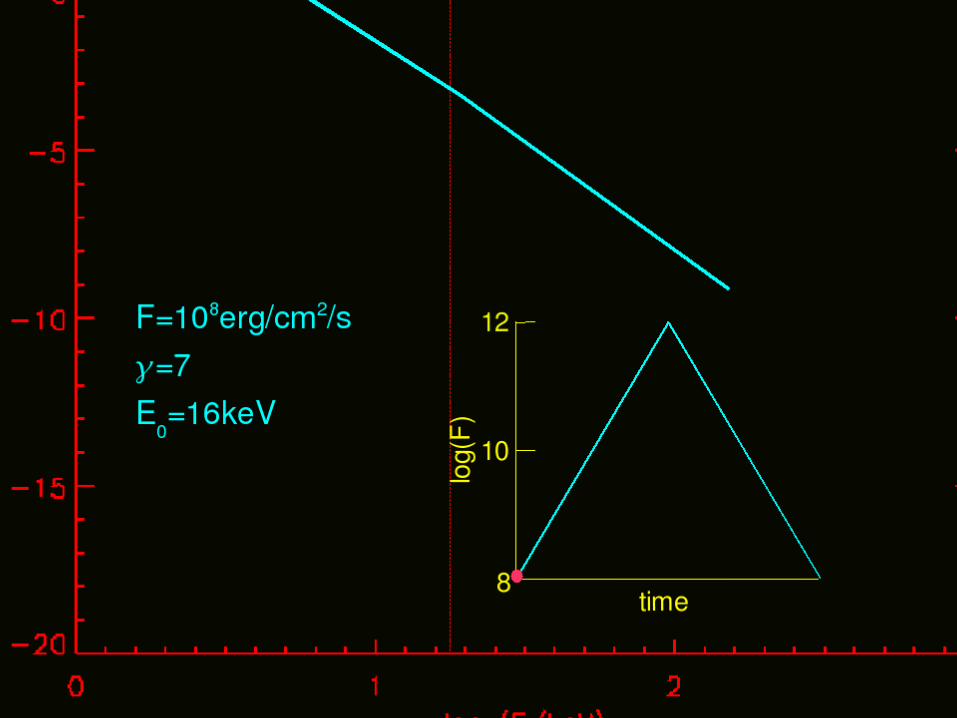
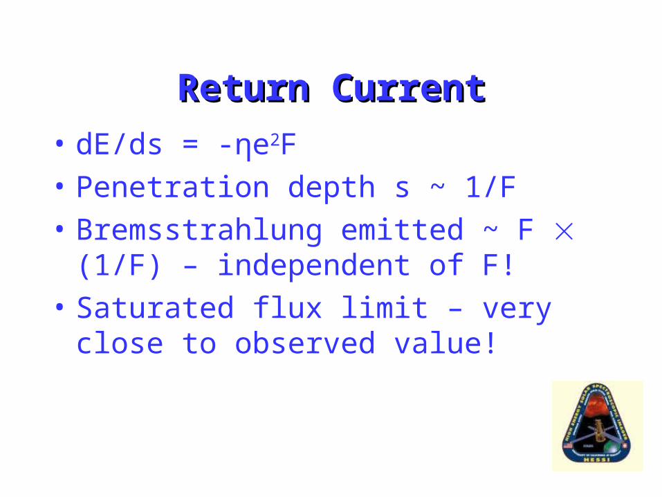
Return CurrentReturn Current
• dE/ds = -eE, E = electric field
• Ohm’s Law: E = η j = ηeF, F = particle flux
• dE/ds = -ηe2F
• dE/ds independent of E: E = Eo – e2 ∫ η F ds
– note that F = F[s] due to transport and η = η(T)
Return CurrentReturn Current
• Zharkova results
Return CurrentReturn Current
• dE/ds = -ηe2F• Penetration depth s ~ 1/F• Bremsstrahlung emitted ~ F (1/F) –
independent of F!
• Saturated flux limit – very close to observed value!

Magnetic MirroringMagnetic Mirroring• F = - dB/ds; = magnetic moment• Does not change energy, but causes
redirection of momentum• Indirectly affects energy loss due to other
processes, e.g. – increase in pitch angle reduces flux F and so
electric field strength E– Penetration depth due to collisions changed.

Observational Tests of TransportObservational Tests of Transport
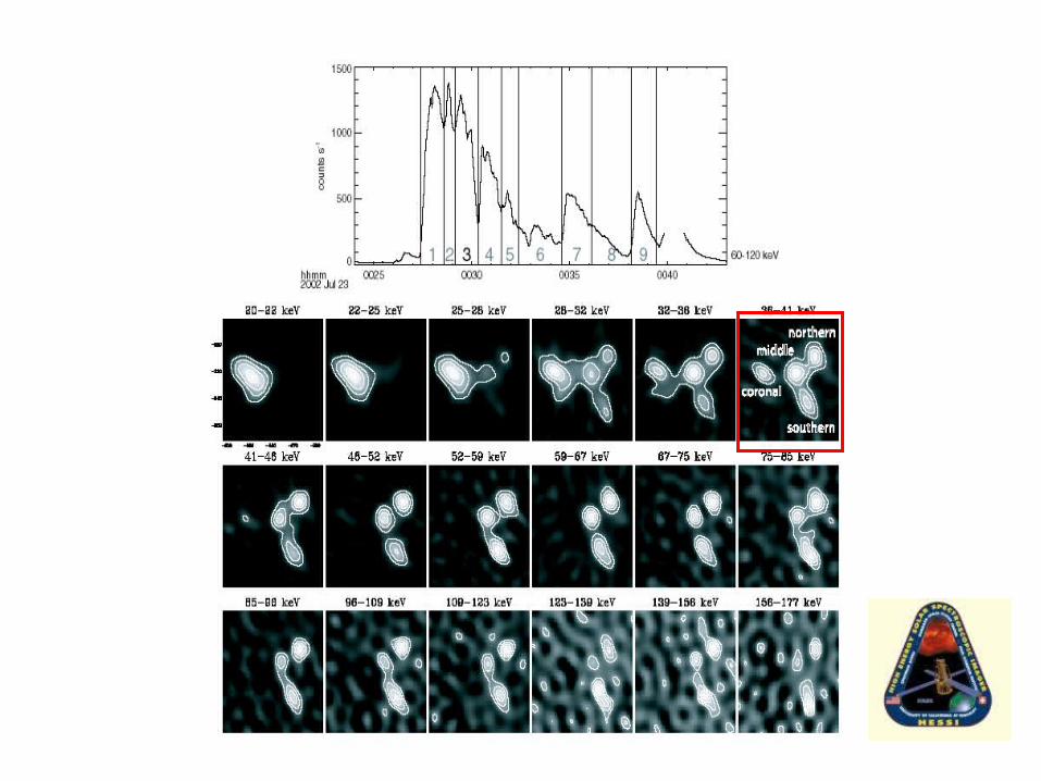

Feature Spectra
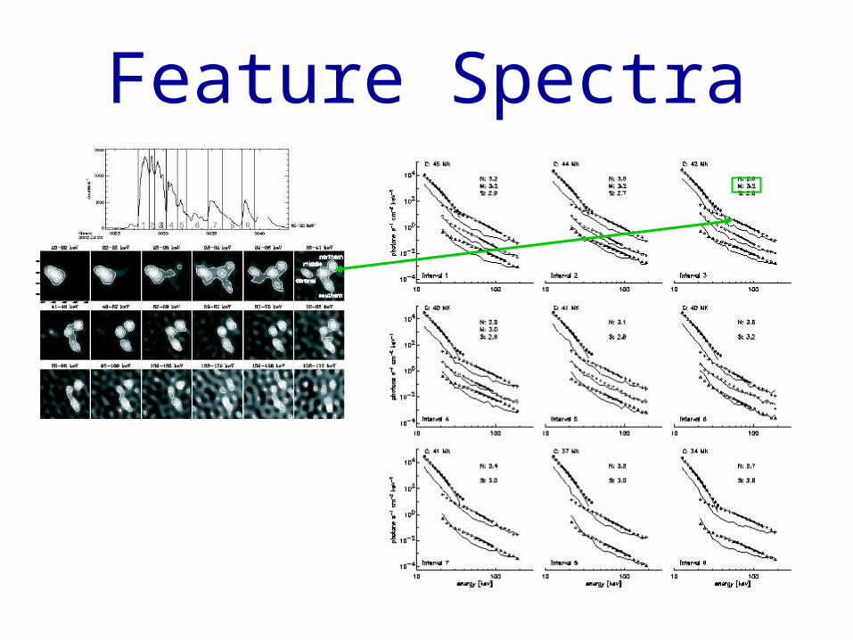
Feature Spectra

Feature Spectra

Feature Spectra

Temporal Trends
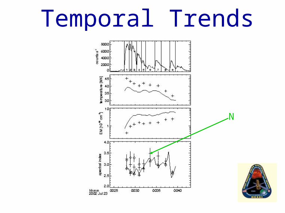
Temporal Trends
N
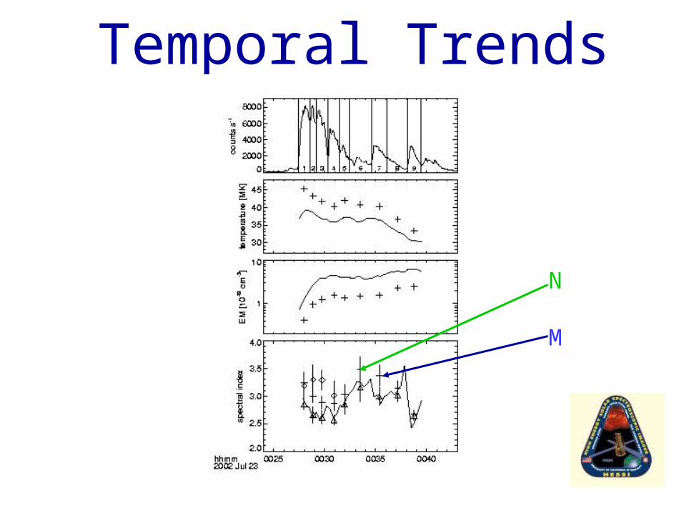
Temporal Trends
N
M
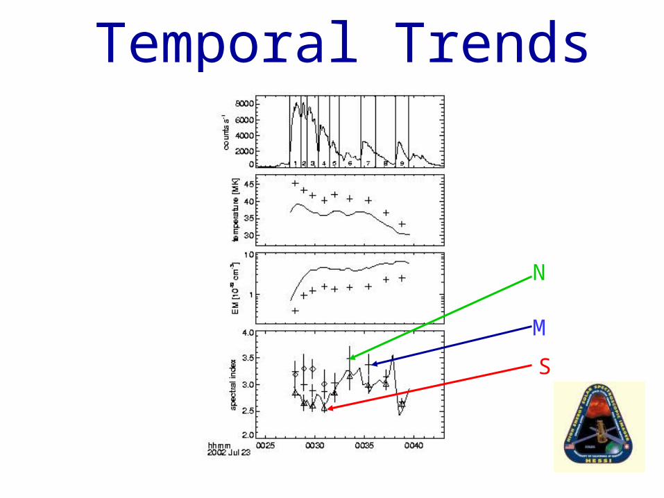
Temporal Trends
N
M
S

Implications for Particle Transport
• Spectrum at one footpoint (South) consistently harder
• This is consistent with collisional transport through a greater mass of material!

Atmospheric Response
• Collisional heating temperature rise
• Temperature rise pressure increase
• Pressure increase mass motion
• Mass motion density changes
• “Evaporation”
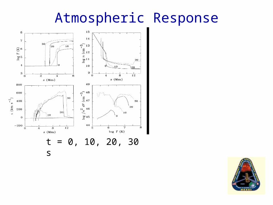
Atmospheric Response
t = 0, 10, 20, 30 s
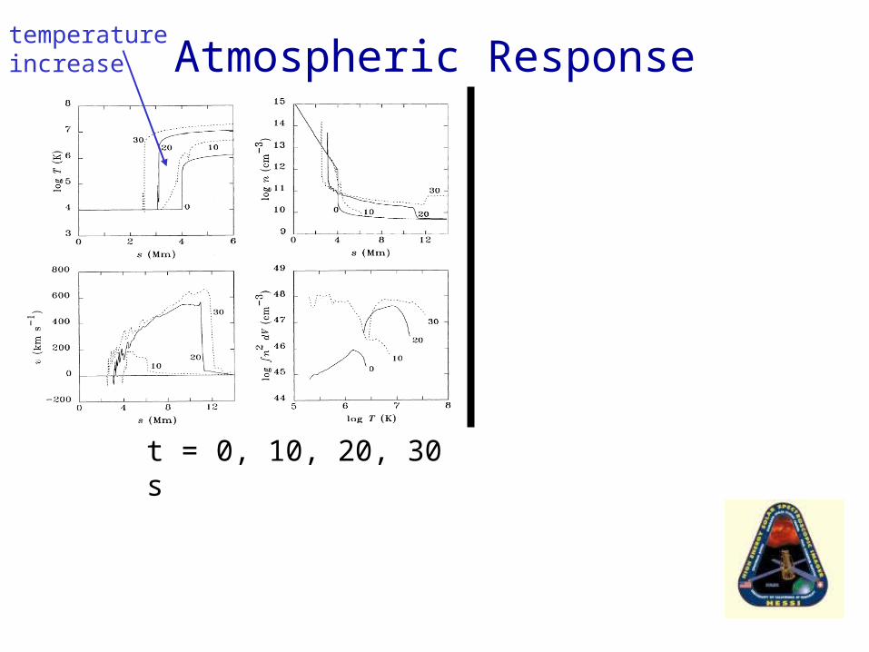
Atmospheric Response
t = 0, 10, 20, 30 s
temperature increase

Atmospheric Response
t = 0, 10, 20, 30 s
upward motion
temperature increase

Atmospheric Response
t = 0, 10, 20, 30 s
upward motion
temperature increase
increased density

Atmospheric Response
t = 0, 10, 20, 30 s t = 40, 50, 60 s
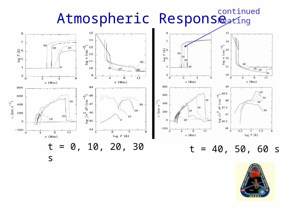
Atmospheric Response
t = 0, 10, 20, 30 s t = 40, 50, 60 s
continued heating

Atmospheric Response
t = 0, 10, 20, 30 s t = 40, 50, 60 s
continued heating
subsiding motions

Atmospheric Response
t = 0, 10, 20, 30 s t = 40, 50, 60 s
continued heating
subsiding motions
enhanced soft X-ray emission

The “Neupert Effect”
• Hard X-ray (and microwave) emission proportional to injection rate of particles (“power”)
• Soft X-ray emission proportional to accumulated mass of high-temperature plasma (“energy”)
• So, we expect
ISXR ~ IHXR dt

Inference of transport processes from observations
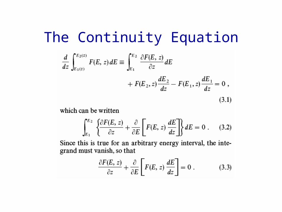
The Continuity Equation

Using Spatially Resolved Hard X-ray Data to Infer Physical Processes
• Electron continuity equation: F(E,N)/ N + / E [F(E,N) dE/dNdE/dN] = 0
• Solve for dE/dN:dE/dNdE/dN = - [1 / F(E,N)] [ F(E,N)/ N] dE
• So observation of F(E,N) gives direct empirical information on physical processes (dE/dNdE/dN) at work

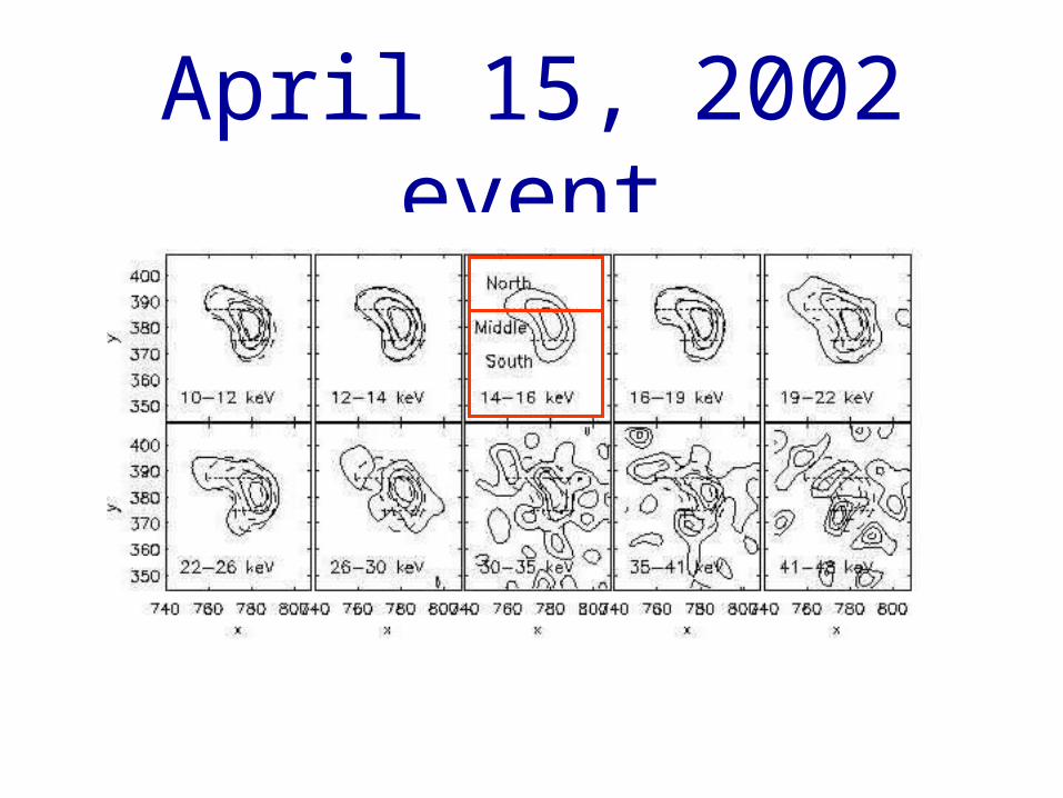
April 15, 2002 event

April 15, 2002 event
April 15, 2002 event

April 15, 2002 event
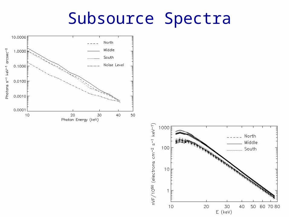
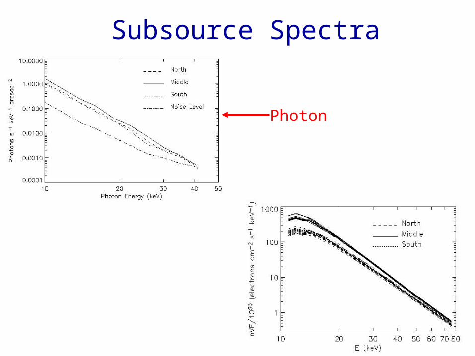
Subsource Spectra
Subsource Spectra
Photon

Subsource Spectra
Photon
Electron

Subsource Spectra
Photon
Electron
‘Middle’ region spectrum is softer

Subsource Spectra
Photon
Electron
‘Middle’ region spectrum is softer
Spectrum reminiscent of collisional variation

Subsource Spectra
Photon
Electron
‘Middle’ region spectrum is softer
Spectrum reminiscent of collisional variation
But
dE/dN= -[1/F(E,N)] [ F(E,N)/ N] dE ?

Variation of Source Size with Energy• Collisions: dE/ds ~ -n/E L ~ 2
In general, L increases with (increased penetration of higher energy electrons)
• General: dE/ds ~ -n/E L ~ 1+
• Thermal: T ~ To exp(-s2/22) L(,To,)
In general, L decreases with (highest-energy emission near temperature peak)

26 – 30 keV
19 - 22 keV
14 - 16 keV
10 - 12 keV
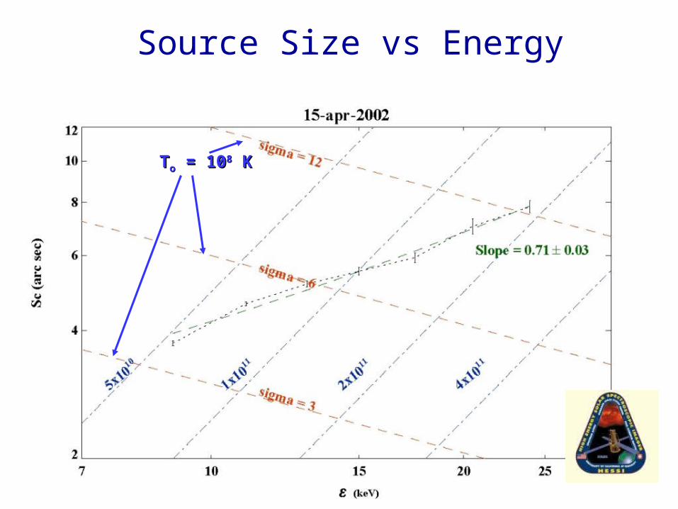
Source Size vs Energy
TToo = 10 = 1088 K K

Histogram of Slopes
NOT compatible with slope of 2!NOT compatible with slope of 2!
Significance of Observed Slope
• Collisions
dE/ds ~ - n/E, =1, slope = 1 + = 2
Significance of Observed Slope
• Collisions
dE/ds ~ - n/E, =1, slope = 1 + = 2
• Observed mean slope 1 + ~ 0.5

Significance of Observed Slope
• Collisions
dE/ds ~ - n/E, =1, slope = 1 + = 2
• Observed mean slope 1 + ~ 0.5
~ -0.5

Significance of Observed Slope
• Collisions
dE/ds ~ - n/E, =1, slope = 1 + = 2
• Observed mean slope 1 + ~ 0.5
~ -0.5
dE/ds ~ - nE0.5 ~ -nv (??)