mathematics

Article

Particle Swarm Optimization for Predicting theDevelopment Effort of Software Projects

Mariana Dayanara Alanis-Tamez 1,2, Cuauhtémoc López-Martín 3,* andYenny Villuendas-Rey 4,*

1 Centro de Investigación en Computación, Instituto Politécnico Nacional, Juan de Dios Bátiz s/n,Nueva Industrial Vallejo, GAM, CDMX, Mexico City 07700, Mexico; b160626@sagitario.cic.ipn.mx

2 Oracle, Fusion Adaptative Intelligence, Paseo Valle Real 1275, Valle Real, Zapopan, Jal,Guadalajara 45136, Mexico

3 Department of Information Systems, Universidad de Guadalajara, Periférico Norte N 799,Núcleo Universitario Los Belenes, Zapopan 45100, Jalisco, Mexico

4 Centro de Innovación y Desarrollo Tecnológico en Cómputo, Instituto Politécnico Nacional,Juan de Dios Bátiz s/n, Nueva Industrial Vallejo, GAM, CDMX, Mexico City 07700, Mexico

* Correspondence: yvilluendasr@ipn.mx (C.L.-M.); cuauhtemoc@cucea.udg.mx (Y.V.-R.)

Received: 22 September 2020; Accepted: 14 October 2020; Published: 17 October 2020

Abstract: Software project planning includes as one of its main activities software development effortprediction (SDEP). Effort (measured in person-hours) is useful to budget and bidding the projects.It corresponds to one of the variables most predicted, actually, hundreds of studies on SDEP havebeen published. Therefore, we propose the application of the Particle Swarm Optimization (PSO)metaheuristic for optimizing the parameters of statistical regression equations (SRE) applied to SDEP.Our proposal incorporates two elements in PSO: the selection of the SDEP model, and the automaticadjustment of its parameters. The prediction accuracy of the SRE optimized through PSO (PSO-SRE)was compared to that of a SRE model. These models were trained and tested using eight data sets ofnew and enhancement software projects obtained from an international public repository of projects.Results based on statistically significance showed that the PSO-SRE was better than the SRE in six datasets at 99% of confidence, in one data set at 95%, and statistically equal than SRE in the remaining dataset. We can conclude that the PSO can be used for optimizing SDEP equations taking into account thetype of development, development platform, and programming language type of the projects.

Keywords: software project planning; software development effort prediction; particle swarmoptimization; ISBSG

1. Introduction

Software engineering management involves planning [1]. The software project planning includessoftware prediction, and the most common predicted variables have been size [2] (mainly measuredin either source lines of code, or function points [3]), effort (in person-hours or person-months [3]),duration (in months [4]), and quality (in defects [5]).

Software development effort prediction (SDEP), also termed effort estimation or cost estimation [6],is needed for managers to estimate the monetary cost of projects. As reference, in USA the cost byperson-month (which is equivalent to 152 person-hours) is of $8000 USD [7].

Unfortunately, those projects taking more time (i.e., time overrun) costing more money (i.e., costoverrun) [8], and cost overrun has been identified as a chronic problem in most software projects [9];whereas for cost underrun, a portion of the budgeted money is not spent and then money taxes haveto be paid. These issues related to costs have been the causes for which a software project has beenassessed based upon the ability to achieve the budgeted cost [10,11].

Mathematics 2020, 8, 1819; doi:10.3390/math8101819 www.mdpi.com/journal/mathematics

Mathematics 2020, 8, 1819 2 of 21

The relevance of the SDEP has been reflected with several publications on systematic reviewspublished between the years 2007 [6] and 2020 [12] where hundreds of studies on SDEP had beenanalyzed. The prediction models identified in the systematic reviews have been adaptive ridgeregression, association rules, Bayesian networks, case-based reasoning (CBR, also termed analogy-based),decision trees, expectation maximization, fuzzy logic, genetic programming, grey relational analysis,neural networks, principal component analysis, random forest, and support vector regressions.

The proposal of accurate models for SDEP represents a continuous activity of researchers andsoftware managers. On average, software developers spend between 30% and 40% more effort than ispredicted when planning any project. The failure attributed to SDEP leads to schedule delays and costoverruns, which can address project failure and affect the reputation and competitiveness. On the otherhand, over-predicting the effort of a software project can address ineffective use of resources, whichcan result in loss of opportunities to fund other projects, and therefore loss of tenders. It can derive,from a social point of view, demotivation of software engineers and their probable search for new jobopportunities. These scenarios have motivated researchers for addressing their efforts to determinewhich prediction technique is most accurate, or to propose new or combined techniques that couldprovide better predictions [13].

There are several kinds of techniques, which have been applied to SDEP of projects developedindividually in academic settings [14] or by teams of practitioners [12]. Our study involves projectsdeveloped by teams of practitioners in business environments.

As for metaheuristic algorithms, several studies on them have recently been published betweenthe years 2019 and 2020 being inspired from (a) social behavior of animals, that is, Particle SwarmOptimization (PSO) such as insects, herds, birds and fishes [15], bats [16], butterflies [17], cuckoos [18],elephants [19], fireflies [20], moths [21], and whales [16]; (b) nature (brain [22], differential evolution [16],and genetic algorithm (GA) [23]), (c) physics (cooling of metals [24]), and (d) mathematics (such as sineand cosine operators [24]).

Regarding software engineering field, metaheuristics have also been specifically applied for SDEP.The applied algorithms have been artificial bee colony (ABC) [25], cuckoo search [26], differentialevolution [27], GA [28], PSO [29], simulated annealing [30], tabu search [30], and whale optimizationalgorithm [31].

In those ten studies that we identified where PSO was applied to SDEP (which are analyzed in theSection 2 of the present study), PSO has been used to optimize parameters of models such as Bayesianbelief network [32], CBR [33–37], COCOMO statistical equation [38] (whose model was publishedin the year of 1981 [39]), decision trees [40], fuzzy logic [29], mathematical expressions [25], neuralnetworks [40], and support vector regression [40].

Regarding those five studies where PSO is used for optimizing CBR, in four of them the mostsimilar software projects are selected, and the effort of a new project is predicted through a weightedaverage obtained from data of those similar projects. These weights are calculated using PSO [34–37].In the fifth study, the authors use a hybrid CBR using local and global searches, and a multi-objectivePSO is used to minimize two error functions for the searching [33]. As for fuzzy logic, the PSO isused to optimize the parameter values of the membership functions that make up the model [29]. In adifferent manner, once a set of fuzzy models has been defined, PSO is used to choose that model thatbest fits the SDEP [38]. PSO has also been used in combination with elements from ABC algorithmto fit the parameters of a predefined SDEP function [25]. Other study uses a classifier committee tomake predictions and uses PSO to optimize the parameter values of each of the base classifiers thatmake up that classifier committee [40]. In a similar perspective, PSO was used within a hybrid model,to estimate the components of a Bayesian network [32]. In our proposal, neither weights nor any CBRmodel to be optimized are considered.

Unlike the previous proposals, the contribution of our study is the application of the PSO algorithmto optimize the parameters of statistical regression equations (SRE) applied to SDEP (hereafter, termedPSO-SRE), the selection of which is also optimized. Each equation is generated by following a

Mathematics 2020, 8, 1819 3 of 21

regression analysis, and from data sets of projects selected from an international public repository ofrecent software projects (i.e., International Software Benchmarking Standards Group, ISBSG release2018). The software projects were selected based on their type of development (TD), developmentplatform (DP), and programming language type (PLT) as suggested in the guidelines of the ISBSG [41].The ISBSG has widely been used for SDEP models [42].

The size of a software project is a common variable used for SDEP [3], therefore, our models use itas the independent variable. In our study, the size type is function points, whose value is calculatedfrom nineteen independent variables mentioned in the Section 4 of the present study (i.e., adjustedfunction points, AFP) [13].

The justification for the comparison between the prediction accuracy of our PSO-SRE with thatobtained from SRE is based on the following issues related to SDEP:

(a) The prediction accuracy of any new proposed model should at least outperform a SRE [43].(b) SRE has been the model whose prediction accuracy has mostly been compared to other models

such as those based on ML [44,45].(c) The prediction accuracy of SRE has outperformed the accuracies obtained from ML models [44].

Owing to a statistical analysis is needed for a validity studies [46], the data preprocessing andour conclusions are based on statistical analysis involving identification of outliers, coefficients ofcorrelation and determination of data, as well as on the suitable statistical test for comparing theprediction accuracy between PSO-SRE and SRE.

A systematic literature review published in 2018 which analyzed studies published between 1981and 2016 on SDEP models recommends the use of same data sets and a same prediction accuracymeasure such that conclusions can be compared to other studies [3]. This recommendation wassuggested once they found difficulty to compare the performance among SDEP models due to thewide diversity of data sets and accuracy measures used. Thus, in our study, the models were appliedto the same data sets, as well as taking into account a same accuracy measure (i.e., absolute residual,AR). Moreover, they were trained and tested using the same validation method (i.e., a Leave-one-outcross-validation, LOOOV, which is recommended for software effort model evaluation [47]).

In the present study, the null (H0) and alternative (H1) hypotheses to be tested are the following:

H0. Prediction accuracy of the PSO-SRE is statistically equal to that of the SRE when these two models areapplied to predict the development effort of software projects using the AFP as the independent variable.

H1. Prediction accuracy of the PSO-SRE is statistically not equal to that of the SRE when these two models areapplied to predict the development effort of software projects using the AFP as the independent variable.

The remaining of the present study is as follows: Section 2 has been assigned to describe the relatedstudies where PSO has been applied to predict the development effort of software projects. Section 3describes the Particle Swarm Optimization (PSO) metaheuristic, and our proposal: the PSO-SRE.Section 4 presents the criteria applied to select the data sets of software projects by observing theguidelines of the ISBSG, as well as the data preprocessing. Section 5 presents the results when PSO-SREis performed and compares its prediction accuracy to SRE once the two models were trained andtested. Section 6 mentions our conclusions. Finally, Section 7 corresponds to a discussion section,which includes the comparison with previous studies, the limitations of our study, validation threats,as well as directions for future work.

2. Related Work

The proposed SDEP techniques have been systematically analyzed in severalreviews [3,6,12,44,45,48–51]. They can be classified in those not based on models, and in thosebased on models. The first type mentioned is also termed expert judgment [48,52], whereas the latterone can be classified in two categories: statistical [53] and ML models [44,45].

Mathematics 2020, 8, 1819 4 of 21

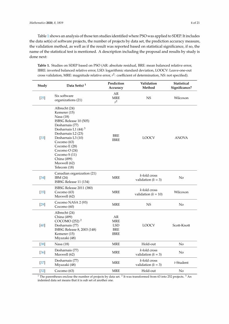
Table 1 shows an analysis of those ten studies identified where PSO was applied to SDEP. It includesthe data set(s) of software projects, the number of projects by data set, the prediction accuracy measure,the validation method, as well as if the result was reported based on statistical significance, if so, thename of the statistical test is mentioned. A description including the proposal and results by study isdone next:

Table 1. Studies on SDEP based on PSO (AR: absolute residual, BRE: mean balanced relative error,IBRE: inverted balanced relative error, LSD: logarithmic standard deviation, LOOCV: Leave-one-outcross validation, MRE: magnitude relative error, r2: coefficient of determination, NS: not specified).

Study Data Set(s) 1 PredictionAccuracy

ValidationMethod

StatisticalSignificance?

[25] Six softwareorganizations (21)

ARMRE

r2NS Wilcoxon

[33]

Albrecht (24)Kemerer (15)Nasa (18)ISBSG Release 10 (505)Desharnais (77)Desharnais L1 (44) 3

Desharnais L2 (23)Desharnais L3 (10)Cocomo (63)Cocomo E (28)Cocomo O (24)Cocomo S (11)China (499)Maxwell (62)Telecom (18)

BREIBRE LOOCV ANOVA

[34]Canadian organization (21)IBM (24)ISBSG Release 11 (134)

MRE k-fold crossvalidation (k = 3) No

[35]ISBSG Release 2011 (380)Cocomo (63)Maxwell (62)

MRE k-fold crossvalidation (k = 10) Wilcoxon

[29] Cocomo NASA 2 (93)Cocomo (60) MRE NS No

[40]

Albrecht (24)China (499)COCOMO (252) 2

Desharnais (77)ISBSG Release 8, 2003 (148)Kemerer (15)Miyazaki (48)

ARMRELSDBREIBRE

LOOCV Scott-Knott

[38] Nasa (18) MRE Hold-out No

[36] Desharnais (77)Maxwell (62) MRE k-fold cross

validation (k = 3) No

[37] Desharnais (77)Miyazaki (48) MRE k-fold cross

validation (k = 3) t-Student

[32] Cocomo (63) MRE Hold-out No1 The parentheses enclose the number of projects by data set. 2 It was transformed from 63 into 252 projects. 3 Anindented data set means that it is sub set of another one.

Mathematics 2020, 8, 1819 5 of 21

Azzeh et al. [33] use PSO to find the optimum solutions for variables related to multiple evaluationmeasures when applied CBR. Their results show that CBR improves when taking into account allvariables together.

Bardsiri et al. [34] apply PSO to optimize the CBR weights. The PSO algorithm assigns weights tothe features considered in the similarity function. The accuracy of their proposal is compared to thoseobtained from three types of CBR, as well as to those ones obtained from neural networks, classificationand regression tree, and statistical regression models. Results show that the prediction accuracy of theCBR when used PSO was better than all the mentioned models.

Bardsiri et al. [35] use PSO in combination with CBR to design a weighting system in which theproject attributes of different clusters of software projects are given different weights. The performanceof their proposal is better than the prediction accuracy obtained when neural networks, classificationand regression trees, and statistical regression models are applied.

Chhabra and Singh [29] firstly compare the prediction accuracy of three models termedRegression-Based COCOMO, Fuzzy COCOMO, and PSO Optimized Fuzzy COCOMO. In the latterone, they use the PSO to optimize the fuzzy logic model parameters. Then, they also compare theperformance of it to that of a GA Optimized Fuzzy COCOMO. Their results show that the PSOOptimized Fuzzy COCOMO has better prediction accuracy than those obtained from the other threemodels. They concluded that the PSO can be applied as optimizer for a fuzzy logic model.

Hosni et al. [40] apply PSO for setting ensemble parameters of four ML models. They comparethe PSO performance to that of grid search. They conclude that PSO and grid search show a samepredictive capability when applied to k-nearest neighbor, support vector regression, neural networks,and decision trees.

Khuat and Le [25] propose an algorithm combining the PSO and ABC algorithms for optimizingthe parameters of a SDEP formula. This formula is generated by using two independent variablesobtained from agile software projects (i.e., final velocity, and story point). The accuracy results byapplying this formula are compared to those obtained from four types of neural networks (i.e., generalregression neural network, probabilistic neural network, group method of data handling polynomialneural network, and cascade correlation neural network). The performance of the algorithm based onPSO and ABC was better than those obtained from the four mentioned neural networks.

Sheta et al. [38] use PSO for optimizing the parameters of the COCOMO equation (termedPSO-COCOMO). They also build a fuzzy system. The PSO-COCOMO has a better performance thanthose obtained when the SDEP equations proposed by Halstead, Walston-Felix, Bailey-Basili, and Dotyare applied.

Wu et al. [36] use PSO to optimize the CBR weights. They employ Euclidean, Manhattan,and grey relational grade distances as metrics to calculate the similarity measures. Their resultsshow that the weighed CBR generates better prediction accuracy than unweighted CBR methods.They concude that the combined method integrating PSO and CBR improves the performance for thethree mentioned measures.

Wu et al. [37] use PSO in combination with six CBR methods. These methods differ by their typeof distance measure (i.e., Euclidean, Manhattan, Minkowski, grey relational coefficient, Gaussian,and Mahalanobis). Results show that the combination of methods proposed by them has a betterperformance than independent methods, and that the weighted mean combination method has abetter result.

Zare et al. [32] apply PSO to obtain the optimal updating coefficient of effort prediction basedon the concept of optimal control by modifying the predicted value of a Bayesian belief network.Its performance is compared to that obtained when applied GA. Results of their proposed model indicatethat optimal updating coefficient obtained by GA increases the accuracy of prediction significantly incomparison with that obtained from PSO.

In accordance with Table 1, only two studies used a non-biased prediction accuracy measure(i.e., AR), only two of them used a deterministic validation method (i.e., LOOCV), the half of them based

Mathematics 2020, 8, 1819 6 of 21

their conclusions on statistically significance, and none of the them involved any recent repositoryof software projects: Albrecht was published in the year of 1983, Canadian organization in 1996,COCOMO in 1981, Desharnais in 1988, IBM in 1994, Kemerer in 1987, Maxwell in 1993, Miyazaki in1994, Nasa in 1981, Telecom in 1997, and the most recent ISBSG release used was published in the yearof 2011. Regarding the data set of projects of the six software organizations, it was published in 2012;however, its size is small: 21 projects [25]. Finally, the year of those projects of China was not reportedin those studies that have used them [33,40].

In those four studies where the ISBSG data set was used, the releases were 8 [40], 10 [33] and11 [34,35], whose years of publication and sizes were 2003 with 2000 software projects, 2007 with 4000,and 2009 with 5052, respectively. When the release 8 was used, the authors selected a data set of 148projects based on the following ISBSG criteria: DT (new), quality rating (“A” and “B” categories),resource level with 1 as value, maximum number of people working on the project, number of businessunits, and IFPUG as functional sizing method (FSM) type [40]. As for release 10, they selected a data setof 505 projects taking into account only a criterion suggested by the ISBSG: the quality rating (“A”) [33].As for release 11: (a) they selected a data set of 134 projects based on three ISBSG criteria: quality rating(“A” and “B”), normalized effort ratio of up to 1.2, and “Insurance” value for the type of organizationattribute [34], and (b) they selected a data set of 380 projects based on quality rating attribute (“A” and“B”), DT, organization type, DP, normalized effort ratio of up to 1.2, resource level with 1 as value,and IFPUG as FSM [35]. That is, in all of these four studies, only one data set was selected by study,and the type of FSM was not taken into account to select the data set by mixing the IFPUG versions.

In accordance with the analysis of these ten studies, PSO has been used in three fundamentalmanners: (a) as a tool to support CBR [33–37,40], (b) for the selection of the SDEP model [38], and (c) forthe optimization of values of a SDEP model ([25,29,32]). In our opinion, the manner in how PSO wasused in these studies has the following disadvantages:

(a) An increase in the computational cost inherent to CBR models by incorporating the use ofoptimization techniques.

(b) Allowing selecting the best SDEP model from a set of predefined models, but without anautomatically adjustment of the parameters of the selected model.

(c) Define a priori the SDEP model to be used, and only adjusting its parameters.

Taking into account these weaknesses, our proposal incorporates the following two elementsin PSO:

(1) The selection of the SDEP model, and(2) The automatic adjustment of the SDEP model parameters.

The analysis of the Table 1 also allows us emphasizing our experimental design which involvesnew and enhancement software projects selected based on their TD, DP, PLT, and FSM. Data of theseprojects are preprocessed through an outlier analysis, and calculation of two types of coefficients:correlation and determination. The models are trained and tested based on AR while a LOOCV isapplied. Finally, the hypotheses of our study are statistically tested.

3. Particle Swarm Optimization (PSO) and PSO-SRE

3.1. PSO

Particle Swarm Optimization (PSO) is an optimization model created in 1995 by Kennedy andEberhart [54]. It assumes that there is a cloud of particles, which “fly” in a D dimensional space.This original idea was refined three years later considering the introduction of memory into particles [55].Particles have access to two types of memory: individual memory (the best position occupied bythe particle in space) and collective memory (the best position occupied by the cloud in space).The evolution of the original PSO has continuously been analyzed [15].

Mathematics 2020, 8, 1819 7 of 21

In PSO, the size of the particle cloud np (number of particles) is considered as a user parameter.In the cloud, each particle i has stored the following three real vectors of D dimensions: the currentposition vector xi, the vector of the best position reached pi, and the flight speed vector vi. In addition,the cloud or swarm stores the best global position vector gbest.

The movement of the particles is defined as a change in their position, when adjusting a velocityvector, component by component. To do this, the particles use individual memory and collectivememory. The j-th component of the velocity vector of the i-th particle is updated as:

vi, j ← w ∗ vi, j + c1 ∗ rand(0, 1) ∗(pi j − xi, j

)+ c2 ∗ rand(0, 1) ∗

(gbest, j − xi, j

)(1)

where w is the inertia weight, c1 is the individual memory coefficient, and c2 is the global memorycoefficient. The function rand(0, 1) represents the generation of a random number in the [0, 1] interval.If the velocity components exceed the established limits, they are bounded, such that it complied thatVmin ≤ vi, j ≤ Vmax.

Subsequently, the j-th component of the current position vector of the i-th particle is adjusted as:

xi, j ← xi, j + vi, j (2)

This adjusting process on the positions for the particles is repeated until a stop condition isachieved, which is usually settled as a number of algorithm iterations.

The pseudocode of the PSO algorithm described by Shi and Eberhart [55] is shown in Figure 1.It assumes that it is intended to minimize an objective function.

Mathematics 2020, 8, 1819 7 of 21

particle in space) and collective memory (the best position occupied by the cloud in space). The evolution of the original PSO has continuously been analyzed [15].

In PSO, the size of the particle cloud np (number of particles) is considered as a user parameter. In the cloud, each particle 𝑖 has stored the following three real vectors of D dimensions: the current position vector 𝑥 , the vector of the best position reached 𝑝 , and the flight speed vector 𝑣 . In addition, the cloud or swarm stores the best global position vector 𝑔 .

The movement of the particles is defined as a change in their position, when adjusting a velocity vector, component by component. To do this, the particles use individual memory and collective memory. The j-th component of the velocity vector of the i-th particle is updated as: 𝑣 , ← 𝑤 ∗ 𝑣 , + 𝑐 ∗ 𝑟𝑎𝑛𝑑(0,1) ∗ 𝑝 − 𝑥 , + 𝑐 ∗ 𝑟𝑎𝑛𝑑(0,1) ∗ 𝑔 , − 𝑥 , (1)

where 𝑤 is the inertia weight, 𝑐 is the individual memory coefficient, and 𝑐 is the global memory coefficient. The function 𝑟𝑎𝑛𝑑(0,1) represents the generation of a random number in the [0, 1] interval. If the velocity components exceed the established limits, they are bounded, such that it complied that 𝑉 ≤ 𝑣 , ≤ 𝑉 .

Subsequently, the j-th component of the current position vector of the i-th particle is adjusted as: 𝑥 , ← 𝑥 , + 𝑣 , (2)

This adjusting process on the positions for the particles is repeated until a stop condition is achieved, which is usually settled as a number of algorithm iterations.

The pseudocode of the PSO algorithm described by Shi and Eberhart [55] is shown in Figure 1. It assumes that it is intended to minimize an objective function.

Figure 1. Pseudocode of the PSO algorithm. Figure 1. Pseudocode of the PSO algorithm.

Mathematics 2020, 8, 1819 8 of 21

In terms of complexity and time execution, PSO has two external loops that are generation loopsand a loop through the entire population. In each loop, the optimization function is computed for eachmember of the population (particle). Considering k as the cost of computing the optimization function,it can be said that the time of execution of PSO is bounded by O(it ∗ np ∗ k).

3.2. PSO-SRE

We use a PSO design considering an additional element: the SDEP model. Thus, the 20 functionsdetailed in Table 2 were taken into account to achieve it. The x independent variable used in these20 functions corresponds to the FSM (i.e., AFP). We add an additional component to each individual,which corresponds to an integer number in the interval [1,20] which represents the SDEP model to beused by the particle. Consequently, each particle has a different number of dimensions, which will varyaccording to the coefficients of the selected model. This novel modification allows us to simultaneouslyoptimize the SDEP model to be selected, as well as its parameters. Figure 2 shows a swarm of fiveparticles used by our proposed algorithm. The pseudocode of the proposal is shown in Figure 3.

Table 2. Description of the analyzed models.

No. Model Equation Reference

1 Linear equation y = a + bx [56]2 Exponential equation y = aekx [56]3 Exponential decrease or increase between limits y = aebx + c [57]4 Double exponential decay to zero y = ae−bx + ce−dx [57]5 Power y = axb [57]6 Asymptotic equation y = a + b

x [58]7 Asymptotic regression model y = a− (a− b)e−cx [56]8 Logarithmic y = alnx + b [57]9 “Plateau” curve—Michaelis-Menten equation y = ax

b+x [57]10 Yield-loss/density curves y = iX

1+ iXa

[54]

11 Logistic Function y = 11+e−ax [57]

12 Logistic curves with additional parameters y = bc+e−ax [57]

13 Logistic curve with offset on the y-Axis y = 11+eb+cx + d [57]

14 Gaussian curve y =exp[−(x−µ)2/2σ2]

σ√

2π[57]

15 Log vs. Reciprocal y =(a− b

x

)[57]

16 Trigonometric functions y = a sin(bx + c) + d [57]17 Trigonometric functions (2) y = sin ax + sin bx [57]

18 Trigonometric functions (3) y = a sin(bx + c) +d sin(ex + f ) + g [57]

19 Quadratic polynomial regression y = a + bx + cx2 [57]20 Cubic polynomial regression y = a + bx + cx2 + dx3 [57]

Mathematics 2020, 8, 1819 8 of 21

In terms of complexity and time execution, PSO has two external loops that are generation loops and a loop through the entire population. In each loop, the optimization function is computed for each member of the population (particle). Considering 𝑘 as the cost of computing the optimization function, it can be said that the time of execution of PSO is bounded by 𝑂(𝑖𝑡 ∗ 𝑛𝑝 ∗ 𝑘). 3.2. PSO-SRE

We use a PSO design considering an additional element: the SDEP model. Thus, the 20 functions detailed in Table 2 were taken into account to achieve it. The x independent variable used in these 20 functions corresponds to the FSM (i.e., AFP). We add an additional component to each individual, which corresponds to an integer number in the interval [1,20] which represents the SDEP model to be used by the particle. Consequently, each particle has a different number of dimensions, which will vary according to the coefficients of the selected model. This novel modification allows us to simultaneously optimize the SDEP model to be selected, as well as its parameters. Figure 2 shows a swarm of five particles used by our proposed algorithm. The pseudocode of the proposal is shown in Figure 3.

Figure 2. Swarm of five particles, using the proposed codification. The first component denotes the model number, as in Table 2, and the remaining ones the parameters to optimize of the selected model.

Figure 3. Pseudocode of the modified PSO algorithm.

Figure 2. Swarm of five particles, using the proposed codification. The first component denotes themodel number, as in Table 2, and the remaining ones the parameters to optimize of the selected model.

Mathematics 2020, 8, 1819 9 of 21

Mathematics 2020, 8, 1819 8 of 21

In terms of complexity and time execution, PSO has two external loops that are generation loops and a loop through the entire population. In each loop, the optimization function is computed for each member of the population (particle). Considering 𝑘 as the cost of computing the optimization function, it can be said that the time of execution of PSO is bounded by 𝑂(𝑖𝑡 ∗ 𝑛𝑝 ∗ 𝑘). 3.2. PSO-SRE

We use a PSO design considering an additional element: the SDEP model. Thus, the 20 functions detailed in Table 2 were taken into account to achieve it. The x independent variable used in these 20 functions corresponds to the FSM (i.e., AFP). We add an additional component to each individual, which corresponds to an integer number in the interval [1,20] which represents the SDEP model to be used by the particle. Consequently, each particle has a different number of dimensions, which will vary according to the coefficients of the selected model. This novel modification allows us to simultaneously optimize the SDEP model to be selected, as well as its parameters. Figure 2 shows a swarm of five particles used by our proposed algorithm. The pseudocode of the proposal is shown in Figure 3.

Figure 2. Swarm of five particles, using the proposed codification. The first component denotes the model number, as in Table 2, and the remaining ones the parameters to optimize of the selected model.

Figure 3. Pseudocode of the modified PSO algorithm. Figure 3. Pseudocode of the modified PSO algorithm.

Based on Figure 2, it can be defined that to obtain the final value to be compared for each particle,the first value is taken, which is the one that corresponds to the number of the model shown in Table 2,together with the following n values that correspond to the model parameters. As example, for theparticle [1, 0.24, 0.18], the first value (1) would correspond to model 1 of the Table 2 and the nexttwo values (0.24, 0.18) correspond to the parameters a and b to optimize the selected model, which is:y = a + bx obtained by the SDEP model.

We use the first dimension to determine the equation assigned to the particle. By this, we use adynamic codification, and the particles will have different dimensions, depending on the assignedequation. The dimensions of the particles range from two to five.

To update the velocity vector of a particle, if the value of gbest has more dimensions, the ones thatare needed are used, and if it has fewer dimensions, we use random numbers instead. The particleshave in common that they use mathematical equations to optimize the prediction of the effort ofsoftware projects. A particle interacts with itself (updating its best position) and with the best particleof the swarm. Even if a particle and the best particle have different equations, using the coefficients ofthe best particle helps the particle to move towards a global optimum. If we use random guessing,we do not consider the fitness results. On the other hand, if we use the best particle, we considerthe fitness.

We consider that using the proposed codification offers the proposed PSO-SRE more searchspace capacity (exploration) and allows it to get better out of local optimums. However, for otheroptimizations problems, this increase in the search capacity of the proposal can be prone to not givingthe best results, due to the decrease in the exploitation capacity of the proposal.

The dimension and model will be unique for each data set and, once the stop condition is attained,the test MAR value will be calculated.

Mathematics 2020, 8, 1819 10 of 21

A crucial aspect of optimization algorithms such as PSO lies in the selection of the optimizationfunction. In our research, two optimization functions (i.e., the prediction accuracy measures) areevaluated: AR, and the MAR. AR is calculated by ith-project as follows [13]:

ARi = |Actual Efforti − Predicted Efforti| (3)

And the mean of ARs as follows:

MAR = (1/N)∑

ARi (4)

The median of ARs is denoted by MdAR. The accuracy of a prediction model is inverselyproportional to the MAR or MdAR.

The parameter values for the proposed PSO model are: w = 0.1, Vmin = −10, Vmax = 10 andc1 = c2 = 1.5, this last value was chosen due to it had better results in our experiments, comparedto that recommended as a standard value (i.e., c1 = c2 = 2 [54]). The swarm size was evaluatedconsidering np between 50 and 750, whereas the iteration number was set between 250 and 1500.

As optimization function, we use the MAR of the training set, considering a LOOCV for thecorresponding model defined in Table 2.

4. Data Sets of Software Projects

In the present study, the data sets used were obtained from the ISBSG release 2018, which is aninternational public repository whose data of software projects developed between 1989 and 2016, werereported from 32 countries. Among these countries are Spain, United States, Netherlands, Finland,France, Australia, India, Japan, Canada, and Denmark [59]. The projects were selected observingthe ISBSG guidelines by selecting the data sets taking into account the quality of data, FSM, TD,DP, and PLT [41]. Table 3 describes the number of projects by applying each criterion (the ISBSGclassifies the quality data of projects from “A” to “D” types, and “A” and “B” are recommended forstatistical analysis). Since IFPUG V4 projects with V4 and post V4 should not be mixed [41], only thoseprojects whose FSM corresponded to IFPUG 4+ were selected. In classifying the final 2054 projects ofTable 3 by DT, 618 of them were new, 1416 enhanced and 20 re-development projects. The types of DPreported by the ISBSG are mainframe (MF), midrange (MR), multiplatform (Multi), personal computer(PC), and proprietary, whereas the PLT are second (2GL), third (3GL), fourth (4GL) generation, andapplication generator (ApG). As for the resource level, the ISBSG classifies it in accordance with howeffort is quantified, and the level 1 corresponds to development team effort [41]. Those new andenhancement data sets were selected since they are the larger ones.

Table 3. Criteria for selecting the data sets from the ISBSG (8261 projects).

Attribute Selected Value(s) Projects

Adjusted Function Point not null — 6394Data quality rating A, B 6061Unadjusted Function Point Rating A, B 5316Functional sizing methods IFPUG 4+ 4602Development platform not null — 3040Language type not null — 2711Resource level 1 2054

The IFPUGV4+ FSM is reported in AFP, which is a composite value calculated from the followingnineteen variables: internal logical file, external interface files, external inputs, external outputs, externalinquiries, data communications, distributed data processing, performance, heavily used configuration,transaction rate, on-line data entry, end-user efficiency, on-line update, complex processing, reusability,installation ease, operational ease, multiple sites, and facilitate change [13].

Mathematics 2020, 8, 1819 11 of 21

Table 4 classifies those final 2034 new and enhancement projects classified in accordance withcriteria included in Table 3. Since the χ2 statistical normality test to be applied in this study needs atleast thirty data, a scatter plot (Effort vs. AFP) was generated by data set whose number of projects inTable 4 was higher or equal than thirty (i.e., fifteen data sets). The scatter plots of these fifteen data setsfrom the Table 4 showed skewness, heteroscedasticity, and presence of outliers, therefore, in Table 5four statistical normality tests are applied for Effort and AFP variables. Table 5 shows that there isat least a p-value lower than 0.01 by data set. It means that can be rejected the idea that Effort andAFP come from a normal distribution with 99% confidence for all of the data sets. Therefore, data arenormalized applying them the natural logarithm (ln), which ensures that the resulting model goesthrough the origin on the raw data scale [43]. As example, Figures 4 and 5 depict those scatter plotscorresponding to that data set of Table 4 having 133 new software projects. Figures 4 and 5 depict theraw and transformed data, respectively.

Table 4. Projects classified by type of development (TD), development platform (DP), and programminglanguage type (PLT), NSP: Number of software projects.

TD DP PLT NSP

New MF 2GL 3MF 3GL 133MF 4GL 28MF ApG 4MR 3GL 36MR 4GL 22

Multi 3GL 105Multi 4GL 102

PC 3GL 55PC 4GL 118

Proprietary 5GL 12Enhancement MF 2GL 4

MF 3GL 457MF 4GL 48MF ApG 53MR 3GL 67MR 4GL 53

Multi 3GL 442Multi 4GL 195

PC 3GL 55PC 4GL 42

Table 5. Normal statistical tests by data set (NSP: number of software projects; S-W: Shapiro-Wilk).

TD DP PLT NSP VariableNormality Test

χ2 S-W Skewness Kurtosis

New MF 3GL 133 AFP 0.0000 0.0000 0.0000 0.0000Effort 0.0000 0.0000 0.0000 0.0000

MR 3GL 36 AFP 0.0354 0.0075 0.1836 0.8342Effort 0.0000 0.0000 0.0000 0.0000

Multi 3GL 105 AFP 0.0000 0.0000 0.0000 0.0000Effort 0.0000 0.0000 0.0000 0.0000

Multi 4GL 102 AFP 0.0000 0.0000 0.0000 0.0000Effort 0.0000 0.0000 0.0000 0.0000

PC 3GL 55 AFP 0.0000 0.0000 0.0000 0.0000Effort 0.0000 0.0000 0.0000 0.0000

PC 4GL 118 AFP 0.0000 0.0000 0.0002 0.0158Effort 0.0000 0.0000 0.0000 0.0000

Mathematics 2020, 8, 1819 12 of 21

Table 5. Cont.

TD DP PLT NSP VariableNormality Test

χ2 S-W Skewness Kurtosis

Enhancement MF 3GL 457 AFP 0.0000 0.0000 0.0000 0.0000Effort 0.0000 0.0000 0.0000 0.0000

MF 4GL 48 AFP 0.0000 0.0000 0.0000 0.0000Effort 0.0186 0.0000 0.0104 0.0300

MF ApG 53 AFP 0.0000 0.0000 0.0000 0.0000Effort 0.0000 0.0000 0.0002 0.0000

MR 3GL 67 AFP 0.0000 0.0000 0.0000 0.0000Effort 0.0000 0.0000 0.0000 0.0000

MR 4GL 53 AFP 0.0000 0.0000 0.0117 0.1535Effort 0.0000 0.0000 0.0001 0.0000

Multi 3GL 442 AFP 0.0000 0.0000 0.0000 0.0000Effort 0.0000 0.0000 0.0000 0.0000

Multi 4GL 195 AFP 0.0000 0.0000 0.0000 0.0000Effort 0.0000 0.0000 0.0000 0.0000

PC 3GL 55 AFP 0.0000 0.0000 0.0003 0.0003Effort 0.0000 0.0000 0.0000 0.0000

PC 4GL 42 AFP 0.0000 0.0000 0.0006 0.0001Effort 0.0203 0.0000 0.0047 0.0006

Mathematics 2020, 8, 1819 12 of 21

MF 4GL 48 AFP 0.0000 0.0000 0.0000 0.0000 Effort 0.0186 0.0000 0.0104 0.0300 MF ApG 53 AFP 0.0000 0.0000 0.0000 0.0000 Effort 0.0000 0.0000 0.0002 0.0000 MR 3GL 67 AFP 0.0000 0.0000 0.0000 0.0000 Effort 0.0000 0.0000 0.0000 0.0000 MR 4GL 53 AFP 0.0000 0.0000 0.0117 0.1535 Effort 0.0000 0.0000 0.0001 0.0000 Multi 3GL 442 AFP 0.0000 0.0000 0.0000 0.0000 Effort 0.0000 0.0000 0.0000 0.0000 Multi 4GL 195 AFP 0.0000 0.0000 0.0000 0.0000 Effort 0.0000 0.0000 0.0000 0.0000 PC 3GL 55 AFP 0.0000 0.0000 0.0003 0.0003 Effort 0.0000 0.0000 0.0000 0.0000 PC 4GL 42 AFP 0.0000 0.0000 0.0006 0.0001 Effort 0.0203 0.0000 0.0047 0.0006

Figure 4. Raw data of 133 software projects.

Figure 5. Transformed data of Figure 4.

Outliers were identified based on studentized residuals greater than 2.5 in absolute value. The outliers, as well as coefficients of correlation (r) and determination (r2) by data set are included in Table 6. In accordance with the number of acceptable outliers, a 5% of them by data set was taken as reference [60]. As for a minimum percentage for the coefficient of determination, at least a r2 value higher than 0.5 was considered since it has been accepted for SDEP models [61]. Thus, in this study, eight data sets of those fifteen analyzed in Table 6 were selected to generate their corresponding PSO-SRE and SRE. They were finally selected since three of the fifteen had a r2 value lower than 0.5, three of them presented a percentage between 11% and 16.6% of outliers, and one of them had a r2 = 0.4119 with 14.28% of outliers.

Figure 4. Raw data of 133 software projects.

Mathematics 2020, 8, 1819 12 of 21

MF 4GL 48 AFP 0.0000 0.0000 0.0000 0.0000 Effort 0.0186 0.0000 0.0104 0.0300 MF ApG 53 AFP 0.0000 0.0000 0.0000 0.0000 Effort 0.0000 0.0000 0.0002 0.0000 MR 3GL 67 AFP 0.0000 0.0000 0.0000 0.0000 Effort 0.0000 0.0000 0.0000 0.0000 MR 4GL 53 AFP 0.0000 0.0000 0.0117 0.1535 Effort 0.0000 0.0000 0.0001 0.0000 Multi 3GL 442 AFP 0.0000 0.0000 0.0000 0.0000 Effort 0.0000 0.0000 0.0000 0.0000 Multi 4GL 195 AFP 0.0000 0.0000 0.0000 0.0000 Effort 0.0000 0.0000 0.0000 0.0000 PC 3GL 55 AFP 0.0000 0.0000 0.0003 0.0003 Effort 0.0000 0.0000 0.0000 0.0000 PC 4GL 42 AFP 0.0000 0.0000 0.0006 0.0001 Effort 0.0203 0.0000 0.0047 0.0006

Figure 4. Raw data of 133 software projects.

Figure 5. Transformed data of Figure 4.

Outliers were identified based on studentized residuals greater than 2.5 in absolute value. The outliers, as well as coefficients of correlation (r) and determination (r2) by data set are included in Table 6. In accordance with the number of acceptable outliers, a 5% of them by data set was taken as reference [60]. As for a minimum percentage for the coefficient of determination, at least a r2 value higher than 0.5 was considered since it has been accepted for SDEP models [61]. Thus, in this study, eight data sets of those fifteen analyzed in Table 6 were selected to generate their corresponding PSO-SRE and SRE. They were finally selected since three of the fifteen had a r2 value lower than 0.5, three of them presented a percentage between 11% and 16.6% of outliers, and one of them had a r2 = 0.4119 with 14.28% of outliers.

Figure 5. Transformed data of Figure 4.

Outliers were identified based on studentized residuals greater than 2.5 in absolute value.The outliers, as well as coefficients of correlation (r) and determination (r2) by data set are included inTable 6. In accordance with the number of acceptable outliers, a 5% of them by data set was taken asreference [60]. As for a minimum percentage for the coefficient of determination, at least a r2 valuehigher than 0.5 was considered since it has been accepted for SDEP models [61]. Thus, in this study,eight data sets of those fifteen analyzed in Table 6 were selected to generate their correspondingPSO-SRE and SRE. They were finally selected since three of the fifteen had a r2 value lower than 0.5,

Mathematics 2020, 8, 1819 13 of 21

three of them presented a percentage between 11% and 16.6% of outliers, and one of them had ar2 = 0.4119 with 14.28% of outliers.

Table 6. Normalized data sets of software projects (NSP: number of software projects, NO: number ofoutliers, FDSS: final data set size).

TD DP LT NSP NO FDSS % r r2

New MF 3GL 133 3 130 2.25 0.7345 0.5396MR 3GL 36 6 30 16.6 0.7390 0.5461

Multi 3GL 105 6 99 5.71 0.7227 0.5223Multi 4GL 102 6 96 5.88 0.8513 0.7247

PC 3GL 55 7 48 12.72 0.7978 0.6365PC 4GL 118 6 112 5.08 0.6515 0.4245

Enhancement MF 3GL 457 17 440 3.86 0.7916 0.6266MF 4GL 48 4 44 9.09 0.4751 0.2257MF ApG 53 4 49 8.16 0.6571 0.4318MR 3GL 67 3 64 4.68 0.8052 0.6483MR 4GL 53 6 47 11.32 0.7127 0.5080

Multi 3GL 442 14 428 3.16 0.8016 0.6427Multi 4GL 195 5 190 2.56 0.7640 0.5838

PC 3GL 55 2 53 3.77 0.8019 0.6431PC 4GL 42 6 36 14.28 0.6418 0.4119

The model for the SRE is linear having the form ln(Effort) = a + b * ln(AFP). Table 7 contains theSRE by data set selected from Table 6. All equations coincide with the assumption of developmenteffort: the higher size (i.e., AFP), the higher effort is.

Table 7. SREs for predicting the effort of new and enhancement projects.

TD DP LT SRE

New MF 3GL ln(E f f ort) = 4.28 + 0.72 ∗ ln(AFP)Multi 3GL ln(E f f ort) = 3.90 + 0.73 ∗ ln(AFP)Multi 4GL ln(E f f ort) = 1.69 + 0.99 ∗ ln(AFP)

Enhancement MF 3GL ln(E f f ort) = 3.53 + 0.83 ∗ ln(AFP)MR 3GL ln(E f f ort) = 4.03 + 0.67 ∗ ln(AFP)

Multi 3GL ln(E f f ort) = 2.13 + 1.08 ∗ ln(AFP)Multi 4GL ln(E f f ort) = 3.79 + 0.70 ∗ ln(AFP)

PC 3GL ln(E f f ort) = 2.84 + 0.82 ∗ ln(AFP)

5. Results

A total of 130, 99, 96, 440, 64, 428, 190 and 53 SREs were generated by data set once a LOOCVwas performed.

The proposed PSO-SRE algorithm was executed for each dataset with different configurations in adistributed manner and on a dedicated server for the laboratory, trying to ensure that the executiontime was as short as possible and trying to get the best possible result.

After applying the PSO-SRE, it is possible to detail the selected SDEP model (from those onesincluded in Table 2) by data set. Table 8 includes the PSO-SRE configuration in terms of the number ofiterations, as well as the swarm size for three types of tests described next (the values were selectedfrom those configurations described in the previous paragraph):

1. Test 1: Up to 500 iterations, and up to 250 individuals in the swarm;2. Test 2: Up to 1500 iterations, and up to 750 individuals in the swarm;3. Test 3: Up to 1000 iterations, and up to 500 individuals in the swarm.

Mathematics 2020, 8, 1819 14 of 21

Table 8. PSO parameters by data set (TD: type of development, DP: development platform LT:programming language, NSP: number of software projects, ID-SRE: unique identifier of the generatedSRE) for the Tests (SS: Swarm size, DEDZ: Double exponential decay to zero, LE: Linear equation, Pcu:“Plateau” curve, AE: Asymptotic equation).

TD DP LT NSP IDSRE

ModelName

Test 1 Test 2 Test 3

SS Iterations SS Iterations SS Iterations

NewMF 3GL 130 1 DEDZ 50 250 150 750 100 500

Multi 3GL 99 2 LE 50 250 150 750 100 500Multi 4GL 96 3 LE 50 250 150 750 100 500

Enhancement MF 3GL 440 4 LE 250 500 750 1500 500 1000MR 3GL 64 5 LE 50 250 150 750 100 500

Multi 3GL 428 6 Pcu 50 250 150 750 100 500Multi 4GL 190 7 Pcu 50 250 150 750 100 500

PC 3GL 53 8 AE 50 500 150 1500 100 1000

As for velocity updates, Barrera et al. [62] address the issue of defining velocity limits iteratively.They show that for some optimization functions, the velocity update reported by Shi and Eberhart [55], issusceptible to sub-optimal behavior. However, for predicting the effort of software projects, we obtainedgood results with the approach of Shi and Eberhart [55].

The number of iterations and swarm size depend on the data set converging in different conditions.In relating the swarm size and iteration number of the three different tests of Table 8 to the predictionaccuracy of Table 9 by data set, we can conclude that the increase of swarm size and iteration numberdegrades the performance of the proposed PSO-SRE algorithm. In accordance with Test 1 data, we canconclude that between 250 and 500 iterations, and a swarm size between 50 and 250 correspond tovalues which can be suggested for generate better results.

Table 9. Prediction accuracies by model.

TD IDSRE

LT NSPSRE RS

PSO-SRE

Test 1 Test 2 Test 3

MAR MdAR MAR MdAR MAR MdAR MAR MdAR MAR MdAR

New1 3GL 130 0.66 0.60 1.73 1.83 0.54 0.41 0.61 0.51 0.61 0.512 3GL 99 0.62 0.56 1.46 1.35 0.56 0.43 0.61 0.55 0.61 0.553 4GL 96 0.53 0.49 0.74 0.57 0.43 0.32 0.52 0.47 0.52 0.47

Enhancement

4 3GL 440 0.61 0.52 1.99 2.01 0.61 0.50 0.61 0.50 0.61 0.525 3GL 64 0.60 0.50 1.33 1.21 0.53 0.35 0.59 0.49 0.59 0.496 3GL 428 0.56 0.50 1.62 1.60 0.40 0.28 0.55 0.48 0.54 0.467 4GL 190 0.52 0.44 1.37 1.46 0.46 0.41 0.51 0.45 0.51 0.458 3GL 53 0.72 0.70 1.18 1.06 0.48 0.36 0.72 0.70 0.65 0.55

Table 9 includes the prediction accuracy obtained by model. It shows that PSO-SRE had a betterMAR than SRE in seven of the eight data sets, and equal than the remaining one for Test 1, that is,when swarm size and number of iterations were lower than those of Test 2 and Test 3. In addition,the MARs for the Test 1 data sets were better than those MARs of Test 2 and Test 3 for all data setsexcept for one data set in which the MAR resulted equal for the three Tests (MAR = 0.61). Thus, dataobtained from Test 1 are used in the present study.

In Table 9, we include a simple Random Search (RS) algorithm, which:

• not have memory of its own nor a search direction,• repeat the random search of “the best particle” for a number of times that is equal to the number

of fitness evaluations in the proposed PSO-SRE,• compare its best solution with the best solution yielded by PSO-SRE.

Since a MAR is not sufficient to report results in studies on software effort prediction, a suitablestatistical test is applied for comparing the accuracies of the two models [46]. The selection of this test

Mathematics 2020, 8, 1819 15 of 21

should be based in the number of data sets to be compared, data dependence and data distribution.In our study, two data sets will be compared at a time, and they are dependent (because each modelwas applied to each project by data set). As for data distribution, firstly, a new data set is obtainedby each of the eight data sets of Table 9. Each new data set is obtained from the difference betweenthe two ARs by project (an AR of SRE, and an AR of PSO-SRE). Secondly, four normality statisticaltests are performed to each new data set. Thirdly, if any of their four p-values is lower than 0.05 or0.01, then data are non-normally distributed at 95% or 99% of confidence, respectively, and a Wilcoxontest should be applied (the medians of models should be compared to accept/reject the hypothesis),otherwise, a t-paired should be performed (the means of models should then be compared) [63].Table 10 shows that only in two cases the data resulted normally distributed, then, in the restingfourteen cases, a Wilcoxon test was applied, and the medians were used for the fourteen comparisons.

Table 10. Statistical tests for data distribution and between models by data set. PSO: (PSO-SRE – SRE),RS: (PSO-SRE – RS).

TD DP LT NSP Pair χ2 S-W Skewness Kurtosis p-Value

New

MF 3GL 130 SRE 0.0000 0.0000 0.3410 0.0000 0.0000RS 0.0000 0.0000 0.0073 0.9537 0.0000

Multi 3GL 99 SRE 0.0000 0.0000 0.0000 0.0000 0.0040RS 0.1462 0.0160 0.2573 0.6616 0.0000

Multi 4GL 96 SRE 0.0000 0.0000 0.2251 0.0000 0.0000RS 0.2261 0.0387 0.8034 0.0428 0.0000

Enhancement

MF 3GL 440 SRE 0.0000 0.0000 0.6019 0.0000 0.3878RS 0.0000 0.0000 0.0000 0.0014 0.0000

MR 3GL 64 SRE 0.0016 0.5511 0.7769 0.9573 0.0267RS 0.7847 0.8470 0.6219 0.9685 0.0000

Multi 3GL 428 SRE 0.0000 0.0000 0.1028 0.0000 0.0000RS 0.0000 0.0000 0.0000 0.5221 0.0000

Multi 4GL 190 SRE 0.0000 0.0000 0.8475 0.0000 0.0000RS 0.0002 0.0000 0.0322 0.1907 0.0000

PC 3GL 53 SRE 0.0347 0.0002 0.0961 0.0155 0.0000RS 0.8419 0.2107 0.5087 0.3184 0.0000

An important issue regarding PSO-SRE is the computational complexity. The server used forperforming the tests had the following characteristics: OS: Ubuntu 20.04.1 LTS x86_64, Host: PowerEdgeR720, Kernel: 5.4.0-47-generic, CPU: Intel Xeon E5-2620 0 <24> @2.500 GHz, GPU: NVIDIA TeslaK20Xm, GPU: NVIDIA GeForce 210 and Memory: 4828 MiB/64,347 MiB.

We executed the algorithm in a distributed manner (i.e., datasets in parallel), which reduced theexecution time. However, we made a sequential set of experiments (i.e., one dataset at the time) toestimate the total time expended in each set of experiments considering the LOOCV used. Table 11shows the time (sequential) by data set. Its column “Prediction” refers to the time of using the proposedPSO-SRE to predict the effort of a software project for each of the datasets. As shown in Table 11,the proposed PSO-SRE is able to predict the effort of a software project in less than half a minute.

Mathematics 2020, 8, 1819 16 of 21

Table 11. Execution time of the experiments, using a sequential approach.

TD DP LT NSP Model NameExecution Time (Minutes)

Test 1 Test 2 Test 3 Prediction

New MF 3GL 130 Double ExponentialDecay to Zero 14.5 23.6 36.1 0.28

Multi 3GL 99 Linear equation 10.8 19.1 30.0 0.30Multi 4GL 96 Linear equation 10.7 18.9 28.9 0.30

Enhancement MF 3GL 440 Linear equation 61.6 122.2 183.6 0.42MR 3GL 64 Linear equation 7.1 14.4 17.9 0.28

Multi 3GL 428 “Plateau” curve 49.8 103.8 165.1 0.39Multi 4GL 190 “Plateau” curve 18.9 27.9 49.8 0.26

PC 3GL 53 Asymptotic equation 5.3 9.2 15.1 0.28

6. Conclusions

The results showed in the Tables 9 and 10 allow us accepting the following alternative hypothesisformulated in the Section 1 of our study in favor of PSO-SRE for seven of the eight data sets (six ofthem at 99% of confidence, and the seventh one at 95% of confidence):

Prediction accuracy of the PSO-SRE is statistically not equal to that of the SRE when thesetwo models are applied to predict the development effort of software projects using the AFP as theindependent variable.

Regarding the remaining data set, the following null hypothesis is accepted at 99% of confidence:Prediction accuracy of the PSO-SRE is statistically equal to that of the SRE when these two

models are applied to predict the development effort of software projects using the AFP as theindependent variable.

As for the comparison between the PSO-SRE and RS, the following hypothesis can be accepted infavor of the PSO-SRE for the eight data sets at 99% of confidence:

Prediction accuracy of the PSO-SRE is statistically not equal to that of the RS when these twomodels are applied to predict the development effort of software projects using the AFP as theindependent variable.

We can conclude that a software manager can apply PSO-SRE for predicting the developmenteffort of a software project taking into account the following TD, DP, and PLT when AFP is used as theindependent variable:

(a) New software projects coded in 3GL and developed in either Mainframe or Multiplatform andcoded in 4GL and developed in Multiplatform.

(b) Software enhancement projects coded in 3GL and developed in Multiplatform, MidRange orpersonal computer, as well as in those projects coded in 4GL and developed in Multiplatform.

(c) Since the performance of the PSO-SRE resulted statistically equal than SRE, a software managercould also apply PSO-SRE as alternative to an SRE to software enhancement projects coded in3GL and developed in Mainframe.

Regarding PSO-SRE optimization, from a general perspective, the best prediction accuracy bydata set was obtained when the number of iterations was between 250 and 500, and the swarm sizebetween 50 and 250.

7. Discussion

In software prediction, one of the most common predicted software variables has been effort,which is commonly measured in person-hours or person-month. SDEP is needed for managers toestimate the cost of projects and then for budgeting and bidding; actually, its importance can be showedin the hundreds of studies published in the last forty years. Thus, in the present study, the PSO wasapplied for optimizing the parameters of SDEP equations. The prediction accuracy of the PSO-SRE

Mathematics 2020, 8, 1819 17 of 21

was compared to that obtained from SRE. Both types of models were generated based on eight datasets of software projects selected by observing the guidelines of the ISBSG.

In comparing our study with those ten identified ones where PSO has been applied to SDEP anddescribed in Table 1, we identify the following issues:

• None of them generate their models by using a recent repository of software projects.• Regarding the four studies where the ISBSG is used (1) their releases correspond to those published

in the years 2007 and 2009, (2) all of them only select one data set from the ISBSG whose sizes arebetween 134 and 505, and (3) none of them take into account the version of the FSM to select thedata set; whereas in our study, (1) the ISBSG release 2018 was used, (2) eight data sets containingbetween 53 and 440 projects were selected, and (3) all of them took into account the guidelinessuggested by the ISBSG, including the type of FSM, that is, our data sets did not mix IFPUG V4type with V4 and post V4 one.

• The majority of them base their conclusions on a biased prediction accuracy measure, and on anondeterministic validation method.

• The half of them bases their conclusions on statistically significance.

We did not find any study having all of the following characteristics as ours when proposedthe PSO-SRE:

(1) The use of PSO incorporating an additional component by allowing automatic completion, in asingle step, of the selection of the SDEP model, and automatic adjustment of the parameters ofthe SDEP model.

(2) New and enhancement software projects obtained from the ISBSG release 2018.(3) Software projects selected taking into account the TD, DP, PLT, and FSM as suggested by the ISBSG.(4) Preprocessing of data sets through outliers’ analysis, and correlation and

determination coefficients.(5) A nonbiased prediction accuracy measure (i.e., AR) to compare the performance between PSO-SRE

and SRE models.(6) The use of a deterministic validation method for training and testing the models (i.e., LOOCV)(7) Selection of a suitable statistical test based on number of data sets to be compared, data dependence,

and data distribution for comparing the prediction accuracy between PSO-SRE and SRE by data set.(8) Hypotheses tested from statistically significance.

Our manuscript also followed all of the six guidelines when a new SDEP model is proposed [43] by(1) confirming that our PSO-SRE algorithm outperforms a statistical model (i.e., SRE), when PSO-SREoutperformed to SRE in seven of the eight data sets with statistical significance, (2) taking into accountthe heteroscedasticity, skewness, and heterogeneity of effort and size data of software projects, (3) usingstatistical tests to compare the performance between prediction models, (4) explaining in detail howour PSO-SRE is applied, (5) justifying the selection of any statistical test we used, and (6) including thecriteria followed for selecting the data sets of software projects from the ISBSG.

A first limitation of the present study that reduces the generalization of our conclusions is relatedto the number of data sets used, that is, in spite of the ISBSG contains more than eight thousands ofsoftware projects, we could only select eight data sets observing the guidelines of the ISBSG. A secondone is that only 20 prediction models are considered based on simple SRE (Table 2). Finally, a thirdlimitation is that we did not consider other more complex ML prediction models.

As for external threat validity, the prediction accuracy of PSO-SRE will depend on an accurateestimation performed by the practitioner on the independent variable value (i.e., the size measuredin AFP).

Another limitation regarding the use of heuristic algorithms (PSO in this paper) is that they prunethe search space and can discard useful regions. We are aware that the proposed method, despite its

Mathematics 2020, 8, 1819 18 of 21

good behavior for predicting the effort of software projects, can have a different performance for otheroptimization problems.

Future work will be related to the application of other metaheuristics for optimizing the parametersfor the SRE. We will intent to use a greater number of datasets, whose data is current and reflecting theheterogenic evolution of these data. Alternative models will also be proposed to predict the effort ofnew and enhancement software projects such as those based on classifiers [64,65]. Moreover, additionalprediction accuracy measure criteria will be take account such as standardized accuracy and effectsize [66]. Finally, a modification to the algorithm can be added to take duplicate values into accountand to act similarly between them, as well as to apply alternative update mechanisms as in [62] for thevelocity update, and test it against the one currently used. We will also explore newer and improvedimplementations of PSO.

Author Contributions: Conceptualization, C.L.-M. and Y.V.-R.; methodology, C.L.-M., M.D.A.-T. and Y.V.-R.;software, M.D.A.-T. and Y.V.-R.; validation, C.L.-M. and Y.V.-R.; formal analysis, M.D.A.-T. and Y.V.-R.; investigation,C.L.-M., M.D.A.-T. and Y.V.-R.; writing—original draft preparation, C.L.-M. and Y.V.-R.; writing—review andediting, M.D.A.-T. and Y.V.-R.; visualization, C.L.-M. and Y.V.-R. All authors have read and agreed to the publishedversion of the manuscript.

Funding: This research received no external funding.

Acknowledgments: The authors would like to thank the Centro de Innovación y Desarrollo Tecnológico enCómputo and the Centro de Investigación en Computación, both of the Instituto Politécnico Nacional, México;Universidad de Guadalajara, México, and the Consejo Nacional de Ciencia y Tecnología (CONACyT), México.

Conflicts of Interest: The authors declare no conflict of interest.

Abbreviations

The following abbreviations are used in this manuscript:

2GL Programming languages of second generation3GL Programming languages of third generation4GL Programming languages of fourth generationABC Artificial bee colonyAFP Adjusted function pointsApG Application generatorAR Absolute residualCBR Case-based reasoningCOCOMO Constructive cost modelDP Development platformFSM Functional sizing methodGA Genetic algorithmIFPUG International Function Point Users GroupISBSG International Software Benchmarking Standards GroupLOOCV Leave one-out cross validationMAR Mean absolute residualsMdAR Median of absolute residualsMF MainframeML Machine learningMR MidrangeMulti MultiplatformPC Personal computerPLT Programming language typePSO Particle swarm optimizationPSO-SRE SRE optimized by means of PSOSDEP Software development effort predictionSRE Statistical regression equationTD Type of development

Mathematics 2020, 8, 1819 19 of 21

References

1. Bourque, P.; Fairley, R. Guide to the Software Engineering Body of Knowledge, SWEBOK V3.0; IEEE ComputerSociety: Washington, DC, USA, 2014.

2. Wilkie, F.G.; McChesney, I.R.; Morrowa, P.; Tuxworth, C.; Lester, N.G. The value of software sizing. Inf. Softw.Technol. 2011, 53, 1236–1249. [CrossRef]

3. Gautam, S.S.; Singh, V. The state-of-the-art in software development effort estimation. J. Softw. Evol. Process2018, 30, e1983. [CrossRef]

4. Pospieszny, P.; Czarnacka-Chrobot, B.; Kobylinski, A. An effective approach for software project effort andduration estimation with machine learning algorithms. J. Syst. Softw. 2018, 137, 184–196. [CrossRef]

5. Li, Z.; Jing, X.-Y.; Zhu, X. Progress on approaches to software defect prediction. IET Softw. 2018, 12, 161–175.[CrossRef]

6. Jorgensen, M.; Shepperd, M. A Systematic Review of Software Development Cost Estimation Studies.IEEE Trans. Softw. Eng. 2007, 33, 33–53. [CrossRef]

7. Boehm, B.; Abts, C.; Brown, A.W.; Chulani, S.; Clark, B.K.; Horowitz, E.; Madachy, R.; Reifer, D.J.; Steece, B.Software Cost Estimation with COCOMO II; Prentice Hall: Upper Saddle River, NY, USA, 2000.

8. Ahsan, K.; Gunawan, I. Analysis of cost and schedule performance of international development projects.Int. J. Proj. Manag. 2010, 28, 68–78. [CrossRef]

9. Doloi, H.K. Understanding stakeholders’ perspective of cost estimation in project management. Int. J.Proj. Manag. 2011, 29, 622–636. [CrossRef]

10. Jørgensen, M. The effects of the format of software project bidding processes. Int. J. Proj. Manag. 2006, 24,522–528. [CrossRef]

11. Savolainen, P.; Ahonen, J.J.; Richardson, I. Software development project success and failure from thesupplier’s perspective: A systematic literature review. Int. J. Proj. Manag. 2012, 30, 458–469. [CrossRef]

12. Carbonera, C.E.; Farias, K.; Bischoff, V. Software development effort estimation: A systematic mapping study.IET Softw. 2020, 14, 328–344. [CrossRef]

13. López-Martín, C. Predictive Accuracy Comparison between Neural Networks and Statistical Regression forDevelopment Effort of Software Projects. Appl. Soft Comput. 2015, 27, 434–449. [CrossRef]

14. Chavoya, A.; López-Martín, C.; Andalon-Garcia, I.R.; Meda-Campaña, M.E. Genetic programming asalternative for predicting development effort of individual software projects. PLoS ONE 2012, 7, e50531.[CrossRef] [PubMed]

15. Wang, D.; Tan, D.; Liu, L. Particle swarm optimization algorithm: An overview. Soft Comput. 2018, 22,387–408. [CrossRef]

16. Yeoh, J.M.; Caraffini, F.; Homapour, E.; Santucci, V.; Milani, A. A Clustering System for Dynamic DataStreams Based on Metaheuristic Optimisation. Mathematics 2019, 7, 1229. [CrossRef]

17. Kim, M.; Chae, J. Monarch Butterfly Optimization for Facility Layout Design Based on a Single Loop MaterialHandling Path. Mathematics 2019, 7, 154. [CrossRef]

18. García, J.; Yepes, V.; Martí, J.V. A Hybrid k-Means Cuckoo Search Algorithm Applied to the CounterfortRetaining Walls Problem. Mathematics 2020, 8, 555. [CrossRef]

19. Li, J.; Guo, L.; Li, Y.; Liu, C. Enhancing Elephant Herding Optimization with Novel Individual UpdatingStrategies for Large-Scale Optimization Problems. Mathematics 2019, 7, 395. [CrossRef]

20. Balande, U.; Shrimankar, D. SRIFA: Stochastic Ranking with Improved-Firefly-Algorithm for ConstrainedOptimization Engineering Design Problems. Mathematics 2019, 7, 250. [CrossRef]

21. Feng, Y.; An, H.; Gao, X. The Importance of Transfer Function in Solving Set-Union Knapsack Problem Basedon Discrete Moth Search Algorithm. Mathematics 2019, 7, 17. [CrossRef]

22. Shih, P.-C.; Chiu, C.-Y.; Chou, C.-H. Using Dynamic Adjusting NGHS-ANN for Predicting the RecidivismRate of Commuted Prisoners. Mathematics 2019, 7, 1187. [CrossRef]

23. Grigoras, , G.; Neagu, B.-C.; Gavrilas, , M.; Tris, tiu, I.; Bulac, C. Optimal Phase Load Balancing in Low VoltageDistribution Networks Using a Smart Meter Data-Based Algorithm. Mathematics 2020, 8, 549. [CrossRef]

24. Jouhari, H.; Lei, D.; A. A. Al-qaness, M.; Abd Elaziz, M.; Ewees, A.A.; Farouk, O. Sine-Cosine Algorithm toEnhance Simulated Annealing for Unrelated Parallel Machine Scheduling with Setup Times. Mathematics2019, 7, 1120. [CrossRef]

Mathematics 2020, 8, 1819 20 of 21

25. Khuat, T.T.; Le, M.H. A Novel Hybrid ABC-PSO Algorithm for Effort Estimation of Software Projects UsingAgile Methodologies. J. Intell. Syst. 2018, 27, 489–506. [CrossRef]

26. Srivastava, P.R.; Varshney, A.; Nama, P.; Yang, X.-S. Software test effort estimation: A model based on cuckoosearch. Int. J. Bio-Inspired Comput. 2012, 4, 278–285. [CrossRef]

27. Benala, T.R.; Mall, R. DABE: Differential evolution in analogy-based software development effort estimation.Swarm Evol. Comput. 2018, 38, 158–172. [CrossRef]

28. Huang, S.J.; Chiu, N.H.; Chen, L.W. Integration of the grey relational analysis with genetic algorithm forsoftware effort estimation. Eur. J. Oper. Res. 2008, 188, 898–909. [CrossRef]

29. Chhabra, S.; Singh, H. Optimizing Design of Fuzzy Model for Software Cost Estimation Using ParticleSwarm Optimization Algorithm. Int. J. Comput. Intell. Appl. 2020, 19, 2050005. [CrossRef]

30. Uysal, M. Using heuristic search algorithms for predicting the effort of software projects. Appl. Comput.Math. 2009, 8, 251–262.

31. Kaushik, A.; Tayal, D.K.; Yadav, K. The Role of Neural Networks and Metaheuristics in Agile SoftwareDevelopment Effort Estimation. Int. J. Inf. Technol. Proj. Manag. 2020, 11. [CrossRef]

32. Zare, F.; Zare, H.K.; Fallahnezhad, M.S. Software effort estimation based on the optimal Bayesian beliefnetwork. Appl. Soft Comput. 2016, 49, 968–980. [CrossRef]

33. Azzeh, M.; Bou-Nassif, A.; Banitaan, S.; Almasalha, F. Pareto efficient multi-objective optimization for localtuning of analogy-based estimation. Neural Comput. Appl. 2016, 27, 2241–2265. [CrossRef]

34. Bardsiri, V.K.; Jawawi, D.N.A.; Hashim, S.Z.M.; Khatibi, E. A PSO-based model to increase the accuracy ofsoftware development effort estimation. Softw. Qual. J. 2013, 21, 501–526. [CrossRef]

35. Bardsiri, V.K.; Jawawi, D.N.A.; Hashim, S.Z.M.; Khatibi, E. A flexible method to estimate the softwaredevelopment effort based on the classification of projects and localization of comparisons. Emp. Softw. Eng.2014, 19, 857–884. [CrossRef]

36. Wu, D.; Li, J.; Bao, C. Case-based reasoning with optimized weight derived by particle swarm optimizationfor software effort estimation. Soft Comput. 2018, 22, 5299–5310. [CrossRef]

37. Wu, D.; Li, J.; Liang, Y. Linear combination of multiple case-based reasoning with optimized weight forsoftware effort estimation. J. Supercomput. 2013, 64, 898–918. [CrossRef]

38. Sheta, A.F.; Ayesh, A.; Rine, D. Evaluating software cost estimation models using particle swarm optimisationand fuzzy logic for NASA projects: A comparative study. Int. J. Bio-Inspired Comput. 2010, 2. [CrossRef]

39. Bohem, B. Software Engineering Economics; Prentice Hall: Upper Saddle River, NJ, USA, 1981.40. Hosni, M.; Idri, A.; Abran, A.; Bou-Nassif, A. On the value of parameter tuning in heterogeneous ensembles

effort estimation. Soft Comput. 2018, 22, 5977–6010. [CrossRef]41. ISBSG. Guidelines for Use of the ISBSG Data Release 2018; International Software Benchmarking Standards

Group: Melbourne, Australia, 2018.42. González-Ladrón-de-Guevara, F.; Fernández-Diego, M.; Lokan, C. The usage of ISBSG data fields in software

effort estimation: A systematic mapping study. J. Syst. Softw. 2016, 113, 188–215. [CrossRef]43. Kitchenham, B.; Mendes, E. Why comparative effort prediction studies may be invalid. In Proceedings of

the 5th International Conference on Predictor Models in Software Engineering (PROMISE), Vancouver, BC,Canada, 18–19 May 2009. [CrossRef]

44. Ali, A.; Gravino, C. A systematic literature review of software effort prediction using machine learningmethods. J. Softw. Evol. Process 2019, 31, e2211. [CrossRef]

45. Wen, J.; Li, S.; Lin, Z.; Hu, Y.; Huang, C. Systematic literature review of machine learning based softwaredevelopment effort estimation models. Inf. Softw. Technol. 2012, 54, 41–59. [CrossRef]

46. Dybå, T.; Kampenes, V.B.; Sjøberg, D.I.K. A systematic review of statistical power in software engineeringexperiments. J. Inf. Softw. Technol. 2006, 48, 745–755. [CrossRef]

47. Kocaguneli, E.; Menzies, T. Software effort models should be assessed via leave- one-out validation. J. Syst.Softw. 2013, 86, 1879–1890. [CrossRef]

48. Mahmood, Y.; Kama, N.; Azmi, A. A systematic review of studies on use case points and expert-basedestimation of software development effort. J. Softw. Evol. Process 2020, e2245. [CrossRef]

49. Idri, A.; Hosni, M.; Abran, A. Systematic literature review of ensemble effort estimation. J. Syst. Softw. 2016,118, 151–175. [CrossRef]

50. Idri, A.; Amazal, F.A.; Abran, A. Analogy-based software development effort estimation: A systematicmapping and review. Inf. Softw. Technol. 2015, 58, 206–230. [CrossRef]

Mathematics 2020, 8, 1819 21 of 21

51. Afzal, W.; Torkar, R. On the application of genetic programming for software engineering predictive modeling:A systematic review. Expert Syst. Appl. 2011, 38, 11984–11997. [CrossRef]

52. Halkjelsvik, T.; Jørgensen, M. From origami to software development: A review of studies on judgment-basedpredictions of performance time. Psychol. Bull. 2012, 138, 238–271. [CrossRef]

53. Yang, Y.; He, Z.; Mao, K.; Li, Q.; Nguyen, V.; Boehm, B.; Valerdi, R. Analyzing and handling local bias forcalibrating parametric cost estimation models. Inf. Softw. Technol. 2013, 55, 1496–1511. [CrossRef]

54. Kennedy, J.; Eberhart, R. Particle Swarm Optimization. In Proceedings of the 1995 International Conferenceon Neural Networks, Perth, Australia, 27 November–1 December 1995; Volume 4, pp. 1942–1948.

55. Shi, Y.; Eberhart, R.C. A Modified Particle Swarm Optimizer. In Proceedings of the IEEE InternationalConference on Evolutionary Computation, Anchorage, AK, USA, 4–9 May 1998.

56. Onofri, A. Nonlinear Regression Analysis: A Tutorial. Available online: https://www.statforbiology.com/

nonlinearregression/usefulequations#logistic_curve (accessed on 29 July 2020).57. Billo, E.J. Excel for Scientists and Engineers: Numerical Methods; John Wiley & Sons: New York, NY, USA,

2007. Available online: https://onlinelibrary.wiley.com/doi/pdf/10.1002/9780470126714.app4#:~:text=The%20curve%20follows%20equation%20A42,%2B%20ex2%20%2Bfx%20%2B%20g (accessed on 30 July 2020).

58. Sherrod, P.H. Nonlinear Regression Analysis Program. Nashville, TN, USA 2005. Available online:http://curve-fitting.com/asymptot.htm (accessed on 30 July 2020).

59. ISBSG. ISBSG Demographics, International Software Benchmarking Standards Group; International SoftwareBenchmarking Standards Group: Melbourne, Australia, 2018.

60. Fox, J.P. Bayesian Item Response Modeling, Theory and Applications. Stat. Soc. Behav. Sci. 2010. [CrossRef]61. Humphrey, W.S. A Discipline for Software Engineering, 1st ed.; Addison-Wesley: Boston, MA, USA, 1995.62. Barrera, J.; Álvarez-Bajo, O.; Flores, J.J.; Coello Coello, C.A. Limiting the velocity in the particle swarm

optimization algorithm. Comput. Sist. 2016, 20, 635–645. [CrossRef]63. Moore, D.S.; McCabe, G.P.; Craig, B.A. Introduction to the Practice of Statistics, 6th ed.; W.H. Freeman and

Company: New York, NY, USA, 2009.64. López-Yáñez, I.; Argüelles-Cruz, A.J.; Camacho-Nieto, O.; Yáñez-Márquez, C. Pollutants time series

prediction using the Gamma classifier. Int. J. Comput. Intell. Syst. 2011, 4, 680–711. [CrossRef]65. Uriarte-Arcia, A.V.; Yáñez-Márquez, C.; Gama, J.; López-Yáñez, I.; Camacho-Nieto, O. Data Stream

Classification Based on the Gamma Classifier. Math. Probl. Eng. 2015, 2015, 939175. [CrossRef]66. Shepperd, M.; MacDonell, S. Evaluating prediction systems in software project estimation. Inf. Softw. Technol.

2012, 54, 820–827. [CrossRef]

Publisher’s Note: MDPI stays neutral with regard to jurisdictional claims in published maps and institutionalaffiliations.

© 2020 by the authors. Licensee MDPI, Basel, Switzerland. This article is an open accessarticle distributed under the terms and conditions of the Creative Commons Attribution(CC BY) license (http://creativecommons.org/licenses/by/4.0/).