Particle size distributions from laboratory-scale …...Particle size distributions from biomass...
15
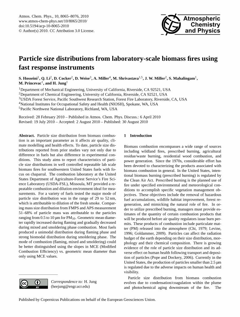
Atmos. Chem. Phys., 10, 8065–8076, 2010 www.atmos-chem-phys.net/10/8065/2010/ doi:10.5194/acp-10-8065-2010 © Author(s) 2010. CC Attribution 3.0 License. Atmospheric Chemistry and Physics Particle size distributions from laboratory-scale biomass fires using fast response instruments S. Hosseini 1 , Q. Li 2 , D. Cocker 2 , D. Weise 3 , A. Miller 4 , M. Shrivastava 1,5 , J. W. Miller 2 , S. Mahalingam 1 , M. Princevac 1 , and H. Jung 1 1 Department of Mechanical Engineering, University of California, Riverside, CA 92521, USA 2 Department of Chemical Engineering, University of California, Riverside, CA 92521, USA 3 USDA Forest Service, Pacific Southwest Research Station, Forest Fire Laboratory, Riverside, CA, USA 4 National Institutes for Occupational Safety and Health (NIOSH), Spokane, WA, USA 5 Pacific Northwest National Laboratory, Richland, WA, USA Received: 28 February 2010 – Published in Atmos. Chem. Phys. Discuss.: 6 April 2010 Revised: 19 July 2010 – Accepted: 2 August 2010 – Published: 30 August 2010 Abstract. Particle size distribution from biomass combus- tion is an important parameter as it affects air quality, cli- mate modelling and health effects. To date, particle size dis- tributions reported from prior studies vary not only due to difference in fuels but also difference in experimental con- ditions. This study aims to report characteristics of parti- cle size distributions in well controlled repeatable lab scale biomass fires for southwestern United States fuels with fo- cus on chaparral. The combustion laboratory at the United States Department of Agriculture-Forest Service’s Fire Sci- ence Laboratory (USDA-FSL), Missoula, MT provided a re- peatable combustion and dilution environment ideal for mea- surements. For a variety of fuels tested the major mode of particle size distribution was in the range of 29 to 52 nm, which is attributable to dilution of the fresh smoke. Compar- ing mass size distribution from FMPS and APS measurement 51–68% of particle mass was attributable to the particles ranging from 0.5 to 10 μm for PM 10 . Geometric mean diame- ter rapidly increased during flaming and gradually decreased during mixed and smoldering phase combustion. Most fuels produced a unimodal distribution during flaming phase and strong biomodal distribution during smoldering phase. The mode of combustion (flaming, mixed and smoldering) could be better distinguished using the slopes in MCE (Modified Combustion Efficiency) vs. geometric mean diameter than only using MCE values. Correspondence to: H. Jung ([email protected]) 1 Introduction Biomass combustion encompasses a wide range of sources including wildland fires, prescribed burning, agricultural residue/waste burning, residential wood combustion, and power generation. Since the 1970s, considerable effort has been devoted to characterizing the products associated with biomass combustion in general. In the United States, inten- tional biomass burning (prescribed burning) is regulated by the Clean Air Act. Prescribed burning is the planned use of fire under specified environmental and meteorological con- ditions to accomplish specific vegetation management ob- jectives. These objectives include the removal of hazardous fuel accumulations, wildlife habitat improvement, forest re- generation, and mimicking the natural role of fire. In or- der to utilize prescribed burning, managers must provide es- timates of the quantity of certain combustion products that will be produced before air quality regulators issue burn per- mits. These products of combustion include particulate mat- ter (PM) released into the atmosphere (Chi, 1979; Levine, 1996; Goldammer, 2009). Particles can affect the radiation budget of the earth depending on their size distribution, mor- phology and their chemical composition. There is growing evidence of the role of particle size distribution and its ad- verse effect on human health following transport and deposi- tion of particles (Pope and Dockery, 2006). Currently in the United States, the production of particles smaller than 2.5 μm is regulated due to the adverse impacts on human health and visibility. Particle size distribution from biomass combustion evolves due to condensation/coagulation within the plume and photochemical aging downstream of the fire. The Published by Copernicus Publications on behalf of the European Geosciences Union.
Transcript of Particle size distributions from laboratory-scale …...Particle size distributions from biomass...
Atmos. Chem. Phys., 10, 8065–8076, 2010www.atmos-chem-phys.net/10/8065/2010/doi:10.5194/acp-10-8065-2010© Author(s) 2010. CC Attribution 3.0 License.
AtmosphericChemistry
and Physics
Particle size distributions from laboratory-scale biomass fires usingfast response instruments
S. Hosseini1, Q. Li2, D. Cocker2, D. Weise3, A. Miller 4, M. Shrivastava1,5, J. W. Miller 2, S. Mahalingam1,M. Princevac1, and H. Jung1
1Department of Mechanical Engineering, University of California, Riverside, CA 92521, USA2Department of Chemical Engineering, University of California, Riverside, CA 92521, USA3USDA Forest Service, Pacific Southwest Research Station, Forest Fire Laboratory, Riverside, CA, USA4National Institutes for Occupational Safety and Health (NIOSH), Spokane, WA, USA5Pacific Northwest National Laboratory, Richland, WA, USA
Received: 28 February 2010 – Published in Atmos. Chem. Phys. Discuss.: 6 April 2010Revised: 19 July 2010 – Accepted: 2 August 2010 – Published: 30 August 2010
Abstract. Particle size distribution from biomass combus-tion is an important parameter as it affects air quality, cli-mate modelling and health effects. To date, particle size dis-tributions reported from prior studies vary not only due todifference in fuels but also difference in experimental con-ditions. This study aims to report characteristics of parti-cle size distributions in well controlled repeatable lab scalebiomass fires for southwestern United States fuels with fo-cus on chaparral. The combustion laboratory at the UnitedStates Department of Agriculture-Forest Service’s Fire Sci-ence Laboratory (USDA-FSL), Missoula, MT provided a re-peatable combustion and dilution environment ideal for mea-surements. For a variety of fuels tested the major mode ofparticle size distribution was in the range of 29 to 52 nm,which is attributable to dilution of the fresh smoke. Compar-ing mass size distribution from FMPS and APS measurement51–68% of particle mass was attributable to the particlesranging from 0.5 to 10 µm for PM10. Geometric mean diame-ter rapidly increased during flaming and gradually decreasedduring mixed and smoldering phase combustion. Most fuelsproduced a unimodal distribution during flaming phase andstrong biomodal distribution during smoldering phase. Themode of combustion (flaming, mixed and smoldering) couldbe better distinguished using the slopes in MCE (ModifiedCombustion Efficiency) vs. geometric mean diameter thanonly using MCE values.
Correspondence to:H. Jung([email protected])
1 Introduction
Biomass combustion encompasses a wide range of sourcesincluding wildland fires, prescribed burning, agriculturalresidue/waste burning, residential wood combustion, andpower generation. Since the 1970s, considerable effort hasbeen devoted to characterizing the products associated withbiomass combustion in general. In the United States, inten-tional biomass burning (prescribed burning) is regulated bythe Clean Air Act. Prescribed burning is the planned use offire under specified environmental and meteorological con-ditions to accomplish specific vegetation management ob-jectives. These objectives include the removal of hazardousfuel accumulations, wildlife habitat improvement, forest re-generation, and mimicking the natural role of fire. In or-der to utilize prescribed burning, managers must provide es-timates of the quantity of certain combustion products thatwill be produced before air quality regulators issue burn per-mits. These products of combustion include particulate mat-ter (PM) released into the atmosphere (Chi, 1979; Levine,1996; Goldammer, 2009). Particles can affect the radiationbudget of the earth depending on their size distribution, mor-phology and their chemical composition. There is growingevidence of the role of particle size distribution and its ad-verse effect on human health following transport and deposi-tion of particles (Pope and Dockery, 2006). Currently in theUnited States, the production of particles smaller than 2.5 µmis regulated due to the adverse impacts on human health andvisibility.
Particle size distribution from biomass combustionevolves due to condensation/coagulation within the plumeand photochemical aging downstream of the fire. The
Published by Copernicus Publications on behalf of the European Geosciences Union.

8066 S. Hosseini et al.: Particle size distributions from laboratory-scale biomass fires
particle size distribution can also differ by combustion phase(ignition/flaming/smoldering), fuel condition (live, dead andvarying moisture content), fuel configuration (dense vs. lightand plain vs. sloped terrain), and fuel types (foliage, log,branch). Due to the importance of particle size distributionand its impact on air quality, climate modeling and healtheffects, particle size distributions from diverse biomass com-bustion conditions have been reported (Janhall, 2009; Hayset al., 2005; Capes et al., 2008).
Particle size distributions from biomass burning have beenstudied for a variety of fuels (Le Canut, 1996; Posfai etal., 2003, 2004; Capes et al., 2008). A wide variety ofinstruments have been used to measure particle size distri-bution; Laser Optical Particle Counter, Aerosol Time-Of-Flight Mass Spectrometer (ATOFMS), Differential MobilityParticle Sizer (DMPS)(Hedberg et al., 2002; Sullivan et al.,2008), Scanning Mobility Particle Sizer (SMPS) (Hays et al.,2002; Hays et al., 2005), Transmission Electron Microscopy(TEM) analysis (Posfai et al., 2003; Posfai et al., 2004;Chakrabarty et al., 2006), Micro Orifice Uniform DepositImpactor (MOUDI) (Hays et al., 2005; Engling et al., 2009),and Passive Cavity Aerosol Spectrometer Probe (PCASP)(Capes et al., 2008).
Previous studies have shown a wide variation in particlesize distribution due to differing combustion and measure-ment conditions. Hays et al. (2002) reported unimodal distri-bution using a SMPS. They used open combustion of a fuelto simulate combustion of fuel in the field. They reported ge-ometric mean diameters between 0.1–0.2 µm. Due to the useof a small enclosure (28 m3), their particles may have grownby condensation and coagulation within the enclosure. LeCanut et al. (1996) measured particle size distribution usinga laser optical particle counter in their airborne study duringa savanna fire. They reported two mass modes: one in 0.2–0.3 µm and the other above 2 µm. Chakrabarty et al. (2006)measured particle size distribution from laboratory combus-tion of eight different fuels using SMPS and image analy-sis. Projected area equivalent diameter peaks ranged from30 to 200 nm for wet (moisture content (MC) = 20% on drymass basis) and dry (MC = 5–10%) fuels. Major mode diam-eter ranged between 40–45 nm for three out of six burns (seetheir Fig. 12) for dry fuels they tested. To authors’ knowledgenone of these previous studies captured the temporal evolu-tion of size distribution due to the relatively slow responserate of the instruments. For example, the SMPS requires 2min to measure one size distribution. Janhall et al. (2009) pa-rameterized particle number emissions by applying compli-cated fittings to published experimental data. They pointedout that well defined laboratory experiments should help val-idate their finding and enable a better understanding of parti-cle emission/formation mechanisms.
A study to characterize smoke emissions from prescribedburns in chaparral and Madrean oak woodlands in the south-western United States was initiated in 2008. Detailed charac-terization of gaseous and particulate emissions is being made
in laboratory and field settings. Changes in and transport ofemissions from the source downwind are being measured andmodeled for inclusion in air quality models such as CMAQ(Byun, 2006). The objective of this paper is to character-ize particle size distribution from the laboratory componentof the study. A suite of fast-response online instrumentswere applied to measure evolution of particle size distribu-tion from fire ignition to extinction to capture transient andintegrated characteristics of particle size distribution frombiomass burning. To the best of our knowledge, the cur-rent study reports fast time-dependent (1s interval) size dis-tribution of particle-phase emissions and their characteristicsfrom biomass burning in detail for the first time.
2 Experimental
2.1 Combustion lab facility
Experiments were conducted in the combustion laboratory atthe USDA Forest Service’s Fire Science Laboratory (FSL),Missoula, MT. A detailed description of the characteristicsof the facility can be found in Christian et al. (2004). Thefacility measures 12.5 m by 12.5 m and is 22 m in height.The combustion laboratory is exhausted via a 3.6 m diameterhood attached to a 1.6 m stack located in the center. Figure 1shows a schematic of the lab. The base of the hood is abovethe fuel bed. The stack extends from 2 m above the floor toall the way up through the ceiling. The lab is slightly pres-surized with pre-conditioned outside air to precisely controlthe temperature, and relative humidity. This ensures entrain-ment of all the produced emissions, making the conditionsideal for determining emissions factors. The air velocity inthe chimney was set at either 1.5 m/s or 3 m/s by controllingthe exhaust fan speed to maintain proper entrainment of freshair.
2.2 Particle measurement system
The sampling platform (Fig. 1) is located 17 m above thefloor surrounding the stack; this is where all particle mea-surement instruments were placed. Figure 2 shows schematicof the sampling system. First sampling flow was taken fromthe isokinetic sampling port installed at the height of the sam-pling platform in the stack. The sample flow was diluted us-ing a mini dilution tunnel at 1:13.5 ratio. The diluted aerosolflow wass directed to a PM10 impactor, then distributed toa Fast Mobility Particle Sizer (FMPS-model 3091, TSI1),an Aerodynamic Particle Sizer (APS-model 3321, TSI) anda Condensation Particle Counter (CPC Model 3775, TSI).Other online and offline instruments were used for physical
1The use of trade names is provided for informational purposesonly and does not constitute endorsement by the US Department ofAgriculture.
Atmos. Chem. Phys., 10, 8065–8076, 2010 www.atmos-chem-phys.net/10/8065/2010/

S. Hosseini et al.: Particle size distributions from laboratory-scale biomass fires 8067
Fig. 1. Schematic drawing of combustion laboratory, USDA ForestService Fire Sciences Laboratory, Missoula, MT. Detailed charac-teristics of the facility are described in Christian et al. (2004).
Stack PM10 impactor Diluter
CPC
FMPS
APSOP-FTIR
Fig. 2. Schematic of measurement system.
and chemical characterization of the particles but are not re-ported in this paper.
The Fast Mobility Particle Sizer Spectrometer (FMPS, TSIModel 3091) is capable of measuring mobility diameter ofthe particles. The instrument is made of two concentric cylin-ders (classification columns), a corona diffusion charger, and32 electrometers, which covers the particle size range of 5 to560 nm. The stream containing positively charged particlesflows along with sheath air. The high voltage between thetwo cylinders carries the particles from the side where theyare introduced to the other side that has the electrometers.Close to the top of the column, the particles with higher elec-trical mobility are collected, and further downstream the par-ticles with lower electrical mobility are collected (TSI man-
ual2). Electrical mobility,Z is defined as below
Z =neC
3πµgDm
Wheren, e, C, µg, Dm are number of charge, unit charge ofan electron, slip correction factor, gas viscosity and particlemobility diameter.
The aerodynamic diameterDa is the diameter of the unitdensity (ρp=1g/cm3) sphere that has the same settling ve-locity as the particle (Hinds, 1982). The Aerodynamic Par-ticle Sizer (APS, TSI Model 3321) is capable of measuringparticle size distributions in the size range between 0.5 and20 µm. The sample particles are accelerated as the carriergas flows through a converging nozzle. Due to the inertia,particles cannot accelerate as fast as the gas and the velocitylags that of the gas. Particle size is related to this velocity lagand that is measured at the nozzle exit when particles passthrough two closely spaced laser beams. The time of flightbetween the two laser beams is then used to calculate theaerodynamic diameter (Rader et al, 1990; Wang and John,1987). Chen et al. (1985) found a unique calibration curveexisted between a particle Stokes number and its velocitynormalized by the gas velocity.
The Stokes number is defined as
St =ρpD2
pVgC
9µgW
whereρp, Dp, Vg, C, µg, W are particle density, particle di-ameter, gas velocity, slip correction factor, gas viscosity anddiameter of the nozzle at the exit. The APS measured aero-dynamic diameter requires correction for non-Stokesian ef-fects when particle Reynolds diameter becomes greater than0.5 (Wang and John, 1987). A conversion of aerodynamicdiameter into mobility diameter requires a correction fac-tor involving dynamic shape factor and density of particles(Stober, 1971). The particle Reynolds numbers are reportedas 0.65, 4.8, 24 and 103 for diameters of 1.0, 2.1, 5, and15 µm by Wang and John (1987) for the APS at the nozzleflow velocity of 150 m/s. The current study does not aim tomeasure shape factor and density of particles for a conversionfrom aerodynamic to mobility diameter.
2.3 Gas measurement system
Every molecule has its own specific IR radiation absorp-tion pattern. Researchers have used this fact in Fast FourierInfraRed (FTIR) spectroscopy. If a beam of IR is passedthrough smoke, and the IR spectrum is recorded, the acquiredgraph will have peaks that are due to molecules present in thesmoke (Yokelson et al., 1997; Goode et al., 1999). The OP-FTIR instrument used in this study included a Bruker Matrix-M IR Cube spectrometer and a thermally stable open white
2http://www.tsi.com/uploadedFiles/ProductInformation/Literature/SpecSheets/3091FMPS.pdf
www.atmos-chem-phys.net/10/8065/2010/ Atmos. Chem. Phys., 10, 8065–8076, 2010

8068 S. Hosseini et al.: Particle size distributions from laboratory-scale biomass fires
cell. The white cell was positioned on the sampling platformapproximately 17 m above the fuel bed so that the open whitecell spanned the stack directly in the rising emissions stream.The white cell path length was set to 58 m. Several extensivetests were performed to optimize the many sampling param-eters, including duty cycle, sample frequency, and spectrom-eter options to choose a spectral resolution of 0.67 cm−1 andspectra were acquired every 1.5 s (four co-added spectra in1.5 s) beginning several minutes prior to the fire and contin-uously until the end of the fire. A pressure transducer andtwo temperature sensors were located adjacent to the opticalpath and were logged on the instrument computer and usedfor spectral analysis.
The Open-Path Fourier Transform infrared (OP-FTIR)spectrometer was used to monitor concentrations of CO andCO2 for this study. These concentrations were used to calcu-late a Modified Combustion Efficiency (MCE). MCE is de-fined as the amount of carbon released as CO2 divided bythe amount of carbon released as CO2 plus CO (Ward et al.,1996; Ward, 1993).
Since CO2 and CO account for about 95% of carbon re-leased during biomass combustion, the MCE is a good surro-gate for true combustion efficiency. Ward et al. (1993) classi-fiedcombustion conditions into three phases by MCE: flam-ing when MCE>0.97, mixed when 0.97≥MCE>0.85 andsmoldering when 0.85≥MCE>0.75.
2.4 Experimental fires
Fuel characterization and fuel bed configuration are very im-portant parameters to determine particle emissions and for-mations. Yet many previous studies are lacking this criticalinformation in their publications (Reid et al., 2005). In thepresent work, a total of 44 burns, composed of 8 differenttypes of wildland fuels (Table 1), were conducted. The fu-els were collected from California (Ft. Hunter-Liggett, Van-denberg Air Force Base) and Arizona (Ft. Huachuca). Thefuel types selected for study are composed primarily of liv-ing vegetation. The chaparral fuel type is actually mixturesof shrub species that grow together in the mediterranean cli-mate of California and Baja California. Many of the shrubspecies in this climate have developed similar physical char-acteristics to minimize water loss such as leaves with waxycuticles which pyrolyze at low temperatures (Susott, 1982).The shrub canopies are relatively porous which facilitates firespread. Fires burning in these fuel beds are typically intensewith relatively high rates of energy release. In the Madreanoak fuel types, the woodland type consists of oak trees withan understory of shrub species related to chaparral speciesand the savanna type consists of oak trees with an understoryof native and introduced grasses. Fuels were harvested fromthe three locations and shipped to Missoula where they werestored for several weeks prior to the experiments. During thistime, the fuels lost most of the moisture which was presentat the time of harvest.
(a)
(b)
Fig. 3. Two pictures showing fuel and fuel bed, before the fuel is liton fire.
A small amount of isopropyl alcohol (generally less than50 cc) was used initially to get a quick even ignition ofthe fuel bed. Eighteen of 44 of the southwestern fuel beds(chamise, ceanothus, manzanita, and California sagebrush– see Table 1) were ignited in this manner using a propanetorch. No alcohol was used to enhance ignition in the remain-ing fuel beds. With the exception of the masticated mesquitefuel type which was created by mowing down and grindingthe shrubs, the natural fuel beds tend to have a vertical orien-tation in the natural setting (Fig. 3a). We attempted to burnthe fuels in a vertical orientation with limited success so thefuels were oriented horizontally (Fig. 3b). Average consump-tion (mass basis) of the chamise/scrub oak fuels oriented ver-tically was 30%. Consumption of horizontally oriented fuelbeds increased to 90%. Bulk characteristics of the fuel bedsare found in Table 2. Average moisture content (oven-drymass basis, ASTM D4442-07) of the fuel beds at the timeof burning ranged from 4 to 33% which is similar to fuelmoistures in dead fuels. Moisture content in these live fuelsseldom decreases below 50% in the field. The initial oven-dry mass in the fuel beds ranged from 670 to 4630 g. Bulk
Atmos. Chem. Phys., 10, 8065–8076, 2010 www.atmos-chem-phys.net/10/8065/2010/

S. Hosseini et al.: Particle size distributions from laboratory-scale biomass fires 8069
Table 1. Fuel type species composition and abbreviations.
Fuel type Fuel Code Plant Species
Chamise/scrub oak CHS Adenostomafasciculatum, QuercusberberidifoliaCeanothus CEA CeanothusleucodermisCoastal sage scrub COS Salvia mellifera, Ericameriaericoides, Artemisia californicaCalifornia sagebrush CAS Artemisia californica, EricameriaericoidesManzanita MAN Arctostaphylosrudis, ArctostaphylospurissimaOak savanna OAS Quercusemoryi, EragrostislehmannianaOak woodland OAW Quercusemoryi, ArctostaphylospungensMasticated mesquite MES Prosopisvelutina, Baccharissarothroides
Table 2. Fuel and bed properties.
Fueltype n Moisture content (%) Fuel bed dry mass (g) Bulk density (km/3) Packing ratioa Consumption (%)
Chamise/ScrubOak (CHS) 6 11.9 2079 8.6 0.015 38Ceanothus (CEA) 6 10.2 2007 5.8 0.010 54Coastal Sage Scrub (COS) 5 9.3 2299 6.0 0.010 95California Sagebrush (CAS) 6 9.0 2460 6.4 0.011 93Manzanita (MAN) 6 12.6 2906 7.6 0.013 94Oak Savanna (OAS) 5 14.3 2788 7.3 0.012 91Oak Woodland (OAW) 5 32.8 2054 5.3 0.009 95Masticated Mesquite (MES) 5 4.3 1831 14.3 0.024 92
a Packing ratio = bulk density/particle density. Assumed particle density of 593 kg m−3 (average from Countryman, 1982).
density of the fuel beds ranged from 5.8 to 14 kg/m3 and thepacking ratio (defined as the ratio of fuel bed bulk densityto fuel particle density) ranged from 0.010 to 0.024. Thesepacking ratios are similar to those reported for laboratory firespread experiments (Weise et al., 2005), but they are 1 to 2orders of magnitude larger than packing ratios observed inthe field which indicates the fuel beds were less porous thannatural fuel beds. While our initial intent was to burn fuelbeds similar to those found naturally, the fuel beds in the labexperiment were much drier with higher bulk densities thanthe fuel types they represent.
3 Results and discussion
3.1 Particle size distribution from 7 to 520 nm measuredby FMPS
Figure 4a shows averaged particle size distribution for dif-ferent fuels as measured by FMPS. The size distribution isaveraged over the time from ignition to the end of sampling(absolute CO concentration 1 ppm) and over at least threeburn replicates for each fuel type. Averaged size distribu-tions were unimodal for many fuel types. Interestingly, afew fuel types showed biomodal distributions, with the mi-nor (meaning lower concentration) mode around 10 nm. Themajor mode varies from 29 to 52 nm for fuels tested. This is a
very narrow range considering the diverse fuels tested. Con-sistent technique was used to minimize experimental errorsin order to detect differences between species. The similarityof the size distribution among fuels tested can be attributableto the systematic burning and sampling method.The combus-tion facility in Missoula was designed to divert all the gen-erated smoke into the chimney. This allows enough dilutionof the particles so that particle sizes measured and reportedin this facility are smaller than those from other studies.Chakrabarty et al. (2006) used the same combustion facil-ity in Missoula for their experiment. They reported particleCount Median Diameter (CMD) varying from 30 to 70 nmfor dry fuels (sage brush, poplar wood, ponderosa pine wood,ponderosa pine needles, white pine needles, Montana grass,dambo grass, tundra core) but they found the CMD increasesto 120–140 nm for wet fuels (tundra core and Montana grass)from their SEM measurement. Hays et al. (2005) measuredsize distribution from open burning of agricultural biomass(wheat straw). The open burning was conducted in an enclo-sure and the particles were diluted from 1:25 to 36 and mea-sured by a SMPS. They reported a biomodal distribution andsuggested that one mode is characterized by nucleation whilethe other represents an accumulation mode. The modes intheir size distributions were around 100 nm. Their measuredSMPS scans take 60 to 120 s. Considering characteristics ofbiomass burning this is not fast enough to capture the tran-sient phenomena. The background particle size distribution
www.atmos-chem-phys.net/10/8065/2010/ Atmos. Chem. Phys., 10, 8065–8076, 2010

8070 S. Hosseini et al.: Particle size distributions from laboratory-scale biomass fires
(a) (b)
(c) (d)
(e) (f)
Fig. 4. Particle size distributions corresponding to(a)whole burn (linear)(b) whole burn (log-log)(c)Flaming,(d) Mixed, and(e)Smolderingphases(f) presents background levels measured by FMPS(g) variation of measurements.
Atmos.Chem. Phys., 10, 8065–8076, 2010 www.atmos-chem-phys.net/10/8065/2010/

S. Hosseini et al.: Particle size distributions from laboratory-scale biomass fires 8071
was obtained by averaging size distributions measured beforeignition for seven burns which were conducted consecutivelyin one experimental day and plotted with averaged size distri-butions in log scale as shown in Fig. 4b. Figure 4b also showsthat particle concentration decreased sharply above 200 nm.
While some other studies report combustion conditionsof biomass burn only by using integrated or averaged MCEover the whole burn, we attempted to segregate the mode ofcombustion during each burn using instantaneous MCE valueand other indicators (i.e. slopes in MCE vs geometric meandiameter curve). The average size distributions of Fig. 4aand b were segregated into three burning conditions: flam-ing, mixed and smoldering by MCE. This division was doneby plotting geometric mean diameter change as a functionof MCE instead of using only Ward and Radke’s criteria byMCE value. Details of this will be discussed in later section.The majority of particles were emitted during flaming there-fore the shapes of size distributions during flaming were sim-ilar to that of the average of the whole burn (Fig. 4c). (Noteour presentation of data in Fig. 4 is time based while somestudies report particle emission per fuel mass.) Mixed phase,whichconsists of flaming and smoldering, shows unimodaldistribution with the mode ranges from 30 to 50 nm (Fig. 4d).The particle concentration was lower than that of flaming bya factor of 5 roughly. The change between flaming and mixedmode could be observed clearly from our video recording ofall burns. The size of flames was decreased noticeably at thebeginning of the mixed phase compared to the flaming phase.The flame was still clearly visible during the mixed phase.
Size distribution during smoldering showed a bimodal dis-tribution for all fuel types at around 10 nm (Fig. 4e). A pos-sible explanation for this is nucleation of volatile particlesas the burnt gas temperature cooled down. The particle con-centration during smoldering was two orders of magnitudelower than during the flaming phase. Note that this is time-based not fuel mass-based. Analysis of fuel mass-based re-sults will be reported in another paper. Figure 4f shows back-ground particle size distribution change during a day. Thebackground concentrations (Fig. 4f) are much lower than ourmeasured particle concentration during the burn (Fig. 4c, d,e), which ensures that background particles did not interferewith our measurements. Figure 4g shows variation of FMPSnumber distribution measurement for the fuel of oak savanna.Thick solid line represents average of six burns and shadedarea shows variation. Table 3 shows the geometric diameterand standard deviation of size distributions for fuels tested.Similarity between geometric mean diameter for the nine fueltypes is illustrated in Table 4. Notice that the standard devia-tions of the distributions are similar. Several of the chaparralfuel types had similiar geometric mean diameters and the twoMadrean oak fuel types were also similar.
Table 3. Geometric mean diameter and the geometric standard de-viations.
Fueltype In total
Dg(nm) σ
CaliforniaSagebrush (CAS) 50.72 1.66Ceanothus (CEA) 39.67 1.64Chamise/Scrub Oak (CHS) 52.30 1.62Coastal Sage Scrub (COS) 45.30 1.62Manzanita (MAN) 39.20 1.62Masticated Mesquite (MES) 34.00 1.58Oak Savanna (OAS) 25.00 1.76Oak Woodland (OAW) 29.00 1.67
Table 4.Species effects on particle size distribution.
FuelType CAS CEA CHS COS MAN MES OAS OAW
CAS N1 Y Y N N N NCEA N Y Y Y N NCHS N N N N NCOS Y N N NMAN Y N NMES N YOAS Y
1 Y indicates mean geometric diameter of fuel type 1±2σoverlaps with mean geomet-ric diameter of fuel type 2±2σ.
3.2 Particle size distribution from 0.5 to 20 µmmeasured by APS
Figure 5a shows time and cycle averaged particle size dis-tributions from APS measurements. This was done to de-termine whether concentration of large particles were higherthan background levels of aerosol by number and by volume.It has been reported that mass mean diameter is as large as0.5 µm (or 500 nm) for aged particles from biomass burning(Reid et al., 2005). Most of these previous measurementswere performed optically by aircraft measurement. Parti-cles larger than 100 nm in mobility diameter were reportedby previous studies which measured size distribution in thefield. However, smaller particle mode was reported for par-ticles measured in the lab (Hays et al., 2005; Keshtkar andAshbaugh, 2007). This can be attributed to immediate di-lution which prevents further coagulation and condensation.Regardless, particles larger than 0.5 µm were measured usingAPS to determine whether there was any noticeable numberor mass of particles in this size range from freshly dilutedbiomass smoke. The particle number distribution (Fig. 5a)showed that the concentrations are orders of magnitude lowercompared to the concentrations of small particles measuredby FMPS. Log conversion of Fig. 5a illustrated that thesmoke particle distributions were greater than background.Background distributions (Fig. 5f) measured between each
www.atmos-chem-phys.net/10/8065/2010/ Atmos. Chem. Phys., 10, 8065–8076, 2010

8072 S. Hosseini et al.: Particle size distributions from laboratory-scale biomass fires
(a) (b)
(c) (d)
(e) (f)
Fig. 5. Aerodynamic particle size distribution measured by APS for different phases(a) whole burn(linear)(b) whole burn(log-log)(c)Flaming(d) Mixed (e)Smoldering, and(f) corresponds to background concentration
burn during a day show that they do not vary much comparedto that of small size particles (Fig. 4f). This validated that ourAPS measurements were not interfered by background parti-cle size distribution. The average size distributions of Fig. 5
were separated by combustion phases using the same methodused with the FMPS size distribution. Particles larger than0.5µm were emitted mostly during flaming and mixed phasesof combustion. Emissions during the smoldering phase were
Atmos. Chem. Phys., 10, 8065–8076, 2010 www.atmos-chem-phys.net/10/8065/2010/

S. Hosseini et al.: Particle size distributions from laboratory-scale biomass fires 8073
Fig. 6. Particle number and mass size distributions correspondingto a typical burn, also the background concentration.
lower by at least a factor of 4 incomparison to peak concen-trations.
The mass distributions were compared between large andsmall particles measured by APS and FMPS. The numberof fractal-like particles for the size greater than 0.5 µm wasinsignificant based on our TEM measurement (images notshown in this paper). A range of particle densities was cho-sen to assess uncertainties in mass distribution taking intoaccount the non-Stokesian effects. Figure 6 shows that themass larger than 0.5 µm attribute to 51–68% of total volumemeasured by APS and FMPS when particle density range of0.8∼2.5 was assumed for non-Stokesian correction with theAPS measurement. Note that the dilution was applied for allonline aerosol measurements. RH of dilution air was main-tained at 16.5±4%. Note the size distribution by APS is inaerodynamic diameter while that by FMPS is in mobility di-ameter.
3.3 Evolution of particle size distribution (FMPS+APS)
It is extremely difficult to identify what determines evolutionof particle distribution from biomass burning due to the largevariability in fuel composition, fuel humidity, fuel bed ar-rangement and the nature of turbulent combustion. Thereforemost previous studies reported either time-integrated resultsor snap shots of transient phenomenon. In order to under-stand the evolution of particle size distribution, it is instruc-tive to examine Fig. 7 which shows the evolution of parti-cle size distribution for a burn from initial ignition until ex-tinction. This temporal resolution is possible due to the fastscanning ability of the FMPS and the APS (1 scan per sec-ond). The data showed that particle concentration reached amaximum during the flaming phase (confirmed by CO andCO2 data) and diminished to lower concentration either inunimodal or bimodal distributions. Right after ignition CO2
Fig. 7. (a)Modified Combustion Efficiency (MCE); CorrespondingAPS(b) and FMPS(c) contour graphs showing particle number sizedistributions.
concentration increases and that leads to increase in MCE.After the MCE reaches nearly one it starts to decrease be-cause1 CO2/1 CO decreases as shown in Fig. 7a. Dur-ing smoldering phase,1 CO2/1CO increases again mainlydue to decrease in1 CO, which leads to increase of MCEvalue. The MCE value reaches a plateau toward the endof the smoldering phase. During the flaming phase signif-icant particle emissions occur for the size range measuredby both instruments (FMPS and APS). It is important tonote that emissions of ultrafine particles (Dp<100 nm) re-duce significantly as the combustion phase progresses fromflaming, mixed to smoldering phase. On the other hand highconcentration of particles between 0.5 and 1 µm range per-sist during flaming, mixed phase and even past smolderinguntil 400 s in Fig. 7b. It is noteworthy that near the end
www.atmos-chem-phys.net/10/8065/2010/ Atmos. Chem. Phys., 10, 8065–8076, 2010

8074 S. Hosseini et al.: Particle size distributions from laboratory-scale biomass fires
Fig. 8. Geometric Mean Diameter as a function of time for a fewburns:(a) Manzanita (MAN)(b) Mesquite (MES)(c) Coastal Sage(COS).
of the smoldering phase ultrafine particles show a bimodaldistribution clearly (see Fig. 7c). Values of peak concentra-tion measured by FMPS were at least three to four orders ofmagnitude higher than APS concentrations during the flam-ing and mixed phases. Likewise, the evolution of geometricmean diameter was plotted for a few burns as illustrated inFig. 8. These results revealed that the geometric mean di-ameter increases rapidly during flaming phase and decreasedduring mixed and smoldering phases. In Fig. 9, MCE wasplotted as a function of geometric diameter for three differ-ent fuels. Ward and Radke’s (1993) MCE criteria gives aguideline to distinguish different phase of combustion but itfails to give accurate distinction at specific MCE values. Forexample smoldering mode starts at different MCE values of0.82, 0.76 and 0.83 for the different burns in Fig. 9a, b, c. Asthe combustion of biomass is always dynamic instead of be-ing steady state, either combustion or emissions parametersshould evolve at a different rate and/or direction at differ-ent phase of combustion. When we plotted the MCE valueagainst geometric mean diameter, we found that the distinc-tion between different phases of combustion could be moreclearly seen. This was also confirmed by comparing videorecords of the burn with Fig. 9. The geometric mean diame-ter increased rapidly during the flaming condition when MCEwas>0.97. However the MCE value for the mixed phasecould become smaller than what Ward and Radke (1993) de-fine. The geometric mean diameter decreased during bothmixed and smoldering conditions. While the MCE decreasedas the mixed phase proceeded, the MCE value increased asthe smoldering phase proceeded. As a result one can distin-guish mixed phase combustion from smoldering phase com-bustion based on the slope change in MCE vs. goemetricmean diameter graph.
(a)
(b)
(c)
Fig. 9. MCE vs. Geometric Mean Diameter for three typical burns.
Atmos. Chem. Phys., 10, 8065–8076, 2010 www.atmos-chem-phys.net/10/8065/2010/

S. Hosseini et al.: Particle size distributions from laboratory-scale biomass fires 8075
4 Conclusions
This paper presented particle size distributions measured bya suite of fast-response online instruments for laboratory-scale biomass fires for a variety of southwestern US fueltypes. The instruments measured evolution of particle sizedistribution from fire ignition to extinction to capture tran-sient and integrated characteristics of the particle size distri-bution. Time-averaged particle size distributions were seg-regated into three combustion phases: flaming, mixed andsmoldering. The major mode of particle size distributionwas in the range of 29 to 52 nm for the cycle-averaged dis-tributions. These are much smaller diameters compared toprevious studies. The difference from previous studies wasattributed to dilution of the fresh smoke in the current study.Time-averaged particle concentrations were highest duringthe flaming phase and gradually decreased during mixed andsmoldering phases. Comparing mass size distribution fromthe FMPS and APS measurements, 51–68% of particle masswas attributable to the particles ranging from 0.5 to 10 µm forPM10. Geometric mean diameter rapidly increased duringflaming combustion and gradually decreased during mixedand smoldering phase combustion. Particle size distributionwas unimodal for most fuel types during the flaming phaseand strongly biomodal during the smoldering phase. Theslopes of the linear plots of MCE versus geometric mean di-ameter appear to better separate the combustion phases thansimply using the value of MCE. Given the wide use of MCEalone to define combustion phases, additional measurementof particulate matter from biomass burning using fast re-sponse instruments is recommended.
Supplementary material related to thisarticle is available online at:http://www.atmos-chem-phys.net/10/8065/2010/acp-10-8065-2010-supplement.pdf.
Acknowledgements.Funding for this study was provided by theUS Department of Defense Strategic Environmental Researchand Development Program as projects SI-1647, SI-1648, andSI-1649. We appreciate the assistance of personnel at USMCCamp LeJuene, US Army Ft. Huachuca, Ft. Hunter-Liggett, Ft.Benning, and Vandenberg Air Force Base in selecting fuel typesfor study and fuel samples for burning. Authors are grateful toRobert Yokelson and Ian Burling for FTIR data and WeiMinHaoand Shawn Urbanski; Cyle Wold, Joey Chong, Trevor Maynardand Emily Lincoln for their help.
Edited by: H. Moosmuller
References
Byun, D. W. and Schere, K. L.: Review of Governing equa-tions, Computational Algorithms, and Other Components of theModels-3 Community Multi-scale Air Quality (CMAQ) Model-ing Systems, Appl. Mech. Rev., 59, 51–77, 2006.
Capes,G., Johnson, B., McFiggans, G., Williams, P. I., Haywood,J., and Coe, H.: Aging of biomass burning aerosols over WestAfrica: Aircraft measurements of chemical composition, mi-crophysical properties, and emission ratios, J. Geophys. Res.-Atmos., 113, D00C15, doi:10.1029/2008JD009845, 2008.
Chakrabarty, R. K., Moosmuller, H., Garro, M. A., Arnott, W. P.,Walker, J., Susott, R. A., Babbitt, R. E., Wold, C. E., Lincoln,E. N., and Hao, W. M.: Emissions from the laboratory combus-tion of wildland fuels: Particle morphology and size, J. Geophys.Res.-Atmos., 111, D07204, doi:10.1029/2005JD00665, 2006.
Chen,B. T., Cheng, Y. S., and Yeh, H. C.: Performance of a TSIAerodynamic Particle Sizer, Aerosol Sci. Technol., 4, 89–97,1985.
Chi, C. T., Horn, D. A., Reznik, R. B., Zanders, D. L., Opferkuch,R. E., Nyers, J. M., Pierovich, J. M., Lavdas, L. G., Mcmahon,C. K., Nelson, R. M., Johansen, R. W., and Ryan, P. W.: Sourceassessment: prescribed burning, state of the art, US Environmen-tal Protection Agency, EPA (US) Report EPA-600/2-79-019h,November 1979.
Christensen,N. L.: Vegetation of the southeatern costal plain, in:North American Terrestial Vegetation, edited by: Barbour, M.G., W. D. B., Cambridge University Press, UK, 397–449, 1999.
Christian,T. J., Kleiss, B., Yokelson, R. J., Holzinger, R., Crutzen,P. J., Hao, W. M., Shirai, T., and Blake, D. R.: Com-prehensive laboratory measurements of biomass-burning emis-sions: 2. First intercomparison of open-path FTIR, PTR-MS,and GC-MS/FID/ECD, J. Geophys. Res.-Atmos., 109, D02311,doi:10.1029/2003JD003874, 2004.
Countryman,C. M.: Physical characteristics of some northern Cali-fornia brush fuels, USDA Forest Serivce, Pacific Southwest For-est and Range Experiment Station, General Technical Report, 2–4, 1982.
Engling, G., Lee, J. J., Tsai, Y. W., Lung, S. C. C., Chou, C. C.K., and Chan, C. Y.: Size-Resolved Anhydrosugar Compositionin Smoke Aerosol from Controlled Field Burning of Rice Straw,Aerosol Sci. Technol., 43, 662–672, 2009.
Goldammer, J. G., Statheropoulos, M., and Andreae, M. O.,Goldammer, J. G., Statheropoulos, M., and Andreae, M. O.: Im-pacts of vegetation fire emissions on the environment, humanhealth, and security: a global perspective, edited by: Bytnerow-icz, A., Arbaugh, M., Riebau, A., and Andersen, C., WildlandFires and Air Pollution, Elsevier, 8, 3–36, doi:10.1016/S1474-8177(08)00001-62009, 2008.
Goode,J. G., Yokelson, R. J., Susott, R. A., and Ward, D. E.: Trace-gasmissions from laboratory biomass fires measured by Fouriertransforminfrared spectroscopy: Fires in grass and surface fuels,J. Geophys. Res., 104, 21237–21245, 1999.
Hays,M. D., Geron, C. D., Linna, K. J., Smith, N. D., and Schauer,J. J.: Speciation of gas-phase and fine particle emissions fromburning of foliar fuels, Environ. Sci. Technol., 36, 2281–2295,2002.
Hays,M. D., Fine, P. M., Geron, C. D., Kleeman, M. J., and Gullett,B. K.: Open burning of agricultural biomass: Physical and chem-ical properties of particle-phase emissions, Atmos. Environ., 39,
www.atmos-chem-phys.net/10/8065/2010/ Atmos. Chem. Phys., 10, 8065–8076,2010

8076 S. Hosseini et al.: Particle size distributions from laboratory-scale biomass fires
6747–6764, 2005.Hedberg, E., Kristensson, A., Ohlsson, M., Johansson, C., Johans-
son, P. A., Swietlicki, E., Vesely, V., Wideqvist, U., and Wester-holm, R.: Chemical and physical characterization of emissionsfrom birch wood combustion in a wood stove, Atmos. Environ.,36, 4823–4837, 2002.
Hinds, W. C.: Aerosol Technology: Properties, Behaviour, andMeasurement of Airborne Particles, Wiley Interscience, NewYork, USA, 316–349, 1982.
Keeley, J. E.: Chaparral, in: North American Terrestrial Vegeta-tion, edited by: Barbour, M. G. and Billing, W. D., CambridgeUniversity Press, NY, USA, 397–448, 1999.
Janhall, S., Andreae, M. O., and Poschl, U.: Biomass burningaerosol emissions from vegetation fires: particle number andmass emission factors and size distributions, Atmos. Chem.Phys., 10, 1427–1439, doi:10.5194/acp-10-1427-2010, 2010.
Keshtkar, H. and Ashbaugh, L. L.: Size distribution of polycyclicaromatic hydrocarbon particulate emission factors from agricul-tural burning, Atmos. Environ., 41, 2729–2739, 2007.
Levine, J. S.: Biomass Burning and Global Change, MIT Press,131–139, 1996.
Le Canut, P., Andreae, M. O., Harris, G. W., Wienhold, F.G., and Zenker, T.: Airborne studies of emissions from sa-vanna fires in southern Africa, J. Geophys. Res.-Atmos., 8483,doi:10.1029/2002jd002291, 1996.
Pope, C. A. and Dockery, D. W.: Health effects of fine particulateair pollution: Lines that connect, J. Air Waste Manage., 56, 709–742, 2006.
Posfai, M., Simonics, R., Li, J., Hobbs, P. V., and Buseck,P. R.: Individual aerosol particles from biomass burning insouthern Africa: 1. Compositions and size distributions of car-bonaceous particles, J. Geophys. Res.-Atmos., 108(D13), 8483,doi:10.1029/2002JD002291, 2003.
Posfai, M., Gelencser, A., Simonics, R., 5 Arato, K., Li, J., Hobbs,P. V., and Buseck, P. R.: Atmospheric tar balls: Particles frombiomass and biofuel burning, J. Geophys. Res.-Atmos., 109,D22302, doi:10.1029/2008jd010216, 2004.
Rader, D. J. and McMurry, P. H.: Application of the Tandem Differ-ential Mobility Analyzer to studies of droplet growth and evapo-ration, J. Aerosol Sci., 17, 771–788, 1986.
Reid,J. S., Koppmann, R., Eck, T. F., and Eleuterio, D. P.: A reviewof biomass burning emissions part II: intensive physical proper-ties of biomass burning particles, Atmos. Chem. Phys., 5, 799-825, doi:10.5194/acp-5-799-2005, 2005.
Stober, W. A.: A note on the aerodynamic diameter and the mobilityof non-spherical aerosol particles, J. Aerosol Sci., 2, 453–456 ,1971.
Sullivan, A. P., Holden, A. S., Patterson, L. A., McMeeking, G.R., Kreidenweis, S. M., Malm, W. C., Hao, W. M., Wold, C. E.,and Collett, J. L.: A method for smoke marker measurementsand its potential application for determining the contribution ofbiomass burning from wildfires and prescribed fires to ambientPM2.5 organic carbon, J. Geophys. Res.-Atmos., 113, D22302,doi:10.1029/2008JD010216, 2008.
Susott,R. A.: Characterization of the thermal properties of forestfuels by combustible gas analysis., Forest Sci., Society of Amer-ican Foresters, 28, 404–420(17) 1982.
Wang, H. and John, W.: Particle Density Correction for the Aero-dynamic Particle Sizer, Aerosol Sci. Technol., 6, 191–198, 1987.
Ward, D. E., Hao, W. M., Susott, R. A., Babbitt, R. E., Shea, R. W.,Kauffman, J. B., and Justice, C. O.: Effect of fuel composition oncombustion efficiency and emission factors for African savannaecosystems, J. Geophys. Res.-Atmos., 101, 23569–23576, 1996.
Ward, D. E. and Radke, L. E.: Emission measurements from veg-etation fires: a comparativeevaluation of methods and results,in: Fire in Environment. The Ecological, Atmospheric and Cli-matic Importance of Vegetation Fires, edited by: Crutzen, P. J.and Goldammer, J. G., John Wiley and Sons, New York, USA,53–76, 1993.
Weise, D. R., Zhou, X. Y., Sun, L. L., and Mahalingam, S.: Firespread in chaparral – ’go or no-go?’, Int J. Wildland Fire, 14,99–106, 2005.
Yokelson, R. J., Ward, D. E., Susott, R. A., Reardon, J., and Griffith,D. W. T.: Emissions from smoldering combustion of biomassmeasured byopen-path Fourier transform infrared spectroscopy,J. Geophys. Res., 102, 18865–18877, 1997.
Atmos. Chem. Phys., 10, 8065–8076, 2010 www.atmos-chem-phys.net/10/8065/2010/

Atmos. Chem. Phys., 10, 8511, 2010www.atmos-chem-phys.net/10/8511/2010/doi:10.5194/acp-10-8511-2010© Author(s) 2010. CC Attribution 3.0 License.
AtmosphericChemistry
and Physics
Corrigendum to
“Particle size distributions from laboratory-scale biomass fires usingfast response instruments” published in Atmos. Chem. Phys., 10,8065–8076, 2010
S. Hosseini1, Q. Li2, D. Cocker2, D. Weise3, A. Miller 4, M. Shrivastava1,5, J. W. Miller 2, S. Mahalingam1,M. Princevac1, and H. Jung1
1Department of Mechanical Engineering, University of California, Riverside, CA 92521, USA2Department of Chemical Engineering, University of California, Riverside, CA 92521, USA3USDA Forest Service, Pacific Southwest Research Station, Forest Fire Laboratory, Riverside, CA, USA4National Institutes for Occupational Safety and Health (NIOSH), Spokane, WA, USA5Pacific Northwest National Laboratory, Richland, WA, USA
The last graph in Fig. 4, p. 8070 has a label “(g)” which isnot printed. This graph corresponds to Fig. 4g – “Variationof measurements”.
In addition, there is no supplementary material related tothis article as stated in p. 8075.
The authors wish to apologize for these errors.
Correspondence to:H. Jung([email protected])
Publishedby Copernicus Publications on behalf of the European Geosciences Union.


Atmos. Chem. Phys., 10, 8511, 2010www.atmos-chem-phys.net/10/8511/2010/doi:10.5194/acp-10-8511-2010© Author(s) 2010. CC Attribution 3.0 License.
AtmosphericChemistry
and Physics
Corrigendum to
“Particle size distributions from laboratory-scale biomass fires usingfast response instruments” published in Atmos. Chem. Phys., 10,8065–8076, 2010
S. Hosseini1, Q. Li2, D. Cocker2, D. Weise3, A. Miller 4, M. Shrivastava1,5, J. W. Miller 2, S. Mahalingam1,M. Princevac1, and H. Jung1
1Department of Mechanical Engineering, University of California, Riverside, CA 92521, USA2Department of Chemical Engineering, University of California, Riverside, CA 92521, USA3USDA Forest Service, Pacific Southwest Research Station, Forest Fire Laboratory, Riverside, CA, USA4National Institutes for Occupational Safety and Health (NIOSH), Spokane, WA, USA5Pacific Northwest National Laboratory, Richland, WA, USA
The last graph in Fig. 4, p. 8070 has a label “(g)” which isnot printed. This graph corresponds to Fig. 4g – “Variationof measurements”.
In addition, there is no supplementary material related tothis article as stated in p. 8075.
The authors wish to apologize for these errors.
Correspondence to:H. Jung([email protected])
Published by Copernicus Publications on behalf of the European Geosciences Union.