PARTICIPATION OF

COMBINED CYCLE POWER PLANTS TO

POWER SYSTEM FREQUENCY CONTROL: MODELING AND APPLICATION

A THESIS SUBMITTED TO THE GRADUATE SCHOOL OF NATURAL AND APPLIED SCIENCES

OF MIDDLE EAST TECHNICAL UNIVERSITY

BY

OĞUZ YILMAZ

IN PARTIAL FULFILLMENT OF THE REQUIREMENTS FOR

THE DEGREE OF MASTER OF SCIENCE IN

ELECTRICAL AND ELECTRONICS ENGINEERING

APRIL 2006

Approval of the Graduate School of Natural and Applied Sciences.

Prof. Dr. Canan Özgen

Director

I certify that this thesis satisfies all the requirements as a thesis for the degree of Master of Science.

Prof. Dr. İsmet Erkmen Head of Department

This is to certify that we have read this thesis and that in our opinion it is fully adequate, in scope and quality, as a thesis for the degree of Master of Science.

Prof. Dr. İsmet Erkmen Supervisor

Examining Committee Members Prof. Dr. Önder Yüksel (METU, EE)

Prof. Dr. İsmet Erkmen (METU, EE)

Prof. Dr. Erol Kocaoğlan (METU, EE)

Prof. Dr. Arif Ertaş (METU, EE)

Abdullah Nadar (MS) (TUBITAK-BILTEN)

iii

I hereby declare that all information in this document has been obtained and presented in accordance with academic rules and ethical conduct. I also declare that, as required by these rules and conduct, I have fully cited and referenced all material and results that are not original to this work.

Name, Last name: Oğuz Yılmaz

Signature:

iv

ABSTRACT

PARTICIPATION OF

COMBINED CYCLE POWER PLANTS TO

POWER SYSTEM FREQUENCY CONTROL: MODELING AND APPLICATION

Yılmaz, Oğuz

MS, Department of Electrical and Electronics Engineering

Supervisor: Prof. Dr. İsmet Erkmen

April 2006, 66 Pages This thesis proposes a method and develops a model for the participation of a

combined cycle power plant to power system frequency control.

Through the period of integration to the UCTE system, (Union for Coordination of

Transmission of Electricity in Europe) frequency behavior of Turkey’s grid and

studies related to its improvement had been a great concern, so is the reason that

main subject of my thesis became as “Power System Frequency Control”.

Apart from system-wide global control action (secondary control); load control loops

at power plants, reserve power and its provision even at the minimum capacity

generation stage, (primary control) are the fundamental concerns of this subject.

The adjustment of proper amount of reserve at the power plants, and correct system

response to any kind of disturbance, in the overall, are measured by the quality of the

frequency behaviour of the system.

v

A simulator that will simulate a dynamic gas turbine and its control system model,

together with a combined cycle power plant load controller is the outcome of this

thesis.

Keywords __ combined cycle power plant, gas turbine, governor, reserve power, plant

outer control loop.

vi

ÖZ

KOMBİNE ÇEVRİM ENERJİ SANTRALLARININ ŞEBEKE FREKANSI KONTROLUNE KATILIMI:

MODELLENMESI VE UYGULAMASI

Yılmaz, Oğuz

Yüksek Lisans, Elektrik-Elektronik Mühendisliği Bölümü

Tez Yöneticisi: Prof. Dr. İsmet Erkmen

Nisan 2006, 66 Sayfa

Bu tez, kombine çevrim elektrik santralının şebeke frekansı kontrolune doğru

katılımının nasıl olması gerektiği üzerine, bir metot önerisi ve model uygulaması

içermektedir.

Mezuniyetimden bu yana, UCTE sistemine entegrasyon çalışmalarının sürdürüldüğü

bu dönem boyunca, Türkiye şebekesinin frekansının davranışı ve iyileştirilmesi

yönünde yapılan çalışmalar her zaman gündemin üst sırasında yer aldı. Bu sebeple de

lisansüstü eğitimimin başlangıcında, tez çalışmamın ana konusu “Enterkonnekte

Sistemlerde Frekans Kontrolu” olarak belirlendi.

Santrallardaki güç kontrol döngülerinin analizinin ve rezerv güç miktarının

sürekliliğinin; bu gücün en küçük üretim biriminde bile, uygun şekilde, gerektiğinde

sisteme temin edilebilir olmasının, bu konunun en temel kavramları olduğu

söylenebilir.

vii

Sistemin geneli için, santrallarda rezerv güç miktarının yeterince ayarlanıp

ayarlanmadığı ve herhangi bir frekans sapmasına verilen kollektif cevabın

doğruluğu, şebeke frekansının davranış karakteristiği incelenerek değerlendirilir.

Bu tez çalışmasının sonucunda, dinamik bir gaz türbini ve kontrol sistemi modeli ile

birlikte, doğalgaz kombine çevrim santrallarında kullanılabilecek yük denetleyicisi

modelini içeren bir simulasyon elde edilmiştir.

Anahtar Kelimeler __ kombine çevrim santralı, gaz türbini, yük kontrolu, rezerv güç,

santral dış kontrol döngüleri.

viii

TABLE OF CONTENTS

PLAGIARISM ……………………………………………………………….iii

ABSTRACT ……………………………………….……………...……………….iv

ÖZ ……………………………….………………………………………………vi

TABLE OF CONTENTS …………....………………………………………...viii

CHAPTERS

1. INTRODUCTION ………………………………………………………………..1

1.1 Issues Related to Power System Frequency Control and Justification

of the Thesis Study …………………………………………………..2

1.2 Problem Statement ………………………………………………..4

1.3 Previous Work ……………………………………………………..5

1.4 Contribution to the problem solution ……………………………..5

2. PROPOSED SYSTEM ......................................................................................6

2.1 Power Plant Load Control Loops ..................................................7

3. GAS TURBINE CONTROL SYSTEM MODEL ................................................12

3.1 Gas Turbine Basics and Key Differences ....................................12

3.2 Modeling the gas turbine ............................................................13

4. EXPERIMENTAL STUDY AND DATA ANALYSIS ....................................20

4.1 Relationship Between Output Power and Fuel Flow ........................21

4.2 Relationship between Airflow, Speed, IGV Angle and

Temperature........................................................................................21

4.3 Relationship between “compressor pressure ratio”, fuel flow and

airflow ................................................................................................26

4.4 Relationship between exhaust temperature, fuel flow and

airflow.................................................................................................29

5. SIMULATION MODEL .....................................................................................32

5.1 Gas Turbine Big Block .............................................................33

5.2 Steam Turbine Big Block .............................................................36

5.3 Plant Load Controller Big Block .................................................36

6. SIMULATION RESULTS AND DISCUSSION .................................................38

ix

6.1 Primary Response of a Gas Turbine Unit to a Frequency

Deviation.............................................................................................38

6.2 Effect of Unit Load Controllers on Primary Response.......................43

6.3 Primary Response of a Power Plant Following an External Plant Load

Reference Signal.................................................................................45

7. CONCLUSION ................................................................................................47

REFERENCES ................................................................................................50

APPENDICES

A. GAS TURBINE UNIT START-UP AND LOADING DATA

SAMPLED AT 4 SAMPLES A SECOND .......................................52

B. STEP RESPONSE TEST....................................................................57

C. OBTAINED CURVE FITS FOR THE OBSERVED INPUT-

OUTPUT DATA ..........................................................................58

D. SIMULATION BLOCK DIAGRAMS...............................................63

E. NETWORK FREQUENCY TREND.................................................66

1

C HAPTER 1

INTRODUCTION

In the last five to ten years, there has been a huge trend in building gas turbine based

power plants, especially combined cycle ones throughout the world. One of the main

reasons for building those plants was the high overall efficiency (nearly %57) together

with their comparably short construction time and ease of operability. The other

concern was unfavorable responses of existing steam power based thermal power

plants (i.e. coal fired) resulting in unexpected grid behaviour after major disturbances.

As the spinning reserve requirements, rather than base load requirements of the

systems increased, this has led to the construction of many simple cycle gas turbine

power plants in the US. The requirement of fast governor response with appropriate

spinning reserve was also a need in Europe as a consequence of which many combined

cycle power plants with powerful gas turbines were built.

Together with the above reasoning, and through the agreements that were signed with

Russia in terms of natural gas sales, Turkey was obliged to use vast amount of natural

gas and also get rid of an electrical energy crisis, so that construction of combined

cycle power plants was a remedy.

Under the light of the explanations in the preceding paragraphs, as larger blocks of gas

turbine based power plants were added to the generation system, importance of

understanding their grid related operational characteristics (most importantly their

primary control capabilities) and having their accurate dynamic models for the

prediction of their effect to the power systems became apparent. This calls for

appropriate modeling of the gas turbines as well as the power plant load controllers,

which act on gas turbine unit controllers.

2

1.1 Issues Related to Power System Frequency Control and Justification of

the Thesis Study

Primary aim in interconnected power system operation is to continuously maintain the

balance between generated and demanded power. However, due to the dynamics of the

turbines, generation of electricity by mechanical and chemical means require certain

time. On the other hand, “already generated” electrical energy for large power systems

is practically impossible. So instantaneous tracking of demand by the generation is

impossible to attain, but can only be compensated by the kinetic energy of rotating

masses, namely the generator rotors. A continuous deficiency of generation with

respect to demand means continuous decrease in the kinetic energy of rotating masses,

which in turn results in decreasing system frequency. Complementary to this fact is of

course the increase in frequency when generation exceeds the demand.

In case of a generation demand mismatch, which is likely to occur anytime, the first

step is to maintain the balance. Since the recovery of the generation-demand balance is

associated with some definite time constants in the order of “seconds”, regarding the

instant responses of generation units; a deviation in system frequency is inevitable. But

once equilibrium is reached, rate of frequency change is zero. In other words,

frequency is at a new steady state. (Please refer to Figure 1.1-1).

The second step is to bring the system frequency back to its initial, commonly agreed

steady state operating point (nominal frequency which is 50 Hz in Turkey), or in other

words, back to its initial “state”. (Please refer to frequency trace of Figure 1.1-2) This

can only be achieved by disturbing the previously established balance for a definite

time on purpose, in the opposite direction of the primary cause, until reestablishing the

balance when the system frequency is back at its initial steady state level. Those two

control philosophies are named as Primary and Secondary Controls respectively.

When Secondary Control is realized by a central system, it is called Load Frequency

Control (LFC).

If there exists a generation-load unbalance against generation, the initial dip and quasi-

steady state deviation of the frequency [1] are directly related to the magnitude of the

power mismatch and primary response characteristics of the generating units. There is

3

absolutely no global control but only distributed local control (each power plant)

associated with these two frequency characteristics. (fdyn max and f as indicated in

Figure 1.1-1) Since magnitude of power mismatch, being an uncontrollable

disturbance, is an outside effect, amount of ready-to-provide reserve power and its

provision characteristics are vitally important to minimize the deviations in frequency

and maintain reliable operation of the grid.

Figure 1.1-1: A theoretical view of frequency dynamics during a generation load

unbalance (UCTE Operation Handbook).

Above figure can be thought to be a velocity profile as a result of non-zero equivalent

force, just like Newtonian mechanics. If there is a power/force mismatch, there is a

“change in frequency”/acceleration or speed change. Once power/force equilibrium is

maintained there is no “change in frequency”/ change in speed, however a new state

different than the initial will be reached.

Generating units of the power plants are the only manipulating elements to control the

frequency of the grid. Their primary action is the natural response “of them”, and their

secondary action is the global, forced control response “on them” via an outside

4

controller (AGC software). That’s why; interaction between primary control loops of

generating units, namely the governors, and load control loops of power plants that

they belong to, is really important and require careful study. Once also the different

characteristics of different types of generating units (i.e. gas turbines, steam turbines

and hydro units) are included subject might become more complicated.

Figure 1.1-2: A real time plot of a generating unit’s governor response (gas turbine) to

a severe grid frequency disturbance. (DWATT being generating unit output, DF being

grid frequency)

Those above mentioned characteristics, if not modeled correctly, result in reduced

overall system reserve level and as a consequence, totally unexpected frequency

response of the grid takes place compared to the ideal simulation cases.

1.2 Problem Statement

Generating units in a power plant, which are nominated to participate in system

frequency control must be operated under “governor control” with “certain,

predetermined amount of reserve power”. Otherwise, units will either not respond to

frequency deviations or; those respond, will have to swing (load/unload) in large

magnitudes to an extent, frequency occurrences of which might worn out the

machines. So “appropriate control loop implementation” is a must for all power plants.

Power, DWATT

frequency, DF

f

P

5

1.3 Previous Work

Previous studies of Rowen and Undrill from General Electric, establish the basis for

the modeling of gas turbines, and combined cycle power plants together with their

fundamental control system characteristics.

Rowen’s studies on gas turbine modeling [5], [6] and combined cycle power plants’

operating characteristics, [7] are starting points of many scientific studies [11] as well

as my thesis.

Undrill’s studies on modeling, [3] and power plant operational issues [2], [4] clearly

underline the mostly overlooked fact of power plants’ operating mode effects on power

system frequency control. Reference [10] is the outcome of a detailed work offering a

new approach in modeling to be used in system-wide simulation studies. Accuracy of

system-wide simulation studies can be increased with this new modeling approach that

include real world facts prior of which are the power plant operating modes.

1.4 Contribution to the Problem Solution

This thesis study can be thought to be a “bridge” between academic environment and

technical people working either as power plant crew or transmission system operators.

It will serve for the healthy operation of Turkey’s grid, such that the frequency

characteristics of the system will be within internationally accepted limits.

The multivariable, complex, and dynamic nature of a gas turbine was implemented and

analyzed in a simulation program which also includes a combined cycle power plant

load controller that will enable units respond to a load control reference signal without

sacrificing their primary response capabilities.

This thesis is expected to help technical people responsible from the desirable

operation of the grid to understand the main problems and technical solution methods

to those problems.

6

C HAPTER 2

PROPOSED SYSTEM

Throughout this chapter, details of the critical load control loops on a power plant will

be given and a successful control system architecture, in relation to system frequency

control will be discussed. Application of this architecture was realized on MATLAB

Simulink, which is also detailed in Chapter 5.

Implementation of AGC (Automatic Generation Control) in Turkish Power System, in

the form of “set point assignments”, raised the question of “how the generating power

plants would use these set point values to provide their responses”. In addition,

analysis of the system frequency (Figure E-1 of Appendix E) indicates the poor control

of the generation-load balance even when the AGC is in use. As a result of the poor

control, frequency of the interconnected system exhibit inadvertent swings which are

outside the acceptable limits defined by the operational quality standards.[1]

One of the reasons for this might be the misuse of the setpoint values sent to each

power plant by the AGC software. If the update interval of the setpoint value is

comparably long to be used as an instantaneous load reference, then, it should be used

as a steady-state reference signal appropriately. If the power plant response, as a

whole, is not controlled with respect to a desired frequency-power output

characteristic, with active plant load controllers, primary behaviour of the units will be

overridden by the error developed due to this time lag. There must be a common

understanding between plants and interconnected system operators on how to interpret

this set point and introduce it to the plant control loops. Poor understanding and lack of

appropriate control systems design talent might result in plants exhibiting undesired

responses.

7

In addition to plant load control loops, unit control loops must be understood properly.

Although plant load control loops are generally designed by power plant engineering

people, unit control loops are trademark designs of manufacturers and their perfect

analysis is a must for the correct design and successful operation of plant load control

loops. Please refer to Chapter 3 for unit control loop details.

A case study, analysis and successful control loop for a combined cycle power plant

will be given in the rest of the chapter.

2.1 Power Plant Load Control Loops

Primary elements of combined cycle power plants are gas turbines, that burn natural

gas with compressed air, resulting in high temperature, high pressure exhaust gases

expanding through the turbine and heat recovery steam generator. Energy that results

from gases expanding through the gas turbine is converted to the electricity via the

Figure 2.1-1: A symbolic layout of a “2 on 1”combined cycle power block

generator coupled to the turbine. Having left the turbine, exhaust gases are passed

through a heat recovery steam generator (HRSG), which is basically a heat exchanger,

so that pressurized steam is produced and sent to the steam turbine for power

HRSG-A HRSG-B

CTGs A&B

STG

Condenser

Feed pump

G G G

Steam Path

Water path

8

generation. As a result, efficient power production is achieved by combining two

different cycles, hence the name combined cycle power plant.

Combined cycle power plants are constructed generally as “2 on 1 configuration” that

is, steam extracted in the HRSGs of two gas turbines are fed in to one steam turbine,

all of which are on separate shafts. Generally, such a configuration is called as a block

or a power block. A combined cycle power plant can be built up using one or more of

these power blocks of nearly identical characteristics.

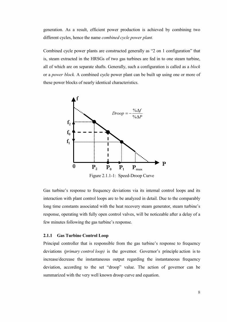
Figure 2.1.1-1: Speed-Droop Curve

Gas turbine’s response to frequency deviations via its internal control loops and its

interaction with plant control loops are to be analyzed in detail. Due to the comparably

long time constants associated with the heat recovery steam generator, steam turbine’s

response, operating with fully open control valves, will be noticeable after a delay of a

few minutes following the gas turbine’s response.

2.1.1 Gas Turbine Control Loop

Principal controller that is responsible from the gas turbine’s response to frequency

deviations (primary control loop) is the governor. Governor’s principle action is to

increase/decrease the instantaneous output regarding the instantaneous frequency

deviation, according to the set “droop” value. The action of governor can be

summarized with the very well known droop curve and equation.

f0

f1

f

P P0

f2

P1 P2 Pmax 0

P

fDroop

∆

∆−=%

%

9

Once the droop value is set to the required value (generally 4-8%), governor controls

the corresponding output change for the instantaneous frequency deviation to be in

accordance with the droop relation or in other words in accordance with the equation

of the above speed-droop line.(Figure 2.1.1-1)

Fundamental control system block diagram of a gas turbine and related control signals

are shown on Figure 2.1.1-2. When steady state conditions are taken into account, say

at nominal grid frequency, steady state load on the machine is determined via the load

reference.

Figure 2.1.1-2: Fundamental gas turbine control system block diagram

During transient conditions of system frequency, even if the load reference is kept

unchanged, error introduced to the governor due to the frequency deviation will result

in a change in the output.

Just to underline, in order for a required increase in load to take place, machine must

not be at its maximum operating limit determined by the temperature controller.

If gas turbine and its control system are perceived as a black-box system, load

reference is the only interference point with an outside system, say, an interacting

controller. This interaction takes place in the form of Raise/Lower pulses.

A detailed modeling for the gas turbine and its control system is carried out in the

following chapter. Moreover, details and variation of the control variables can be

observed in the MATLAB Simulink model that accompanies this thesis study.

Governor

Temperature

Controller

L o w S e l e c t

Gas

Control

Valve

Turbine

Frequency

Droop

Load Reference

(Raise/Lower)

Power

10

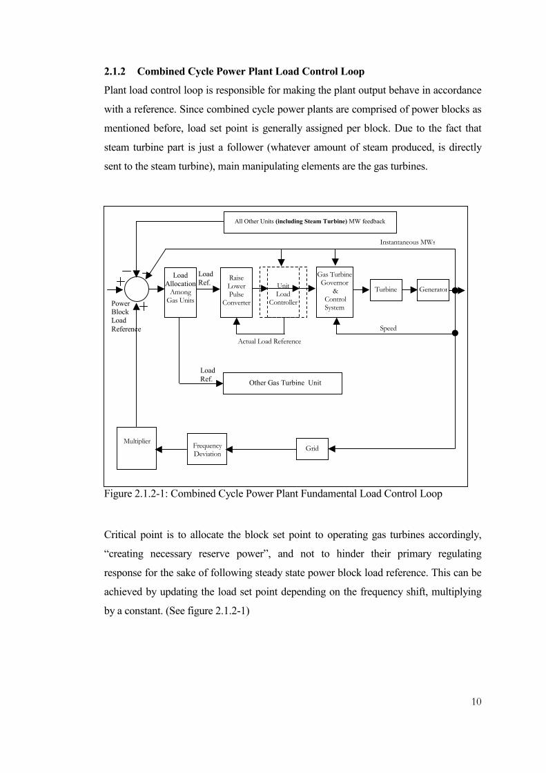
2.1.2 Combined Cycle Power Plant Load Control Loop

Plant load control loop is responsible for making the plant output behave in accordance

with a reference. Since combined cycle power plants are comprised of power blocks as

mentioned before, load set point is generally assigned per block. Due to the fact that

steam turbine part is just a follower (whatever amount of steam produced, is directly

sent to the steam turbine), main manipulating elements are the gas turbines.

Figure 2.1.2-1: Combined Cycle Power Plant Fundamental Load Control Loop

Critical point is to allocate the block set point to operating gas turbines accordingly,

“creating necessary reserve power”, and not to hinder their primary regulating

response for the sake of following steady state power block load reference. This can be

achieved by updating the load set point depending on the frequency shift, multiplying

by a constant. (See figure 2.1.2-1)

Load

Allocation Among Gas Units

Raise Lower Pulse

Converter

Turbine

Gas Turbine Governor &

Control System

Unit Load

Controller

Generator

Load

Ref.

Speed

Instantaneous MWs

Actual Load Reference

Other Gas Turbine Unit

Load

Ref.

All Other Units (including Steam Turbine) MW feedback

Multiplier Frequency Deviation

Grid

Power Block

Load

Reference

11

If load set point for the power block is not updated through the mentioned multiplier,

then closure of total plant/block MW feedback loop will behave in such a way that

instantaneous output changes in response to instantaneous frequency deviations will be

overridden by the plant load controller for the sake of following the steady state load

reference signal.

On Figure 2.1.2-1, symbolic representation of a combined cycle power plant load

control loop is given. See that interfacing to a gas turbine unit by an outside controller

is realized through the application of raise/lower pulses to the load reference input.

Another important point is that “Unit Load Controllers” (detailed discussion on unit

load controllers are given on Chapters 5 and 6) must never be active, otherwise

primary response of the unit is overridden by the unit load controller.

The above depicted control loop was realized in the Simulink model that accompanies

this thesis study.

Reserve power management, although very important and very difficult for gas turbine

based power plants will not be detailed in this study. But modeling approach of this

thesis work offers possible means for controlling reserve power, to be implemented in

“Load Allocation Among Gas Units” block.

12

C HAPTER 3

GAS TURBINE AND CONTROL SYSTEM MODEL

Throughout this chapter, fundamental concerns related to gas turbine units and their

main operating characteristics will be given. Previous studies on gas turbine and

control system modeling will be put forward. Main modeling approach of this thesis

study and methods used will be explained.

3.1 Gas Turbine Basics and Key Differences

Gas turbines and their control systems are significantly different from steam turbine

based power units. One major fact is that their thermal cycle is an “open cycle” using

atmospheric air.

While steam turbines have a closed thermal cycle (steam having been produced in the

boiler, does its work through the turbine and then repressurized back to the boiler

which is a closed volume), in the so called Brayton Cycle of gas turbines, air

compressed through the compressor goes through the combustor and gets burnt with

fuel resulting in high temperature, high pressure exhaust gas. This exhaust gas does its

work while expanding through the turbine (and through the heat recovery steam

generator in combined cycle applications) back to the atmosphere.

This above explained major difference makes maximum power output of the gas

turbine highly dependent on environmental conditions especially to the ambient

temperature and pressure, and determination of this maximum power level is a great

challenge. Another important parameter that affects gas turbine’s maximum

continuous output is the network frequency due to the fact that axial flow compressor

is directly coupled to the shaft of the turbine and airflow changing with the speed

results in a change in the output.[11]

13

So a gas turbine is a complex, multivariable and dynamic system whose modeling

requires intimate study and analysis.

3.2 Modeling the gas turbine

Modeling of gas turbines has been a great concern of the academic environment.

Although these engines were originally designed for aircraft propulsion they are also

widely used in industrial applications for decades especially in power generation area.

Together with their growing usage and increasing number in power systems, analysis

of their dynamic effects, which are very different in nature compared to steam and

hydro units, became one of the most important research subjects of power system

engineers.

Main concerns in power system area that require generation system modeling are

voltage control, power system stability and generation-load unbalance phenomena, that

is, frequency control. So main concern of my modeling approach will be to reach a gas

turbine simulation model that can represent its response to frequency deviations

accurately. This will require a turbine and a governor model but not a generator and

voltage regulator model.

Gas turbine engines used in power generation applications are divided into two

categories namely being aero-derivative and heavy duty. Aeroderivative gas turbines

being derived by modifying aircraft engines are used for small power generation

applications in 10 to 50 MW ranges, whereas heavy-duty gas turbines having different

mechanical construction characteristics are mainly designed for power generation

levels up to 300 MWs. On this thesis study, modeling details of a heavy-duty gas

turbine will be given.

3.2.1 Gas turbine modeling approaches and justification of the approach used.

There are different approaches in gas turbine modeling. First approach is

thermodynamic modeling by using fundamental heat and mass balance equations for

the compressor, combustor and turbine which are the three main components of a gas

turbine engine. Such kind of modeling require going into the deep insides of the

14

machine internal physics (enthalpy equations, efficiency calculations…), especially to

reach accurate steady state and dynamic response characteristics.[9]

The other end of approaches in modeling is the use of generic gas turbine models

subject to some parameter and predetermined function modifications like maximum

power level and frequency dependency of the output. Dynamic effects are included

with simple time constants. Through this approach, a general representation of a gas

turbine unit can be reached. This approach is mostly preferable for system-wide

analysis that will require the models of hundreds of units.[10]

Modeling for power system studies does not require a detailed thermodynamic model

since principal concern is to analyze unit’s dynamic behaviour with respect to

frequency deviations around the main operating point, the nominal grid frequency. So

machines’ internal variables or start-up details, in other words, internal behaviour of

the engine, although might be important for the engine performance studies, are not

required for most power system studies. This does not mean that generic models are

perfectly suitable for all power system analysis purposes. Once reserve power for gas

turbines is under concern, modeling requirements cannot be that much away from

physical principles. Also inclusion of various dynamic effects is a must. That’s why

Rowen’s model [5] and its derivatives [6], [11] which stand in between generic models

[10] and highly detailed thermodynamic models [9] are good starting points for

analysis on gas turbines.

As the modeling approach of this thesis work, static components which reflect the

steady-state input-output relationships of fundamental physical variables were obtained

by some detailed input-output data analysis as a result of the experiments carried out

[3], [11]. For the dynamic characteristics, various papers [5], [6], were analyzed

modified and tuned accordingly to enlarge on the load control loops that are important

for interconnected grid operation.

3.2.2 General physical structure of a gas turbine unit

A gas turbine is comprised of three major components, which are the axial compressor,

combustor(s) and the turbine. Air compressed through the compressor goes through the

15

combustor and gets burnt with input fuel resulting in high temperature, high pressure

exhaust gas. This exhaust gas does its work while expanding through the turbine (and

through the heat recovery steam generator in combined cycle applications) back to the

atmosphere.

Figure 3.2.2-1: Heavy duty gas turbine

Primary input variables are “fuel flow” and “airflow”. Fuel flow is a completely

controllable parameter whereas airflow which is a function of ambient temperature

together with shaft speed (or power system grid frequency) can be regulated with the

help of compressor inlet guide vanes (IGVs) up to a certain degree. Airflow and its

interaction with shaft speed is one of the key points to be solidly understood in gas

turbine operation.

Primary output variables are electrical power from the generator, exhaust temperature

of the turbine (T2) and pressure ratio across the compressor (P1/Patm), all of which

can be measured with no difficulty.

Fuel and air flows are adjusted such that required output power is attained, while

keeping the exhaust temperature (T2) as high as possible taking into account the

maximum permissible turbine inlet temperature (T1).

3.2.3 Gas Turbine Control System

Gas turbine control system is comprised of two important closed control loops namely,

“speed-load controls” and “exhaust temperature controls”. These two control loops are

T2, Patm

HRSG

T1

IGVs &

Compressor G Turbine

Combustion.

Air, Patm

Fuel

P1 P1

16

always in action during operation connected to the grid.

Figure 3.2.3-1 is a block diagram representation of a gas turbine together with its

critical control loops, which is a basis for the simulation model. [5] Overall, as

dynamic elements, there exists simple time constant blocks and transport lags. There

are four fundamental equations that put forward the main thermodynamic

characteristics, which are to be obtained based on input-output data analysis.

3.2.3.1 Governor

On this model, a “droop governor” will be utilized. In large utility systems where the

speed of the turbine is dictated by the grid frequency, droop governor maintains a

proportional action on the error between setpoint, and system frequency. For a detailed

discussion please refer to Chapter 2.

Figure 3.2.3-1: Gas turbine control system

3.2.3.2 Temperature Controller

Temperature controller which is a peculiarity of a gas turbine is the most vital to

understand part of the control system. The main task of the temperature controller is to

limit the fuel flow and/or regulate the airflow (and in turn determine maximum output

together with available reserve power) such that maximum allowable turbine inlet

temperature (T1) is not exceeded in any case. Measurement of turbine inlet

Mechanical

power to the

generator

Governor

Fuel/Air Flow Controls,

actuator

dynamics &

Low Selector

Gas turbine (compressor, turbine and combustion dynamics)

Temperature Controller

Exhaust

Tenp.

Speed

Electrical power

feedback

Fuel flow

Air flow

Load reference

(Raise/Lower)

Speed

deviation.

Speed CPR

Fuel limit

& Part Load IGV

position

17

temperature although possible is not practical due to the temperature levels involved

(approximately 1400 deg C). As a solution, exhaust temperature (T2) is measured and

controlled accordingly at a calculated setpoint, such that firing temperature is kept at

an optimum level.

3.2.3.2.1 Air flow control (Inlet guide vane control)

In combined cycle applications of gas turbines, exhaust temperature is to be kept at

maximum allowable levels even at part load conditions so that optimum performance

on the overall cycle is attained. This can be achieved by closing IGVs under a

controlled manner until exhaust temperature is at maximum allowable level even at

part load.

While IGV control is active, if there is a demand of fuel flow increase, there must be

also a proportional increase in the IGV opening so that temperature limit is not

violated. Temperature Control –IGV- was implemented as a PI controller in the

simulation. (Please refer to Figure D-2 of Appendix D)

3.2.3.2.2 Fuel flow control

Once IGVs are fully open, the machine is on its temperature limit. Further increase on

fuel flow (or further decrease on air flow) must be limited or reversed so that

machine’s internal maximum allowable limit is not offended. This task is achieved by

fuel flow controller of the temperature control system. Temperature Control -Fuel- was

implemented as a PI controller in the simulation. (Please refer to Figure D-2 of

Appendix D)

3.2.3.3 Fuel Control and Combustion System

Fuel control and combustion system consist of fuel control valves, combustors and

volume of the expansion path, all of which introduce a real dynamic characteristic to a

gas turbine unit. [5]

The dominant time constants for fuel control belong to the control valves and storage

volume of the gas piping [5]. There exists a definite time for the combustion to occur

which can be expressed as a transport lag. Once combustion reaction takes place, it

18

takes some time to transport the gas from the combustors through the turbine which is

again to be represented as a transport lag. The continuous displacement of airflow

through the compressor is to be modeled as a simple time constant.[5]

3.2.3.4 Fundamental Equations

Whatever efforts are taken to simplify the mathematical model of the gas turbine, its

inborn thermodynamic characteristics cannot be overlooked in order to reach a

satisfactory model that will mimic the actual behaviour.

Physical principles of the machine are introduced via four fundamental multivariable

“algebraic” equations, which will comprise the “steady-state characteristics” of a gas

turbine unit.

Throughout the modeling process, key point is to reach the structures of the functions

and relationship between independent and dependent variables.

“Slowly varying” input variables and corresponding output data analysis can give

information about steady state characteristics of the machine “free from control system

dynamics”. As a result of purposely slow variation of input variables and based on

above reasoning, the relation between inputs and outputs can be assumed to be

ALGEBRAIC (not dynamic, but static). So, in order to reach the physical equations

that will give information about machine thermodynamics, “curve fitting” approach

can be used on the observed data.

As it can also be seen from gas turbine unit start up and loading data curves in

Appendix A (please see the detailed explanation of each graph), the variables in

concern for each equation and their physical interpretations are as follows.

Output Power (Pout): Output power is a linear function of fuel flow.

)( fout WFP =

Airflow (Wa): Airflow, the most critical equation to be obtained in order to reach other

dependent variables, is a function of speed, Inlet Guide Vane (IGV) position and

19

ambient temperature. Apparent nonlinearity in the speed dependency of airflow can be

observed on Figure A-2, in Appendix A.

),,( aIGVa TNFW θ=

In addition, temperature dependency of airflow must not be ignored. This calls for

similar output data analysis at different temperatures and then temperature dependency

of airflow can be included accordingly.

Compressor Pressure Ratio (CPR): Compressor Pressure Ratio, which is the limiting

factor of maximum output available for the unit and which is used in the exhaust

temperature reference calculation is a function of both airflow and fuel flow. Refer to

Figure A-4 in Appendix A.

),( fa WWFCPR =

Exhaust Temperature (Tx): Exhaust temperature which is the main controlled variable

for the temperature controller is a function of fuel flow and airflow. Refer to Figure A-

5 of Appendix A.

),( afx WWFT =

As it can apparently be seen, airflow equation is the most critical equation to be

reached in order to model the physical characteristics of a gas turbine unit.

To underline once more, the critical point in input-output data analysis and curve

fitting, is to get a function structure that will reflect the physical nature and then reach

the relationship between variables. Following chapter will put forward the data

analysis approach used and how to reach a satisfactory function structure together with

the relationship between variables.

20

C HAPTER 4

EXPERIMENTAL STUDY AND DATA ANALYSIS

Throughout this chapter, data analysis that was carried out to reach four fundamental

equations of the gas turbine simulation model, which were mentioned in the previous

chapter, will be explained. The loading and start-up experiments together with step

response test will be detailed.

“Least Square Regression Analysis” will be carried out on the observed unit start up

and loading data to reach curve fits of what is observed, so that obtained algebraic

equations can be combined with the dynamic model to reflect both dynamic and

steady-state nature of the machine.

Just to underline once more, “slowly varying” input variables and corresponding

output data analysis can give information about steady state characteristics of the

machine “free from control system dynamics”. As a result of purposely slow variation

of input variables and based on this reasoning, the relation between inputs and outputs

can be assumed to be ALGEBRAIC (not dynamic, but static). So, in order to reach the

physical equations that will give information about machine thermodynamics, “curve

fitting” approach can be used on the observed data.

The fundamental relationships to be detailed here are;

• Relationship between output power and fuel flow

• Relationship between airflow, speed, IGV angle and ambient temperature

• Relationship between “compressor pressure ratio”, fuel flow and air flow

• Relationship between exhaust temperature, fuel flow and air flow.

21

4.1 Relationship Between Output Power and Fuel Flow

If we leave aside all the complex and multivariable nature of a gas turbine, it is

basically a device that converts chemical energy of the natural gas to mechanical

energy. Mechanical energy is then converted to electrical energy at the generator.

So, just by intuition, it is easy to say that output power of a gas turbine unit is directly

proportional to input fuel flow but nothing else. The only thing under concern is

whether this relation is linear or not. Closer look to Figure A-1 of Appendix A

indicates an apparent linearity between fuel flow and output power. So the function

structure for this relationship can be proposed to be,

baWP fout += ……………….………………………………...…….(Eqn 4.1-1)

where a and b are the parameters to be determined.

Once data of the linear region of Figure A-1 is transferred to the Matlab for Least

Square Analysis with the proposed function structure of equation 4.1-1, the linear fit

seen on Figure C-1 of Appendix C is obtained.

As it can be seen on Figure C-2, assumption of a linear function like a first order

polynomial results a successful fit of error less than 1% for the analyzed range of

power-fuel flow relationship.

4.2 Relationship between Airflow, Speed, IGV Angle and Temperature

Airflow equation is the most critical function to be reached in order to be able to

calculate the remaining variables of the machine and to establish the proposed gas

turbine model.

Airflow through the machine is created by the compressor coupled to the turbine.

(Refer to Figure 3.2.2-1 in chapter 3.). Simple mechanics tell us that with constant

pressure difference, flow through a restriction is proportional with the area of the

restriction. So IGV angle or in other words, the amount that the inlet guide vanes are

open, has a definite effect on the airflow through the machine. Also, if we are talking

about an axial flow compressor like the case we have on a gas turbine unit, basic

22

mechanics again say that the amount of airflow is directly proportional with the speed

of rotation. Once we also take into account that we are speaking in terms of mass flow

and air is a gas, then temperature is also important for us due to the fact that density of

air changes with temperature resulting a change in total mass flow, although speed and

IGV angle remains constant.

Please refer to Figure A-2 and A-3 in Appendix A. Figure A-2 was obtained during a

unit start-up, i.e. while the unit is brought to 3000 rpm from standstill. On this graph

dependency of airflow both to the speed and IGV angle can be clearly seen. See that

while IGV angle is constant at around 27 degrees, airflow increases with the increasing

speed. When IGV angle changes from 27 to 55 degrees, a very apparent change in

airflow can be observed. Once IGVs were settled at 55 degrees, further increase in

airflow is due to speed only.

Figure A-3 was obtained after synchronization to the grid and while the unit is being

loaded up. The change in speed is only due to random oscillations of the power

network. Also on this graph, apparent dependency of airflow to the IGV angle can be

seen while IGVs are opened up from 55 degrees to 86 degrees.

Being a multivariable function with independent uncontrollable variable speed or

namely the grid frequency and controllable variable IGV angle, it is not an easy task as

the previous power-fuel flow relation to reach a successful fit of the airflow. Also

temperature dependency requires long-term observation while the other parameters are

constant.

4.2.1 A proposal for the function structure of airflow equation

All the above explanation and reasoning prove that airflow is a function of speed, IGV

angle and temperature.

),,( aIGVa TNFW θ= …………………………...….………….(Eqn 4.2.1-1)

The preceding function of several variables can have any structure like division,

multiplication, addition or even square root of the variables under concern. In order to

23

carry out a curve fit, first of all a function structure is necessary. Then necessary

parameters of the determined function structure can be searched through the

minimization of the error.

For example in the case of power-fuel flow fit, being a function of only one variable

and apparent observable linearity could easily let us use a first order polynomial as the

function structure for the fitting process. But in this case, we have a function of many

variables and determining the right function structure that will contain all the variables

while also reflecting the physical reality is not an easy task.

All the data trends that were collected from the machine have some period of time

where only one variable under concern changes while the other is constant. (Please

refer to Figure A-2 and A-3 in Appendix A.) So with this nature of the variables, initial

function structure is considered to be;

)().().(. 321 aIGVa TFFNFKW θ= ……….……………….(Eqn 4.2.1-2)

where K is the scaling constant, F1 is the speed dependency function, F2 is the IGV

opening dependency and F3 is the temperature dependency function for the overall

airflow equation. The next step was then to determine the structure of the functions of

only one variable while keeping the other variable constant and reaching the necessary

equation of airflow.

4.2.2 A closer look to Figures A-2 of Appendix A

It is obvious that we do not have the control of speed once the machine is connected to

the network. But if the machine is separated from the grid, speed of the machine can be

controlled just as it is done during start-up. So the last region of Figure A-2, where

IGV angle is constant at 55 degrees and speed is increasing to 3000 rpm, can be a

beneficial region to find out the speed dependency of airflow. This is useful to

understand the dependency of airflow to severe grid frequency changes during daily

operation.

24

Figure 4.2.2-1 A different look at Figure A-2 for 90-100 % speed range. Airflow vs.

speed and second order polynomial fit.

Figure 4.2.2-1 is obtained by using the data of Figure A-2 for the speed values over

90%. The apparent non-linear relationship between airflow and speed can be readily

seen. The first proposal to this non-linear relation is a second order polynomial as,

edNcNNFWa speed ++==2

1)( )( ……………………..……….(Eqn 4.2.2-1)

Second order polynomial (red line) drawn over the observed data proves to be a

successful fit for the speed function of the airflow equation.

4.2.3 A closer look at Figures A-3 of Appendix A

When the unit is connected to grid and if system frequency does not have significant

oscillations it can be accepted that the speed function of airflow is constant. Then the

change of IGV angle introduced at Figure A-3 will be useful to determine the IGV

opening dependency of airflow.

25

Figure 4.2.2-2 Data of Figure A-3 of Appendix A drawn for IGV angle range of 55 to

86 degrees. Airflow vs. IGV angle and second order polynomial fit.

Figure 4.2.2-2 is obtained by using the data of Figure A-2 for IGV angle range

between 55 and 86 degrees. The non-linear relationship between airflow and IGV

opening can be observed. The first proposal to this non-linear relation can be again a

second order polynomial as,

hgfFWa IGVIGVIGVIGV ++== θθθ2

2)( )( ……….………………………….(Eqn 4.2.3-1)

Second order polynomial (red line) drawn over the observed data proves to be a

successful fit for the IGV angle dependency of the airflow.

4.2.4 Temperature Dependency of Airflow and final Airflow equation

As it was previously mentioned, our main concern is the air mass flow through the

machine and its effects on other variables like temperature. So air being a gas,

26

temperature and also pressure have certain effects on its density, resulting a

considerable effect on the air mass flow.

Unlike other variables, ambient temperature and pressure are totally uncontrollable

variables and have a comparably very slow rate of change. Temperature and pressure

dependency of airflow require very long term observation of unit behaviour while all

the other parameters that affect airflow are constant which is a hard to attain

experimental condition. Hence, previous approach is not applicable.

For this study, pressure dependency of airflow was ignored and it was tried to reach

temperature dependency, through long-term observation of different units at nearly

equal parameters that affect airflow as far as those situations could be caught. That’s

why there is not a parametric way of representing temperature dependency of airflow

in this thesis. Though, intuitively, following equation can be used, knowing the fact

that air mass flow is inversely proportional with temperature since density of air

decreases with increasing temperature.

adesignaTa TCTTFWa /)deg15()(3)( == ……………………………....(Eqn 4.2.4-1)

So the final airflow equation becomes,

adesignIGVIGVa TCThgfedNcNKW /)deg15().).(.(22

++++= θθ .…...(Eqn 4.2.4-2)

Figure C-3 in Appendix C contains both the airflow data of Figure A-3 of Appendix A

and obtained fit on the same graph together with error analysis.

4.3 Relationship between “compressor pressure ratio”, fuel flow and air flow

Again let’s have a closer look at Figure 3.2.2-1 of Chapter 3. Basically what the

compressor does is, maintaining continuous airflow by supplying compressed air to the

combustor which is necessary for the combustion to take place. The more compressed

air provided for the combustion, the more fuel can be input and in the end, more power

can be produced. But just like every machine a gas turbine unit has certain limits and

27

measurement of pressure ratio across the compressor is necessary to determine and not

to offend those limits.

In the end, the philosophy of gas turbine control is to keep the turbine inlet temperature

(T1) at its limit despite the fact that it cannot be measured. Measuring exhaust

temperature, which is at acceptable levels, together with the compressor pressure ratio,

one can calculate turbine inlet temperature and do not offend the limit.

Please refer to Figure A-4 of Appendix A. See that there is a period of time where fuel

flow changes but air flow is constant. There is also a longer period of time where both

air and fuel flows change. It is apparently seen that compressor pressure ratio increases

at a certain rate with the increase of fuel flow but this rate goes higher in the region

where both fuel and air flows increase together. So it is obvious to say that compressor

pressure ratio is a function of both fuel and air flows.

While curve fitting, in order to benefit from the region where fuel flow changes only,

with the same reasoning that was used for airflow equation, it can be assumed that,

)().(),( 21 afaf WFWFWWFCPR == ……………………………………....(Eqn 4.3-1)

Next step becomes to reach F1(Wf), in the region where airflow is constant. As,

)(. 1 fWFKCPR = ……………….………………...……………………….(Eqn 4.3-2)

Then using the mathematical fact that,

)()(

2

1

a

f

WFWF

CPR= ………………..……………………………………(Eqn 4.3-3)

F2(Wa) is the curve fit to reach for the data values obtained as a result of the division.

CPR is measured and F1(Wf) is obtained in the preceding step.

28

Figure 4.3.1 Curve fit to data of Figure A-4 of Appendix A for the period where

airflow is constant. F1(Wf) is obtained as a result of the fit.

As a result CPR equation can be reached with the multiplication of F1 and F2. Please

take a look at to linear fits obtained for F1(Wf) and F2(Wa) on figures 4.3.1 and 4.3.2.

Final CPR equation becomes as,

)).(()().( 21 nmWlkWWFWFCPR afaf ++== …………………….……..(Eqn 4.3-4)

Please see Figure C-4 of Appendix C for the overall CPR fit and corresponding error

analysis.

29

Figure 4.3.2: F2(Wa) is obtained as a result of the linear fit obtained for the

CPR/F1(Wf) vs. Airflow data. See that data values below 0.82 of airflow were

intentionally excluded from the fit. This is to increase accuracy at higher air and fuel

flow operation region i.e. higher MW operating point where we operate the machine

normally.

4.4 Relationship between exhaust temperature, fuel flow and air flow

Another glance at Figure 3.2.2-1 of Chapter 3 might be helpful to understand what is

mentioned by the exhaust temperature (T2).

Measurement of exhaust temperature is the controlling means of a gas turbine unit

since the main variable to be kept under a limit, that is, turbine inlet temperature (T1)

cannot be measured.

It is easy to accept that exhaust temperature is dependent on two factors that are air

flow and fuel flow, this apparent dependency can also be observed by looking at

Figure A-5 of Appendix A. See that there is a period of time where air flow is constant

but fuel flow is increasing accompanied with a corresponding increase on the exhaust

30

temperature. After a certain temperature value, increase in airflow together with an

increase in fuel flow results in a decrease at exhaust temperature.

With the same reasoning that was followed at the preceding curve fit trials e.g. CPR

equation, in order to benefit from the region where airflow is constant but fuel flow is

changing, the relationship can be established as;

)().(),( 21 afafx WFWFWWFT == ……………….………………….……..(Eqn 4.4-1)

Next step becomes to reach F1(Wf), in the region where airflow is constant. As,

)(. 1 fx WFKT = ………………….………………………...…………...(Eqn 4.4-2)

then using the fact, just like it was used for reaching the CPR equation,

)()(

2

1

a

f

x WFWF

T= …………………..……………………………………(Eqn 4.4-3)

where F2(Wa) is the curve fit to reach for the data values obtained as a result of the

division. Tx is measured and F1(Wf) is obtained in the preceding step.

As a result exhaust temperature equation can be reached with the multiplication of F1

and F2. Please take a look at to linear fits obtained for F1(Wf) and F2(Wa) on figures

4.4.1 and 4.4.2.

Final exhaust temperature becomes,

)).(()().( 21 srWqpWWFWFT afafx ++== …….………….……………(Eqn 4.4-4)

Please see Figure C-5 of Appendix C for the overall exhaust temperature fit and

corresponding error analysis.

Consequently, all the critical variables of a gas turbine unit are reached for the

simulation.

31

Figure 4.4.1: Curve fit of measured exhaust temperature to measured fuel flow when

airflow is constant. F1(Wf) of equation 4.4.2 is obtained as a result of the fit.

Figure 4.4.2: Curve fit of Tx/F1(Wf) obtained in the preceding step to measured

airflow data. As a result F2(Wa) is obtained as a linear fit.………………..

32

C HAPTER 5

SIMULATION MODEL

Plant load control system for a combined cycle power plant, proposed in Chapter 2

was realized as a MATLAB Simulink model, details of which will be given in this

section. Applied simulation model can be seen in Figure D-1 of Appendix D.

Proposed model consists of two dynamic gas turbine models, a simple dynamic steam

turbine model and a plant load controller model.

The steady state characteristics and fundamental variables of the gas turbine model

were obtained as a result of experimental studies and curve fits detailed in Chapter 4.

For the dynamic model, as the starting point, the “structure” provided by Rowen of

General Electric [5], [6] was used. As both of those models are for some other specific

applications, in order to reflect the dynamic nature called for this study, that is, power

system frequency control point of view, modifications were carried out in the model

structure. A “load controller” for the gas turbine unit was also integrated to the model.

Applied gas turbine simulation model in block diagram configuration can be seen in

Figure D-2 of Appendix D.

Steam turbine was modeled as the cascade combination of steady-state characteristics

obtained as a result of “gas turbine power” to “steam turbine power” curve fit and

apparent dynamics. For simplicity, steam turbine dynamics were just introduced as a

single “time delay” element. Justification of this approach is straightforward. By

experience, it is common practice to operate combined cycle power plants close to

their maximum operating point. So at this stage, whatever steam produced at the

HRSGs (Heat Recovery Steam Generator) of the gas turbines, are let through the fully

open control valves of the steam turbine. That’s, basically there is no dynamic control

33

at the steam turbine when it is operating under this “sliding pressure control mode”. In

sliding pressure control mode, whatever steam delivered to the steam turbine is let

through without any active control at the valves by neither the governor nor the

pressure controller. This is actually the turbine-follow mode [3].

Plant load controller is the interfacing means to the gas turbine units. Load reference to

be followed by the power block is introduced only to the gas turbine units, since steam

turbine is just a follower. As it was also mentioned in Chapter 3 while detailing on the

gas turbine control system, interfacing to the gas turbine can be via raise/lower pulses

to the load reference. So conversion of analog set point to raise/lower pulses together

with required control system dynamics are carried out on this block.

To underline once more, in case of an “analog set point” but not raise/lower pulses sent

to the power block, total plant load control loop must be closed to follow up the

reference. When total plant/block MW feedback loop is closed, instantaneous output

changes in response to instantaneous frequency deviations will create an error for the

plant load controller if its input is a steady state reference signal. Then this error is to

be eliminated by the plant load controller for the sake of following reference signal,

“which means hindering the primary response”.

Gain “K” (please refer to Figure D-1of Appendix D) that acts on frequency error and

adds up to the load reference, updates the set point as long as there is a frequency

deviation. As a result, instantaneous megawatt output change is not considered as an

error by the plant load controller having a steady state load reference.

5.1 Gas Turbine Big Block

Gas turbine big block expects a load control set point when load controller of this

specific unit is activated via “1” through the “Activate Load Controller” input.

When load controller of the specific unit is not activated and “plant load controller” is

active, raise/lower pulses that increment/decrement the load reference are input

through the “Raise/Lower Pulses from Plant Control” input.

34

The speed or “frequency” information for the governor and airflow calculation model

is applied to the corresponding input.

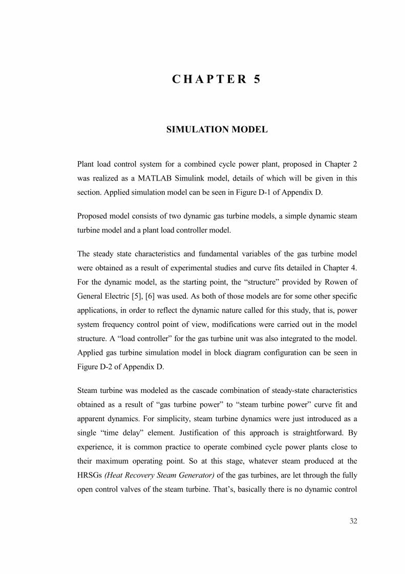
Figure 5.1: Gas turbine big block of the simulation model

“Instantaneous Power” is the output power in megawatts. “Load Reference” is an

internal variable but used as a feedback signal to the “Plant Load Controller”

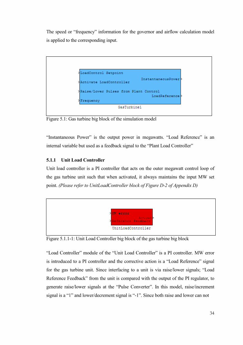
5.1.1 Unit Load Controller

Unit load controller is a PI controller that acts on the outer megawatt control loop of

the gas turbine unit such that when activated, it always maintains the input MW set

point. (Please refer to UnitLoadController block of Figure D-2 of Appendix D)

Figure 5.1.1-1: Unit Load Controller big block of the gas turbine big block

“Load Controller” module of the “Unit Load Controller” is a PI controller. MW error

is introduced to a PI controller and the corrective action is a “Load Reference” signal

for the gas turbine unit. Since interfacing to a unit is via raise/lower signals; “Load

Reference Feedback” from the unit is compared with the output of the PI regulator, to

generate raise/lower signals at the “Pulse Converter”. In this model, raise/increment

signal is a “1” and lower/decrement signal is “-1”. Since both raise and lower can not

35

Figure 5.1.1-2: Building blocks of the Unit Load Controller

be active at the same time, appropriate integration of those raise/lower signals at the

“PulsetoRefConverter” block give the total amount of change to be made on the load

reference.

Figure 5.1.1-3: Building blocks of the PulseConverter

For the discussion of other internal blocks used in this gas turbine big block, please

refer to Figure D-2 of Appendix D and detailed information given in Chapters 3 and 4.

36

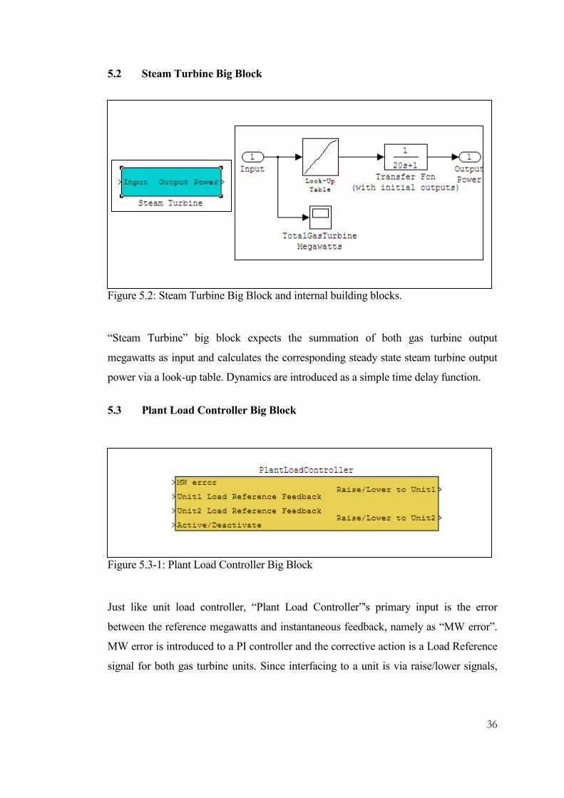
5.2 Steam Turbine Big Block

Figure 5.2: Steam Turbine Big Block and internal building blocks.

“Steam Turbine” big block expects the summation of both gas turbine output

megawatts as input and calculates the corresponding steady state steam turbine output

power via a look-up table. Dynamics are introduced as a simple time delay function.

5.3 Plant Load Controller Big Block

Figure 5.3-1: Plant Load Controller Big Block

Just like unit load controller, “Plant Load Controller”'s primary input is the error

between the reference megawatts and instantaneous feedback, namely as “MW error”.

MW error is introduced to a PI controller and the corrective action is a Load Reference

signal for both gas turbine units. Since interfacing to a unit is via raise/lower signals,

37

“Load Reference Feedback” from the units is compared with the output of the PI

regulator, to generate raise/lower signals at the “Pulse Converter” same as used in Unit

Load Controller. Similarly integration of those raise/lower signals gives the total

amount of change to be made on the load reference.

Figure 5.3-2: Building blocks of the PlantLoadController big block

38

C HAPTER 6

SIMULATION RESULTS AND DISCUSSION

6.1 Primary Response of a Gas Turbine Unit to a Frequency Deviation

Let us assume that the gas turbine unit whose primary response will be simulated here

is a 250 MW rated output machine and has 5% governor droop characteristic.

When we analyze the case of gas turbine units that have droop governors and are

connected to a large interconnected system, participation of one or two units to a

frequency deviation by changing their output, can not make the system reach an

equilibrium point but can only play a minor role to reach the mentioned equilibrium.

Only the contribution of many units can make the system reach a quasi-steady state

equilibrium in an interconnected network.

For the purpose of this study, in analyzing the response of a gas turbine and a

combined cycle power plant’s response to a frequency change; quasi-steady state

deviation in the frequency will be a controllable disturbance that is intentionally

introduced and removed to the frequency or speed inputs of the turbines. So the grid

behaviour, which can only be represented by the collection of many power plants will

be “assumed” to be a frequency disturbance that can be manipulated on, just for the

ease of applicability. In the end whatever the response of the unit that is being

simulated, grid will behave with its own distributed characteristic, which can only be

assumed to be in accordance with our desires for the simulation case of a power block

of a combined cycle power plant.

39

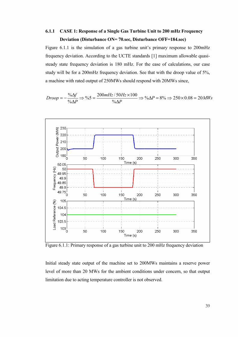
6.1.1 CASE 1: Response of a Single Gas Turbine Unit to 200 mHz Frequency

Deviation (Disturbance ON= 70.sec, Disturbance OFF=184.sec)

Figure 6.1.1 is the simulation of a gas turbine unit’s primary response to 200mHz

frequency deviation. According to the UCTE standards [1] maximum allowable quasi-

steady state frequency deviation is 180 mHz. For the ease of calculations, our case

study will be for a 200mHz frequency deviation. See that with the droop value of 5%,

a machine with rated output of 250MWs should respond with 20MWs since,

MWsPP

HzmHz

P

fDroop 2008.0250%8%

%

10050/2005%

%

%=×⇒=∆⇒

∆

×=⇒

∆

∆−=

Figure 6.1.1: Primary response of a gas turbine unit to 200 mHz frequency deviation

Initial steady state output of the machine set to 200MWs maintains a reserve power

level of more than 20 MWs for the ambient conditions under concern, so that output

limitation due to acting temperature controller is not observed.

40

Please see that machine responds to the frequency deviation naturally without any

interference to the “steady state load reference” (%Load reference is constant at %104

through the simulation period as on Figure 6.1-1. Signal depicted as Point “A”on

Figure D-2 of Appendix D.). Hence, when frequency deviation is over, machine is

back at its initial, steady state operating point.

Figure 6.1.2-1: Primary response of a gas turbine unit to 500 mHz frequency deviation.

6.1.2 CASE 2: Response of a Single Gas Turbine Unit to 500 mHz Frequency

Deviation (Tambient=T, Disturbance ON=70.sec, Disturbance OFF=190.sec)

As any other machine, a gas turbine unit also has a maximum output controlled by the

temperature controller. (Temperature Control -Fuel- on Figure D-2 of Appendix D).

Peculiarity of the gas turbine unit is the dependency of this maximum output to many

factors, especially to the ambient temperature. 500 mHz deviation in the frequency will

force the machine to reach its maximum output as a result of its primary response. On

Figure 6.1.2-1, output power limitation due to acting temperature controller can be

41

seen. Although, governor increases the output to 250 MWs, required for 500mHz

frequency deviation, temperature controller pulls back the output to the maximum

allowable operating point that machine can withstand continuously at these ambient

conditions. Please refer to Figure 6.1.2-2 where fuel flow reference from the governor

and fuel flow reference from the temperature controller can be observed (signals

depicted as “B” and “C” respectively on Figure D-2 of Appendix D). Once the fuel

flow reference signal from the Temperature Controller is less than the fuel flow signal

generated by the Governor, it passes through the “minimum value selector” and

applied to the gas control valves.

Figure 6.1.2-2: Fuel flow reference signals both from governor and temperature

controller. See that, while governor increases the fuel reference in order to respond to

frequency deviation, temperature controller decreases its output. The lower value

becomes valid due to the minimum value selector.

42

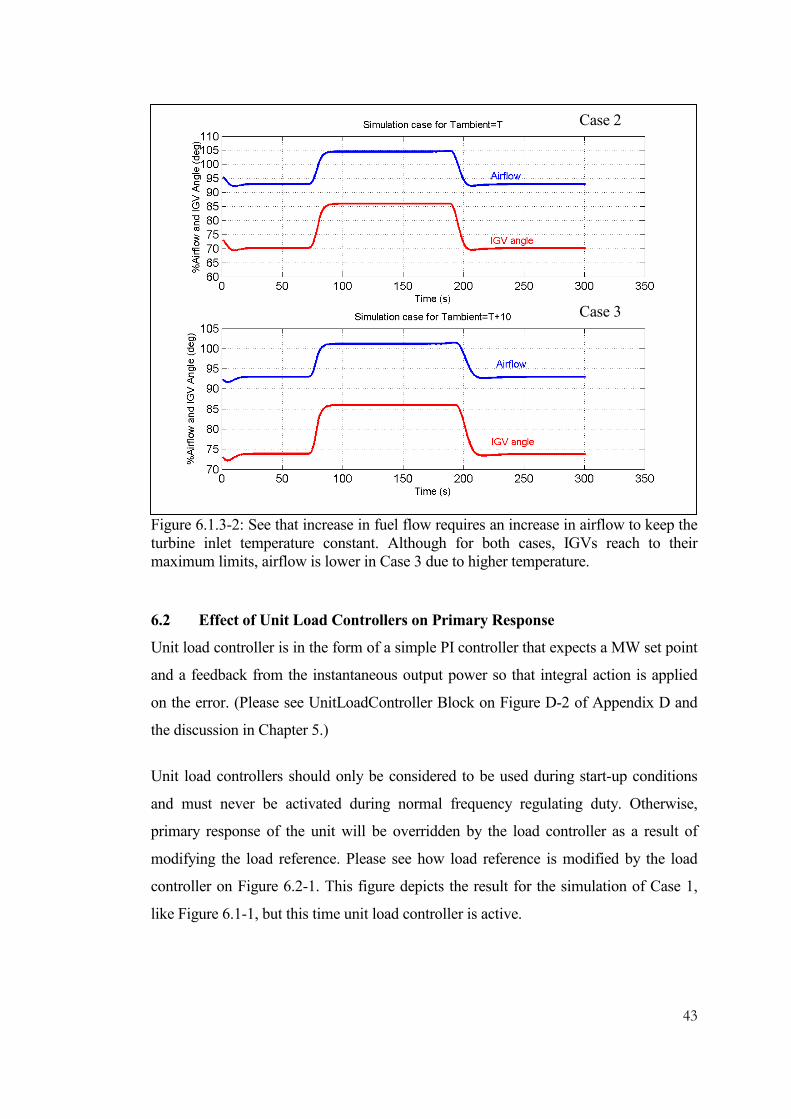
6.1.3 CASE 3: Response of a Single Gas Turbine Unit to 500 mHz Frequency

Deviation (Tambient=T+10, Disturbance ON=70.sec, Disturbance OFF=

190.sec)

This simulation case is identical with the preceding case except that ambient

temperature was taken 10 degrees higher. Please see on Figure 6.1.3-1 that the

maximum allowable point is much lower, due to the fact that increase in temperature

will result in reduced airflow through the machine.

Figure 6.1.3-2 summarizes the simulation of the IGV angle (signal “D” of Figure D-2

of Appendix D) and corresponding airflow change (signal “E” of Figure D-2) for Case

2 and Case 3, where Tambient=T and Tambient=T+10 respectively.

Figure 6.1.3-1: Primary response of a gas turbine unit to 500 mHz frequency deviation.

Please see that due to higher ambient temperature unit cannot respond with the same

reserve power as it provided for the preceding case.

43

Figure 6.1.3-2: See that increase in fuel flow requires an increase in airflow to keep the

turbine inlet temperature constant. Although for both cases, IGVs reach to their

maximum limits, airflow is lower in Case 3 due to higher temperature.

6.2 Effect of Unit Load Controllers on Primary Response

Unit load controller is in the form of a simple PI controller that expects a MW set point

and a feedback from the instantaneous output power so that integral action is applied

on the error. (Please see UnitLoadController Block on Figure D-2 of Appendix D and

the discussion in Chapter 5.)

Unit load controllers should only be considered to be used during start-up conditions

and must never be activated during normal frequency regulating duty. Otherwise,

primary response of the unit will be overridden by the load controller as a result of

modifying the load reference. Please see how load reference is modified by the load

controller on Figure 6.2-1. This figure depicts the result for the simulation of Case 1,

like Figure 6.1-1, but this time unit load controller is active.

Case 2

Case 3

44

Figure 6.2-1: Simulation of a gas turbine unit’s primary response to frequency

deviation when unit load controller is active with a set point of 200MWs.

First of all see that initial transient in the output is just because of the initialization of

the model. Primary response expected to be seen on Figure 6.1-1 is overridden by the

acting unit load controller, which is strictly not desired for normal operation.

Explanation of the major difference on the above figure is straightforward. Please refer

to Figure D-2 of Appendix D. Once there is a frequency deviation, an error is

generated to be zeroed by the governor since it is a PI controller. Output of the

governor is transferred to the gas control valves, resulting an increase in fuel flow

(signal “G”) to the turbine and in turn increase in MWs. (signal “H”) Power being

filtered and scaled, is fed back to the governor so that error for the governor is

eliminated. It is also fedback directly to Unit Load Controller. If unit load controller is

active, output (signal “H”) being different than steady state MW set point (signal “J”)

of the load controller will introduce a non-zero error (signal “K”), which will in turn

introduce non-zero controlling action (signal “L”) on the load reference (signal “A”).

45

As can be seen on Figure 6.2-1, contrary to preceding cases, even when the frequency

is at temporary equilibrium with a certain deviation from initial steady state, output

power of the unit is maintained again at 200MWs by modifying the load reference.

6.3 Primary Response of a Power Plant Following an External Plant Load

Reference Signal

In the end, a power plant is a collection of generating units and it is natural to expect

that the same behaviour will be observed on a larger scale. The main point here is, to

implement the required interfacing system so that expected plant behaviour can be

achieved.

Figure 6.3-1: If a load reference signal which is not updated accordingly to be

considered as an instantaneous reference signal is introduced to the system as if it were

an instantaneous reference signal, then primary response of the power plant will be

overridden.

Figure 6.3-1 is the behaviour of a power block to a 200 mHz frequency drop, without

an external droop characteristic for the whole block being implemented. In the figure

46

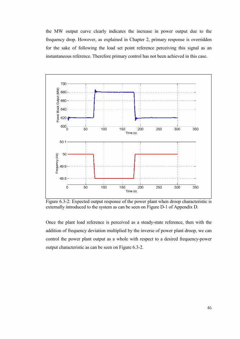
the MW output curve clearly indicates the increase in power output due to the

frequency drop. However, as explained in Chapter 2, primary response is overridden

for the sake of following the load set point reference perceiving this signal as an

instantaneous reference. Therefore primary control has not been achieved in this case.

Figure 6.3-2: Expected output response of the power plant when droop characteristic is

externally introduced to the system as can be seen on Figure D-1 of Appendix D.

Once the plant load reference is perceived as a steady-state reference, then with the

addition of frequency deviation multiplied by the inverse of power plant droop, we can

control the power plant output as a whole with respect to a desired frequency-power

output characteristic as can be seen on Figure 6.3-2.

47

C HAPTER 7

CONCLUSION

In this thesis, load frequency control model for a combined cycle power plant is

analyzed and a simulator is developed to investigate the behaviour of the power plant

under various disturbances.

Principle building blocks of combined cycle power plants are the gas turbines. Due to

this fact, a gas turbine model that will also include the physical nature of the machine

was obtained in this study. As the modeling approach, static components that reflect

the steady-state input-output relationships of fundamental physical variables were

reached by curve fitting to the input-output data collected through the experiments

performed [11]. For the dynamic characteristics, various papers [5], [6], were

analyzed, modified and tuned accordingly to enlarge on the load control loops that are

important for interconnected grid operation.

Generating units in a power plant, which are nominated to participate in system

frequency control must not be at their maximum operating point (base load), but must

be operated under “governor control” with certain, predetermined amount of reserve

power. Of course in addition to these facts, proper control over correctly configured

load control loops is a must. Otherwise, units will either not respond to frequency

deviations or; those respond, will have to load/unload in large magnitudes to an extent,

frequency occurrences of which might not only worn out the machines but also result

in inadvertent grid behaviour. So appropriate control loop implementation is a must for

all power plants.

48

Reserve power control, although very important and very difficult for gas turbine

based power plants was not analyzed in this study. But modeling approach of this

thesis work offers possible means for controlling reserve power at gas turbines so that

predetermined amount of frequency responsive reserve power can continuously be

maintained.

Regarding the testing work done on the gas turbines, step change tests in speed

feedback of the turbine governors can only give information on the droop value and

loading rates of those machines. Such kind of tests will not and cannot give “definite”

information about performance of reserve power provision.

Primary reasoning for the above claim is that frequency and in turn air flow which is

critical for the temperature limiter does not actually change during such a test;

secondly those tests are carried out at “test” conditions of vast reserve power levels at

which machines are hardly operated. So success on those tests does not have to reflect

the reality. That’s why, “15 minutes of continuous operation at the quasi-steady state

frequency requirement of UCTE” [1] must be understood in terms of above claim

especially for gas turbines, because hydro and steam units do not have the previously

explained characteristic of the gas turbines.

There is one more concept that needs to be clarified in the evaluation of primary

control response. Turbine rotors of 40 to 60 tons of 3000 rpm rotating masses are huge

kinetic energy reservoirs with their high inertias. So instant and short load pickups (1

to 3 seconds of 2-4 MWs at falling frequency) are purely because of the inertial

response and cannot be continuously maintained without increasing the power

generation.

Analysis of Turkey’s grid frequency (please refer to Figure E-1 of Appendix E) reveals

the fact that there are continuous oscillations on the frequency even though there is no

major disturbance in the system. One of the key reasons for this apparent problem

might be the primary response being overridden by the inappropriately acting load

controllers or improperly configured power plant secondary control interfaces.

49

Recently, units with digital controllers and that have a Remote Terminal Unit (RTU) at

their sites, are controlled on secondary control by the transmission system operator. It

must not be forgotten that understanding of the reference signal sent to the plant is of

utmost importance. It can either be perceived as a “steady-state reference” signal or an

“instantaneous reference” signal. Correct interpretation of this signal has to be

established among transmission system operator and power plant crew. In any case,

units must be free to utilize their reserve power for the primary response. If a solid

understanding on this issue is not reached, interconnected system’s overall frequency

behaviour can not be improved. Units under the effect of secondary controller’s outer

megawatt control loop, if not controlled correctly, once having given their governor

response to a frequency deviation, will have to respond in an opposite way due to

slowly acting secondary controller. A solution to this problem was presented and

proved in a simulation program in this thesis.

A system-wide simulation, that will not only include the certain dynamic effects of

different power plant types but also the electrical characteristics of generators and

transmission system is probably the best next step to move forward following this

thesis. Once also the AGC algorithm is integrated to this simulation, underlying

principles to have an accurate control on Turkey’s grid frequency can be established.

But it must never be forgotten that, thorough understanding of power plant control

loops is the fundamental concern to achieve a satisfactory solution.

50

R E F ERENCE S

[1] “UCTE Operation Handbook”, Union for the Coordination of Transmission of

Electricity, June 2004.

[2] John Undrill, “Power Plant Operational Issues Relating to Grid Operation”, IEEE

Power Engineering Society General Meeting, 2004.

[3] John Undrill, Garmendia, A., “Modeling of Combined Cycle Plants in Grid

Simulation Studies”, IEEE Power Engineering Society Winter Meeting, vol. 2, pp 657-

663, 2001

[4] John Undrill “Issues of Power Plant Control in relation to System Frequency

Control”, Proceedings of IEEE Winter Power Meeting, pp. 600-603, 1999

[5] W.I.Rowen, “Simplified Mathematical Representations of Heavy-Duty Gas

Turbines”, Trans. Amer. Soc. Mech. Eng., vol.105, pp.865-869, Oct 1983.

[6] W.I.Rowen, “Simplified Mathematical Representations of Single Shaft Gas

Turbines in Mechanical Drive Service” Turbomach. Int., pp. 26-32, Jul./Aug. 1992.

[7] W.I. Rowen, “Dynamic Response Characteristics of Heavy Duty Gas Turbines and

Combined Cycle Systems in Frequency Regulating Duty”, IEE Colloquium on

Frequency Control Capability of Generating Plant, 1995

[8] IEEE Working Group on Prime Mover and Energy Supply Models for System

Dynamic Performance Studies, “Dynamic Models for Combined Cycle Plants in

Power System Studies”, IEEE Transactions on Power Systems, Vol 9, No.3, August

1994

[9] A. Bagnasco, B. Delfino, G.B. Denegri, and S. Massucco, “Management and

Dynamic Performances of Combined Cycle Power Plants During Parallel and

Islanding Operation,” IEEE Trans. Energy Convers., vol 13. no.2 pp. 194-201, Jun.

1998.

51

[10] L.Pereira, J. Undrill, D. Kosterev, D. Davies, S. Patterson, "A New Thermal

Governing Approach in the WECC", IEEE Transactions on Power Systems, Vol. 18,

pp 819-829, 2003.

[11] K. Kunitomi, A, Kurita, H. Okamoto, Y. Tada, S. Ihara, P. Pourbeik, W.W Price,

A.B. Leirbukt, and J.J Sanchez-Gasca, “Modeling Frequency Dependency of Gas

Turbine Output” in Proc. IEEE Power Eng. Soc, Winter Meeting, vol. 2, pp 678-683,

2001.

[12] Kakimoto, Baba, “Performance of Gas Turbine-Based Plants During Frequency

Drops”, IEEE Transactions on Power Systems, vol. 18, pp 1110-1115, 2003

[13] Nagpal, M.; Moshref, A.; Morison, G.K.; Kundur, P, “Experience with Testing

and Modeling of Gas Turbines”, IEEE Power Engineering Society Winter Meeting,

vol. 2, pp 652-656, 2001

[14] L.Hannet, J.W. Feltes, “Testing and Model Validation for Combined-Cycle Power

Plants”, IEEE Power Engineering Society Winter Meeting, vol. 2, pp 664-670, 2001

[15] Berube, Hajagos, “Modeling Based on Field Tests of Turbine/Governor Systems”,

Proceedings of IEEE Winter Power Meeting, pp. 567-573, 1999

52

A P P END I X A

GAS TURBINE UNIT START-UP AND LOADING DATA

SAMPLED AT 4 SAMPLES/SECOND

Figure A-1: Gas turbine unit output and fuel flow relation real time plot with respect to

time. (860 seconds total observation time, 4 samples/sec)

This trend was obtained while loading the unit up. Linear relationship between output

power and fuel flow can be clearly seen.

280 MW, 20 kg/s

0 MW, 4 kg/s

53

Figure A-2: Gas turbine unit start-up real time plot (0 to 100% speed). Dependency of

airflow to speed and IGV (Inlet Guide Vane) position. (1802 seconds total observation

time, 4 samples/sec)

This trend was obtained during a unit start-up ie. while the unit is brought to 3000 rpm

from standstill. Dependency of airflow both to the speed and IGV angle can be

apparently seen. See that while IGV angle is constant at around 27 degrees, airflow

increases with the increasing speed. When IGV angle changes from 27 to 55 degrees, a

very apparent change in airflow can be observed. Once IGVs are settled at 55 degrees,

further increase in airflow is due to speed only.

IGV Angle

Air flow

Speed

120%,100 deg, 500 kg/s

0

54

Figure A-3: Dependency of air flow to IGV angle at constant speed. (647 seconds total

observation time, 4 samples/sec)

This trend was obtained after synchronization to the grid and while the unit is being

loaded up. The change in speed is only due to random oscillations of the power

network. Also on this graph, apparent dependency of airflow to the IGV angle can be

seen while IGVs are opened up from 55 degrees to 86 degrees.

Speed

IGV Angle

Air flow

110%, 100 deg, 700 kg/s

90%, 0 deg, 0 kg/s

55

Figure A-4: Dependency of Compressor Pressure Ratio, to airflow and fuel flow. (840

seconds observation time, 4 samples/sec)

This trend was obtained while the unit is being loaded up. Increase in fuel flow proves

this fact. While loading up, after a certain limit, control system increases airflow to

compensate for the temperature increase that will result due to increasing fuel flow. As

a result, apparent dependency of compressor pressure ratio both to air and fuel flows is

observed.

Compressor Pressure Ratio

Fuel Flow

Air Flow

10 prs_R, 30%, 300 kg/s

18 prs_R, 80%, 800 kg/s

56

Figure A-5: Dependency of exhaust temperature to airflow and fuel flow. (842 seconds

total observation time, 4 samples/sec)

This trend was also obtained during a unit load-up. See that there is a period of time

where air fuel flow is constant but fuel flow is increasing accompanied with a

corresponding increase on the exhaust temperature. After a certain temperature value,

increase in airflow together with an increase in fuel flow results in a decrease at the

exhaust temperature. Hence proving the fact that exhaust temperature is directly

proportional with fuel flow and inversely proportional with airflow.

Air flow

Fuel flow

Exhaust Temp

400 degC, 300 kg/s, 5kg/s

700 degC, 700 kg/s, 25kg/s

57

A P P END I X B

STEP RESPONSE TEST

Figure B-1: Step response of a gas turbine unit to 0.4% change in the load reference.

(133 seconds total observation time, 16 samples/sec )

Load reference

Output

Control Valve_1 % open

Control Valve_2 % open

101 %, 150 MW, 10 %, 60%

105 %, 240 MW, 45 %, 110%

58

AP PEND I X C

OBTAINED CURVE FITS FOR THE OBSERVED

INPUT-OUTPUT DATA

Figure C-1: Output power vs. fuel flow relation. Apparent linearity between fuel flow

and output power together with the first order polynomial fit can be observed.

59

Figure C-2: Analysis of the actual data and the fit for the output power- fuel flow

relationship. Error less than %1 can be accepted as a successful fit.

60

Figure C-3: Analysis of actual data and the fit for the Airflow Calculation.

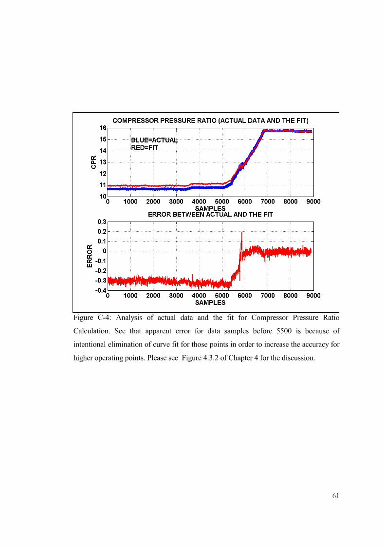
61

Figure C-4: Analysis of actual data and the fit for Compressor Pressure Ratio

Calculation. See that apparent error for data samples before 5500 is because of

intentional elimination of curve fit for those points in order to increase the accuracy for

higher operating points. Please see Figure 4.3.2 of Chapter 4 for the discussion.

62

Figure C-5: Analysis of actual data and the fit for Exhaust Temperature Calculation.

63

A P P END I X D

SIMULATION BLOCK DIAGRAMS

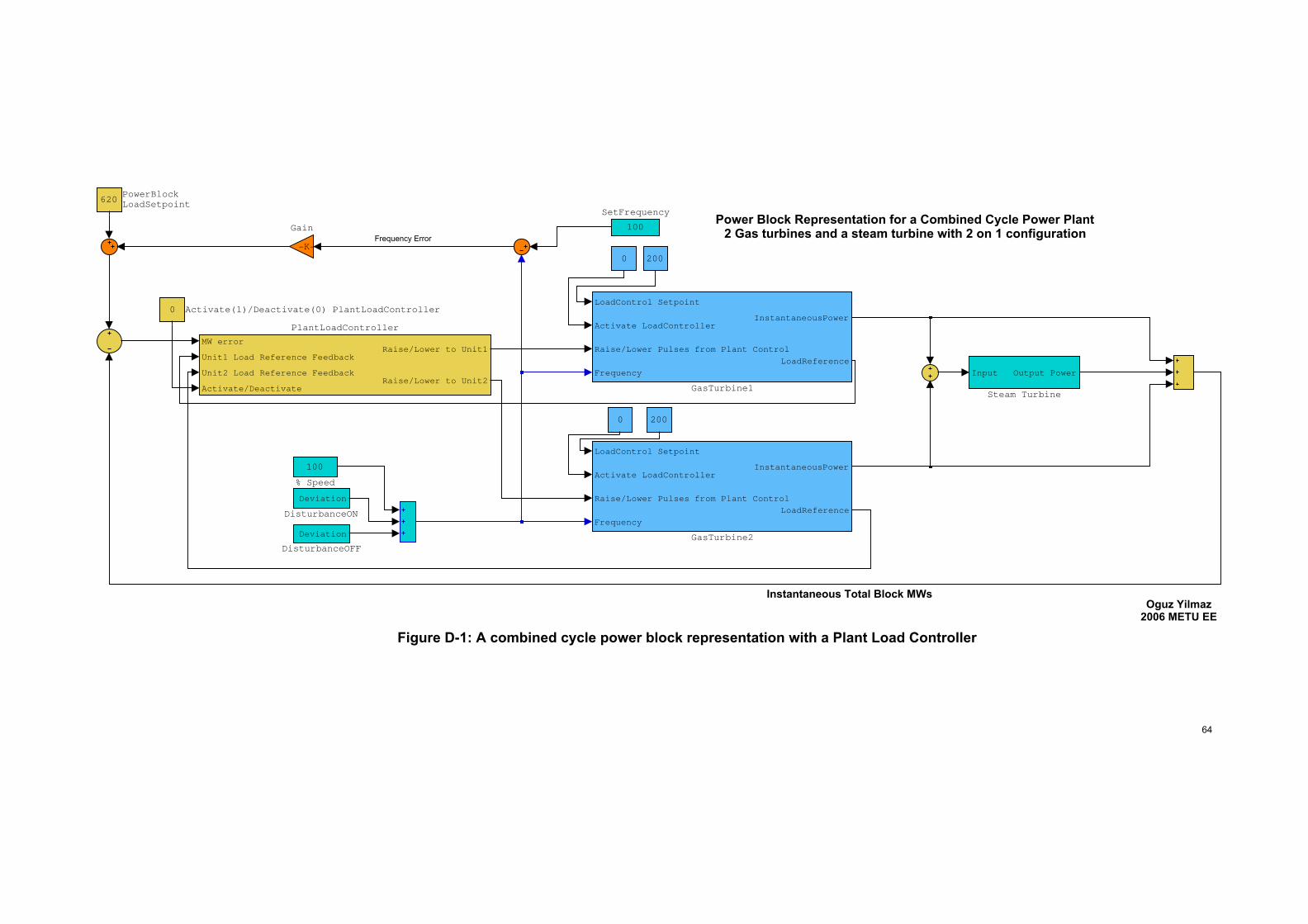
Power Block Representation for a Combined Cycle Power Plant2 Gas turbines and a steam turbine with 2 on 1 configuration

Instantaneous Total Block MWs

Frequency Error

Oguz Yilmaz2006 METU EE

Figure D-1: A combined cycle power block representation with a Plant Load Controller

64

aaa

Oguz Yilmaz2006 METU EE

Oguz Yilmaz2006 METU EE

Input Output Power

Steam Turbine

100

SetFrequency

620PowerBlock

LoadSetpoint

MW error

Unit1 Load Reference Feedback

Unit2 Load Reference Feedback

Activate/Deactivate

Raise/Lower to Unit1

Raise/Lower to Unit2

PlantLoadController

200

200

LoadControl Setpoint

Activate LoadController

Raise/Lower Pulses from Plant Control

Frequency

InstantaneousPower

LoadReference

GasTurbine2

LoadControl Setpoint

Activate LoadController

Raise/Lower Pulses from Plant Control

Frequency

InstantaneousPower

LoadReference

GasTurbine1

-K-

Gain

Deviation

DisturbanceON

Deviation

DisturbanceOFF

0

0

0 Activate(1)/Deactivate(0) PlantLoadController

100

% Speed

Unit load controllerand plant load controller mustnot be active at the same time.

Frequency input for the airflow equation

Actual MWs

Instantaneous MWs

A

Figure D-2: Dynamic Gas Turbine Model

B

C

D

E

FG

H

H

J

K L

Oguz Yilmaz2006 METU EE

65

aaa Unit load controllerand plant load controller mustnot be active at the same time.

Oguz Yilmaz2006 METU EE

2

LoadReference

1

InstantaneousPower

MW error

Reference FeedbackAction

UnitLoadController

1

0.4s+1

Turbine Inertia

Exhaust Temp.Measurement

Thermocouple

Terminator2

Terminator1

Terminator

errorAction

Saturation

Temperature Control

-IGV-

error

Action

Saturation

Temperature Control

-Fuel-

10

Temp Inc

25

Raise/Lower Ref_Up/Down

PulsetoRefConverter

Fuel Flow Power

Power Calculation

0.004

5s+1

MW feedback Scaling

and filter

min

Low Value Selector

104

Initial

SpeedReference

86

IGV_Max

Angle Reference Angle

IGV Actuator

Hi-Low

Limiter_IGV

Hi-Low

Limitererror

Action

Saturation

Governor

Fuel Reference Fuel Flow

Gas Control Valves

Airflow

Fuel Flow

Exhaust Temperature

Exhaust Temperature Calculation

CPR

IGV_open?

Exhaust Temp Ref

Exhaust Temp Reference

Calculation

Fuel Flow

To Power Calc.

To Exhaust Temp

Combustion Dynamics

Airflow

Fuel Flow

CPR

CPR Calculation

Tambient (deg)

Frequency

IGV Angle

Airflow

AirFlow Model

Activate(1)

Deactivate(0)

Load Controller

5

% Droop

4

Frequency

3

Raise/Lower Pulses from Plant Control

2

Activate

LoadController

1

LoadControl

Setpoint

66

A P P END I X E

NETWORK FREQUENCY TREND

Figure E-1: Frequency trend of Turkish grid.(1390 seconds of total observation time, 8

samples/sec)

49.75 Hz

50.25 Hz

1390sec